simulation of fault detection for...

International Journal of Science, Engineering and Technology Research (IJSETR), Volume 3, Issue 5, May 2014

1367

ISSN: 2278 – 7798 All Rights Reserved © 2014 IJSETR

SIMULATION OF FAULT DETECTION

FOR PROTECTION OF TRANSMISSION

LINE USING NEURAL NETWORK Smriti Kesharwani

#1, Dharmendra Kumar Singh

#2

#1MTECH Scholar, #2Head of department

Dept. of EEE, Dr. C. V. Raman University, Bilaspur, India

Abstract – Transmission line among the other

electrical power system component suffer from

unexpected failure due to various random causes.

Because transmission line is quite large as it is open in

environment. A fault occurs on transmission line

when two or more conductors come in contact with

each other or ground. This paper presents a proposed

model based on Matlab software to detect the fault on

transmission line. The output of the system is used to

train an artificial neural network to detect the

transmission line faults. Fault detection has been

achieved by using artificial neural network.

Keywords: Transmission line, Faults, Protection,

neural network.

I. INTRODUCTION

Transmission line is the most likely element in the

power system to be exposed especially when their

physical dimension is taken into consideration [1].

This paper has concentrated on understanding the

behaviour of the transmission line phase voltages and currents as a consequence of faults. The

objective of this work is to study and employ

neural network techniques as a reliable tool to

identify or detect faults in a transmission line

system. Artificial neural network are a powerful to

use in transmission line fault identification,

classification and isolation. The parallelism

inherent in neural networks enables them with

faster computational time than traditional

techniques. Hence, using this technology in

transmission line fault diagnosis does validate its usefulness and encourages engineer to use this

technique in other power system applications. The

main objective of this paper is to develop neural

network based autonomous learning system that

acquire knowledge incrementally in real time, with

as little supervision as possible. To deploy effective

strategies for practical application of such system

for fault identification and diagnosis. For protection

of transmission line the fault identification,

classification and location plays an important role.

Due to limited available amount of practical fault

data, it is necessary to generate examples of fault data using simulation [6]. To generate data for the

typical transmission system, this paper used to

generate the fault current and voltage for all types

of transmission line fault. The output of this paper

is used to generate simulation data for the model of

transmission line in normal and faulty condition to

detect the fault.

II. NEURAL NETWORK

Artificial Neural Networks (ANNs), or simply

called neural networks, use the neurophysiology of

the brain as the basis for its processing model [2].

The brain consists of millions of neurons

interconnected to each other through the synapse.

In the learning process, the weight of the synapse is

increased, decreased or unchanged.

A. Neuron Model

Neuron (also called node or perceptron) is modelled as follows.

Xj

Wi j net i y =f ( net )i i

j

net i W X +bi j i

b

Fig.1 Neuron Model [1]

Each node has inputs connected to it and weights

corresponding to each input. Each node only has one output. The above neuron, based on the above

notation, is called neuron i. It has j inputs Xj and

one bias b. Each input correspond to a weight Wij,

thus there are j weights in the neuron. The output of

the neuron yi is produced by a function of neti

where

bXWj

iij net i

This function is called activation function. There

are many types of activation functions; two examples are hard limit and log-sigmoid functions.


1368


neti neti

f(neti) f(neti)

Har dl i mi t Func t i on Log- s i gmoi d Func t i on

0

11

0

Fig 2 Activation Functions [7]

Hard limit function is defined as

i

ii

net1

net0)net(f

and the log-sigmoid function is defined as

ineti

e1

1netF

B. Network Model

Every neuron can be interconnected to other

neurons by using output of neurons as inputs to

other neurons. The interconnection of neurons

forms layers of neural network. A neural network

consists of three types of layer, input layer, hidden

layer, and output layer [4].

Input

layer

Hidden

Layer Output

layer

I nput sOut put s

Fig.3 ANN Layers [7]

The number of inputs in a neural network is equal

to the number of nodes in the input layer. Similarly,

the number of outputs in the neural network is

equal to the number of nodes in the output layer.

The number of hidden layers and the number of

nodes in the hidden layer are varying depending on

its application. There are two distinctive network

topologies with regard to the way neurons are

connected namely feedforward and feedback

network. In the feedforward network, an output in a layer (except output layer) is an input in the next

layer. In feedback network, an output in a layer can

be its own input or input of neuron in the previous

layer.

C. ANN Learning

To get the intended outputs for the given inputs, the

network weights need to be adjusted. The process

of weights adjustment or called network

learning/training is done iteratively by presenting a

set of input data and desired output data. This type

of training is called supervised learning [18]. The

weight update can be done in either batch or

incremental mode. In batch (epoch) mode, the

weights are updated after all training data in the training set has been presented. The incremental

mode updates the weights every time a data in the

set is presented.

Two issues in updating weights are: when to stop

updating, i.e. when to stop the training, and how

the weights are changed.

The training can be stopped in two ways: using

maximum epoch and using a cost function. An

epoch refers to a complete training data set.

Training data for 10 epochs means the weights are

updated with the learning rule continuously until

input data set has been presented for 10 times. A cost function is a performance measurement.

Network training often uses the Mean Square Error

(MSE) as the cost function. MSE is defined as

follows

N

1n

2kk ) )n(y)n(d(

N

1E

N is the number of pattern in data set, dk(n) and

yk(n) are the desired output and the output at layer

k for nth training pattern respectively. When there is more than one output, the function becomes

N

1n

T ) )n()n(() )n()n((N

1E kkkk ydyd

Where dk and yk are column vectors of desired

output and output respectively. The training adjusts

the weights by minimising E over all the training

set. The training stops when a specified value of

cost function is reached.

The weight (and bias if applicable) update follows

a certain optimisation technique. The weights are

either increased, decreased or the same. The change

in a weight is as follows

Wk(t+1) = Wk(t) + Wk

The Wk is the weight correction. The weight correction is a function that minimises the error. In

the gradient descent algorithm, the weight

correction is the negative gradient of an immediate

square error for a pattern

k

kW

E(n)η(n)ΔW

Where E(n) is the immediate square error at nth

pattern and is the coefficient of change or the learning rate.

Square error at nth pattern is

22)(

2

1

2

1nnnnE kkk yde


1369


D. Backpropagation

Backpropagation network (BPN) is a feedforward

network trained using backpropagation algorithm.

The backpropagation algorithm developed by

McClelland and Rummelhart (1986) used gradient

descent learning rule to update the weights [5]. During training, each input is forwarded through

the intermediate layer until outputs are generated.

Each output is then compared to the desired output

to get the errors that will be transmitted backwards

to the intermediate layer that contributes directly to

the output. Based on these errors, the weights are

updated. This process is repeated layer by layer

until each node in the network has received an error

signal that describes its relative contribution to the

total error [7].

The gradient descent algorithm suffers from slow

training time. Some other fast algorithms such as Levenberg-Marquardt, Quasi-Newton, and

conjugate gradients algorithms have been used to

optimise the learning rules in BPN [10].

III. MODELLING THE POWER

TRANSMISSION LINE SYSTEM

The analysis of fault currents will give information

about the nature of the fault. Let us consider a

faulted transmission line extending between two

power system as shown in fig. A 400 KV

transmission line system has been used to develop and implement the proposed ANN’s. Figure shows

a one line diagram of the system that has been used

throughout the work. The system consist of two

generators of 11 KV each located on either ends of

transmission line along with a three phase

simulator used to simulate faults at mid position on

transmission line.

Let us consider a faulted transmission line

extending between two sources as shown in fig.

The faulted transmission line is represented by

distributed parameters. As an application of 200

Km overhead transmission line with the parameter of the transmission line model shown in fig.

Fig.4 Single line diagram of transmission line system

Source voltage:11KV(both)

Source Impedance :

Positive Sequence = 1.31+j15.0

Zero Sequence= 2.33+j26.6

Frequency = 50 Hz

Transmission line impedance: Positive Sequence =8.25+ j 94.5

Zero Sequence Impedance

= 82.5+j308

Positive sequence Capacitance = 13nf/km

Zero sequence Capacitance = 8.5nf/km

Length = 100 Km.

This above single line diagram was modeled by using MATLAB2009a and simulated using the

simpower system toolbox in Simulink. A snapshot

of power system model used for obtaining the

training and test data sets for neural network is

shown in fig.

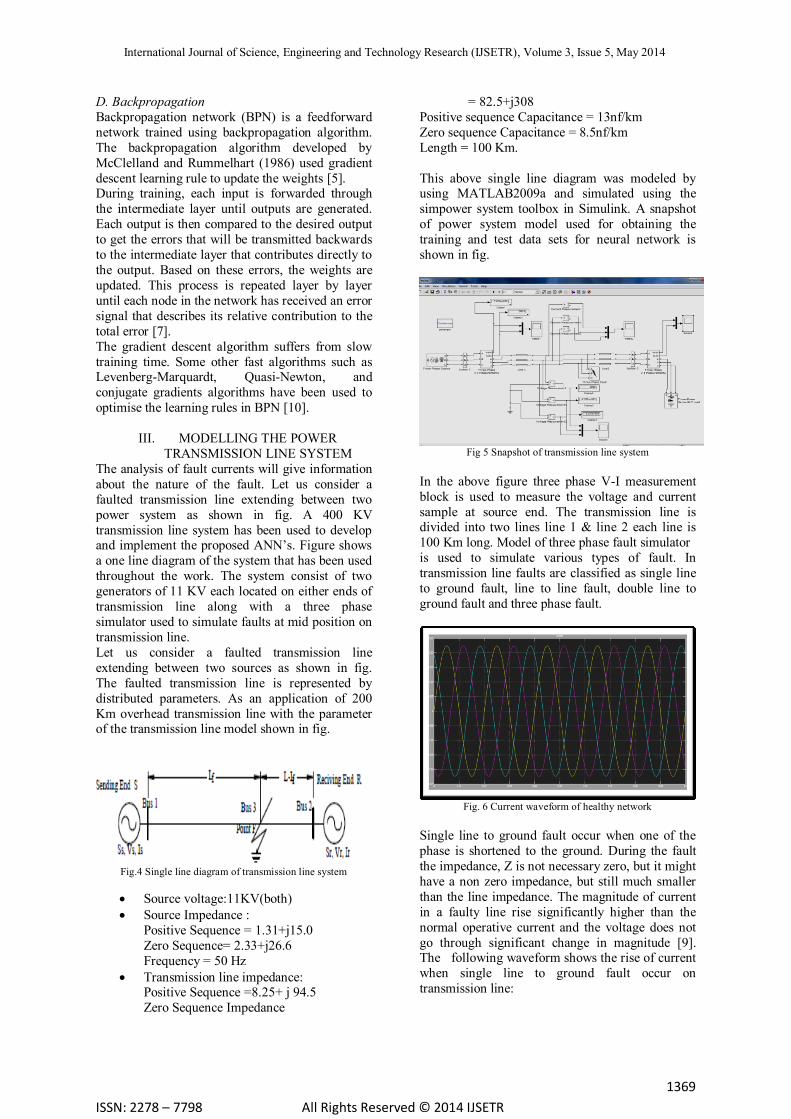
Fig 5 Snapshot of transmission line system

In the above figure three phase V-I measurement

block is used to measure the voltage and current

sample at source end. The transmission line is divided into two lines line 1 & line 2 each line is

100 Km long. Model of three phase fault simulator

is used to simulate various types of fault. In

transmission line faults are classified as single line

to ground fault, line to line fault, double line to

ground fault and three phase fault.

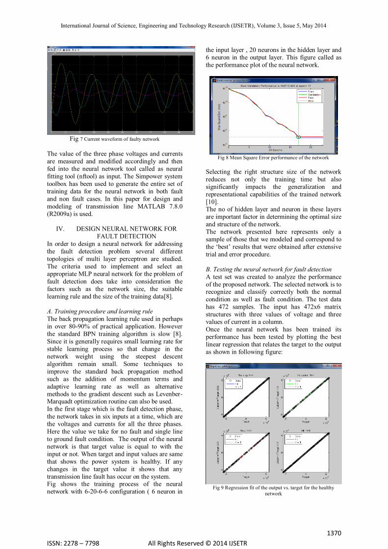
Fig. 6 Current waveform of healthy network

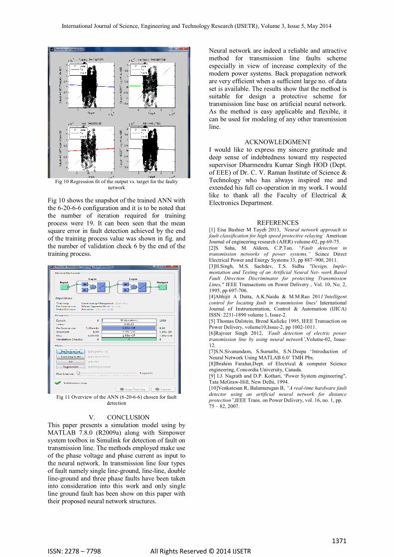
Single line to ground fault occur when one of the

phase is shortened to the ground. During the fault

the impedance, Z is not necessary zero, but it might

have a non zero impedance, but still much smaller

than the line impedance. The magnitude of current

in a faulty line rise significantly higher than the

normal operative current and the voltage does not

go through significant change in magnitude [9]. The following waveform shows the rise of current

when single line to ground fault occur on

transmission line:


1370


Fig 7 Current waveform of faulty network

The value of the three phase voltages and currents

are measured and modified accordingly and then

fed into the neural network tool called as neural

fitting tool (nftool) as input. The Simpower system

toolbox has been used to generate the entire set of

training data for the neural network in both fault

and non fault cases. In this paper for design and

modeling of transmission line MATLAB 7.8.0

(R2009a) is used.

IV. DESIGN NEURAL NETWORK FOR

FAULT DETECTION

In order to design a neural network for addressing

the fault detection problem several different

topologies of multi layer perceptron are studied.

The criteria used to implement and select an

appropriate MLP neural network for the problem of

fault detection does take into consideration the

factors such as the network size, the suitable

learning rule and the size of the training data[8].

A. Training procedure and learning rule

The back propagation learning rule used in perhaps

in over 80-90% of practical application. However

the standard BPN training algorithm is slow [8].

Since it is generally requires small learning rate for

stable learning process so that change in the

network weight using the steepest descent

algorithm remain small. Some techniques to

improve the standard back propagation method

such as the addition of momentum terms and

adaptive learning rate as well as alternative

methods to the gradient descent such as Levenber-Marquadt optimization routine can also be used.

In the first stage which is the fault detection phase,

the network takes in six inputs at a time, which are

the voltages and currents for all the three phases.

Here the value we take for no fault and single line

to ground fault condition. The output of the neural

network is that target value is equal to with the

input or not. When target and input values are same

that shows the power system is healthy. If any

changes in the target value it shows that any

transmission line fault has occur on the system. Fig shows the training process of the neural

network with 6-20-6-6 configuration ( 6 neuron in

the input layer , 20 neurons in the hidden layer and

6 neuron in the output layer. This figure called as

the performance plot of the neural network.

Fig 8 Mean Square Error performance of the network

Selecting the right structure size of the network

reduces not only the training time but also

significantly impacts the generalization and

representational capabilities of the trained network

[10]. The no of hidden layer and neuron in these layers

are important factor in determining the optimal size

and structure of the network.

The network presented here represents only a

sample of those that we modeled and correspond to

the ‘best’ results that were obtained after extensive

trial and error procedure.

B. Testing the neural network for fault detection

A test set was created to analyze the performance

of the proposed network. The selected network is to recognize and classify correctly both the normal

condition as well as fault condition. The test data

has 472 samples. The input has 472x6 matrix

structures with three values of voltage and three

values of current in a column.

Once the neural network has been trained its

performance has been tested by plotting the best

linear regression that relates the target to the output

as shown in following figure:

Fig 9 Regression fit of the output vs. target for the healthy

network


1371


Fig 10 Regression fit of the output vs. target for the faulty

network

Fig 10 shows the snapshot of the trained ANN with

the 6-20-6-6 configuration and it is to be noted that

the number of iteration required for training

process were 19. It can been seen that the mean

square error in fault detection achieved by the end

of the training process value was shown in fig. and

the number of validation check 6 by the end of the

training process.

Fig 11 Overview of the ANN (6-20-6-6) chosen for fault

detection

V. CONCLUSION

This paper presents a simulation model using by

MATLAB 7.8.0 (R2009a) along with Simpower

system toolbox in Simulink for detection of fault on

transmission line. The methods employed make use

of the phase voltage and phase current as input to

the neural network. In transmission line four types

of fault namely single line-ground, line-line, double

line-ground and three phase faults have been taken into consideration into this work and only single

line ground fault has been show on this paper with

their proposed neural network structures.

Neural network are indeed a reliable and attractive

method for transmission line faults scheme

especially in view of increase complexity of the

modern power systems. Back propagation network

are very efficient when a sufficient large no. of data

set is available. The results show that the method is suitable for design a protective scheme for

transmission line base on artificial neural network.

As the method is easy applicable and flexible, it

can be used for modeling of any other transmission

line.

ACKNOWLEDGMENT

I would like to express my sincere gratitude and

deep sense of indebtedness toward my respected

supervisor Dharmendra Kumar Singh HOD (Dept.

of EEE) of Dr. C. V. Raman Institute of Science &

Technology who has always inspired me and extended his full co-operation in my work. I would

like to thank all the Faculty of Electrical &

Electronics Department.

REFERENCES [1] Eisa Bashier M Tayeb 2013, ’Neural network approach to

fault classification for high speed protective relaying’ American

Journal of engineering research (AJER) volume-02, pp 69-75.

[2]S. Saha, M. Aldeen, C.P.Tan, “Fault detection in

transmission networks of power systems,” Scince Direct

Electrical Power and Energy Systems 33, pp 887–900, 2011.

[3]H.Singh, M.S. Sachdev, T.S. Sidhu "Design, Imple-

mentation and Testing of an Artificial Neural Net- work Based

Fault Direction Discriminator for protecting Transmission

Lines," IEEE Transactions on Power Delivery , Vol. 10, No. 2,

1995, pp 697-706.

[4]Abhijit A Dutta, A.K.Naidu & M.M.Rao 2011’Intelligent

control for locating fault in transmission lines' International

Journal of Instrumentation, Control & Automation (IJICA)

ISSN: 2231-1890 volume 1, Issue-2.

[5] Thomas Dalstein, Brend Kulicke 1995, IEEE Transaction on

Power Delivery, volume10,Issue-2, pp 1002-1011.

[6]Rajveer Singh 2012, ’Fault detection of electric power

transmission line by using neural network’,Volume-02, Issue-

12.

[7]S.N.Sivanandam, S.Sumathi, S.N.Deepa ‘Introduction of

Neural Network Using MATLAB 6.0’ TMH Pbs.

[8]Ibrahim Farahat,Dept. of Electrical & computer Science

engineering, Concordia University, Canada.

[9] I.J. Nagrath and D.P. Kothari, ‘Power System engineering",

Tata McGraw-Hill, New Delhi, 1994.

[10]Venkatesan R, Balamurugan B, “A real-time hardware fault

detector using an artificial neural network for distance

protection”,IEEE Trans. on Power Delivery, vol. 16, no. 1, pp.

75 – 82, 2007.

simulation of fault detection for...

Documents