simulation of chemical enrichment in...
TRANSCRIPT

Simulation of Chemical Enrichmentin Galaxies
Master Thesisat the
Ludwig-Maximilians-Universitat Munchen
submitted by
Emilio Mevius
supervised by
Dr. Klaus Dolag
Munich, November 2016


Simulation Chemischer Bereicherungin Galaxien
Masterarbeitan der
Ludwig-Maximilians-Universitat Munchen
vorgelegt von
Emilio Mevius
betruet von
Dr. Klaus Dolag
Munchen, November 2016


Abstract
Galaxy formation models distinguish two main modes, how the stellar disc component of spiralgalaxies can grow. The disk grows either through formation of stars from newly accreted, mainlypristine material in the outer parts, or by consuming more enriched gas in the disk and grow fromthe inside out. Indication on which of the processes is dominant can be obtained by observations,especially from the correlation of different galactic properties. Observed radial profiles of thechemical enrichment-level currently support more the inside out model and give additional infor-mation of the evolution history. Star formation, gas in- and out-flows are fundamental processesin the evolution of galaxies, and the chemical enrichment, their ashes. The observed chemicalenrichment therefore is a key element for understanding galaxy formation and evolution. Thecorrelation between the stellar mass and the chemical content of galaxies is known already formany years and its slope, although not completely understood yet, is probably established by theaction of galactic winds, a key player for re-distributing mass and energy from the galactic feed-back processes. The mass-metallicity relation (MZR) therefore can be used to constrain differentfeedback models in numerical simulations. Still, the treatment of detailed chemical enrichmentin galaxies within cosmological simulations is a relative new field and many simulations fail toproperly reproduce the observed trends and evolution of the chemical enrichment in galaxies. Themain goal of this work is to make an up to date comparison of the MZR and the metallicity gra-dients seen in the latest observational data with the galaxies in the MAGNETICUM simulation,which follow a detailed model of stellar evolution and chemical enrichment, described in Tornatoreet. all 2007. This allows us to study the outcome of the simulations and to infer the influence ofdifferent feedback models, together with the effects of different numerical resolutions. In additionwe compare the influence of using different observational tracer for the metallicity by mimickingthe same selection criteria than observations, addressing the possible influence of numerical andobservational effects in discrepancies with observed trends, which will help to interpret currentand future results in this relatively new field.

Contents
Contents
List of Figures . . . . . . . . . . . . . . . . . . . . . . . . . . . . . . . . . . . . . . IList of Tables . . . . . . . . . . . . . . . . . . . . . . . . . . . . . . . . . . . . . . III
1 Introduction 11.1 Evolution of Stars . . . . . . . . . . . . . . . . . . . . . . . . . . . . . . . . . 1
1.1.1 Supernovae . . . . . . . . . . . . . . . . . . . . . . . . . . . . . . . . . 41.1.2 Compact Objects . . . . . . . . . . . . . . . . . . . . . . . . . . . . . 5
1.2 Evolution of Galaxies . . . . . . . . . . . . . . . . . . . . . . . . . . . . . . . . 61.2.1 Inside-Out Model . . . . . . . . . . . . . . . . . . . . . . . . . . . . . 61.2.2 Transition from Spiral- to Elliptical-Galaxies . . . . . . . . . . . . . . . 6
2 Mass-Metallicity Relation 82.1 Gas-Phase Metallicity . . . . . . . . . . . . . . . . . . . . . . . . . . . . . . . 82.2 Stellar Metallicity . . . . . . . . . . . . . . . . . . . . . . . . . . . . . . . . . 92.3 Evolution . . . . . . . . . . . . . . . . . . . . . . . . . . . . . . . . . . . . . . 9
3 Metallicity Gradients 103.1 Gradient in Galaxies . . . . . . . . . . . . . . . . . . . . . . . . . . . . . . . . 10
3.1.1 Gas-Phase Gradients . . . . . . . . . . . . . . . . . . . . . . . . . . . . 103.1.2 Stellar Gradients in Spiral Galaxies . . . . . . . . . . . . . . . . . . . . 113.1.3 Stellar Gradients in Elliptical Galaxies . . . . . . . . . . . . . . . . . . . 12
3.2 Gradients in Clusters of Galaxies . . . . . . . . . . . . . . . . . . . . . . . . . . 13
4 Observational Methods 164.1 Gas Mass . . . . . . . . . . . . . . . . . . . . . . . . . . . . . . . . . . . . . . 164.2 Stellar Mass . . . . . . . . . . . . . . . . . . . . . . . . . . . . . . . . . . . . 164.3 Metallicity . . . . . . . . . . . . . . . . . . . . . . . . . . . . . . . . . . . . . 17
4.3.1 Direct Method . . . . . . . . . . . . . . . . . . . . . . . . . . . . . . . 184.3.2 Strong-Line Analysis . . . . . . . . . . . . . . . . . . . . . . . . . . . . 194.3.3 Young Stellar Metallicity Method . . . . . . . . . . . . . . . . . . . . . 21
4.4 Galactocentric Distances . . . . . . . . . . . . . . . . . . . . . . . . . . . . . . 22
5 Simulating Chemical Enrichment 235.1 Star Formation . . . . . . . . . . . . . . . . . . . . . . . . . . . . . . . . . . . 235.2 Initial Mass Function . . . . . . . . . . . . . . . . . . . . . . . . . . . . . . . . 245.3 Lifetime Function . . . . . . . . . . . . . . . . . . . . . . . . . . . . . . . . . 275.4 Stellar Yields . . . . . . . . . . . . . . . . . . . . . . . . . . . . . . . . . . . . 275.5 Enrichment . . . . . . . . . . . . . . . . . . . . . . . . . . . . . . . . . . . . . 285.6 Distribution . . . . . . . . . . . . . . . . . . . . . . . . . . . . . . . . . . . . 30
6 Chemical Enrichment of Galaxies in MAGNETICUM 326.1 MAGNETICUM . . . . . . . . . . . . . . . . . . . . . . . . . . . . . . . . . . 32

Contents
6.2 Star Formation Efficiency . . . . . . . . . . . . . . . . . . . . . . . . . . . . . 346.3 Stellar Mass . . . . . . . . . . . . . . . . . . . . . . . . . . . . . . . . . . . . 346.4 Gas-Phase Metallicity . . . . . . . . . . . . . . . . . . . . . . . . . . . . . . . 36
6.4.1 Evolution . . . . . . . . . . . . . . . . . . . . . . . . . . . . . . . . . . 396.5 Stellar Metallicity . . . . . . . . . . . . . . . . . . . . . . . . . . . . . . . . . 396.6 Gas-Phase Gradients . . . . . . . . . . . . . . . . . . . . . . . . . . . . . . . . 416.7 Stellar Gradients . . . . . . . . . . . . . . . . . . . . . . . . . . . . . . . . . . 456.8 behavior of Further Elements in Stars . . . . . . . . . . . . . . . . . . . . . . . 49
7 Discussion 51
References 54
Affirmation 58
I List of Figures
List of Figures
1.1 Hertzsprung-Russell diagram . . . . . . . . . . . . . . . . . . . . . . . . . . . . 21.2 Chemical enrichment according to supernova type . . . . . . . . . . . . . . . . 51.3 Stellar metallicity of star forming- and quenching-galaxies . . . . . . . . . . . . 71.4 Transition from star forming- to quenching-galaxy . . . . . . . . . . . . . . . . 7
3.1 Gas-phase metallicity gradient of galaxies . . . . . . . . . . . . . . . . . . . . . 113.2 Stellar metallicity gradients in spiral galaxies . . . . . . . . . . . . . . . . . . . 123.3 Stellar metallicity gradients in elliptical galaxies . . . . . . . . . . . . . . . . . . 133.4 Metallicity gradients in galaxy clusters . . . . . . . . . . . . . . . . . . . . . . . 143.5 Metallicity gradients in the intracluster medium . . . . . . . . . . . . . . . . . . 15
4.1 Evolution of star formation efficiency . . . . . . . . . . . . . . . . . . . . . . . 174.2 Gas-phase metallicity with the extended direct method . . . . . . . . . . . . . . 194.3 Comparison of strong-line calibrations . . . . . . . . . . . . . . . . . . . . . . . 204.4 Young stellar metallicity method . . . . . . . . . . . . . . . . . . . . . . . . . . 21
5.1 Comparison of IMFs . . . . . . . . . . . . . . . . . . . . . . . . . . . . . . . . 255.2 Metal distribution according the IMF choice . . . . . . . . . . . . . . . . . . . 265.3 Comparison of lifetime functions . . . . . . . . . . . . . . . . . . . . . . . . . . 275.4 Comparison between sets of stellar yields . . . . . . . . . . . . . . . . . . . . . 285.5 Metallicity distribution according the wind model . . . . . . . . . . . . . . . . . 31
6.1 Evolution of the star formation efficiency in MAGNETICUM . . . . . . . . . . . 356.2 Comparison of galactic stellar mass with postprocessing estimation . . . . . . . 366.3 Gas-phase metallicity in MAGNETICUM . . . . . . . . . . . . . . . . . . . . . 386.4 Evolution of gas-phase metallicity in MAGNETICUM . . . . . . . . . . . . . . . 406.5 Stellar metallicity in MAGNETICUM . . . . . . . . . . . . . . . . . . . . . . . 426.6 Gas-phase metallicity gradient with space resolution constraints . . . . . . . . . 436.7 Gas-phase metallicity gradient . . . . . . . . . . . . . . . . . . . . . . . . . . . 446.8 Gas-phase metallicity gradient with temperature and composition constraints . . 456.9 Stellar metallicity gradient with space resolution constraints . . . . . . . . . . . 466.10 Dispersion in stellar metallicity gradients . . . . . . . . . . . . . . . . . . . . . 476.11 Stellar metallicity gradients from individual galaxies . . . . . . . . . . . . . . . . 486.12 Relations between element ratio abundances . . . . . . . . . . . . . . . . . . . 50


III List of Tables
List of Tables
6.1 Cosmological parameters used in MAGNETICUM . . . . . . . . . . . . . . . . . 326.2 Properties of the used resolutions in this work . . . . . . . . . . . . . . . . . . 326.3 Selection of simulations used in this work . . . . . . . . . . . . . . . . . . . . . 33

1 CHAPTER 1. INTRODUCTION
1 Introduction
1.1 Evolution of Stars
The Hertzsprung-Russell diagram (HRD) represents a universal distribution of stars in atemperature-luminosity matrix. The patterns found in the HRD reveal the paths followed bystars during their evolution. These paths through the HRD depend strongly on the initial mass.Differentiating by initial mass is therefore the best way to portray the different possible stellarevolutions.
The main sequence (MS) is the most obvious trend in the HRD, a nearly diagonal line goingfrom the faint red region to the bright blue one and is the place where live the most of the stars.The left panel in Figure 1.1 shows a typical picture of the HRD, where the main sequence crossthrough it, together with other recognizable regions.
The Hayashi line is a nearly vertical line on the right side of the HRD that marks the threshold ofhydrostatic equilibrium. The position of the line depends on the initial mass. The more massivethe stars are, the higher the needed temperature is, to reach the hydrostatic equilibrium. Thecollapse of the molecular cloud during the birth of a star finish by reaching the Hayashi line.After that, the surface brightness sink with nearly constant temperature until the hydrostaticequilibrium is reached.
The Henyey line appears for massive enough protostars (& 0.5 M) and represent the way fromthe Hayashi line to the main sequence. The temperature increase and the luminosity also, slightly.Through the nuclear fusion sink the luminosity again just before to enter the MS. The right panelin Figure 1.1 is portrayed the possible ways of a protostar according to its initial mass.
Having this tool is easier to follow the birth and evolution of stars. Star formation (SF) starts bythe gravitational collapse of a molecular cloud, mostly composed by H and He. Magnetic fieldsand turbulences could affect the stability of the molecular cloud during SF, but their role is stillpoorly understood. Otherwise, only the pressure out of the hydrostatic conditions acts againstthe gravitation. The Jeans criterion gives a threshold mass, called Jean’s mass MJ , for which thethermic energy cannot counteract the gravitation energy any longer and avoid the gravitationalcollapse. Under the assumptions of spherical symmetry and constant density, the MJ reaches:
MJ =
(5kT
Gm
)3/2(3
4πρ
)1/2
(1.1)
Where k is the Boltzmann constant, T is the temperature, G is the gravitation constant, m isthe mass per particle in the cloud and ρ is an assumed constant density. Any molecular cloudwith a mass bigger than MJ , should theoretically collapse.
By all matter with a temperature greater than the absolute zero, interatomic collisions cause the

1.1. EVOLUTION OF STARS 2
Figure 1.1: Left: Hertzsprung-Russell diagram showing the position of some known stars. Credits: ESO. Right:
Pre-main-sequence evolutionary paths (PMS), i.e. the way to get to the main sequence (MS). The black line
placed top right run through the birth places of stars of different masses. The blue lines represent the PMS and
the black line placed at the bottom left represents the MS. The end of the path is addressed with the stellar mass
in solar units. The nearly vertical blue lines are known as the Hayashi lines, while the nearly horizontal ones as the
Henyey lines. As seen in the graphic, taken from Steven and Palla (2008), the most massive stars born directly
on the Henyey line and stay there until they reach the MS. Average stars go through the Hayashi line before to
turn to the Henyey line. The lightest ones instead, stay on the Hayashi Line until they reach the MS. The red
lines represent Isochrones, i.e. lines that connect the points of constant age through the different paths.
kinetic energy of the atoms to change and set electromagnetic radiation free. This emission iscalled thermal radiation. The first thermal radiations coming from the conversion of gravitationalenergy into thermic energy in the core are emitted until the density in the surface increase enoughto be optical thick. Before that, just radiative losses are present, i.e. the flux from regions withoptical thin layers.
After the outer shells become optical thick, the thermic energy can oppose the gravitationalenergy and subsequently stops the first collapse. The radius of the first hydrostatic core (FHSC),also called pre-stellar core, reaches 10 to 20 AE for average stars. This free fall phase takes ∼10000 years until the temperature in the core is big enough to split the H2 molecules in single Hatoms.
The consumed energy for transforming molecular H in atomic H is not used any longer for thestability of the core, starting a second big collapse. A new hydrostatic equilibrium is reached ofthe same way and the core of the now called protostar reaches only ∼ 1.5 R in average.
From here on, the protostar is victim of the continuous incursion of mass from the surroundingsand gains mass. This phase, called main accretion phase, is the key stage to decide if the protostarbecomes a star. As star are recognized only the objects, which in this phase reach a temperaturehigh enough to start the nuclear fusion of the H atoms. The fusion of H starts by ∼ 3·109 K andthis is only possible with an initial stellar mass from ∼ 0.07 M up. Here start the true life of

3 CHAPTER 1. INTRODUCTION
the stars, if starts. The different life paths depend from here on, on the initial mass.
• Until ∼ 0.3 M are considered mass poor stars. They stay in the Hayashi line until toreach the MS, as showed in Figure 1.1. The temperature in this case was just enough tostart the H fusion, and this keep going the slowest. Red dwarfs can live over 1012 years.Almost 2/3 of all stars are red dwarfs. After finally staying without fuel, they contract andreach a diameter of some thousands of km. At this stage the stabilization is only possiblethrough the degenerated pressure of the electrons. The properties of degenerated matterappears hereby when the density is big enough or the temperature low enough, so that thebehavior deviates of the classic physics, giving space to quantum physical effects.
• From ∼ 0.3 M until ∼ 2.3 M are considered sun-like stars. They live around ∼ 109
years. These stars are massive enough to reach enough temperature in the core to startthe fusion of He, one of the products of the previous H fusion. All processes overlap, sothe He-phase starts when there is still some H in the core and in the shell. Stars are builtwith shell after shell with the heavier elements going inside out. The He fusion produceenough temperature to fusion the H in the shell and make the star expand. With theexpansion of the star and growth of its luminosity, the stars follow a diagonal path in theHRD known as the red giant branch (RGB). There are many branches and subbranchesand we review only the most outstanding ones. After the so called He-flash, a big energyrelease raise the temperature of the core at the point that is not degenerated any more.The lower pressure lets the size of the star sink, maintaining the luminosity nearly constant.This produce a nearly horizontal path in the HRD, the horizontal branch (HB). When theHe in the core is over, the temperature in the core decrease and the star contracts. Thecontraction, nevertheless, produce enough temperature for He fusion in the shell, makingthe star expand and its luminosity grow. This diagonal path is the second most notablepath in the HRD after the MS and is known as the asymptotic giant branch (AGB), wherered giant stars are placed in the left panel in Figure 1.1. At this point there is H and Healmost exclusively in the shell and a burning core of C and O. During this trip is common tolose high amounts of mass from the shell through stellar winds, also called AGB-winds, dueto the impossibility to keep maintaining these layers gravitational coupled. Momentum-driven-winds are called the stellar winds that carry the momentum of the radiation pressurefrom continuous absorption and scattering from the stellar activity and nearby SNe. Onlythe most massive stars form also a so called planetary nebula around them. When the fuelof He is finally over, these stars contract and end up as white dwarfs (WD).
• From ∼ 2.3 M until ∼ 3 M, stars are already able to start the fusion of C. In thismass range is so much mass lost through the AGB-winds, that the Chandrasekhar limitis not reached and they end up as WD as well. This limit (∼ 1.4 M) is the maximumpossible mass for a stable WD. As soon as this threshold is reached, the core collapses inmatter of seconds and the shell is spread violently away through the energy that is set freemostly in form of neutrinos. This is a so called supernova (SN) explosion. Further detailsabout SN types are given in Section 1.1.1.
• Over ∼ 3 M is considered the range of the most massive stars. They can consume theirwhole fuel in just some hundred thousand years. They hike to the region of super giantsthrough their own super giant branch after their short stay in the MS, as can be seen inthe left panel in Figure 1.1. The biggest part of the star gather together in a Fe core of ∼10000 km of diameter until the SN explosion. The core of exploding super massive stars

1.1. EVOLUTION OF STARS 4
is only stabilized through a degenerated pressure, in this case of neutrons. This remains,together with WDs, are called compact objects, further described in Section 1.1.2.
Is remarkable, that the metals (in Astronomy heavier elements than He) could also play a roleduring the life of the stars, affecting the duration of the fusion phases as well as the formationof magnetic fields and how strong become the stellar winds. Evolutionary processes related tometallicity in astronomy are in general poorly understood and represent a new field.
1.1.1 Supernovae
Understanding the role of supernovae (SN) is a key step to reproduce the observed chemicalenrichment in galaxies. SN explosions represent the principal mechanism to enrich the environ-ment with heavy metals. Together with the stellar winds, define the enrichment, as well as thedistribution of the elements by means of the transferred momentum.
The most representative types of SN are the SNIa and SNII
• SNIa: Arises from a binary system with mass in the range 0.8-8 M. Under this variant,a white dwarf (WD) trap another star in his gravitational field and accretes gradual itsmass until to reach near exactly the Chandrasekhar limit. Because of the closeness to thetheoretical limit where a SN explosion is possible, these events are presumed to have nearlythe same mass, expelled energy and luminosity, becoming commonly used standard candlesto measure distances in the deep space. After the explosion stays no compact object behindand the partner star is hurled away.
• SNII: Arises with masses of m & 8 M. The typical feature to recognize this kind of SNis the appearance of spectral lines of H. This explosion is a natural part in the life of starswith masses above 3 M. They don’t need extra accretion of mass from some neighbourstar to reach the Chandrasekhar limit.
The contribution of each SN can be understood through the different fusion processes that takeplace during the life of a star ending up as one type of SN or the other. The most importantreaction during the H-phase is called the triple-alpha process and produce mostly He that gathertogether in the core. To a lesser extent are synthesized by-products like Li and Be. During theHe-phase is synthesized mostly C through the by-product Be and elements until O. The next bigfusion process, the one of the C, synthesize O properly and further elements until Fe. Furtherfusion processes produce other elements to a lesser extent. Each fusion level release less energythan the previous one and run faster out. By Fe stops the fusion chain, since Fe has the highestbinding energy and the fusion to heavier elements consumes energy instead of release it. The halfof the elements beyond Fe is released to the ISM through the r-process, the nucleosynthesis thattakes place in the outer shells of the Fe core during a SNII explosion. The other half is releasedby stellar winds during the AGB-phase.
The stellar yields represent the mass ejected from a star into the ISM, consisting of preexistingmatter together with newly formed. Depending on the initial mass, the production of a certainamount of the different elements is expected according to the physical processes in stars of thismass. In Figure 1.2 is plotted the abundance number ratios to Fe in the cluster Abel 262. Thesevalues were fitted in Sato et al. (2009) by a combination of SNIa and SNII yields per supernova

5 CHAPTER 1. INTRODUCTION
to get the number of SNIa and the ratio SNII to SNIa. The SNIa yields were hereby betterrepresented by the SNIa model W7 over the models WDD1 and WDD2. The ratio SNII to SNIawas estimated as 3 to 1, that means, only one fourth of all SN were SNIa. This result is similarfor other clusters.
Figure 1.2: Abundance number ratio of elements to Fe for the cluster Abel 262 in solar units (Sato et al.,
2009). The top and the bottom panels show the fits for the abundances inside 0.27 r180 and 0.1 r180, respectively.
The red points show the values in the cluster, while the blue dashed and solid lines show the contribution of SNIa
and SNII, respectively. For more information see Sato et al. (2009)
One can infer from the fit in Figure 1.2 the contribution from each SN type to the observedabundance of each element as well. We can learn from these results, therefore, from whichevents the enrichment comes from. By looking at the distribution of the elements is possible totrace the events inside a cluster and its galaxies and gain a wider view about galaxy evolutionand cluster evolution. In section 3 are treated the different metallicity gradients in clusters ofgalaxies.
1.1.2 Compact Objects
There are three classified compact objects: white dwarfs (WD), neutron stars (NS) and blackholes (BH). The conditions under which a compact object becomes NS or BH remain unknown.They have following features, described briefly:
• Neutron star: They have extreme high densities of about 1011 to 2.5·1012 kg/cm3, thescale of atomic cores. They count with a diameter of only ∼ 20 km and mass in the rangeof 1.4-3 M.
• Black hole: These compact objects are predicted in the general relativity as massive enoughto deform spacetime. These objects exhibit such a big gravitational force that not even

1.2. EVOLUTION OF GALAXIES 6
photons can escape from their field. The threshold by which is not possible any more toescape is called the event horizon. Observationally appear as empty regions that produceenormous gravitational effects as gravitational lensing.
1.2 Evolution of Galaxies
1.2.1 Inside-Out Model
The disc of young galaxies grows, according to this model, from inside out through accretion ofgas. The accreted gas towards the center triggers star formation (SF) when it is dense enough.
In Pastorello et al. (2014) is explained a two phases model. A first phase along z > 2 is calleddissipative collapse. The SF at this stage is driven by the infall of cold gas or by cooling ofhot gas. A second phase is called external accretion, by which usually old star populations areaccreted. These propositions are in concordance with the observed negative metallicity gradients,usually steeper at large radii. Age and metallicity gradients show old metal rich stars in a metalrich environment in the inner region and young metal poor stars in a metal poor environment inthe outer region.
This model is also supported by color gradients, SF history and a mass-size relation almostindependent of the redshift. The proportionality between mass and radius depends just slightlyon the virialization redshift, because systems that virialized first have larger mean initial densities,since the Universe was denser then (Chiosi et al., 2012).
1.2.2 Transition from Spiral- to Elliptical-Galaxies
Two clear trends for the stellar mass-metallicity relation (MZR) are recognized, the one of typicalspiral, gas rich, star forming galaxies, and the one of typical elliptical, passive, quenching galaxies.In Figure 1.3 is shown the stellar MZR obtained from a big survey of all kind of galaxies, presentedin Gallazzi et al. (2005), together with a differentiated plot of spirals and elliptical presented inPeng et al. (2015) from the same survey used by Gallazzi et al. (2005).
The difference of the slopes throw more lights in the transition from star forming- to quenching-galaxies, which seems to be part of the evolutionary process of all galaxies. In Figure 1.4 isillustrated the two possibilities for the transitions, explained in Peng et al. (2015). The firstoption is a slow gas loss caused by gas removal, due to tidal forces by approaching the center ofa cluster. The second one is the so called galaxy strangulation, where galaxies keep forming starsuntil they run out of gas. This process is probably enhanced by starbursts produced in majormerger events. There is almost never a collision between stars during a major merger, but theHII regions are agitated and trigger SF more rapidly than the usual rate. This galaxies are calledthen starbusts galaxies.
Elliptical galaxies show mostly higher stellar metallicities out of the slope of typical spiral galaxies,as can be seen in Figure 1.3, which supports an accelerated SF activity and the second scenarioas the most common, or the most determinant, in the quenching process.

7 CHAPTER 1. INTRODUCTION
Figure 1.3: Left: Stellar mass-metallicity Relation (MZR) as observed (Gallazzi et al., 2005). The big scatter
is caused by the mixture of spiral and elliptical galaxies (star forming and quenching), which show different curves.
Right: The different stellar MZR curves where star forming- and quenching-galaxies belong (Peng et al., 2015).
As indicated in the graphic, in the top on red are placed the quenching passive galaxies and down on blue the star
forming galaxies. Even a galaxy at redshift 1.4, a single galaxy measurement presented in Lonoce et al. (2015),
which should be placed below the curve of Gallazzi et al. (2005) for being in a higher redshift, appears above,
since it is a big elliptical, as can be seen in the left panel.
Figure 1.4: Two models for the transition from star forming- to a quenching-galaxy, taken from Peng et al.
(2015). a: Star formation (SF) stops by suffering gas removal. b: Galaxies keep forming stars until they run out
of gas. This last SF activity is probably accelerated, evidenced in the higher stellar metallicities out of the slope
of typical star forming galaxies, as illustrated in the MZR on the left side.
8
2 Mass-Metallicity Relation
A strong correlation between the stellar mass and the metallicity, was first observed by Lequeuxet al. (1979) for nearby irregular galaxies. Since there, many studies show similar results for everykind of galaxies out to z ∼ 3.
The mass-metallicity relation (MZR) shows the balance between gas inflow, the related starformation (SF) and gas outflow. Galactic outflows are observed to carry mass and metals to theIGM and they are produced principally by the composition of all the stellar winds within a galaxyand scale therefore with the star formation rate (SFR), but also with a fraction of the supernova(SN) energy that powers the wind.
Galactic outflows, however, depend not only on the own stellar activity of the galaxy, since asexplained in more detail in Section 1.2.2, the gas can also be pulled off by tidal forces from acluster. The SF self can be enhanced through a starbust produced by a big merger. The MZRdoesn’t represents a trivial relation that can be inferred from the physics of the stellar activity ina closed box model, but the result of a complex interplay that describes galaxy evolution globally.
The velocity of the galactic outflows scale with the escape velocity of the galaxy and also a bitwith the dispersion velocity (Davee et al., 2006). The mass-size relation ensures that the mostmassive galaxies are also bigger in general and retain more metals due to the stronger escapevelocity and therefore less effective galactic wind. The galactic outflows seem of this way to beresponsible for the slope of the MZR. Nevertheless, the nature of the MZR is not completelyunderstood.
2.1 Gas-Phase Metallicity
Represents the metallicity of the ISM in gas-rich galaxies, namely in HII star forming (SF) regions,which are typically heated (around 104 K) and ionised by the big amounts of UV radiation fromthe SF activity. The O absorption lines are relative easy to observe from the spectrum of thesenebulae, so is the O abundance used as reference for the metallicity in the gas.
The following expression is commonly used to describe the gas-phase metallicity:
12 + log10
(O
H
)(2.1)
Where the ratio (O/H) represents the number ratio and not the mass ratio. This ratio, logarith-mic, gives a slope suitable to analyse and compare. Using the semianalytical simulation FIRE,Ma et al. (2016) gives a linear approximation of the gas-phase metallicity, where the dependenceon the redshift is included.

9 CHAPTER 2. MASS-METALLICITY RELATION
2.2 Stellar Metallicity
Represents the mean metallicity between all stars in the galaxy. While the gas-phase metallicityrepresents the actual highest metallicity level of the galaxy, the stellar metallicity represents amean value through the time.
Although in some works is used a composition of several element abundances, the most extendeddefinition for stellar metallicity is the following using the Fe content as reference, since for stellarspectra is convenient the observation of the Fe absorption lines:[
Fe
H
]= log10
(NFe
NH
)star
− log10
(NFe
NH
)sun
(2.2)
The correlation is stronger for galaxies between 109 M and 1012 M. For less massive galaxiesis shown a smaller and irregular star formation efficiency and so the chemical enrichment (Maet al., 2016). An example of the stellar MZR can be seen in Figure 1.3 in Section 1.2.2, whereis also shown the different behaviors for spiral- and elliptical-galaxies.
2.3 Evolution
Many independent works show an evolution in the MZR with redshift. Not surprising, a highermetallicity is observed by smaller redshift, showing how there is more metals produced with thepass of the time. Interesting is how the MZR seems to keep its shape, probing its universalmeaning. The shape of the MZR is established probably around z ∼ 6 and remains constantafter that, getting slowly just higher values, and flattening slightly its slope (Davee et al., 2006).
Stars synthesize metals through the internal nuclear fusion processes during their evolution andgalactic outflows are observed to carry these elements to the IGM (Davee et al., 2006). Theseobservations together with the insights acquired from gradients in clusters, explained in moredetail in Section 3, throw away the possibility of a closed box model for the chemical evolutionof galaxies. Some authors use the name leaky-box model because the apparently inevitable fateof the galaxies of finally losing their gas fuel.
Examples of the gas-phase MZR and its evolution can be seen in Section 4.3, where is describedthe related observational methods.

10
3 Metallicity Gradients
The distribution of the metals within a galaxy depends clearly on the mass of the galaxy. Forthe least massive Galaxies, around 106 M, the distribution is smooth, but dwarf lost almost allmetals in the CGM and IGM. around 109 M the most of the metals are already placed inside10% of the virial radius Rvir, while for the most massive ones, around 1012 M, almost all ofthem are inside. This behavior is well reproduced in simulations, as reported in Ma et al. (2016)and consistent with the fact, that by smaller galaxies the metals can be spread out over a longerradius due to the smaller escape velocity of the galaxy. Galaxies heavier than 106 M (Ma et al.,2016) instead, keep a big portion of the metals, since the galactic winds fail leaving the Galaxyand these metals are reaccreted.
3.1 Gradient in Galaxies
Early comparisons of metallicity gradients taking the absolute galactocentric distances showed anyagreement between each other. It was realized that a common distance related to the physicalproperties of the galaxies should be chosen. The effective radius Reff is shown to be a goodnormalization choice for the galactocentric distances.
3.1.1 Gas-Phase Gradients
In Figure 3.1 is evident the general decaying gradient for the O abundance. This tendency wasanalysed in Sanchez-Menguiano et al. (2016) to find dependencies with other galaxy propertieslike morphology, luminosity and the presence of bars. This slope seems to be independent on anyother galaxy property but on the mass.
The mass classification in Figure 3.1 shows how the values of the metallicity go up, the moremassive the galaxies are, as expected from the slope of the MZR, always maintaining the shapeof the profile nearly equal. The special behaviors in the inner and outer regions start also in thesame place in any case. Bigger than ∼ 2 Reff flatten out every of them, while lower than ∼ 0.5Reff go down the most massive ones.
Active galaxy nuclei (AGN) are galaxies with a supermassive black hole (BH) in the center. AGNactivity hinder the spectroscopy but also could push metals away from the center, if present. Theinner region of the most massive bins flatten despite of the effort made in Sanchez-Menguianoet al. (2016) for excluding strong AGNs as well as weak AGNs. The nature of the flattenings inboth, the inner and the outer region, remain a mystery.
Barred spiral galaxies are spiral galaxies with a central bar-shaped structure, usually called the

11 CHAPTER 3. METALLICITY GRADIENTS
Figure 3.1: Sanchez-Menguiano et al. (2016) present this radial profile of gas-phase metallicity gradient
averaged from 122 face-on spiral galaxies from the CALIFA survey. The symbols represent the mean value and
the bars the standard deviation. Four different mass bins were chosen in a way to ensure a comparable number
of galaxies in each bin. Blue diamonds: log(M/M) ≤ 10.2. Red squares: 10.2 < log(M/M) ≤ 10.5. Yellow
circles: 10.5 < log(M/M) ≤ 10.75. Purple triangles: 10.75 < log(M/M). The dashed vertical lines separate
the three different behaviors.
bars, that concentrate ISM gas and stars. 30% - 40% of spiral galaxies have strong bars in theoptical wavelength range and 60% if weak bars are considered (Sanchez-Menguiano et al., 2016).Some simulations predict that the presence of bars can produce this effect in the inner region dueto the asymmetry they represent. Nevertheless, it was found no hint of such correlation accordingto Sanchez-Menguiano et al. (2016).
Some correlations were found in the past, only because the distances in each galaxy were expressedin absolute values and plotted together. In the most cases the correlations disappear afternormalization to a representative distance. The Reff seems to be the best choice so far, since itcorrelates with many other galaxy properties (Sanchez-Menguiano et al., 2016). For all furthercomparison with the results of the MAGNETICUM simulations in this work is used the Reff tonormalize the radial profiles.
Because of the technical difficulty, there are no numerous observations of gas gradients at higherredshifts. However, with new observational techniques is possible to build metallicity gradientsuntil higher radii, about 8 Reff, and at higher redshifts, about z ∼ 2. At this redshifts some gasgradients are rather positive, indicating possibly cold accretion or mergers that happen at themoment, the latter being difficult to distinguish (La Barbera et al., 2012).
3.1.2 Stellar Gradients in Spiral Galaxies
There is lack of representation of one dimensional stellar metallicity gradients in spiral galaxiesfrom available observational data. A comparison with the results of the MAGNETICUM simula-tions for the analysis, can be done therefore only for stellar gradients in elliptical galaxies. Figure

3.1. GRADIENT IN GALAXIES 12
Figure 3.2: Two dimensional stellar metallicity gradient of the spiral galaxy NGC 7549 from the CALIFA survey,
luminosity-weighted on the left and mass-weighted on the right. Color coded is the stellar metallicity. Taken from
Sanchez-Blazquez et al. (2014).
3.2 shows a two dimensional gradient presented in Sanchez-Blazquez et al. (2014).
The flattening in the gas-phase metallicity seen in observations at higher radii is know to appearalso by stellar metallicity gradients, suggesting an universal behavior.
As suggested in Sanchez-Menguiano et al. (2016), assuming the inside-out model, the stellaractivity is not enough to produce the enrichment seen in the outskirts and it could be rathera consequence of minor mergers, disturbance of satellite galaxies or metal recycling. All thesefactors are not independent of each other and more information is needed to make a more accurateanalysis.
3.1.3 Stellar Gradients in Elliptical Galaxies
The gradients of elliptical galaxies usually look more flat than the ones of spiral galaxies. Thisshould reveal the origin of elliptical galaxies as the merger of two spiral galaxies, since from themerger follows the mixing of the content distribution. This scenario was confirmed several timesin simulations. The metals produced by the stellar activity are the ashes of the evolutionary pro-cesses, in particular the observation of the stellar metallicity gradient, is the only true unequivocalproof of a merger event, not even the morphology.
While in-situ star formation (SF) and energy dissipation are the main processes to grow in earlyphases, accretion through minor mergers is seen in the later phases as the main origin of growingin size and shaping the metallicity gradients in massive galaxies at large radii.
At later phases, the accretion of old populations of metal poor stars is achieved without toinfluence the inner region of the galaxy. So is increased the Reff and the Sersic index, which givesthe radial profile of the surface brightness in single galaxies. A higher index indicates a higherluminosity in the center and a faster decay with the galactocentric distance.
Until 4 - 5 Reff should be dominated by in-situ SF. From here on is still unclear if the stars wereaccreted or built in-situ, closer to the center, and then migrated to the outside. Insights aboutthe latter would be key to understand the meaning of the AGN feedback. Massive galaxies byabout 1013 M are thought to have 40% till 60% of its stellar mass obtained by accretion, whilesmaller ones, without a big major event triggering starbust, until 95% (La Barbera et al., 2012).

13 CHAPTER 3. METALLICITY GRADIENTS
After major mergers instead, the gradients flatten. In a major merger, two galaxies of comparablesize merge and the dark matter of the system mix into the center through violent relaxation, i.e.a redistribution of the kinetic energy to reach thermic balance. The abundances mix hereby evenat large radii (La Barbera et al., 2012).
Figure 3.3 shows mean gradients of elliptical galaxies separated in three mass regions. Despiteof the irregularity in the lowest mass bin, the gradients shown to have in general higher values,the higher the mass is, as expected from the MZR. The shape of the gradients shows to be alsoindependent of the mass and therefore universal.
Figure 3.3: Typical abundance radial profiles of stellar metallicity in elliptical galaxies, taken from La Barbera
et al. (2012). The galactocentric distance is expressed logarithmic with the effective radius Reff as unity.
3.2 Gradients in Clusters of Galaxies
Figure 3.4 shows the gradients of different elements in the cluster Hydra A. Galaxy clusterswith cold cores, like this one, show specially good spectral lines, as explained in more detail inSection 4.3. These gradients show, like in other clusters (lower panel in Figure 3.4), peaks ofthe elements in the center and a regular decaying behavior. Specially Fe shows a clear peak,suggesting a predominant SNIa enrichment in the central dominant galaxies, according to thedifferent supernova (SN) yields shwon in Section 1.1.1. Nevertheless, the metal production inthe central galaxies doesn’t enrich automatically the ICM. It was already shown that AGN-ICMinteraction play a determinant role in the transport of metals from the big central galaxies to theICM (Simionescu et al., 2009).
From these gradients we can learn more about cluster evolution. The number of SNIa needed toreproduce the observed peaks of Fe, as well as the magnitude of stellar winds, are not enough toreproduce the observed peak of O. This suggests that there was a stronger SNII activity in thecentral region of the cluster in early phases, instead of a well mixed activity, as it was thoughtearlier (Simionescu et al., 2009).

3.2. GRADIENTS IN CLUSTERS OF GALAXIES 14
Figure 3.4: Top: Abundance radial profiles of the four elements indicated in the graphic for the cluster of
galaxies Hydra A. Taken from Simionescu et al. (2009). The vertical dashed line, where the behavior clearly
changes, corresponds to the virial radius of the cluster. Middle and bottom: Comparison of the Fe and O profiles,
respectively, with the other galaxy clusters indicated in the graphic. The radius is normalized to the virial radius
of the cluster r200.
15 CHAPTER 3. METALLICITY GRADIENTS
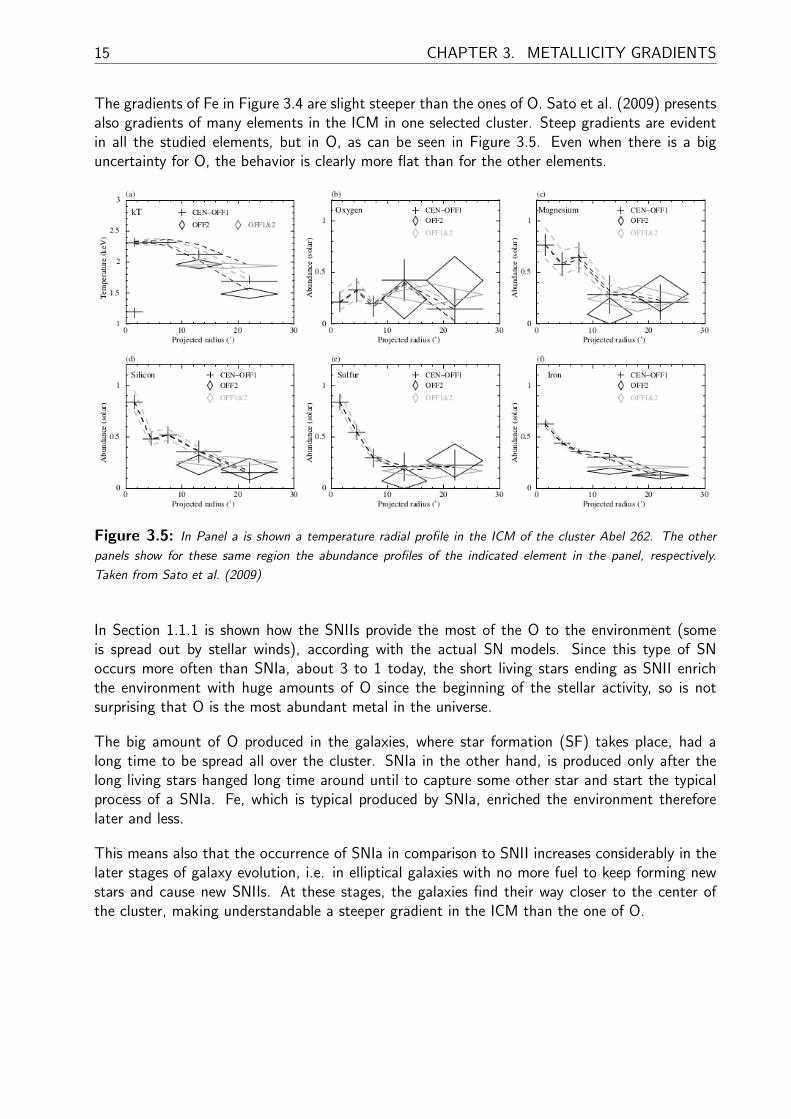
The gradients of Fe in Figure 3.4 are slight steeper than the ones of O. Sato et al. (2009) presentsalso gradients of many elements in the ICM in one selected cluster. Steep gradients are evidentin all the studied elements, but in O, as can be seen in Figure 3.5. Even when there is a biguncertainty for O, the behavior is clearly more flat than for the other elements.
Figure 3.5: In Panel a is shown a temperature radial profile in the ICM of the cluster Abel 262. The other
panels show for these same region the abundance profiles of the indicated element in the panel, respectively.
Taken from Sato et al. (2009)
In Section 1.1.1 is shown how the SNIIs provide the most of the O to the environment (someis spread out by stellar winds), according with the actual SN models. Since this type of SNoccurs more often than SNIa, about 3 to 1 today, the short living stars ending as SNII enrichthe environment with huge amounts of O since the beginning of the stellar activity, so is notsurprising that O is the most abundant metal in the universe.
The big amount of O produced in the galaxies, where star formation (SF) takes place, had along time to be spread all over the cluster. SNIa in the other hand, is produced only after thelong living stars hanged long time around until to capture some other star and start the typicalprocess of a SNIa. Fe, which is typical produced by SNIa, enriched the environment thereforelater and less.
This means also that the occurrence of SNIa in comparison to SNII increases considerably in thelater stages of galaxy evolution, i.e. in elliptical galaxies with no more fuel to keep forming newstars and cause new SNIIs. At these stages, the galaxies find their way closer to the center ofthe cluster, making understandable a steeper gradient in the ICM than the one of O.

16
4 Observational Methods
Integral field spectroscopy (IFS) is a relative new observation technique that combines the spec-trography with imaging techniques to reach a better space resolution for spectra. This technologyoffered in the last years analysis of wider HII regions, key regions for inferring metallicities. Thatis the case of the CALIFA survey, from which many of the observational data used in this workcome from.
Is not the intention of this work to give a detailed description of the observational methods, norto describe in detail the quantenmechanical concepts needed to follow some of them, but givinga view of the basics related to these, since the understanding of the conditions and limitationsof the observations help to improve a more reasonable comparison with the data obtained fromsimulations. In the following there is a brief description of the measurement of mass and metallicityof gas and stars.
4.1 Gas Mass
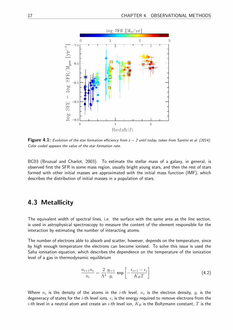
In Santini et al. (2014) is explained how the mass of the gas is usually obtained from spectralemission lines from the dust in warm regions, in a process that systematically underestimate thetotal mass by ∼ 50%. In that work is presented the evolution of the star formation efficiency(SFE), in Figure 4.1, which is expressed as the star formation rate (SFR) divided by the enclosedgas mass. In this work was probed that the best fit with these observations are only achievedwhen the estimated gas mass from the simulations is reduced to the half to get artificially thereported error in the observational data.
4.2 Stellar Mass
The mass of a star can only be directly estimated from a binary system of stars. This mass islater used as a sample to estimate indirectly the mass of other stars with the same properties inthe Hertzsprung-Russell diagram (HRD).
The mass-luminosity relation, showed below, is also a widely used tool to approximate the massof stars and even the stellar mass of a galaxy.
L
L≈=
M
M
3.5
(4.1)
More precise methods have been developed to estimate the galactic stellar mass, than roughlyusing the mass-luminosity relation. The most used recipe in the last years has been the method
17 CHAPTER 4. OBSERVATIONAL METHODS
Figure 4.1: Evolution of the star formation efficiency from z ∼ 2 until today, taken from Santini et al. (2014).
Color coded appears the value of the star formation rate.
BC03 (Bruzual and Charlot, 2003). To estimate the stellar mass of a galaxy, in general, isobserved first the SFR in some mass region, usually bright young stars, and then the rest of starsformed with other initial masses are approximated with the initial mass function (IMF), whichdescribes the distribution of initial masses in a population of stars.
4.3 Metallicity
The equivalent width of spectral lines, i.e. the surface with the same area as the line section,is used in astrophysical spectroscopy to measure the content of the element responsible for theinteraction by estimating the number of interacting atoms.
The number of electrons able to absorb and scatter, however, depends on the temperature, sinceby high enough temperature the electrons can become ionised. To solve this issue is used theSaha ionisation equation, which describes the dependence on the temperature of the ionizationlevel of a gas in thermodynamic equilibrium
ni+1neni
=2
Λ3
gi+1
giexp
[−εi+1 − εi
KBT
](4.2)
Where ni is the density of the atoms in the i-th level, ne is the electron density, gi is thedegeneracy of states for the i-th level ions, εi is the energy required to remove electrons from thei-th level in a neutral atom and create an i-th level ion, KB is the Boltzmann constant, T is the

4.3. METALLICITY 18
temperature of the gas and Λ the thermal de Broglie wavelength of an electron:
Λ =
√h2
2πmeKBT(4.3)
Where h is the Planck constant and me is the mass of an electron. AGN galaxies, however,are typical left from this analysis. For galaxies with AGN activity it is not feasible to infer thestar formation rate (SFR) and metallicity from the spectral lines as usual, since the AGN activityaffect the spectroscopy.
For the estimation of stellar metallicities are observed the absorption lines from the stellar at-mospheres, while for the estimation of gas-phase metallicities are observed the emission lines inHII regions of gas rich galaxies. These regions are typically heated (∼ 104 K) and ionised by theaction of the stellar activity and nearby supernovae.
Stellar metallicity measurements are more accurate and free of typical systematic errors observinggalactic nebulae. The limitation is the distance at which the spectroscopy for single stars can bedone. In general there is only available observations of stellar metallicity in the local universe.Lonoce et al. (2015) offers a estimation of the stellar metallicity of a single big elliptical galaxyat redshift 1.4.
The age of the stars can be estimated at the same time with stellar spectroscopy, among manyother methods. The Fe content in stars play a key role in this concern, since it is abundant andrelatively easy to observe, and a star without Fe was surely born in an early stage of the universe,where the environment was still not enriched with Fe. So is the Fe content commonly used asan indicator of the age of stars.
For the estimation of gas-phase metallicity in low mass galaxies is possible a direct measurementof the abundances in the ISM. For massive galaxies instead, is needed some calibration. Thesecalibrations use an empirical, theoretical or hybrid relation between observed ratios of strongemission lines in nebulae close to star forming regions, and the abundances of the elementsresponsible for the emissions. In the last years, however, a new method that infers the gas-phasemetallicity out of the metallicity of the youngest stars seems to overcome the problems of earliermeasurements, at least in the local universe, where stellar measurements are possible. All thesemethods are described in the following sections.
4.3.1 Direct Method
This is the only truly trustable method inferring metallicity from galactic nebulae. Spectroscopyof the temperature-sensitive [OIII] α 4363 line is used to infer the O content in nebulae directlyfrom the temperature of the electrons. This method is therefore also called the Te method. Theselines are specially weak in massive, metal-rich objects and their detection in individual galaxiesis in general only possible in the low mass end of the MZR, i.e. for galaxies in the stellar massrange of log(M/M) ∼ 7.4-8.9 (Andrews and Martini, 2013).
Andrews and Martini (2013) used stacked spectra of ∼ 200000 star-forming galaxies to enablethe detection of these temperature-sensitive lines in more massive galaxies and expand the direct

19 CHAPTER 4. OBSERVATIONAL METHODS
method to log(M/M) ∼ 10.5. In Figure 4.2 is shown a comparison of different strong-linecalibrations with the expanded direct method.
Figure 4.2: Circles and black line show the result of the direct method of gas-phase metallicity estimation
presented in Andrews and Martini (2013), for which the high mass limit is expanded from log(M/M) ∼ 8.9
to log(M/M) ∼ 10.5 by stacking the spectra of ∼ 200000 star-forming galaxies. In color is shown different
calibrations made with strong-line methods.
4.3.2 Strong-Line Analysis
The strongest spectral lines can be observed from the Earth and space until z ∼ 3. The mostaccurate methods to infer the metallicity in the gas, however, require the weak lines. Over z ∼0.2 is used exclusively strong-line methods. With these methods are observed the emission linesfrom warm ionised HII regions within star forming galaxies and the results are calibrated throughTe-based metallicities in the local universe.
These methods represent a process full of difficulties and systematic errors. In general is difficultto get absorption lines from warm gas, since from one specific temperature up, the atoms collideto each other in such a way that they become ionised and not longer suitable to absorb newenergy through their electrons (Simionescu et al., 2009).
Figure 4.3 shows a comparison of many different calibrations, each one apparently more appro-priate for mitigating problems related to observation conditions in different situations, like theobserved band, the absorption and even the redshift. The graphic shows a strong discrepancybetween one method and another in slope, absolute values and even the dispersion along themass range.
Knowing the discrepancies between calibrations, the comparison of gas-phase metallicities atdifferent redshifts may only be done between same calibrations. If no observation with a specificcalibration is available at some redshift, then is necessary to make a correction first. In Kewleyand Ellison (2008), Maiolino et al. (2008) and other works are given transformations betweencalibrations based on empirical relations. Only of this way is possible an analysis of evolution.

4.3. METALLICITY 20
Figure 4.3: In this graphic presented in Kewley and Ellison (2008) is perfectly seen the significant discrepancy
in values and slope for a bunch of the widely used strong-line calibrations for estimating the gas-phase metallicity.
In the upper frame is shown how even the scatter vary along the mass range in a different way for the different
calibrations.
Nevertheless, these procedure don’t erase the discouraging feeling, by looking at Figure 4.3,that probably none of these calibrations is close to the reality anyway. As Kewley and Ellison(2008) points out, the temperature fluctuations or gradients in th HII regions may cause wrongestimations of the electron temperature, from which is inferred the level of ionisation (see Equation4.2), key to estimate the chemical content.
Even using always the same calibration, there might be discrepancies at different redshifts. Thecomparison at different redshifts is just accurate if none of the involved physical properties evolvein time, like the gas density, ionisation, N/O ratio, among others, since they are assumed to beconstant by the calibration. Many of these properties are already probed to evolve. As pointedout in Maiolino et al. (2008), one of the main worries using these observational methods basedin strong emission lines, is that the dependence of these lines on metallicity involves also otherdependences and the evolution of these galaxy properties with redshift may easily affect thevalidity of the locally made calibrations, at higher redshifts. However, in Maiolino et al. (2008)is also presented a test that show how the deviation in the calibration between local galaxies andhigh redshift galaxies is only faint, about 0.1 dex. dex(x) represents one order of magnitude inlog10(x).
21 CHAPTER 4. OBSERVATIONAL METHODS
4.3.3 Young Stellar Metallicity Method
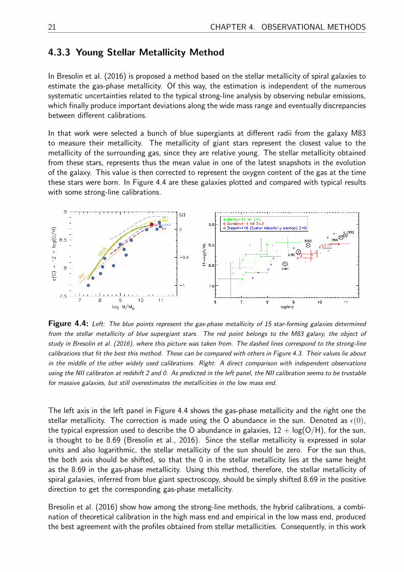
In Bresolin et al. (2016) is proposed a method based on the stellar metallicity of spiral galaxies toestimate the gas-phase metallicity. Of this way, the estimation is independent of the numeroussystematic uncertainties related to the typical strong-line analysis by observing nebular emissions,which finally produce important deviations along the wide mass range and eventually discrepanciesbetween different calibrations.
In that work were selected a bunch of blue supergiants at different radii from the galaxy M83to measure their metallicity. The metallicity of giant stars represent the closest value to themetallicity of the surrounding gas, since they are relative young. The stellar metallicity obtainedfrom these stars, represents thus the mean value in one of the latest snapshots in the evolutionof the galaxy. This value is then corrected to represent the oxygen content of the gas at the timethese stars were born. In Figure 4.4 are these galaxies plotted and compared with typical resultswith some strong-line calibrations.
Figure 4.4: Left: The blue points represent the gas-phase metallicity of 15 star-forming galaxies determined
from the stellar metallicity of blue supergiant stars. The red point belongs to the M83 galaxy, the object of
study in Bresolin et al. (2016), where this picture was taken from. The dashed lines correspond to the strong-line
calibrations that fit the best this method. These can be compared with others in Figure 4.3. Their values lie about
in the middle of the other widely used calibrations. Right: A direct comparison with independent observations
using the NII calibraton at redshift 2 and 0. As predicted in the left panel, the NII calibration seems to be trustable
for massive galaxies, but still overestimates the metallicities in the low mass end.
The left axis in the left panel in Figure 4.4 shows the gas-phase metallicity and the right one thestellar metallicity. The correction is made using the O abundance in the sun. Denoted as ε(0),the typical expression used to describe the O abundance in galaxies, 12 + log(O/H), for the sun,is thought to be 8.69 (Bresolin et al., 2016). Since the stellar metallicity is expressed in solarunits and also logarithmic, the stellar metallicity of the sun should be zero. For the sun thus,the both axis should be shifted, so that the 0 in the stellar metallicity lies at the same heightas the 8.69 in the gas-phase metallicity. Using this method, therefore, the stellar metallicity ofspiral galaxies, inferred from blue giant spectroscopy, should be simply shifted 8.69 in the positivedirection to get the corresponding gas-phase metallicity.
Bresolin et al. (2016) show how among the strong-line methods, the hybrid calibrations, a combi-nation of theoretical calibration in the high mass end and empirical in the low mass end, producedthe best agreement with the profiles obtained from stellar metallicities. Consequently, in this work
4.4. GALACTOCENTRIC DISTANCES 22
are preferred the comparisons with observations of metallicity estimated with these methods inthe last years.
The hybrid methods, namely the NII and O3N2 calibrations in Figure 4.3, corresponds to thefollowing strong-line ratios:
• NII: [NII]Hα
• O3N2: [OIII]α5007Hβ
· Hα[NII]α6584
For making these calibration is used the measurement of extragalactic HII regions, where it is ableto measure the abundance directly, and additionally the measurement of nebulae where the Oabundance can be inferred from photoionisation models that relate this ratio with the abundance.Then the model is fitted with the empirical data at high metallicities (Bresolin et al., 2016). Thesemethods are described in detail in Denicolo et al. (2002) (D02) and Pettini and Pagel (2004)(PP04), respectively.
4.4 Galactocentric Distances
Where is the end of a galaxy is not an easy question, since the mass of the galaxies spreadover a big and diffuse range. A widely used concept in astronomy to define a representativegalactocentric distance is the virial radius Rvir, within which virial equilibrium holds, that is, thevirial theorem in equation 4.4, holds. T represent the total kinetic energy of the system and Vthe total potential energy. The brackets represent an average over time.
2 < T >= − < V > (4.4)
At this radius the surrounding mass is considered bounded enough to the system. The massinside this radius is called therefore virial mass Mvir.
Observationally, is difficult to determine Rvir. In cosmology is often used an approximation asthe radius, within the mean density is greater than the critical density, in equation 4.5, by somefactor. Here is H the Hubble constant and G the gravitational constant.
ρcrit =3H2
8πG(4.5)
Simulations show that about 200 this factor correspond to Rvir. So Rvir is often represented asr200 as well. A similar notation is often used to indicate other distances to the center of a galaxyor a cluster of galaxies and keep no relation to Rvir. So is the R1/2 radius at which the half of thetotal integrated luminosity in the Ks-Band is contained, also known as the effective radius Reff.The radius R25, on the other hand, represents the radius at which is placed the 25th mag/arcsec2
isophote in the B-Band. The Rvir of the Milky Way comes curiously to ∼ 200 kpc.
23 CHAPTER 5. SIMULATING CHEMICAL ENRICHMENT
5 Simulating Chemical Enrichment
Cosmological hydrodynamical simulations use enriched galactic outflow to compare predictions inthe mass-metallicity relation (MZR). Reproducing this enrichment requires a detailed simulationof the relevant feedback processes during the stellar evolution. In the following, we review inmore detail each step of the stellar evolution, the feedback processes and the related decisionsmade for the enrichment model of Tornatore et al. (2007) and specially in the implementationfor the MAGNETICUM simulations.
In comparison to previous works simulating chemical evolution, in Tornatore et al. (2007) is:studied the effect of changing the initial mass function (IMF) according to the local conditionsand over time, included the life time of stars of different masses, studied the effect of changingthe feedback efficiency and the different schemes to distribute SN ejections over star-formingregions and followed the production of single elements, instead of a global metallicity.
5.1 Star Formation
In hydrodynamical simulations, star particles are formed in dense regions of gas particles andrepresent populations of stars with the same age and initial metallicity. The number of stars thatcan be represented per particle is so small as the resolution level permits. The used model of SFin this work is the SH03 model described in Springel and Hernquist (2003), in which gas existsin three phases:
1. Hot gas cools via radiative cooling.
2. Cold clouds form stars at a rate given by the Kennicutt-Schmidt law. That means in thesimulation that gas particles start to be treated as multiphase by reaching a thresholddensity.
3. Stars explode and restore hereby mass and energy to the environment. Hence, star- andgas-particles can have variable masses due to the mass transfer from a star with mass lossto the surrounding gas particles. With the energy, the surrounding gas particles becomemomentum and are heated with an efficiency that scales with the gas density.
The Kennicutt-Schmidt Law is an empirical relation between gas density and star formation rate(SFR). The SFR surface density ΣSFR is proposed to scale with the gas surface density Σgas withas a positive power law with some positive power n.
ΣSFR ∝ (Σgas)n (5.1)
5.2. INITIAL MASS FUNCTION 24
ΣSFR is usually expressed in units of solar masses per year per square parsec and Σgas in gramsper square parsec. It has been suggested a value of n between 1 and 3.
Semi-analytical Models (SAM) are a widely used tool in the last years. They use first normalmerger trees, and afterwards is added the result of analytical models that describe the physicalprocesses of interest in the development of the n-body system. SAMs have a lower computationalcost than hydrodynamical simulations and are capable to reproduce many features of galaxies(Ma et al., 2016).
Hydrodynamical simulations are powerful reproducing statistical properties of galaxies but theyuse a poor mass- and space-resolution, so is not possible to point out where and when exactlystar formation (SF) happens. Empirical models are used to simulate SF, how the stellar windsare expelled and how they interact with the environment. At the end, the same problems as forSAMs with smaller masses are present. Like SAMs, they use inaccurate models for SF and stellarfeedbacks and produce different evolutions of the MZR (Ma et al., 2016).
A challenge for SAMs is to achieve a good reproduction of the observed star formation rate(SFR), mass and metallicity at the same time. This goal is usually achieved by z = 0 but failedby higher redshifts, especially in the low-mass edge. The newest SAMs achieve to reconcile themasses with the SFR and even the color by z = 0-3, but metallicity remains a challenge (Maet al., 2016).
5.2 Initial Mass Function
The initial mass represents the mass, the star entered the main sequence with, which is essential todetermine the evolution path of stars. The initial mass function (IMF) describes the distributionof initial masses in a population of stars, that is, how many stars per mass range have a initialmass in this range. The IMF is therefore widely used in simulations, since they commonly treatstars statistically as groups.
It is still not clear, whether the IMF is universal or dependent on the environment, i.e. dependenton the local temperature, pressure and metallicity, or whether it is time dependent (Borgani et al.,2008). In simulations is assumed to be invariant.
The shape of the IMF determines the ratio between long-living- and short-living-stars, whichdefines the ratio between supernovae type II and type Ia (SNII and SNIa) and the related abun-dances. IMFs that provide a large number of massive stars are usually called top-heavy. The firstand most simple used representation for massive stars was described by Edwin Salpeter
φ(m) ∝ m−1.35 (5.2)
The Salpeter IMF is reported in Tornatore et al. (2007) to reproduce observed Fe gradients.Many observations, however, favor a multi-slope IMF with a flattening in the low-mass edge. Inthe MAGNETICUM simulations is preferred the Chabrier IMF, which is characterized by a mildlarger number of massive stars, with the corresponding smaller number of low mass stars
φ(m) ∝
m−1.3 m > 1M
e−(log(m)−log(mc))
2
2σ2 m ≤ 1M(5.3)

25 CHAPTER 5. SIMULATING CHEMICAL ENRICHMENT
Figure 5.1 shows a comparison between the Salpeter IMF, the Kroupa- and the Chabrier-IMF. Inthe right panel is seen how the Kroupa IMF, in comparison to the Salpeter IMF, underestimateslow mass stars as well as very high mass stars. The Chabrier IMF instead, correct the number oflow mass stars but without to underestimate high mass stars. In the left panel can be appreciatedeven better how starting in ∼ 2 M the Kroupa IMF underestimates strongly the number ofstars in comparison to the Salpeter IMF, while the Chabrier IMF remains nearly equal, with slighthigher values.
Figure 5.1: Comparison between the two indicated mild heavier IMFs in the graphic with the Salpeter IMF in
a logarithmic mass range within 0.1 M and 100 M. Left: The ratio relative to the Salpeter IMF. Right: the
absolute IMF in each case.
To illustrate the effect of the IMF in the metal distribution, Figure 5.2 shows a comparison ofthree IMF choices presented in Tornatore et al. (2007) for a galaxy cluster: The Salpeter IMF,a top-heavy IMF and the mild heavier Kroupa IMF, similar to the Chabrier IMF used in theMAGNETICUM simulations.
All three cases in Figure 5.2 show an excess of enrichment in the central virial region of thecluster, as expected from the discussion in Section 3.2. In the right panels can be seen howthe SNII contribution to the global metallicity concentrates in the high density regions, whilethe contribution of SNIa and AGB have more impact in the diffuse medium, as predicted in thecluster gradients shown in Section 3.2.
In the left panels in Figure 5.2, the top-heavy IMF shows clearly less Fe enrichment with aclumpier distribution in the gas in comparison to the other two functions, probably for not beingenough for a proper distribution. In the right panels, in the other hand, is evident a higher SNIIcontribution from the top-heavy IMF. In comparison to the Salpeter IMF, the Kroupa IMF showsonly a slight lower SNII contribution, apparently needed to reach better agreements with theobserved abundances.

5.2. INITIAL MASS FUNCTION 26
Figure 5.2: Maps of metallicity for the enrichment model of (Tornatore et al., 2007) with three different IMF
choices in a cluster within the box with the indicated size. Top: Salpeter (1955) IMF. Middle: The top-heavy
AY IMF (Arimoto & Yoshii 1987). Bottom: The Kroupa (2001) IMF, similar to the Chabrier one. Color coded
appears the gas-phase metallicity. The left panels represent the Fe abundance and the right ones the contribution
of the SNII products to the global metallicity.

27 CHAPTER 5. SIMULATING CHEMICAL ENRICHMENT
5.3 Lifetime Function
The lifetime function defines the age at which a star of mass m dies. With the improvementof taking in account the lifetime of stars, the stellar feedbacks are reproduced more realistic byaccounting with the time delay between star formation and the release of energy and metals.
The choice of the lifetime functions influence directly the absolute and relative abundances, bymeans of the different number of supernovae events of each kind.
In the MAGNETICUM simulations is used the lifetime function proposed by Padovani & Matteucci(1993) (PM03)
τ(m) =
10[(1.34−
√1.79−0.22(7.76−log10(m)))/0.11]−9 m ≤ 6.6M
1.2m−1.85 + 0.003 otherwise(5.4)
The lifetime function is assumed to be independent of the metallicity, although this dependencecould be included.
Figure 5.3 illustrates different choices of lifetime functions in comparison to the PM03. ThePM03 fits the value of 109 years for 1 M, the theoretical lifetime of the sun, and shows ingeneral lower lifetimes in the whole mass range, but in the under-solar region, where some otherfunctions underestimate the predictions.
Figure 5.3: Comparison between the different lifetime functions indicated in the graphic, taken from Borgani
et al. (2008). Left: simple mass dependence of the different lifetime functions. Right: Mass dependence of the
ratio relative to the PM03 (black line).
5.4 Stellar Yields
The stellar yields pZi(m,Z) are defined as the mass of the element i produced by a star of massm and initial metallicity Z at the end of its evolution.

5.5. ENRICHMENT 28
As can be seen, the dependence of the yields on the initial metallicity is included, but only on thetotal metallicity. For element i, however, the specific metallicity Zi plays a role. Solar abundancesare assumed again to represent a good approximation for the mean behavior in cosmological scales.
To illustrate the impact of the selected yields, Figure 5.4 shows a mass ratio, for a group of com-mon simulated elements, between two different sets of stellar yields. The ratio varies dramaticallyfor different initial metallicities.
Figure 5.4: Mass ratio for each indicated element in the graphic between the sets of yields proposed by
Woosley & Weaver (1995) and by Chieffi & Limongi (2004), WW and CL, respectively, with the four indicated
initial metallicities. Taken from Tornatore et al. (2007).
In the set of simulations tested in this work were used the set of yields from Woosley & Weaver(1995) for SNII, Thielemann (2003) for SNIa and Amanda Karakas (2007) for AGB-winds.
5.5 Enrichment
The enrichment is calculated whether through the contribution of supernovae type II (SNII),supernovae type Ia (SNIa) or AGB-winds. SNIa and SNII contribute with energy feedback, whilethese two, together with AGB-winds, contribute with the chemical enrichment. The decisionsmade on the initial mass function (IMF), the lifetime function and the stellar yields define theaccuracy of these contributions and of the enrichment model itself.
The metal release by stars is estimated as follows: The number of stars in each mass region(SNII, SNIa or AGB) is calculated integrating the IMF over the corresponding region, multipliedby the mass of the stars. Multiplying the latter by the corresponding stellar yield results in thewhole released mass of the element i. Since only the dying stars contribute with the metal releaseat some time t, the mass contributions are constrained by the lifetime function. The following

29 CHAPTER 5. SIMULATING CHEMICAL ENRICHMENT
generic formulation is exposed in Borgani et al. (2008)
ρi(t) = −ψ(t)Zi(t)
+ AMBM∫MBm
φ(m)
[µM∫µm
f(µ)ψ(t− τm2)pZi(m,Z) dµ
]dm
+ (1− A)MBM∫MBm
ψ(t− τ(m))pZi(m,Z)φ(m) dm
+MBm∫ML
ψ(t− τ(m))pZi(m,Z)φ(m) dm
+MU∫MBM
ψ(t− τ(m))pZi(m,Z)φ(m) dm
(5.5)
MU and ML represent the upper and lower stellar mass limit taken in account in the model,respectively. Typical values are MU ∼ 100 M and ML ∼ 0.1 M. MBM and MBm represent themaximum and minimum allowed stellar mass for binary systems, respectively. These are typicallydefined to be MBM = 16 M and MBm = 3 M.
ρi(t) represents the evolution of the mass for the element i at the time t. ψ(t) represents ageneric form of the star formation rate (SFR) and Zi(t) the abundance of the element i, both atthe time t. The first line in Equation 5.5 describes therefore the total lost of mass of element iby means of being locked in new built stars.
φ(m) is the value of the IMF with mass m, pZi(m,Z) is the stellar yield of the element i forstars with mass m and initial metallicity Z. ψ in the rest of lines in Equation 5.5 represents onlythe mass of the dying stars according to the lifetime function τ(m), that is, the stars built in thefirst t − τ(m) moments. Multiplying all these elements and integrating over the correspondingmass region results, as explained above, in the total released mass from the dying stars.
The second line in Equation 5.5 corresponds to the mass region of SNIa. The constant A denotesthe fraction of stars in binary systems that can be progenitors of SNIa. In this model, this fractionis assumed to be constant A = 0.1, since it was found that with this value the Fe enrichmentwas well reproduced (Borgani et al., 2008).
The third line corresponds to the contribution of AGB stars, which in this model are consideredas the rest of stars from the SNIa mass region that are not progenitors of SNIa, i.e. the (A-1)fraction of them.
The fourth line corresponds to the mass region of intermediate and low mass stars (ILMS) andthe last line corresponds to the SNII region.
The SNIa contribution in the second line of Equation 5.5 has the peculiarity that not everycombination of masses are considered possible in a potential SNIa binary system. The amountof stars is therefore multiplied by a fraction representing all the possible combinations of masses.µ represents the fraction m2/mB, where m2 is the mass of the companion in the binary systemand mB the total mass of the system. µ is distributed according to f(µ) and the limits are set to

5.6. DISTRIBUTION 30
µm = max[m2(t)/mB, (mB - 0.5 MBM)/mB] and µM = 0.5.
The metal releases are also multiplied by a time rate, proper of each event and dependent on themass of the dying stars, and then multiplied by the time step, producing a more realistic delay inthe enrichment. The SNII time rate, which also holds for ILMS, is obtained by simply multiplyingthe IMF by the stellar mass change rate, which is obtained convoluting the lifetime function withthe SFR.
RSN II|ILMS(t) = φ(m(t))×(−dm(t)
d t
)(5.6)
For the SNIa time rate is used instead the same considerations made in Equation 5.5
RSN Ia(t) = A
MBM∫MBm
φ(mB)
µM∫µm
f(µ)ψ(t− τm2) dµ dmB (5.7)
In the original model of Tornatore et al. (2007), only a percentage of SNe of each type is fixedto explode. 10% of SNII and 2% of SNIa. This delay in the explosions should reduce thecomputational cost.
5.6 Distribution
Figure 5.5: Maps of metallicity for the enrichment model of (Tornatore et al., 2007) with three different wind
models in a box with the indicated size. Left with no winds, the reference model in the middle and with strong
winds on the right. Color coded appears the Fe abundance.
There is no an explicit treatment of diffusion of metal mass and the contribution of each starparticle is smoothed in the surrounding gas particles without to alter the total metal mass. Theenrichment through SNe is hereby bulkier than the one from AGB-winds because of the timescale. AGB-winds represent a constant flux, while SNe distant events.
The used model for stellar winds gives the MZR its shape. In Davee et al. (2006) is madea comparison between different wind models showing that the best match is achieved with amomentum-driven-wind model, which outflow velocity depends on the escape velocity of the

31 CHAPTER 5. SIMULATING CHEMICAL ENRICHMENT
galaxies. A model with constant outflow velocity produced a flat MZR, understandable due tothe prepolution of the IGM by smaller galaxies that cannot retain metals with strong winds.
Figure 5.5 illustrates the effect of the stellar winds in the distribution of metals. While theabsence of winds produces an extreme concentration in the center and clumpy in the subhaloeof the represented cluster, the winds smooth and spread the metals and the effect increases withthe speed of the winds.

32
6 Chemical Enrichment of Galaxies inMAGNETICUM
6.1 MAGNETICUM
MAGNETICUM is a set of hydrodynamical simulations designed to follow the formation andevolution of cosmological structures. Very large scale and computational expensive simulationsas well as simulations of smaller volumes and higher spatial- and mass-resolution are performedto follow evolutionary processes at different scale- and resolution-levels. The last simulations arebeing performed on SuperMuc in Garching, by Munich, one of the most powerful supercomputerin Europe.
The used cosmology parameters can be found in Table 6.1.
H0 Ω0 Λ0 σ8 n
70.4 0.272 0.728 0.809 0.963
Table 6.1: Cosmological parameters used in MAGNETICUM. From left to right, Hubble constant, matter
density, cosmological constant, normalization of power spectrum and index of the primordial power spectrum
(http:// www.magneticum.org).
The properties of the used resolutions in this work can be found in Table 6.2 and the rest of theproperties of the used simulations in Table 6.3
mdm mgas epsdm epsgas epsstars
High Resolution (HR) 6.9e8 1.4e8 3.75 3.75 2Ultra High Resolution (UHR) 3.6e7 7.3e6 1.4 1.4 0.7
Table 6.2: Features of the used resolutions in this work. The first two columns tell the initial mass of dark
matter- and gas-particles in units of [M/h], respectively. The initial mass of star particles depends on the actual
mass of the gas particles where they born from. The rest of the columns tell the corresponding gravitational
softening for each particle type in units of [kpc/h]. Information about the rest of resolution levels offered by the
MAGNETICUM simulations can be found in http:// www.magneticum.org.
The simulations use the code Gadget and include several physical processes to allow a reliablecomparison with observational data. The following list show the used physics. This and furtherdetails about the MAGNETICUM set of simulations can be found in http://www.magneticum.org.

33 CHAPTER 6. CHEMICAL ENRICHMENT OF GALAXIES IN MAGNETICUM
Box3 Box4
[Mpc/h] 128 48High Resolution (HR) 2 · 5763 2 · 2163
Ultra High Resolution (UHR) 2 · 1536 3 2 · 5763
Table 6.3: Features of the used simulations in this work. The first line tell the dimension ofthe box and the further lines the amount of particles used in each box to have the correspondingresolution level. The highlighted simulation for Box3 and HR is planned for the future. Furtherdetails about the complete set of simulations and their properties can be found in http:// www.magneticum.org .
• Cooling, star formation, winds (Springel & Hernquist 2003)
• Metals, stellar population and chemical enrichment SN-Ia, SN-II, AGB (Tornatore et al.2003/2006)
• New cooling tables (Wiersma et al. 2009)
• Black holes and AGN feedback (Springel & Di Matteo 2006, Fabjan et al. 2010)Various improvements (Hirschmann et al. 2014)
• Thermal Conduction (1/20th Spitzer) (Dolag et al. 2004)
• Low viscosity scheme to track turbulence (Dolag et al. 2005)Various improvements (Beck et al. 2015)
• Higher order SPH Kernels (Dehnen & Aly 2012)
• Magnetic Fields (passive) (Dolag & Stasyszyn 2009)
The postprocessing algorithm subfind is used to localize haloe and subhaloe from the snapshotscreated by Gadget. The determined position of subhaloe are used as center of the galaxies andall gas- or star-particles inside some convenient radius are then analyzed to estimate the desiredmasses and metallicities of the galaxies.
Other useful galactic parameters like the virial radius Rvir and the star formation rate (SFR) areestimated by the postprocessing algorithm for each galaxy.
10% of Rvir is considered enough to analize each selected galaxy, since as explained in more detailin Section 3, the most of the stellar mass is inside this region. Some tests were done to proof howwell other radius selections would reproduce the observations, like the selection of all particlesonly inside the effective radius Reff or all particles starting from a confident radius dependent onthe space resolution, i.e. the softening length for the corresponding resolution used. None ofthese selections showed to be a better choice to match the observational data.

6.2. STAR FORMATION EFFICIENCY 34
6.2 Star Formation Efficiency
The star formation rate (SFR) reveals how much star formation (SF) occurs in a period of time,usually measured in solar masses produced per year and not in events. The common method toestimate this rate is by counting of events related to the SF activity. In molecular clouds is usualto count the young stellar objects (YSO). The later is calculated as following:
SFR(Y SO) = N Y SO · < M >
τ(6.1)
< M > is hereby the mean mass of the observed YSOs in the galaxy and τ the lifetime of aYSO, namely ∼ 2 Myr (Ly et al., 2016).
The star formation efficiency (SFE) is a measure for the SFR per unit of gas mass. Evaluatingif the SF activity in the simulations match the observational data is a key step to pretend tofit the mass-metallicity relation (MZR) with observations at different redshifts. In Figure 6.1 isshown the evolution of the SFE as observed until redshift z ∼ 2 in comparison with the obtainedevolution in MAGNETICUM in the two analysed resolutions in this work.
There is a big scatter at each redshift because of the strong dependence of the SFR on theenvironment, but the global SFE clearly decay with the time. The comparison shows in principlean acceptable match inside the uncertainties visible in the observational data, but the highervalues at higher redshifts for UHR resolution are showing an evident stronger star formation inearly phases.
As pointed out in Tornatore et al. (2007), a higher resolution increases the cooling by a largernumber of resolved haloe at high redshift, leaving a smaller amount of gas for subsequent SF.So, by higher resolution the SF is bigger first and lower then, but with nearly the same amount ofstars formed. In the MAGNETICUM simulations, the feedback models still don’t avoid efficientenough this characteristic extra SF produced by increasing the resolution.
Even if the difference between resolutions is small, this insight gives the key to understand thefuture discrepancies of the MZR with observational data. In fact, the effect of this early SF isreflexed in the higher metallicities obtained using UHR resolution, while in HR resolution theyseem to fit closely. Since the number of formed stars is nearly stable, the overproduction ofmetals comes probably from stellar winds, which are simulated as still no exploding stars waitingtheir chance to build a binary system and become a SNIa. They have more time to enrich theenvironment.
6.3 Stellar Mass
The mass of the selected star particles can simply be taken and added up. Nevertheless, theestimation of the the stellar mass coming from the subfind algorithm represents a better approx-imation to the mass of the galaxy, since it takes into account that some stellar mass belongs tosatellite galaxies. This acknowledgement cannot be easily done by just taking all particles insidesome radius. In Figure 6.2 is shown a comparison of the stellar mass obtained by adding directlythe mass of each involved star particle and the mass obtained from the subfind algorithm for a

35 CHAPTER 6. CHEMICAL ENRICHMENT OF GALAXIES IN MAGNETICUM
Figure 6.1: Top: Evolution in time of the star formation efficiency taken from Santini et al. (2014). The
black line was made carefully by hand in this work to provide a guide so close as possible to the median value at
each redshift. Middle and Bottom: The blue line matches the black line in the upper panel. In the middle is the
behavior for HR resolution and in the bottom for UHR resolution. There is slightly more star formation in early
phases for UHR resolution.
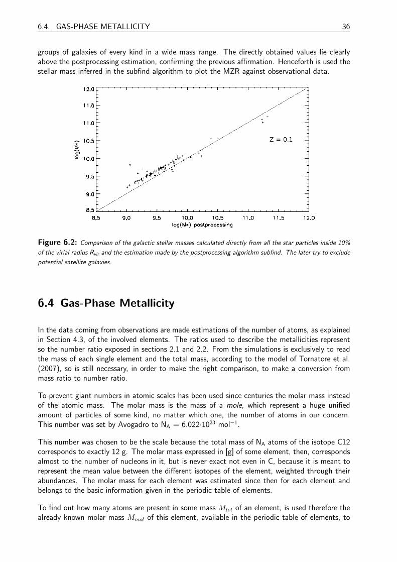
6.4. GAS-PHASE METALLICITY 36
groups of galaxies of every kind in a wide mass range. The directly obtained values lie clearlyabove the postprocessing estimation, confirming the previous affirmation. Henceforth is used thestellar mass inferred in the subfind algorithm to plot the MZR against observational data.
Figure 6.2: Comparison of the galactic stellar masses calculated directly from all the star particles inside 10%
of the virial radius Rvir and the estimation made by the postprocessing algorithm subfind. The later try to exclude
potential satellite galaxies.
6.4 Gas-Phase Metallicity
In the data coming from observations are made estimations of the number of atoms, as explainedin Section 4.3, of the involved elements. The ratios used to describe the metallicities representso the number ratio exposed in sections 2.1 and 2.2. From the simulations is exclusively to readthe mass of each single element and the total mass, according to the model of Tornatore et al.(2007), so is still necessary, in order to make the right comparison, to make a conversion frommass ratio to number ratio.
To prevent giant numbers in atomic scales has been used since centuries the molar mass insteadof the atomic mass. The molar mass is the mass of a mole, which represent a huge unifiedamount of particles of some kind, no matter which one, the number of atoms in our concern.This number was set by Avogadro to NA = 6.022·1023 mol−1.
This number was chosen to be the scale because the total mass of NA atoms of the isotope C12corresponds to exactly 12 g. The molar mass expressed in [g] of some element, then, correspondsalmost to the number of nucleons in it, but is never exact not even in C, because it is meant torepresent the mean value between the different isotopes of the element, weighted through theirabundances. The molar mass for each element was estimated since then for each element andbelongs to the basic information given in the periodic table of elements.
To find out how many atoms are present in some mass Mtot of an element, is used therefore thealready known molar mass Mmol of this element, available in the periodic table of elements, to

37 CHAPTER 6. CHEMICAL ENRICHMENT OF GALAXIES IN MAGNETICUM
get first the number of moles Nmol in this mass
Mtot = Nmol ·Mmol (6.2)
To the mass ratio obtained from the simulations is therefore needed the following transformationusing equation 6.2:
NO
NH
=MO
MH
· Mmol(H)
Mmol(O)(6.3)
The mass of each element divided by its molar mass throws the number of moles and the ratioof moles is also the ratio of atoms.
The total mass of O and H within a galaxy is calculated by adding the contribution of each singlegas particle of interest. Afterwards, is calculated the number ratio according to Equation 6.3 andfinally applied the definition of gas-phase metallicity given in Equation 2.1.
The gas-phase metallicity obtained through this method fit the observations for redshift 0 butdoesn’t show evolution, probably because of being the representation of a mean value among theall gas within the galaxy and not the recently enriched regions.
The same procedure is then applied to find the Fe abundance in the youngest stars and transformthe values to gas-phase metallicity, as explained in Section 4.3.3, which represents the last stagesof enrichment in the gas and makes possible the view of evolution.
The initial mass of star particles depends on the mass of the progenitor gas particle and both ofthem are moreover variable. As can be seen in Table 6.2, the starting mass of a gas particle inunits of M is 1.4·108 in HR resolution and 7.3·106 in UHR. Each gas particle can produce until4 star particles, so, statistically is taken a fourth of the initial mass of gas particles as a referencefor the mass of star particles, that is around 0.35·108 in HR and 1.9·106 in UHR, respectively, inunits of M.
A BH in the center of the galaxy is produced with 1000 star particles, i.e. a stellar mass of around0.35·1011 M in HR resolution and 1.9·109 M in UHR. That correspond in the logarithmic massscale to ∼ 10.5 and ∼ 9.3, respectively.
In the aim of appreciate the limits of the mass resolution and their effects in the mass-metallicityrelation (MZR), in Figure 6.3 are shown the metallicities in a wider mass range to show thebehavior of the data beyond the tentative limit of mass resolution. The best bin choice to geta picture that is dense enough to note clearly the distribution of the data along the used massrange, was the separation in bins of 0.1 dex with maximal 100 galaxies per bin.
The comparison is done with observations at redshift z ∼ 2, where is still enough massive spiralgalaxies to cover generous the range of the HR resolution. The little amount of massive spiralgalaxies at redshift zero responds probably to the big merger events that already have takenplace.
In HR resolution is achieved a very good agreement, while in UHR resolution the behavior matchthe observations but with slightly higher values, evidencing the sensitivity to the used resolutionshown in Section 6.2. The higher star formation (SF) that takes place in UHR resolution is

6.4. GAS-PHASE METALLICITY 38
Figure 6.3: Gas-phase metallicity in MAGNETICUM in comparison with the observational data from Sanders
et al. (2015) at redshift z ∼ 2, showing with a vertical dashed line the limit of the mass resolution, for HR
resolution in the top panel and for UHR resolution in the bottom panel. Each black point represents a galaxy
from the simulation.

39 CHAPTER 6. CHEMICAL ENRICHMENT OF GALAXIES IN MAGNETICUM
evidenced also in the higher values obtained in the MZR. If no further specification is given, isused the simulation in Box3 with HR resolution level.
The curve falls below the limit indicated with the dashed line. The fall is just a bit moreaccelerated than the one of the observational data, but they don’t keep any relation anyway. Thereason of the metallicity decay with the lack of resolution lies by the also lack of physics necessaryfor SF activity. In galaxies below the resolution limit are probably just a handful of gravitationalbounded particles, recognized for the subfind algorithm as a subhalo. The density of particleshere is again not enough neither to trigger enough SF nor to boost a characteristic interactionin a SF region.
6.4.1 Evolution
The key to understand the observation of evolution lies in the principles of the young stellarmetallicity method, explained in Section 4.3.3. In this method are selected the newest stars of agalaxy to infer the gas-phase metallicity in a very last stage of the galaxy, namely when these starswere born. This method is not just free of the possible systematic errors by observing the galacticnebulae, but show precisely the abundances in the star forming regions. Any other discriminationof the gas particles in simulations doesn’t take in account if this particle was enriched lately orin an early stage. The key to select the galactic regions suitable for compare with observationaldata doesn’t lie in the features of the ISM gas, but in the recent stellar activity.
The stellar metallicity of all star particles younger than 100 Myr was averaged and then trans-formed to gas-phase metallicity, following the transformation of Bresolin et al. (2016) presentedin Section 2.2. The results show in fact the newest metallicity values of each galaxy and a clearevolution with redshift.
Figure 6.4 shows the evolution from redshift z ∼ 2.3 to redshift z ∼ 0 with bins of 0.1 dex and1000 galaxies per bin, to appreciate at the best the distribution of the data. The median of thevalues is also shown, with an amazing concordance with the observational data.
6.5 Stellar Metallicity
The mass of Fe and H and the respective number ratio, needed to represent the stellar metallicityas shown in Section 2.2, is obtained in the same way as the O/H ratio for the case of the gas-phasemetallicity. In this case is not added up all the content in the galaxy before to apply Equation2.2, but calculated the number ratio for each star particle and then the mean value, since thestellar metallicity represent the mean metallicity of the stars within the galaxy.
Remarkable is that each star particle is not a single star, but a star population, limited bythe space- and mass-resolution of the simulations. Nevertheless, all stars in the population aresupposed to have the same age and initial metallicity. So is made the approximation that themetallicity of the star particle represents a mean value between the stars that belong to thepopulation.
In Figure 6.5 is shown the mass-metallicity relation (MZR), like in the case of gas-phase metallicity,
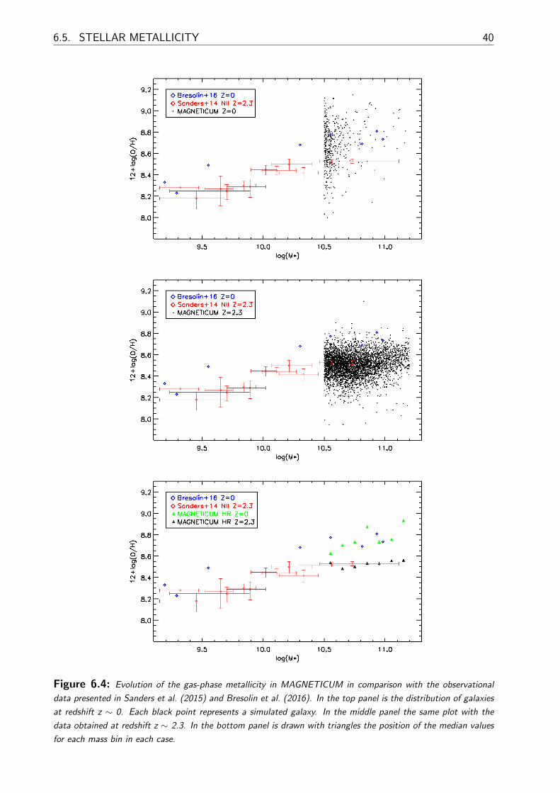
6.5. STELLAR METALLICITY 40
Figure 6.4: Evolution of the gas-phase metallicity in MAGNETICUM in comparison with the observational
data presented in Sanders et al. (2015) and Bresolin et al. (2016). In the top panel is the distribution of galaxies
at redshift z ∼ 0. Each black point represents a simulated galaxy. In the middle panel the same plot with the
data obtained at redshift z ∼ 2.3. In the bottom panel is drawn with triangles the position of the median values
for each mass bin in each case.

41 CHAPTER 6. CHEMICAL ENRICHMENT OF GALAXIES IN MAGNETICUM
for HR and UHR resolution, showing the limits of the mass resolution. As can be seen in thepicture, there are more problems reproducing the slope of the stellar MZR. In general appears tooflat in comparison to the observations. The generally flat and thin scatter of the stellar metallicitymakes moreover meaningless a separated analysis between spirals and ellipticals galaxies, whichcan be found in observational data.
Like in the case of gas-phase metallicity, the fall of the metallicities in HR resolution is moredramatic. In UHR resolution the values are just slightly higher. The difference is smaller than forthe gas-phase metallicity, probably because not all the metals overpolluting the IGM are translatedin the metallicity of the new built stars.
6.6 Gas-Phase Gradients
To make a proper comparison of the gradients with observational data is necessary to calculatefirst the effective radius Reff of each galaxy, the scale radius selected by the most observationsof gradients. In this concern, all selected particles within a galaxy were ordered with increasingradius. Then, the masses were added until to reach the half of the total stellar mass. Thecorresponding radius at this point represents Reff. As Reff is therefore taken the radius at whichthe half of the stellar mass is contained, within the 10% of the virial radius Rvir, previous selected.
For making the gradients, the metallicity at each radial position is averaged between manygalaxies. It was shown to give the best picture a configuration of 100 radial bins per Reff.
The comparison is made with the observational data from Sanchez-Menguiano et al. (2016),showed in Figure 3.1, where the metallicities are estimated with the O3N2 method. The con-versions offered in Kewley and Ellison (2008) are applicable only in a lower mass range than theexposed in this gradient. For high masses, nevertheless, The NII calibration as well as the O3N2calibration are close enough to the more reliable young stellar metallicity method, as explained inmore detail in Bresolin et al. (2016). The comparison can be seen in Figure 4.4.
This analysis is made in Box4 and UHR resolution to exploit the space resolution needed toexamine the radial range and learn so much as possible about the behavior of the gradients outof the simulations, and knowing the concordance in the behavior of the mass-metallicity relation(MZR) and just slight higher values for UHR resolution.
The radial profiles are first calculated for the whole radial range to appreciate the limitations ofthe resolution, this time of the space resolution. As can be seen in Table 6.2, the softening lengthfor gas particles in UHR resolution is 1.4 kpc/h. Considering this, the 2 innermost kpc are takenas not trustable for the tests.
Figure 6.6 shows two versions to be compared. The first version removes the 2 innermost kpcthat are not to trust for UHR resolution and the second version take all particles and indicatesthe mean position of the 2 kpc limit, since the radial profile is normalized to the Reff. The spaceresolution limitation doesn’t show a big impact like the one of mass resolution.
Figure 6.7 shows the radial profile leaving the 2 innermost kpc away, corresponding to the spaceresolution constraint, but also making the same mass bins separation as in the Graphic fromSanchez-Menguiano et al. (2016). The lower metallicities in the mass region that includes the

6.6. GAS-PHASE GRADIENTS 42
Figure 6.5: Stellar metallicity in MAGNETICUM in comparison with the observational data of all kind of
galaxies taken from Gonzalez Delgado et al. (2014) at redshift z = 0, showing with a vertical dashed line the limit
of the mass resolution. Each black point represents a simulated galaxy. In the top panel for HR resolution and in
the bottom panel for UHR resolution.
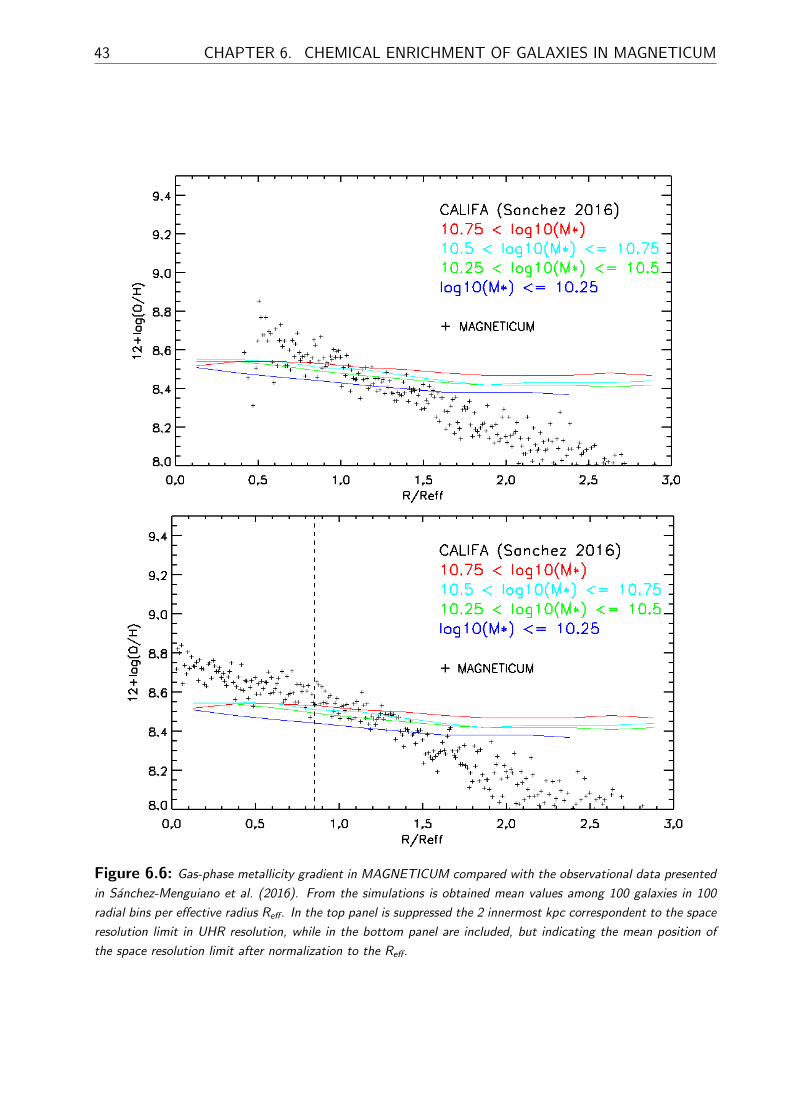
43 CHAPTER 6. CHEMICAL ENRICHMENT OF GALAXIES IN MAGNETICUM
Figure 6.6: Gas-phase metallicity gradient in MAGNETICUM compared with the observational data presented
in Sanchez-Menguiano et al. (2016). From the simulations is obtained mean values among 100 galaxies in 100
radial bins per effective radius Reff. In the top panel is suppressed the 2 innermost kpc correspondent to the space
resolution limit in UHR resolution, while in the bottom panel are included, but indicating the mean position of
the space resolution limit after normalization to the Reff.

6.6. GAS-PHASE GRADIENTS 44
region of the simulation with lack of mass resolution are evident. For the rest of mass bins thebehavior is as expected from the MZR, with the most massive galaxies showing higher values.Each mass bin keep the original slope, discarding any possibility of being the mass mixture thereason for the steeper slope.
Figure 6.7: Gas-phase Metallicity Gradient obtained in MAGNETICUM, compared with the observational data
from Sanchez-Menguiano et al. (2016). The colors indicated in the graphic correspond to the mass region for the
fits from the observations, as well as for the simulation radial bins.
As expected from the behavior of the MZR and also observed, the more massive the galaxiesare, the higher metallicities they show. A clear averaged slope is also shown, when they arenormalised through the Reff, confirming the good choice predicted theoretically and used tonormalize observational data. The gradients are in general steeper than the observed ones. Moremetals are placed near the core of the galaxies and less in the outskirts, probably because of theeffect of strong galactic winds at higher radii. The most massive bin sinks strongly in the innerregion. Possible reasons for these behaviors are discussed in Section 7.
Further tests were done, in order to find out a possible needed constraint not taken in accountfor a reasonable comparison. Observations of gas-phase metallicities are done in HII regionscharacterized for reaching a temperature of around 104 K and a minimal abundance of H of about70%. This conditions are added to the selection constraints of the ISM gas in the simulationsand compared with the observational data shown in Figure 3.1. These tests are done using theversion that leaves out the 2 innermost kpc related to the space resolution in UHR. Figure 6.8shows the results.
Warmer gas was expected to contain more metals, since the warm regions in the IGM are thoughtto gain their mass and energy mostly from close recent stellar activity, being more enriched thanthe rest of the environment. The results confirm that clearly too warm gas is newly enriched andthrow a chaotic behavior with high enriched values, while the cold gas version is more alike tothe version with no temperature constraint. The condition of high H abundance sinks the innerregion of the gradient, probably because the longer SF activity that consumed the ISM gas nearthe center of the galaxy. The mixed constraints don’t show a special feature.

45 CHAPTER 6. CHEMICAL ENRICHMENT OF GALAXIES IN MAGNETICUM
Figure 6.8: Top left: Gas-phase metallicity gradient in MAGNETICUM by taking just gas above 104 K in
comparison with the observational data from Sanchez-Menguiano et al. (2016). Around this temperature should
be reached in HII ionised regions, where observations of gas-phase metallicities take place. Top right: Same
comparison, but with gas below this temperature. Bottom left: behavior of the gradient by just taking the gas
with a composition of minimal 70% of H, which is expected in HII regions. Bottom down: A mixture constrain
between cold enough and and H rich ISM gas.
6.7 Stellar Gradients
In comparison with the gas-phase metallicity, the stellar metallicity obtained from the simulationsreproduce very well the observed gradients. We use the simulations with HR resolution in thefollowing analysis, to the detriment of the space resolution, using this to make a comparison asclose as possible with the observational data.
The softening length for star particles in HR resolution reaches 2 kpc/h, as shown in Table 6.2.The same test is made for stellar gradients taking this time also 2 kpc as tentative limit of spaceresolution.
Figure 6.9 shows the results. The discrepancies between the observations and the simulatedprofiles start by the vertical dashed line that indicates the limit of the space resolution. Thisshows how in this case, where the gradient is well reproduced, the space resolution does play arole. The version leaving out the stars in the 2 innermost kpc is still not free of values under theexpected mean values, but shows less population in this region. Probably a bigger constraint isneeded. Some authors point out a region of confidence starting by 3 times the softening length.
Figure 6.10 shows the dispersion obtained in the stellar metallicity gradients with 1, 10 and 100galaxies. The dispersion is nearly the same for every galaxy and reaches between 0.3 and 0.6 dex.The higher the number of galaxies, the regular the mean values per radial bin becomes, as well

6.7. STELLAR GRADIENTS 46
Figure 6.9: Stellar metallicity gradient in MAGNETICUM compared with the observational data presented
in Sanchez-Menguiano et al. (2016). From the simulations is obtained mean values among 100 galaxies in 100
radial bins per effective radius Reff. In the top panel is suppressed the 2 innermost kpc correspondent to the space
resolution limit, while on the bottom panel are included, but indicating the mean position of the space resolution
limit after normalization to the Reff.

47 CHAPTER 6. CHEMICAL ENRICHMENT OF GALAXIES IN MAGNETICUM
as the curve of the median values becomes, but without to change the total dispersion.
Figure 6.10: Dispersion seen in the stellar metallicity gradients in MAGNETICUM. In the left panels are shown
the gradients with the usual bining of 100 bins per effective radius Reff, while in the right panels are shown the
curve of the median values, by using only 5 bins per Reff, with error bars representing the dispersion with 15%
and 85% percentiles. Top: examples with 1 galaxy. Middle: 10 galaxies. Bottom: 100 galaxies.
Interesting to notice is how, while the mean values lie slightly below the observed ones, themedian values lie above. The latter means that although the most stars have metallicities a bitover the observed values, the metal poor outsiders are more extreme, and the responsible for theslightly mean lower enrichment seen in the stellar mass-metallicity relation (MZR).
In Figure 6.11 is shown the stellar metallicity gradients of four elliptical galaxies. The gradientused in this work for comparison, from La Barbera et al. (2012), represent a good mean behaviorfor these galaxies. From these samples, moreover, can be taken typical dispersion values atradius 1, 2 and 3 Reff by comparing the extreme values, and they match the obtained dispersionin MAGNETICUM between 0.3 and 0.6 dex, showed in Figure 6.10.

6.7. STELLAR GRADIENTS 48
Figure 6.11: Stellar metallicity gradients from the four elliptical galaxies indicated in the respective panel,
taken from Pastorello et al. (2014). In the top sub panels are represented the radial profiles inferred from the study,
normalized to the effective Radius Reff and absolute. In the lower subpanels are indicated with square symbols the
position of the measurements, color coded according to the metallicity and with a size inversely proportional to
the associated uncertainty. The pixel fill of the region is the result of the interpolation of the measurements. The
galaxies are not face-on, reason why the gradient in the minor axis appears steeper. The dashed lines represent
hereby the galaxy isophotes with circularized radius R = 1, 2 and 3 Reff. The red circles added in this work,
indicate the extreme values that appear in the outskirts and don’t follow the trend, representing probably members
of satellite galaxies or outsiders.

49 CHAPTER 6. CHEMICAL ENRICHMENT OF GALAXIES IN MAGNETICUM
6.8 behavior of Further Elements in Stars
It was also a goal to look at the behavior of further individual elements produced with thischemical enrichment model. In Ryde et al. (2016) are presented measurements with the verylarge telescope (VLT) of Mg/H and Si/H stellar metallicity ratio against the common Fe/H ratioat 100, 200 and 300 kpc galactocentric distance in the Milky Way (MW). The MW has ∼ 700pc until its effective radius Reff, so in this work is made a comparison with simulated MW-likegalaxies until 3/7 Reff.
In Ramırez et al. (2013) is made a similar analysis with the O/Fe ratio. In that work is madethe separation between thin disc and thick disc. The thin disc of the galaxy is where the starformation (SF) is higher. The most stars and also the youngest, are placed in the thin disc. Thethick disc go farther away and has older stars. There is still no way to do such a difference in asimulation specialized in cosmological resolution levels, but the positions of both curves still workas a guide for the general behavior.
In Figure 6.12 are shown the results. The observational data represent values of individual stars,while the data from the simulation represents the mean values between all stars in MW-likegalaxies placed until 3/7 of their Reff, separated in Fe/H bins.
The results in all three cases are similar. There is a clear trend in all similar plots of increasing theindividual elements abundance for under solar values of Fe/H. That means that the decrease ofFe abundance, mostly by increasing the galactocentric distance, is steeper in the case of Fe thanin the case of typical elements produced by SNII. This distribution, explained in more detail inSection 3.2, is even more emphatic at bigger scales. In the simulations, however, this distributionis not well reproduced. This reveals how the abundance profiles of other typical SNII products,like the ones of O presented in Section 6.6, are also steeper than the observed ones.

6.8. BEHAVIOR OF FURTHER ELEMENTS IN STARS 50
Figure 6.12: Top and Middle: The indicated relations presented in Ryde et al. (2016) for Mg and Si abundances
in stars, respectively, in comparison with the MAGNETICUM flat behavior. Bottom: Similar analysis with the
observational data presented in Ramırez et al. (2013) for O.

51 CHAPTER 7. DISCUSSION
7 Discussion
In Chapter 2 is described the evolution of the mass-metallicity relation (MZR) as we can learnfrom observations. From the evolution of the enrichment alone, we gain a global picture of galaxyevolution, also supported for several observables. The fact that the slope of the MZR flattenwith the time, points to an early galaxy growth through merging of small systems with low starformation (SF). A stronger SF and metallicity evolution occurs only later when the ensemblesare big enough, enriching also the environment where other small galaxies live, accelerating theirenrichment with more metals inflow. In the high mass end instead, there is an evident slowerincrement of the enrichment, since galaxies end up reaching the quenching stage, where they runout of gas to keep forming stars.
As shown in Figure 4.1, with observations out to redshift z = 2, there is a clear tendency of thestar formation efficiency (SFE) to sink with the time, always faster. How it happens cannot befully answered, but probably all galaxies end up to enter a quenching process. The scatter inthese observations is also very big, suggesting that at fixed redshift, the star formation rate (SFR)of a galaxy is strong dependent on the environment, e.g. if it is getting closer to the center ofsome cluster or victim of a big merger.
Since the awareness of the MZR it has been tried to correlate these parameters with the SFR.In general is not a good idea trying to find a MZ-SFR relation. The actual observed metallicitydepends on the entire history of gas in- and out-flow of a galaxy and the related SFR, while theactual observed SFR is only the actual one, and as shown in Santini et al. (2014), evolves withtime and with a big scatter. As found in several works (Ly et al., 2016), a dependence in theMZR on the SFR for a fixed redshift is weak, surely because of this mentioned big dispersion inthe SFR and unlucky selections of galaxies.
Only the current stellar mass is a truly good evidence of SF activity through the galactic history,including the accreted regions, and that makes the MZR the most meaningful correlation involvingmetallicity. The MZR can be seen as universal with slightly deviations dependent on the age ofvirialization of the galaxies and stronger but meaningless ones dependent on the SFR.
In this work was shown, how the discrimination of the gas by temperature or composition show nosubstantial change in the gas-phase MZR and gradients. The method proposed in Bresolin et al.(2016), and used in this work, showed that the most appropriate comparison with observationaldata is made using the time of enrichment as selection criterion. The HII observed regions areusually recently enriched regions and show the highest metallicity in the galaxy. There is no wayto extract of the simulation, at which moment a gas particle was enriched, making the youngstellar metallicity method the most appropriate to estimate gas-phase metallicities.
Thanks to this improvement in the analysis and the power of the MAGNETICUM simulations,this work shows the first simulated evolution in the MZR that reproduce the observations in therange z = 0-2.
52
Observationally, this young stellar metallicity method is the best method to find the gas-phasemetallicity in nearby galaxies, where is possible to measure the metallicity out of the stars. Forhigher redshifts are the NII and O3N2 strong-line methods recommended, which fit at the bestthis method, at least by the high mass end.
A possible scenario to explain the flatness of the stellar metallicities can be put down to the roleof the initial mass function (IMF) in the enrichment model of Tornatore et al. (2007). The use ofthe IMF to approximate the effects of stellar activity is widely spread because the impossibility toresolve single stars with the actual resolution power. An apparent good immediate approximationis achieved, but the procedure can have consequences in long term.
Through the IMF is decided how many massive stars are ready for a supernova (SN) explosionwithin a stellar population. The most massive stars end up first as SNII, while a SNIa takes longerto happen. When a SNII takes place, the amount of lost mass is reduced from the star particle,hence from the whole stellar population. In a next time step, the IMF is estimated for the wholepopulation again with the new mass and the number of stars is reduced for each region and notonly for the mass region where a group of stars was actually reduced, reducing the contributionof less massive stars and the products of SNIa. The bigger and the older the galaxies, and themore massive the populations after a long SF process are, the higher the lost of SNIa production,maintaining a nearly flat behavior instead of increase like in the observed MZR. O (SNII product)gradients instead, appear overreached in the center of the most massive galaxies.
In addition, according to observations, the behavior of the IMF in the local universe seems tovary by crossing the threshold of 1 M. As exposed in Tornatore et al. (2007), some argumentssuggest that this typical scale value could be heavier in the past, making the form of the IMFtime dependent and a source of discrepancies in the seen abundances and profiles.
The gas-phase metallicity gradient in the simulated galaxies fail in reproducing the typical flatregions seen in observations. Radial migration is a proposed theory to explain the flatness. Ifradial migration is responsible for this behavior in the profiles, then is a feature that is not wellsimulated and an interesting subject of test in future analysis.
The steeper O abundances, as well as the similar behavior of other SNII products in comparisonto Fe, are probably caused because too strong winds at higher radii. Close to the center instead,looks overreached, and the total metallicity match the observational data. If the winds throwaway the metals at higher radii more effective than one could wish, than was the process also moreeffective in early times, when there were smaller galaxies in average, overpolluting the IGM. Thisoverpollution, also reported in other similar simulations, could be the reason of the overenrichmentin the inner region, since the galaxies formed in an already overenriched environment. The resultof this scenario is a global reasonable metallicity with steeper gas-phase metallicity gradients.
Fe in the other hand, is not expelled by AGB-winds and in general less distributed and affected bythem, which is probably the reason why the stellar metallicity gradients are very well reproduced.Thanks to the MZR and the obtained gradients are found the possible improvements in thefeedback models, learning about them and building an even more powerful tool to further studies.
There are still issues to solve with the galactic feedback models to achieve results, resolutionindependent in this single case, but in general much to test and constraints to do for the future,in order to reproduce all the observables that reveal galactic evolutionary processes.

53 CHAPTER 7. DISCUSSION
Bird et al. (2016) show how the increment of the energy in SN models, using the Illustris simula-tion, helps to fit profiles of C obtained from absorption lines in quasars. The increment of energyin the winds can be achieved incrementing its speed, but that reduces at the same time the SFE.It is shown how transforming a part of the energy in heat, instead of acceleration, is achieved abetter fit in the profiles without to disturb the SF activity. Nevertheless, this improvement justreproduce good the observations around low-mass haloe and not around big massive objects. Itwas proposed to change the AGN feedback model for further chemical enrichment without towarm the gas too much. We can learn from these cases how inaccurate the used feedback modelsstill are, by reproducing universally a wide range of galaxies. The energy and mass produced byall the galactic feedback processes are intrinsic connected and the way they manifest, as well asthe interplay between them, has to be still better understood.

References 54
References
Andrews, B. H. and Martini, P. (2013). The Mass-Metallicity Relation with the Direct Method onStacked Spectra of SDSS Galaxies. Astrophysical Journal, 765:140.
Bird, S., Rubin, K. H. R., Suresh, J., and Hernquist, L. (2016). Simulating the carbon footprint ofgalactic haloes. Monthly Notices of the RAS, 462:307–322.
Borgani, S. et al. (2008). The Chemical Enrichment of the ICM from Hydrodynamical Simulations.Space Science Reviews, 134:379–403.
Bresolin, F. et al. (2016). Young stars and ionized nebulae in M83: comparing chemical abundances athigh metallicity. ArXiv e-prints.
Bruzual, G. and Charlot, S. (2003). Stellar population synthesis at the resolution of 2003. MonthlyNotices of the RAS, 344:1000–1028.
Chiosi, C., Merlin, E., and Piovan, L. (2012). The Origin of the Mass-Radius Relation of Early-TypeGalaxies. ArXiv e-prints.
Davee, R., Finlator, K., and Oppenheimer, B. D. (2006). The Mass-Metallicity Relation in CosmologicalHydrodynamic Simulations. ArXiv Astrophysics e-prints.
Denicolo, G., Terlevich, R., and Terlevich, E. (2002). New light on the search for low-metallicity galaxies- I. The N2 calibrator. Monthly Notices of the RAS, 330:69–74.
Erb, D. K. et al. (2006). The Mass-Metallicity Relation at z > 2. Astrophysical Journal, 644:813–828.
Gallazzi, A. et al. (2005). The ages and metallicities of galaxies in the local universe. Monthly Noticesof the RAS, 362:41–58.
Gonzalez Delgado, R. M. et al. (2014). Insights on the Stellar Mass-Metallicity Relation from theCALIFA Survey. Astrophysical Journal, Letters, 791:L16.
Hirschmann, M. et al. (2015). The stellar accretion origin of stellar population gradients in massivegalaxies at large radii. Monthly Notices of the RAS, 449:528–550.
Jimmy et al. (2015). The Gas Phase Mass Metallicity Relation for Dwarf Galaxies: Dependence on StarFormation Rate and H I Gas Mass. Astrophysical Journal, 812:98.
Kewley, L. J. and Ellison, S. L. (2008). Metallicity Calibrations and the Mass-Metallicity Relation forStar-forming Galaxies. Astrophysical Journal, 681:1183–1204.
La Barbera, F. et al. (2012). SPIDER - VII. Revealing the stellar population content of massive early-typegalaxies out to 8Re. Monthly Notices of the RAS, 426:2300–2317.
Lequeux, J. et al. (1979). Chemical composition and evolution of irregular and blue compact galaxies.Astronomy and Astrophysics, 80:155–166.

55 References
Lonoce, I. et al. (2015). Old age and supersolar metallicity in a massive z ∼ 1.4 early-type galaxy fromVLT/X-Shooter spectroscopy. Monthly Notices of the RAS, 454:3912–3919.
Ly, C., Malkan, M. A., Rigby, J. R., and Nagao, T. (2016). The Metal Abundances across CosmicTime (MACT) Survey. II. Evolution of the Mass-Metallicity Relation over 8 Billion Years, Using[OIII]4363AA-based Metallicities. Astrophysical Journal, 828:67.
Ma, X. et al. (2016). The origin and evolution of the galaxy mass-metallicity relation. Monthly Noticesof the RAS, 456:2140–2156.
Maiolino, R. et al. (2008). AMAZE. I. The evolution of the mass-metallicity relation at z > 3. Astronomyand Astrophysics, 488:463–479.
Naab, T., Johansson, P. H., and Ostriker, J. P. (2009). Minor Mergers and the Size Evolution ofElliptical Galaxies. Astrophysical Journal, Letters, 699:L178–L182.
Pastorello, N. et al. (2014). The SLUGGS survey: exploring the metallicity gradients of nearby early-typegalaxies to large radii. Monthly Notices of the RAS, 442:1003–1039.
Peng, Y., Maiolino, R., and Cochrane, R. (2015). Strangulation as the primary mechanism for shuttingdown star formation in galaxies. Nature, 521:192–195.
Pettini, M. and Pagel, B. E. J. (2004). [OIII]/[NII] as an abundance indicator at high redshift. MonthlyNotices of the RAS, 348:L59–L63.
Ramırez, I., Allende Prieto, C., and Lambert, D. L. (2013). Oxygen Abundances in Nearby FGK Starsand the Galactic Chemical Evolution of the Local Disk and Halo. Astrophysical Journal, 764:78.
Ryde, N. et al. (2016). Chemical Evolution of the Inner 2 Degrees of the Milky Way Bulge: [α/Fe]Trends and Metallicity Gradients. Astronomical Journal, 151:1.
Sanchez-Blazquez, P. et al. (2014). Stellar population gradients in galaxy discs from the CALIFA survey.The influence of bars. Astronomy and Astrophysics, 570:A6.
Sanchez-Menguiano, L. et al. (2016). Shape of the oxygen abundance profiles in CALIFA face-on spiralgalaxies. Astronomy and Astrophysics, 587:A70.
Sanders, R. L. et al. (2015). The MOSDEF Survey: Mass, Metallicity, and Star-formation Rate at z ∼2.3. Astrophysical Journal, 799:138.
Santini, P. et al. (2014). The evolution of the dust and gas content in galaxies. Astronomy andAstrophysics, 562:A30.
Sato, K., Matsushita, K., and Gastaldello, F. (2009). Temperature and Metallicity in the Intra-ClusterMedium of Abell 262 Observed with Suzaku. Publications of the ASJ, 61:S365–S376.
Simionescu, A. et al. (2009). Chemical enrichment in the cluster of galaxies Hydra A. Astronomy andAstrophysics, 493:409–424.
Springel, V. and Hernquist, L. (2003). Cosmological smoothed particle hydrodynamics simulations: ahybrid multiphase model for star formation. Monthly Notices of the RAS, 339:289–311.
Steidel, C. C. et al. (2014). Strong Nebular Line Ratios in the Spectra of z ∼ 2-3 Star Forming Galaxies:First Results from KBSS-MOSFIRE. Astrophysical Journal, 795:165.
Steven, W. S. and Palla, F. (2008). The Formation of Stars. WILEY-VCH Verlag GmbH & Co. KGaA.

References 56
Tornatore, L., Borgani, S., Dolag, K., and Matteucci, F. (2007). Chemical enrichment of galaxy clustersfrom hydrodynamical simulations. Monthly Notices of the RAS, 382:1050–1072.
Tremonti, C. A. et al. (2004). The Origin of the Mass-Metallicity Relation: Insights from 53,000Star-forming Galaxies in the Sloan Digital Sky Survey. Astrophysical Journal, 613:898–913.
Yabe, K. et al. (2015). The Subaru FMOS Galaxy Redshift Survey (FastSound). III. The mass-metallicityrelation and the fundamental metallicity relation at z ∼ 1.4*. Publications of the ASJ, 67:102.
Zahid, H. J. et al. (2014). The FMOS-COSMOS Survey of Star-forming Galaxies at z ∼ 1.6. II.The Mass-Metallicity Relation and the Dependence on Star Formation Rate and Dust Extinction.Astrophysical Journal, 792:75.


58
Affirmation
I declare with this, I wrote this work on my own and I used no other sources and aids than thosegiven in this work.
Munich, November 2016
Emilio Mevius