capabilities of chemical simulation methods in the

1195

Pure Appl. Chem., Vol. 80, No. 6, pp. 1195–1210, 2008.doi:10.1351/pac200880061195© 2008 IUPAC

Capabilities of chemical simulation methods inthe elucidation of structure and dynamics ofsolutions*

Thomas S. Hofer‡, Andreas B. Pribil, and Bernhard R. Randolf

Theoretical Chemistry Division, Institute of General, Inorganic and TheoreticalChemistry, University of Innsbruck, Innrain 52a, A-6020 Innsbruck, Austria

Abstract: As a result of recent methodological developments in connection with enhancedcomputational capacity, theoretical methods have become increasingly valuable and reliabletools for the investigation of solutions. Simulation techniques utilizing a quantum mechani-cal (QM) approach for the treatment of the chemically most relevant region so-called hybridquantum mechanical/molecular mechanical (QM/MM) simulations have reached a level ofaccuracy that often equals or may even surpass experimental methods. The latter is true inparticular whenever ultrafast (i.e., picosecond) dynamics prevail, such as in labile hydrates orstructure-breaking systems.

The recent development of an improved QM/MM framework, the quantum mechanicalcharge field (QMCF) ansatz, enables a broad spectrum of solute systems to be elucidated. Asthis novel methodology does not require any solute solvent potential functions, the applica-bility of the QMCF method is straightforward and universal. This advantage is bought, how-ever, at the price of a substantial increase of the QM subregion, and an attendant increase incomputational periods to levels of months, and even a year, despite parallelizing high-per-formance computing (HPC) clusters.

Molecular dynamics (MD) simulations of chemical systems showing increasing com-plexity have been performed, and demonstrate the superiority of the QMCF ansatz over con-ventional QM/MM schemes. The systems studied include Pd2+, Pt2+, and Hg2

2+, as well ascomposite anions such as PO4

3– and ClO4–.

Keywords: QM/MM MD simulation; QMCF MD simulation; ion solvation; hydration struc-ture; hydration dynamics.

INTRODUCTION

The field of solution chemistry has gained an increasingly important position in chemical research[1–4], as the liquid state is by far the most relevant one in chemistry and also of great importance in re-lated disciplines such as physics, biology, and geology. For this reason, solution chemistry is not re-stricted to an exclusive part of chemistry—the majority of chemical reactions and basically all biolog-ical processes take place in liquid phase and are strongly dependent on the properties of the solvent andits interaction with all present species. Typical solvate systems range from ionic hydrates, inorganic andmetal–organic complexes, and (bio)organic molecules to macromolecules such as nucleic acids, pro-

*Paper based on a presentation at the 30th International Conference on Solution Chemistry (ICSC 30), 16–20 July 2007, Perth,Australia. Other presentations are published in this issue, pp. 1195–1347.‡Corresponding author: Tel.: +43-512-507-5161; Fax: +43-512-507-2714; E-mail: [email protected]

teins, and composite membrane layers, thus covering inorganic and organic chemistry as well as bio-chemistry (which is strongly linked to pharmaceutical science) and geochemistry, including the casewhere nonambient conditions such as high temperatures or pressures act on the liquid.

The theoretical models utilized in the underlying interpretation of the experimental results dependon concepts of physical chemistry like statistical thermodynamics [5,6] and the theory of intermolecularforces [7]. This relation became more evident after the technological resources allowed a computationaltreatment of condensed chemical systems, even at the level of quantum mechanics (QM), thereby ex-panding applied theoretical chemistry to the liquid state [8–10].

As solution chemistry is a multidisciplinary field of research, a variety of experimental as well astheoretical methods are being employed to investigate solvation processes. Methods relying on X-rayradiation and neutron beams have been applied to determine structural properties [1,2,11–13] whileother methods like NMR [3,14] and a variety of other spectroscopic methods enable the investigationof dynamical aspects [15–17]. One of the most active fields is the investigation of the solvation struc-ture of ions in solutions [1,3,11,14] as ionic solvates show a broad spectrum of properties and thuschemical behavior.

One of the most illustrative properties to demonstrate the diversity of ion solvation is the meanligand residence time (MRT) of first-shell ligands in aqueous solution being in the order of 300 yearsfor Ir(III) and lower than 200 ps in the case of Cs(I) [3,14], thus covering a range of 20 orders of mag-nitude. The latter value is an upper limit deduced from IQENS (incoherent quasielastic neutron scat-tering) experiments, as the actual exchanges occur too fast to be studied by presently available experi-mental techniques [3,14]. Femtosecond laser pulse spectroscopy has been applied to investigate themean lifetime of bonds and coordination in pure water, yielding a value of 2.0 ps [15], but the applica-tion of this technique to solute–solvent interactions still faces unsolved technical problems. Computersimulations [4,18,19], on the other hand, are capable of reproducing the time evolution of chemical sys-tems on a very small time scale such as the picosecond regime, and, thus, detailed investigations ofthese ultrafast ligand-exchange dynamics can be performed based on computational methods. Whereasexperimental methods study systems on the macroscopic scale and thereby automatically average themeasured properties over all species present in solution, theoretical models deal with the problem onthe microscopic, i.e., the atomic and molecular scale, respectively. This approach gives the unique op-portunity to monitor and analyze the behavior of every single molecule and atom within the system in-dependently. As liquids combine the density of solids with the mobility of a gas, an accurate descrip-tion of all interactions at this level is the key challenge determining the accuracy of simulations.

METHODOLOGIES FOR SIMULATING LIQUID SYSTEMS

It is known from statistical thermodynamics [5,6] that a single structure with a distinct distribution ofatoms is an insufficient representation of chemical systems at any temperature above 0 K. As many dif-ferent arrangements of the molecules and atoms will correspond to the same energy, a collection of rep-resentative configurations—an ensemble—is required in order to derive a reliable average descriptionof the system, thus also accounting for the influence of entropy.

The very frequently used method of the QM “geometry optimization” is an inadequate tool forthe investigation of liquid-state chemistry, as a single minimum structure does not, in general, corre-spond to any of the many representative configurations. The application of a polarizable continuummodel (PCM) [20] in the minimization procedure in order to model the potential of the surrounding sol-vent [21] has no influence on this methodical shortcoming. Moreover, PCMs represent the surroundingsolvent by a constant continuum and thus affect the calculation by a homogeneous potential. At closedistances to the solute, the distribution of the surrounding molecules can by no means be assumedhomogeneous, however. Hence, conclusions of theoretical investigations based on geometry optimiza-tions even in combination with PCMs have to be critically assessed.

T. S. HOFER

© 2008 IUPAC, Pure and Applied Chemistry 80, 1195–1210

1196

Methods suitable for collecting multiple configurations of an ensemble are known as “statisticalsimulation methods” [4,18]. Two different approaches exist, the Monte Carlo (MC) and the moleculardynamics (MD) framework. Both methodologies utilize a periodic simulation box (various shapes suchas cubes or truncated octahedrons can be employed) to ensure that the simulation corresponds to the sit-uation within bulk. In MC methods in general only a single molecule is moved per step (typically viarotation and/or translation), and the energy difference between the newly generated and the old config-uration is considered according to the Metropolis algorithm [22], determining the new configuration’sacceptance. MD methods propagate the entire system based on an integration of the Newtonian equa-tions of motions with typical time steps on the femtosecond scale and below. While MC methods re-quire the knowledge of the total energy of the system, MD simulations are based on the forces actingon all particles of the system (the total energy is only required to monitor the stability of the simula-tion). As MC simulations modify the system randomly, time-dependent properties cannot be evaluated.Nevertheless, MC methods are versatile tools as a large number of different configurations can bequickly compared, which is advantageous in investigations of large biomolecules and docking studies.

Implementations of the MC and MD frameworks are widespread today. One of the main chal-lenges determining the quality of a simulation is the achievable accuracy of energies and forces. In prac-tice, two main approaches exist—molecular mechanics (MM) and quantum mechanics (QM). MMmethods are based on parametrized functions representing the interaction between two species. TheLennard–Jones 6–12 potential plus a Coulombic term is one of the simplest potential functions available.Although the construction of the parameters defining the potentials is a difficult, tedious, and, above all,time-consuming task, the accuracy of these approaches is, in general, limited, especially when metal ionsare present in the system. Large effort has been devoted to derive better potential forms and parameters,resulting in an enormous amount of literature providing numerous different MM methodologies.

On the other hand, MM methods are computationally very cheap, which is their main advantagefor the treatment of large biomolecules such as proteins, nucleic acids, or membranes, which can onlybe achieved by MM methods to date. Entire sets of balanced parameters are known as force fields[23–25], typically parametrized to describe a certain subset of molecules, such as peptides, glycosides,nucleic acids, and membranes. Owing to the complex properties of metal centers in such systems, theirparametrization is very challenging, as many body and polarization effects are in general not coveredby MM methods, but of high relevance for the chemistry of such centers.

QM methods can overcome these problems as many body and polarization effects are automati-cally taken into account. QM methods derive energies and forces based on numerical solutions ofSchrödinger’s equation [26], which are very universal but extraordinarily time-consuming. A large hier-archy of different QM methods exists today [4,8,10] in which accuracy is modestly improving, whilethe computational demand increases exponentially. A lot of research is devoted to further improvementsof the accuracy of QM methods while keeping the associated computational demand within practicallimits. Some promising approaches have been formulated which could prove very helpful in the nearfuture [27–29].

Although commercial QM software packages enable a parallel execution of QM calculations uti-lizing high-performance computing (HPC) clusters, only a small number of particles can be treated, typ-ically up to 100, depending on the accuracy of the QM treatment.

Therefore, compromises between accuracy and computational effort have to be sought.Car–Parrinello (CP) simulations [30] achieve this compromise by employing very simple and time-sav-ing QM methods (namely, density functional theory, or DFT, on the generalized-gradient approxima-tion level such as PBE [31,32] or BLYP [33]) and by a reduction of the number of particles and the sim-ulation time to a (sometimes critical) minimum.

In different studies [34,35], CP simulations have proven to yield data in strong contrast to exper-imental as well as other theoretical investigations utilizing a more advanced and, therefore, more de-manding methodology. In many cases, the shortcomings can be explained by the severe inherentmethodical errors of common DFT methods, which have been outlined in detail in a recent report [36].


Capabilities of chemical simulation methods 1197

The reduction of the number of particles sometimes leads to simulation systems which are incapable ofeven forming a complete second solvation shell and much less, providing a sufficient number of bulkmolecules representing the surrounding solvent [37].

A lot of confusion exists with respect to a consistent nomenclature of DFT methods. Althoughmany scientists utilizing DFT methods insist on the usage of the term “ab initio” or “first principle” inconnection with DFT methods, the majority of present implementations of density functional theoryrely on a number of empirical calibrations, which is in contrast with the dogma of ab initio methods notto use any experimental or empirical data. This applies to the usage as well as to the formulation of therespective methodology, thus characterizing common DFT approaches rather as semiempirical methods[36,38–40]. Alternative approaches to formulate true ab initio DFT methods have been presented, how-ever, aiming at the elimination of the severe methodical shortcomings of present DFT implementationsand at the same time trying to avoid any calibrations [36,38,39].

Another frequently used ansatz to find a compromise between computational effort and accuracyare hybrid QM/MM methodologies (see Fig. 1) [41–46]. The chemically most relevant system (e.g., anion and its hydration shell) is treated by QM, while the remaining part of the system is treated by MM.This idea combines the accuracy of QM, namely, the inclusion of all important many-body and polar-ization effects near the solute with the affordability of MM. Basically, every affordable QM method ful-filling the accuracy requirements can be utilized to describe energy and forces in the QM region. Theevaluation of interactions between the two subregions is a challenge, especially if molecules migratefrom one zone to the other or bonds are cut by the QM/MM interface.

One critical test scenario to assess the reliability of such methods is the investigation of purewater. The QM/MM MD method was not only able to reliably predict the structural data but also verysensitive dynamical parameters—the MRT, the hydrogen bond lifetime, and the average hydrogen bondnumber—in excellent agreement with recent experimental studies [47,48]. Investigations of various hy-drated ions utilizing the QM/MM ansatz within the MD framework proved to yield reliable data [49,50]if at least double-zeta plus polarization basis sets were utilized in a Hartree–Fock-level treatment. It wasalso deduced that for some systems the inclusion of the second hydration shell into the QM region ismore advantageous than the application of a correlated QM method such as MP/2, which still restrictsthe manageable size of the QM region to the first hydration shell [47,51]. Apparently, quantum effects

T. S. HOFER


1198

Fig. 1 Scheme of a QM/MM simulation. The chemically most relevant region (indicated by the sphere) is treatedat the respective QM level, whereas the interactions in the remaining part of the simulation cube are evaluated byMM.

extending beyond the first shell are more important than the small improvements in accuracy achievedby partial inclusion of electron correlation in ion solvates.

Although a large number of simulations have proven the reliability of the QM/MM MD method-ology, a more advanced simulation method, the quantum mechanical charge field (QMCF) MD frame-work [52], was developed to further increase the accuracy, reliability, and applicability of MD simula-tions. The main increase in accuracy is achieved through an improved coupling of the subregions byinclusion of the point charges of the MM region into the QM treatment. This technique known as elec-trostatic embedding does not significantly extend the computational demand and has been utilized invarious investigations [42,53,54], therefore. A further consequence of the improved coupling formu-lated in the QMCF method is that all interactions between the solute and solvent molecules are takeninto account by the QM treatment and the respective CF interaction. Thus, basically any solute can betreated on the basis of this methodology. The number of particles of the solute plus the required num-ber of solvent molecules to hydrate the solute determine the computational effort, which is thus the onlylimiting factor in the applicability of the QMCF method.

SIMULATION RESULTS

A first example for ligand-exchange reactions is the Cs(I) ion in aqueous solution [55]. Considering theupper limit of the MRT determined by IQENS methods as 200 ps [3], it is evident that this ion is oneof the most interesting targets for such studies. Furthermore, the Cs(I) ion is being classified as a “struc-ture breaker” in literature as it is supposed to significantly perturb the water structure instead of form-ing stable hydrate complexes. Figure 2a depicts the radial distribution functions (RDFs) obtained from



Fig. 2 (a) Cs–O (solid line) and Cs–H (dashed line) RDF, (b) coordination number distribution for the first andsecond shell, and (c) distance plot for first-shell ligand exchanges obtained from a QM/MM MD simulation of Cs(I)in aqueous solution.

a 15 ps QM/MM MD simulation of Cs(I) in aqueous solution. The bond distance of the first shell of3.25 Å as well as the first-shell coordination number found as 7.8 are in good agreement with experi-mental results [56] given as 3.22–3.30 Å for the Cs–O distance and 6–7.9 for the coordination number.However, the considerably high intensity of the minimum between first and second shell indicates thata large number of ligand exchanges took place within the simulation time. The coordination numberdistributions for the first and second shell given in Fig. 2b reveal a broad distribution of species, and,hence, the value of 7.8 deduced from the RDF has to be considered as an average value. The exchangeplot depicted in Fig. 2c demonstrates the ultrafast (i.e., picosecond scale) dynamics of the ligand ex-change. During the 15 ps of the simulation, 76 exchange events lasting longer than the critical value of0.5 ps [57] were registered, resulting in an MRT of 1.5 ps. This value is slightly smaller than the MRTof pure water obtained as 1.7 ps from analogous QM/MM MD simulations [47]. Thus, it can be con-cluded that the ion accelerates the water molecules’ movements in its vicinity rather than forming a sta-ble complex, which appears to be the reason for the “structure-breaking” ability of this particular ion.The MRT value of the second shell was found to be even shorter, namely, 1.3 ps, demonstrating that thestructure-breaking effect extends to a larger region.

These findings have some implications for experimental investigations. First, the MRT value de-duced from the simulation is significantly smaller than the upper limit deduced from IQENS studies,and hence the exchange rate range for hydrated ions has to be extended from 20 orders of magnitude to22. Secondly, experimental measurements scanning a sample for a considerably longer time period thanthe MRT (i.e., hundreds of picoseconds to nanoseconds) will automatically result in an averaged speciesdistribution summarizing a number of different hydrates with varying coordination numbers and asso-ciated structures. Even if the experimental technique enables the measurement of dynamics on thesubpicosecond scale, the large number of solutes present in solution (typically in the milli- to nanomo-lar range) will produce a variety of hydrated species, as the ions in solution will show different hydra-tion structures and will not exchange ligands synchronously.

One particular advantage of simulation methods is the distinct evaluation of every configuration,thus enabling the analysis of the species distribution and their individual structures. The detailed treat-ment of even a single hydrated ion in an environment corresponding to infinite dilution enables thetreatment of the system without the influence of counterions. The challenge of simulation work, espe-cially if QM are applied, is to sample a sufficiently large number of configurations to obtain reliablestatistics for all properties of interest.

In general, high ligand-exchange rates are a challenge for experimental studies, whose detectionlimits are typically in the nanosecond region, whereas they are favorable for simulation techniques, asa sufficient number of exchanges can be monitored within a short simulation time. On the other hand,low exchange rates are difficult to evaluate by means of simulations as very long trajectories are re-quired to monitor exchange events.

Simulations of alkaline and alkaline earth ions in aqueous solution underline these conclusions.Table 1 summarizes the first-shell bond lengths, the distribution of the coordination numbers, and thefirst-shell MRTs. Except in the case of Mg(II) [58], exchange events occur on the picosecond scale, as-sociated with a multispecies distribution. In the case of Ca(II), only three exchange events were moni-tored along the simulation [59] and due to the associated uncertainty, the estimated MRT for this par-ticular system has to be considered as lower limit.

It can be seen from Table 1 that the MRT values of the alkaline earth ions Sr(II) [60] and Ba(II)[61] are one order of magnitude larger than those of the alkaline ions. Based on the simulation results,the upper limits of the exchange rates deduced from experiments [3,14] are much too high and do notenable a realistic insight into ligand-exchange processes and the properties of these ions in aqueous so-lution, therefore.

T. S. HOFER


1200

Table 1 Ion–oxygen distance r1 in Å, distributionof coordination number CN1 and MRT τ1 in ps ofthe first-shell ligands of hydrated alkaline andalkaline earth ions obtained from QM/MM MDsimulations.

Ion r1 CN1 τ1

Na(I) 2.33 4–7 2.4K(I) 2.81 6–9 2.1Rb(I) 2.95 4–10 1.9Cs(I) 3.25 5–10 1.5Mg(II) 2.05 6.0 –Ca(II) 2.46 6–9 >43Sr(II) 2.69 8–10 45Ba(II) 2.86 8–11 19

Simulations of various other systems were carried out as well in order to investigate whether first-shell ligand exchanges can be observed by means of MD simulations. In QM/MM MD studies of themonovalent ions Ag(I) [62] and Au(I) [63] and the divalent ions Hg(II) [64] and Sn(II) [65] first-shellexchanges were observed on the picosecond scale, whereas ions such as Zn(II) [66] and Pb(II) [67]were found to form stable hydrate complexes which do not exchange ligands within the picosecondscale.

A unique hydration was observed in the case of hydrated Sn(II) [65]. The Sn–O and Sn–H RDFs(cf. Fig. 3a) point toward a regular hydration structure with an average of eight ligands found at a bondlength of 2.53 Å with an MRT of 10.0 ps. A detailed analysis of the ion–oxygen bond lengths of thefirst-shell ligands (see Fig. 3d) has shown that four molecules are strongly bound and did not exchangealong the 30.0 ps trajectory, while the remaining ligands (in average, four) are exchanged rapidly withan average MRT value of 5.0 ps. An analysis of the first-shell peak of the ion–oxygen RDF as well asthe first-shell ion–oxygen spectrum showed that it is possible to fit two Gaussian peaks with separatepeak maxima. Whereas the results are not as good in the case of the ion–oxygen RDF, the fit of the cor-responding vibrational spectrum gives an unambiguous result. It has to be mentioned, though, that thefitting of Gaussian functions is a very crude method, and as the peaks show a significant overlap in bothcases the standard deviation of the fitted values has to be considered rather high. This MD investigationfavorably supplements the conclusions of Ohtaki and coworkers who have assumed four ligands atshorter bond lengths and two other ligands at larger distance, thus resulting in a total coordination num-ber of six [1]. The difference in the coordination numbers from experimental and theoretical data canbe explained by the weak bond strength of the ligands with a high exchange rate, which makes the ex-perimental analysis of these ligands difficult. The weak bonding should also be associated with a sig-nificant concentration dependence of species. The diffraction study was carried out with concentratedsolutions (molar ratio 16.8 and 12.0), which is strongly different from the conditions of the theoreticalapproach.

Pb(II) did not show any exchange of first-shell ligands [67] although one could expect a shorterfirst-shell MRT value than for Sn(II), similar to the corresponding ions of the alkaline and alkaline earthseries Cs(I) and Ba(II). The stable first-shell hydrate of Pb(II) consisting of nine ligands is character-ized, however, by inter-shell motions of the ligands. Water molecules are moving within the first hy-dration layer, but are not released to the second shell. It appears that these inter-shell migrations are sta-bilizing the entire hydrate complex and are responsible for the lower exchange rate.



A peculiar case is hydrated Cu(II) which shows a distorted first-shell structure resulting from theJahn–Teller effect [51,68,69]. The ion–water RDF (cf. Fig. 4a) indicates a stable sixfold first-shell hy-drate. Ligands in axial positions show an elongated bond, while the remaining four ligands are found ata closer distance. In contrast to Jahn–Teller distorted structures found in crystals, this effect is highlydynamical in solution. Figure 4c shows the O–O distance of opposite ligands within the hydrate com-plex. The elongation of the bond occurs for all three pairs and is continuously changing from one lig-and pair to another.

Due to these rapid variations and the arbitrary definition of the borderline between contracted andelongated positions in some configurations, the number of distant ligands is not exclusively two. As de-picted in Fig. 4c, the elongation of the O–O distances of opposite first-shell water molecules are fluc-tuating on the picosecond scale. It appears that this dynamic Jahn–Teller effect destabilizes the first-shell complex, and thus the exchange rate of the first-shell ligands of Cu(II) is significantly higher thanthat of other divalent third-row transition-metal ions [3,14]. A similar acceleration of the exchange ratefor ligands in elongated axial positions is observed in simulations of Pd(II) and Pt(II), which will be dis-cussed in more detail below.

The bond lengths resulting from the Cu(II) simulations as 1.96/2.3 Å agree well with the experi-mental values of 2.03/2.3 Å determined by an EXAFS (extended X-ray absorption fine structure) andLAXS (large-angle X-ray scattering) study [70]. The differences of the lower bond length correspon-ding to the contracted positions can be explained by the dynamics observed in solution. The rapid in-terchanges from elongated to contracted positions and vice versa influence the average value as does

T. S. HOFER


1202

Fig. 3 (a) Sn–O (solid line) and Sn–H (dashed line) RDF of Sn(II) in aqueous solution. Fit of gaussian functionsfor (b) the Sn–O RDF and (c) the Sn–O vibrational spectrum. (d) Distance plots of the four stable first-shell ligands.(e) Snapshot of the simulation.

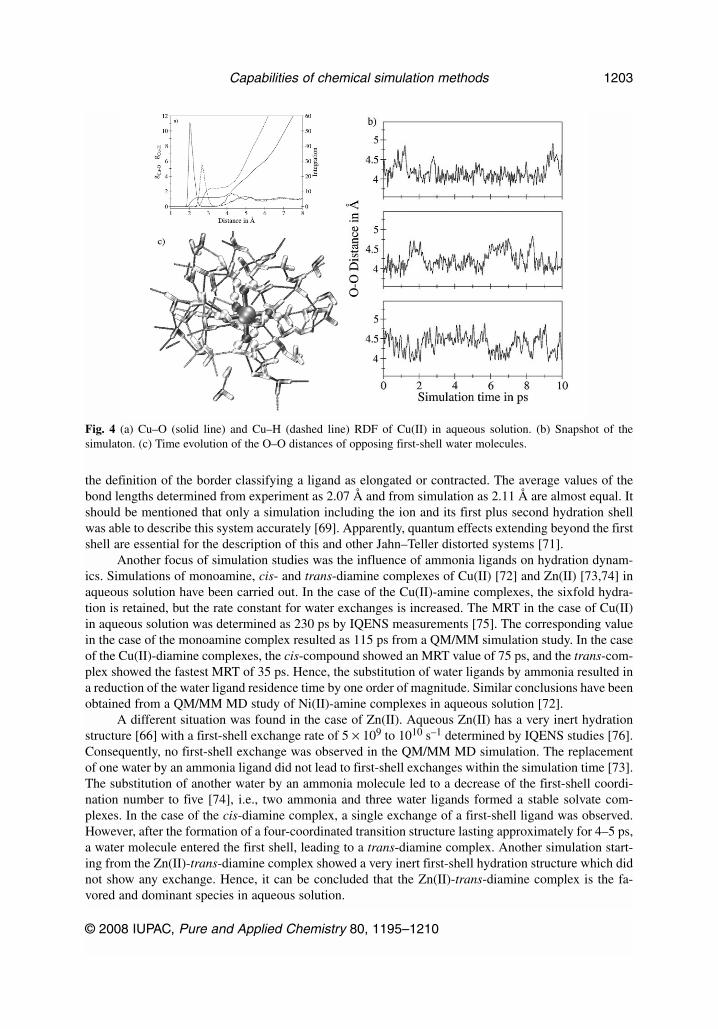
the definition of the border classifying a ligand as elongated or contracted. The average values of thebond lengths determined from experiment as 2.07 Å and from simulation as 2.11 Å are almost equal. Itshould be mentioned that only a simulation including the ion and its first plus second hydration shellwas able to describe this system accurately [69]. Apparently, quantum effects extending beyond the firstshell are essential for the description of this and other Jahn–Teller distorted systems [71].

Another focus of simulation studies was the influence of ammonia ligands on hydration dynam-ics. Simulations of monoamine, cis- and trans-diamine complexes of Cu(II) [72] and Zn(II) [73,74] inaqueous solution have been carried out. In the case of the Cu(II)-amine complexes, the sixfold hydra-tion is retained, but the rate constant for water exchanges is increased. The MRT in the case of Cu(II)in aqueous solution was determined as 230 ps by IQENS measurements [75]. The corresponding valuein the case of the monoamine complex resulted as 115 ps from a QM/MM simulation study. In the caseof the Cu(II)-diamine complexes, the cis-compound showed an MRT value of 75 ps, and the trans-com-plex showed the fastest MRT of 35 ps. Hence, the substitution of water ligands by ammonia resulted ina reduction of the water ligand residence time by one order of magnitude. Similar conclusions have beenobtained from a QM/MM MD study of Ni(II)-amine complexes in aqueous solution [72].

A different situation was found in the case of Zn(II). Aqueous Zn(II) has a very inert hydrationstructure [66] with a first-shell exchange rate of 5 × 109 to 1010 s–1 determined by IQENS studies [76].Consequently, no first-shell exchange was observed in the QM/MM MD simulation. The replacementof one water by an ammonia ligand did not lead to first-shell exchanges within the simulation time [73].The substitution of another water by an ammonia molecule led to a decrease of the first-shell coordi-nation number to five [74], i.e., two ammonia and three water ligands formed a stable solvate com-plexes. In the case of the cis-diamine complex, a single exchange of a first-shell ligand was observed.However, after the formation of a four-coordinated transition structure lasting approximately for 4–5 ps,a water molecule entered the first shell, leading to a trans-diamine complex. Another simulation start-ing from the Zn(II)-trans-diamine complex showed a very inert first-shell hydration structure which didnot show any exchange. Hence, it can be concluded that the Zn(II)-trans-diamine complex is the fa-vored and dominant species in aqueous solution.



Fig. 4 (a) Cu–O (solid line) and Cu–H (dashed line) RDF of Cu(II) in aqueous solution. (b) Snapshot of thesimulaton. (c) Time evolution of the O–O distances of opposing first-shell water molecules.

Investigations of ions in mixed solvents like water/ammonia [77–79] demonstrate another key ad-vantage of simulation methods. Figure 5 displays all RDFs between non-hydrogen atoms observed forCa(II) in aqueous ammonia [77]. It can be seen that the first-shell RDFs, especially Ca–N, Ca–O, andO–O, strongly overlap. Experimental investigations measure all of these pair distributions simultane-ously, and thus the formulation of a suitable solvation model to fit and decompose the measured data isa difficult task. Ligand exchanges leading to a variety of species being simultaneously present in solu-tion further complicate the analysis of experimental spectra. In this and similar cases, simulation meth-ods can provide valuable information for the establishment of suitable models for fitting.

The novel QMCF MD methodology [52] has the advantage that no potentials between solvent andsolute particles are required, as the associated force contributions are treated by QM and on the basisof partial charges quantum mechanically derived in every simulation step. This opens the possibility toinvestigate systems whose interactions are difficult to represent by MM potential functions. It shouldnot be concealed that the possibility to renounce solute–solvent potentials is achieved at the price of anextended QM region—typically consisting of the ion and two full layers of hydration—and thus a sig-nificant increase of the computational effort.

The first examples demonstrating the capability of the QMCF MD methodology were Pd(II) [80]and Pt(II) in aqueous solution. Until recently, it was believed that the hydrates of these ions aresquare–planar, similar to their structure in crystals. Recent experimental [81] and theoretical [82] in-vestigations have pointed out that in addition one or two ligands are present in axial positions, i.e., per-pendicular to the square–planar arrangement of four water molecules. QMCF MD simulations carriedout for both ions have confirmed these conclusions.

Figure 6a depicts the RDFs of Pd(II) and Pt(II) in aqueous solution. After the first-shell peak lo-cated at 2.0 and 2.1 Å, a smaller peak is visible at extended bond lengths of 2.70 and 2.75 Å, respec-tively, corresponding to the ligands in axial positions. This bipyramidal structure is separated from thesecond hydration shell via a distinct minimum, and hence the second peak has to be attributed to thefirst shell.

The total first-shell coordination numbers found in the case of Pd(II) and Pt(II) are 5.6 and 5.5.Together with the coordination number distribution, these values indicate the occurrence of ligand ex-changes along the simulation. The associated exchange plots reveal a number of exchanges, correspon-ding to MRTs of 2.8 and 3.9 ps for Pd(II) and Pt(II), respectively. These values are not related to the

T. S. HOFER


1204

Fig. 5 (a) RDFs of Ca(II) in water/ammonia mixture obtained from a QM/MM MD simulation. (b) Snapshot of thesimulation.

experimentally determined rate constants being 5.6 × 102 and 3.9 × 10–4 s–1 for Pd(II) and Pt(II) [14],respectively, which correspond to the exchange of equatorial ligands. Both the rate constants of theequatorial water molecules and the MRT values of the axial ligands lead to the conclusion that Pt(II)forms a more stable hydrate complex than Pd(II). Recent EXAFS investigations of Pd(II) in aqueoussolution have confirmed the predictions obtained from the simulation [80].

The Hg(I) dimer Hg22+ is another system where the advantages of the QMCF MD methodology

can be illustrated. Classical or conventional QM/MM MD frameworks would require solute–solvent in-teraction potentials, whose construction would be a difficult task in this particular case.

Figure 7a displays the averaged Hg–O and Hg–H RDFs obtained from the QMCF MD simula-tion. Besides the presence of two well-defined hydration structures, the occurrence of rapid ligand-ex-change reactions can be recognized from the non-zero minimum between the first and second shell. Thefirst shell, populated in average by 3.7 water molecules, is located at 2.41 Å in average. The Hg–Hgbond length is 2.60 Å. These values agree with data of a combined EXAFS and LAXS investigation re-porting the Hg–Hg and Hg–O distances as 2.52 and 2.24–2.28 Å [83], respectively. The deviation fromthe latter value can be explained by the occurrence of ligand-exchange reactions shifting the averagevalue to higher distances and partly also by the influence of relativistic effects. Core electrons are most



Fig. 6 (a) Pd–O (solid line) and Pt–O (dashed line) RDF, (b) coordination number distribution, and (c) distance plotfor first-shell ligand exchanges obtained from QMCF MD simulations of Pd(II) and Pt(II). (d) Snapshot of Pd(II)(aq.).

Fig. 7 (a) Averaged Hg–O (solid line) and Hg–H (dashed line) RDF of the Hg(I) dimer in aqueous solution. (b)Coordination number distribution and (c) exchange plots of both Hg atoms, respectively. (d) Partial charges for bothHg atoms as well as the total charge of the Hg2

2+ ion. (e) Snapshot of the simulation.

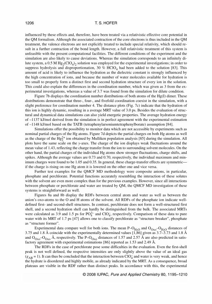
influenced by these effects and, therefore, have been treated via a relativistic effective core potential inthe QM formalism. Although the associated contraction of the core electrons is thus included in the QMtreatment, the valence electrons are not explicitly treated to include special relativity, which should re-sult in a further contraction of the bond length. However, a full relativistic treatment of this system isunfeasible with the present computational facilities. The different conditions of the experiment and thesimulation are also likely to cause deviations. Whereas the simulation corresponds to an infinitely di-lute system, a 0.5 M Hg2(ClO4)2 solution was employed for the experimental investigations; in order tosuppress hydrolysis and disproportionation, 30 % HClO4 had been added to the solution [83]. Thisamount of acid is likely to influence the hydration as the dielectric constant is strongly influenced bythe high concentration of ions, and because the number of water molecules available for hydration istoo small to properly form a distinct first and second hydration structure of every ion in the solution.This could also explain the differences in the coordination number, which was given as 3 from the ex-perimental investigations, whereas a value of 3.7 was found from the simulation for dilute condition.

Figure 7b displays the coordination number distributions of both atoms of the Hg(I) dimer. Thesedistributions demonstrate that three-, four-, and fivefold coordination coexist in the simulation, with aslight preference for coordination number 4. The distance plots (Fig. 7c) indicate that the hydration ofthis ion is highly dynamic, resulting in a average MRT value of 3.0 ps. Besides the evaluation of struc-tural and dynamical data simulations can also yield energetic properties. The average hydration energyof –1137 kJ/mol derived from the simulation is in perfect agreement with the experimental estimationof –1148 kJ/mol based on the TATB (tetraphenylarsoniumtetraphenylborate) assumption [84].

Simulations offer the possibility to monitor data which are not accessible by experiments such asnominal partial charges of the Hg atoms. Figure 7d depicts the partial charges on both Hg atoms as wellas the charge of the Hg2

2+ ion obtained by Mulliken population analysis [85] during the simulation. Allplots have the same scale on the y-axes. The charge of the ion displays weak fluctuations around themean value of 1.43, reflecting the charge transfer from the ion to surrounding solvent molecules. On theother hand, the partial charges of the individual Hg atoms show stronger fluctuations, charge shifts, andspikes. Although the average values are 0.73 and 0.70, respectively, the individual maximum and min-imum charges were found to be 1.05 and 0.35. In general, these charge-transfer effects are symmetric—if the charge is rising on one Hg atom it is lowered on the other one and vice versa.

Further test examples for the QMCF MD methodology were composite anions, in particular,phosphate and perchlorate. Potential functions accurately resembling the interaction of these soluteswith the solvent are even more complex than for the previous examples. However, since all interactionsbetween phosphate or perchlorate and water are treated by QM, the QMCF MD investigation of thesesystems is straightforward as well.

Figures 8a and 8b display the RDFs between central atom and water as well as between theanion’s oxo-atoms to the O and H atoms of the solvent. All RDFs of the phosphate ion indicate well-defined first- and second-shell structures. In contrast, perchlorate does not form a well-structured firstshell, and a second hydration shell can hardly be distinguished from the bulk. The associated MRTswere calculated as 3.9 and 1.5 ps for PO4

3– and ClO4–, respectively. Comparison of these data to pure

water with its MRT of 1.7 ps [47] allows one to classify perchlorate as “structure breaker”, phosphateas “structure former”.

Experimental data compare well for both ions. The mean P–OH2O and OOxo–OH2O distances of3.75 and 1.8 Å coincide with the experimentally determined values [1,86] given as 3.7–3.73 and 1.8 Åand OOxo–OOxo Å, respectively. The P–OOxo distances of 1.57 and 2.57 Å are also predicted in satis-factory agreement with experimental estimations [86] reported as 1.53 and 2.49 Å.

The RDFs in the case of perchlorate pose some difficulties in the evaluation. Even the first-shellpeak is not well defined, the respective intensities are only slightly above the value of an ideal gas(gAB = 1). It can thus be concluded that the interaction between ClO4

– and water is very weak, and hencethe hydrate is disordered and highly mobile, as already indicated by the MRT. As a consequence, broadplateaus are visible in the RDF rather than distinct peaks. In accordance with this, the experimental

T. S. HOFER


1206

Cl–OH2Odistance, given as 3.6–4.0 Å [1,87,88], has a standard deviation of ~0.3 Å. A distinct maxi-mum is difficult to determine from the RDF of the simulation—only an interval can be given rangingfrom 3.9 to 4.2 Å. However, the excellent agreement of the Cl–OOxo distance of 1.45 Å with experi-mental results reporting 1.43–1.45 Å [87,88] indicates that the simulation reflects the complex situationof this very labile hydrate quite well.

Further analysis of these systems focusing on vibrational as well as energetic properties will giveadditional data to characterize these complex ionic species. Data obtained from a recent QMCF MDsimulation of SO4

2– in aqueous solution are in good agreement with data obtained from LAXS experi-ments [89]. Further investigations focusing on the hydration energy and vibrational motions of thisoxoanion [90] have demonstrated that this novel simulation method allows a thorough study of a vari-ety of properties in a general, accurate, and straightforward way.

CONCLUSION

The QM/MM MD methodology proves to be a versatile technique for the study of solvated species.Especially in cases where high exchange rates and/or a varying preference for ligands result in differ-ent simultaneously present solvate species with varying coordination numbers and bond lengths, thuscomplicating experimental investigations, simulation methods serve as a useful tool to investigate sol-vation processes. The simulation data support the construction of fitting models and can, therefore,prove essential for an unambiguous evaluation of experimental measurements.

Difficulties in the simulation of systems of low symmetry or of composite compounds have beenovercome by the QMCF MD formalism, which is capable of treating all solute–solvent interactions onthe basis of quantum mechanics and a fluctuating charge field. The examples presented here make usconfident that present ab initio simulation methods exhibit a level of accuracy to reliably predict prop-erties of solvated species. As computational hard- and software resources are constantly improving, thecontinuous progress in accuracy as well as in applicability of these simulation techniques will be main-tained if not accelerated.

ACKNOWLEDGMENTS

Support of this work by the Austrian Science Foundation (FWF) and the Hypo Tirol Bank is gratefullyacknowledged.



Fig. 8 RDFs of (a) the center atoms and (b) the oxo–atoms to the hydrogen (solid line) and oxygen atoms (dashedline) of water obtained from QMCF MD simulations of PO4

3– and ClO4–, respectively. (c) Snapshot of phosphate in

aqueous solution.

REFERENCES AND NOTES

1. H. Ohtaki, T. Radnai. Chem. Rev. 93, 1157 (1993). 2. G. W. Neilson, J. E. Enderby. The Coordination of Metal Aquaions, Vol. 34, pp. 195–218,

Academic Press, Orlando (1989). 3. L. Helm, A. E. Merbach. Chem. Rev. 105, 1923 (2005). 4. M. P. Allen, D. J. Tildesley. Computer Simulation of Liquids, Oxford Science Publications,

Oxford (1990). 5. McQuarrie. Statistical Mechanics, Harper & Row, New York (1976). 6. R. P. H. Gasser, W. G. Richards. An Introduction to Statistical Thermodynamics, World Scientific,

Singapore (1995). 7. A. J. Stone. The Theory of Intermolecular Forces, Oxford University Press, Oxford (1995). 8. A. R. Leach. Molecular Modelling, 2nd ed., Prentice-Hall, Essex (2001).9. F. Jensen. Introduction to Computational Chemistry, John Wiley, Chichester (1999).

10. C. J. Cramer. Essentials of Computational Chemistry, John Wiley, West Sussex (2002). 11. H. Ohtaki. Chem. Monthly 132, 1237 (2001). 12. G. W. Neilson, A. K. Adya. Ann. Rep. Chem., Sect. C 93, 101 (1996). 13. G. W. Neilson, P. E. Mason, S. Ramos, D. Sullivan. Philos. Trans. R. Soc. London, Ser. A 359,

1575 (2001). 14. L. Helm, A. E. Merbach. Coord. Chem. Rev. 187, 151 (1999). 15. A. J. Lock, S. Woutersen, H. J. Bakker. Femtochemistry and Femtobiology, World Scientific,

Singapore (2001). 16. P. Wernet, D. Nordlund, U. Bergmann, M. Cavalleri, M. Odelius, H. Ogasawara, L. A. Näslund,

T. K. Hirsch, L. Ojamäe, P. Glatzel, L. G. M. Pettersson, A. Nilsson. Science 304, 955 (2004). 17. J. B. R. Bucher, J. Stauber. Chem. Phys. Lett. 306, 57 (1999). 18. D. Frenkel, B. Smit. Understanding Molecular Simulation, Academic Press, San Diego (2002). 19. R. J. Sadus. Molecular Simulation of Fluids, Elsevier Science, Amsterdam (1999). 20. C. J. Cramer, D. G. Truhlar. Chem. Rev. 99, 2161(1999). 21. F. P. Rotzinger. Chem. Rev. 105, 2003 (2005). 22. N. Metropolis, A. W. Rosenbluth, M. N. Rosenbluth, A. H. Teller, E. Teller. J. Chem. Phys. 21,

1087 (1953). 23. D. A. Pearlman, D. A. Case, J. W. Caldwell, W. Ross, T. Cheatham, S. DeBolt, D. Ferguson,

G. Seibel, P. Kollman. Comp. Phys. Commun. 91, 1 (1995). 24. A. D. MacKerell, B. Brooks, C. L. Brooks (III), L. Nilsson, B. Roux, Y. Won, M. Karplus.

“CHARMM: The Energy Function and Its Parameterization with an Overview of the Program”,in The Encyclopedia of Computational Chemistry, John Wiley, Chichester (1998).

25. B. R. Brooks, R. E. Bruccoleri, B. D. Olafson, D. J. States, S. Swaminathan, M. Karplus. J. Comp.Chem. 4, 187 (1983).

26. E. Schrödinger. Ann. Phys. 79, 361 (1926). 27. M. Nooijen. Phys. Rev. Lett. 84, 2108 (2000). 28. H. Nakatsuji. J. Chem. Phys. 113, 2949 (2000). 29. L. Thøgersen, J. Olsen, D. Yeager, P. Jørgensen, P. Salek, T. Helgaker. J. Chem. Phys. 121, 16

(2004). 30. R. Car, M. Parinello. Phys. Rev. Lett. 55, 2471 (1985). 31. J. P. Perdew, K. Burke, M. Ernzerhof. Phys. Rev. Lett. 77, 3865 (1996). 32. J. P. Perdew, K. Burke, M. Ernzerhof. Phys. Rev. Lett. 78, 1396 (1997). 33. A. D. Becke. Phys. Rev. A 38, 3098 (1988). 34. A. Pasquarello, I. Petri, P. S. Salmon, O. Parisel, R. Car, É. Tóth, D. H. Powell, H. E. Fischer,

L. Helm, A. Merbach. Science 291, 856 (2001). 35. I. Bakó, J. Hutter, G. Pálinkás. J. Chem. Phys. 117, 9838 (2002).

T. S. HOFER


1208

36. W. Kutzelnigg. Density Functional Theory (DFT) and ab initio Quantum Chemistry (AIQC):Story of a Difficult Partnership, G. Maroulis, T. Simos (Eds.), p. 23, International SciencePublishers (VSP), Leiden (2006).

37. D. J. Harris, J. P. Brodholt, D. M. Sherman. J. Phys. Chem. B 107, 9056 (2003). 38. R. J. Bartlett, I. V. Schweigert, V. F. Lotrich. J. Mol. Struct. (Theochem) 764, 33 (2006). 39. R. J. Bartlett, V. F. Lotrich, I. V. Schweigert. J. Chem. Phys. 123, 062205 (2005). 40. A. D. Becke. J. Chem. Phys. 98, 5648 (1993). 41. H. M. Senn, W. Thiel. Curr. Opin. Chem. Biol. 11, 182 (2007). 42. H. Lin, D. G. Truhlar. Theor. Chem. Acc. 117, 185 (2007). 43. A. Warshel, M. Levitt. J. Mol. Biol. 103, 227 (1976). 44. M. J. Field, P. A. Bash, M. Karplus. J. Comput. Chem. 11, 700 (1990). 45. J. Gao. J. Am. Chem. Soc. 115, 2930 (1993). 46. D. Bakowies, W. Thiel. J. Phys. Chem. 100, 10580 (1996). 47. D. Xenides, B. R. Randolf, B. M. Rode. J. Chem. Phys. 122, 4506 (2005). 48. D. Xenides, B. R. Randolf, B. M. Rode. J. Mol. Liq. 123, 61 (2006). 49. C. F. Schwenk, A. Tongraar, B. M. Rode. J. Mol. Liq. 110, 105 (2004). 50. B. M. Rode, C. F. Schwenk, T. S. Hofer, B. R. Randolf. Coord. Chem. Rev. 249, 2993 (2005). 51. C. F. Schwenk, B. M. Rode. J. Am. Chem. Soc. 126, 12786 (2004). 52. B. M. Rode, T. S. Hofer, B. R. Randolf, C. F. Schwenk, D. Xenides, V. Vchirawongkwin. Theor.

Chem. Acc. 115, 77 (2006). 53. A. Laio, J. VandeVondele, U. Rothlisberger. J. Chem. Phys. 116, 6941 (2002). 54. E. Voloshina, N. Gaston, B. Paulus. J. Chem. Phys. 126, 134115 (2007). 55. C. F. Schwenk, T. S. Hofer, B. M. Rode. J. Phys. Chem. A 108, 1509 (2004). 56. P. R. Smirnov, V. N. Trostin. Russ. J. Phys. Chem. 69, 1097 (1995). 57. T. S. Hofer, H. T. Tran, C. F. Schwenk, B. M. Rode. J. Comput. Chem. 25, 211 (2004). 58. A. Tongraar, B. M. Rode. Chem. Phys. Lett. 409, 304 (2005). 59. C. F. Schwenk, H. H. Loeffler, B. M. Rode. Chem. Phys. Lett. 349, 99 (2001). 60. T. S. Hofer, B. R. Randolf, B. M. Rode. J. Phys. Chem. B 110, 20409 (2006). 61. T. S. Hofer, B. M. Rode, B. R. Randolf. Chem. Phys. 312, 81 (2005). 62. R. Armunanto, C. F. Schwenk, B. M. Rode. J. Phys. Chem. A 107, 3132 (2003). 63. R. Armunanto, C. F. Schwenk, H. T. Tran, B. M. Rode. J. Am. Chem. Soc. 126, 2582 (2004). 64. C. Kritayakornupong, K. Plankensteiner, B. M. Rode. Chem. Phys. Lett. 371, 438 (2003). 65. T. S. Hofer, A. B. Pribil, B. R. Randolf, B. M. Rode. J. Am. Chem. Soc. 127, 14231 (2005). 66. M. Q. Fatmi, T. S. Hofer, B. R. Randolf, B. M. Rode. J. Chem. Phys. 123, 4514 (2005). 67. T. S. Hofer, B. M. Rode. J. Chem. Phys. 121, 6406 (2004). 68. C. F. Schwenk, B. M. Rode. ChemPhysChem 4, 931 (2003). 69. C. F. Schwenk, B. M. Rode. J. Chem. Phys. 119, 9523 (2003). 70. I. Persson, P. Persson, M. Sandström, A.-S. Ullström. J. Chem. Soc., Dalton Trans. 7, 1256

(2002). 71. C. Kritayakornupong, K. Plankensteiner, B. M. Rode. ChemPhysChem 5, 1499 (2004). 72. C. F. Schwenk, T. S. Hofer, B. R. Randolf, B. M. Rode. Phys. Chem. Chem. Phys. 7, 1669 (2005). 73. M. Q. Fatmi, T. S. Hofer, B. R. Randolf, B. M. Rode. Phys. Chem. Chem. Phys. 8, 1675 (2006). 74. M. Q. Fatmi, T. S. Hofer, B. R. Randolf, B. M. Rode. J. Phys. Chem. B 111, 151 (2007). 75. D. H. Powell, L. Helm, A. E. Merbach. J. Chem. Phys. 95, 9258 (1991). 76. P. S. Salmon, M. C. Bellissent-Funel, G. J. Herdman. J. Phys. Condens. Matter 2, 4297 (1990). 77. A. Tongraar, K. Sagarik, B. M. Rode. Phys. Chem. Chem. Phys. 4, 628 (2002). 78. R. Armunanto, C. F. Schwenk, B. R. Randolf, B. M. Rode. Chem. Phys. Lett. 388, 395 (2004). 79. R. Armunanto, C. F. Schwenk, B. M. Rode. J. Am. Chem. Soc. 126, 9934 (2004). 80. T. S. Hofer, B. R. Randolf, S. A. A. Shah, B. M. Rode, I. Persson. Chem. Phys. Lett. 445, 193

(2007).



81. J. Purans, B. Fourest, C. Cannes, V. Sladkov, F. David, L. Venault, M. Lecomte. J. Phys. Chem.B 109, 11074 (2005).

82. J. M. Martinez, F. Torrico, R. R. Pappalardo, E. S. Marcos. J. Phys. Chem. A 108, 15851 (2004). 83. J. Rosdahl, I. Persson, L. Kloo, K. Stahl. Inorg. Chem. A 357, 2624 (2004). 84. M. Yizhak. Ion Properties, Marcel Dekker, New York (1997). 85. R. S. Mulliken. J. Chem. Phys. 23, 1833 (1955). 86. P. Mason, J. Cruickshank, G. Neilson, P. Buchanan. Phys. Chem. Chem. Phys. 5, 4690 (2003).87. G. W. Neilson, D. Schiöoberg, W. Luck. Chem. Phys. Lett. 122, 475 (1985). 88. G. Johansson, H. Wakita. Inorg. Chem. 24, 3047 (1985). 89. V. Vchirawongkwin, I. Persson, B. M. Rode. J. Phys. Chem. B 111, 4150 (2007). 90. V. Vchirawongkwin, B. M. Rode. J. Phys. Chem. 10, 1016 (2007).

T. S. HOFER


1210

capabilities of chemical simulation methods in the

Documents