signal detection of adverse drug reaction using the
TRANSCRIPT

University of South FloridaScholar Commons
Graduate Theses and Dissertations Graduate School
March 2018
Signal Detection of Adverse Drug Reaction usingthe Adverse Event Reporting System: LiteratureReview and Novel MethodsMinh H. PhamUniversity of South Florida, [email protected]
Follow this and additional works at: http://scholarcommons.usf.edu/etd
Part of the Bioinformatics Commons, Medicinal Chemistry and Pharmaceutics Commons, andthe Statistics and Probability Commons
This Thesis is brought to you for free and open access by the Graduate School at Scholar Commons. It has been accepted for inclusion in GraduateTheses and Dissertations by an authorized administrator of Scholar Commons. For more information, please contact [email protected].
Scholar Commons CitationPham, Minh H., "Signal Detection of Adverse Drug Reaction using the Adverse Event Reporting System: Literature Review and NovelMethods" (2018). Graduate Theses and Dissertations.http://scholarcommons.usf.edu/etd/7218

Signal Detection of Adverse Drug Reaction using the Adverse Event Reporting System:
Literature Review and Novel Methods
by
Minh H. Pham
A thesis submitted in partial fulfillment of the requirements
for the degree of Master of Arts in Statistics
Department of Mathematics and Statistics
College of Arts and Sciences
University of South Florida
Major Professor: Kandethody M. Ramachandran, Ph.D.
Feng Cheng, Ph.D.
Chris P. Tsokos, Ph.D.
Date of Approval:
March 27, 2018
Keywords: Association Study, Pharmacovigilance,
Statistical Algorithms, Big Data, Data Mining.
Copyright © 2018, Minh H. Pham

DEDICATION
To my parents: for their unconditional love, support, and sacrifices. You taught me well
the value of discipline and hard work.
To my sister: for your encouragement and support. You have always encouraged me to
pursue what I love.
To Won Yi and Malko Cajuste: for your guidance and care. You have made me a more
well-rounded person.

ACKNOWLEDGMENTS
I would like to gratefully acknowledge grant 7AZ23 from the Ed and Ethel Moore
Alzheimer's Disease Research Program, Florida Department of Health. The grant allowed us to
combine all the FAERS data submissions and store in a local database at the University of South
Florida. The database was used extensively in this thesis.
I owe my deepest gratitude to my thesis advisor Dr. Kandethody Ramachandran for
accepting to chair my thesis. Thank you for advising my work, opening my mind, and
challenging me to do better.
I would like to thank Dr. Feng Cheng for suggesting the problem and serving on my
thesis committee. Thank you forgiving insights and directions to my thesis work.
I would like to thank Dr. Chris Tsokos for serving on my thesis committee. Thank you
for your time and valuable feedback on my thesis work.

i
TABLE OF CONTENTS
LIST OF TABLES ....................................................................................................................................... iii
LIST OF FIGURES ..................................................................................................................................... iv
ABSTRACT .................................................................................................................................................. v
CHAPTER I: INTRODUCTION AND PROBLEM STATEMENT ............................................................ 1
CHAPTER 2: LITERATURE REVIEW ...................................................................................................... 4
2.1 Association Rules .......................................................................................................................... 4
2.2 Collective Strength ........................................................................................................................ 8
2.3 Proportional Reporting Ratio & Reporting Odds Ratio .............................................................. 10
2.4 Dependence Rules (Chi-Squared Test) ....................................................................................... 13
2.5 Gamma-Poisson Shrinkage Model (aka Empirical Bayes Geometric Mean) ............................. 16
2.6 Bayesian Confidence Propagation Neural Network (aka Information Component) ................... 19
2.7 Logistic Regression ..................................................................................................................... 23
2.8 Regression - Adjusted Gamma-Poisson Shrinkage Model ......................................................... 25
CHAPTER 3: THE NOVEL METHODS ................................................................................................... 28
3.1 Tree-Based Methods ................................................................................................................... 29
3.1.1 Decision Tree ...................................................................................................................... 29
3.1.2 Random Forests................................................................................................................... 32
3.1.3 Variable Importance ............................................................................................................ 33
3.2 Monte Carlo Logic Regression ................................................................................................... 34

ii
3.2.1 Logic Regression................................................................................................................. 35
3.2.2 Monte Carlo Logic Regression ........................................................................................... 38
CHAPTER 4: COMPARISON STUDY ..................................................................................................... 40
4.1 The Gold Standard for Testing .................................................................................................... 40
4.2 The FAERS Database ................................................................................................................. 41
4.3 Computational details ................................................................................................................. 43
4.4 Results of Performance Testing .................................................................................................. 43
CHAPTER 5: CONCLUSION AND DISCUSSION OF FUTURE WORK .............................................. 47
REFERENCES ........................................................................................................................................... 50
Appendix A: OMOP Gold Standard List .................................................................................................... 58
Appendix B: RGPS Code ............................................................................................................................ 69

iii
LIST OF TABLES
Table 1: Contingency Table for PRR and ROR............................................................................ 11
Table 2: Three-way contingency table for Chi-squared test ......................................................... 14
Table 3: Contingency Table for Information Component ............................................................ 20
Table 4: Merging and Transforming Drug Table and Reaction Table ......................................... 41
Table 5: Areas Under Curve ......................................................................................................... 44
Table 6: Computing Time ............................................................................................................. 45

iv
LIST OF FIGURES
Figure 1:Neural Network by bate et al. ......................................................................................... 20
Figure 2: An example of Decision Tree ........................................................................................ 30
Figure 3: An example of Logic Tree ............................................................................................. 35
Figure 4: Demonstration of the six moves to modify Logic Tree................................................. 37
Figure 5: ROC curve of 7 different methods ................................................................................ 44

v
ABSTRACT
One of the objectives of the U.S. Food and Drug Administration is to protect the public
health through post-marketing drug safety surveillance, also known as Pharmacovigilance. An
inexpensive and efficient method to inspect post-marketing drug safety is to use data mining
algorithms on electronic health records to discover associations between drugs and adverse
events.
The purpose of this study is two-fold. First, we review the methods and algorithms
proposed in the literature for identifying association drug interactions to an adverse event and
discuss their advantages and drawbacks. Second, we attempt to adapt some novel methods that
have been used in comparable problems such as the genome-wide association studies and the
market-basket problems. Most of the common methods in the drug-adverse event problem have
univariate structure and thus are vulnerable to give false positive when certain drugs are usually
co-prescribed. Therefore, we will study applicability of multivariate methods in the literature
such as Logistic Regression and Regression-adjusted Gamma-Poisson Shrinkage Model for the
association studies. We also adopted Random Forest and Monte Carlo Logic Regression from the
genome-wide association study to our problem because of their ability to detect inherent
interactions. We have built a computer program for the Regression-adjusted Gamma Poisson
Shrinkage model, which was proposed by DuMouchel in 2013 but has not been made available

vi
in any public software package. A comparison study between popular methods and the proposed
new methods is presented in this study.

1
CHAPTER I: INTRODUCTION AND PROBLEM STATEMENT
In order to monitor adverse events of drugs that have been approved for marketing, the
US Food and Drug Administration (FDA) has organized the FDA Adverse Event Reporting
System (FAERS) since 1968 [1]. FAERS is a rich data source for the study and identification of
adverse reactions to regulated drugs in the US. This database contains over 2 million voluntary
reports of pharmaceutical products in the world and increases by more than 300,000 reports each
year [2, 3]. For the past four decades, the FAERS database have played a major role in signaling
known and unknown adverse events that are associated with single or interacted drugs. If a
potential safety concern is discovered through FAERS, the FDA then performs other evaluations
and might take regulatory actions to protect the public health, such as restricting the signaled
drug, updating information labels, or removing the product from the market [1].
Despite its critical role in Pharmacovigilance, the FAERS database has limitations and
presents challenging problems to data scientists in designing statistical processes and algorithm
to detect safety signals. First, safety signals, even correct and significant signals, do not always
present cause-effect relationship between drugs and adverse events because according to the
FDA’s requirements for data collection, the relationship between reported adverse event and
drug are not necessarily proven to be causal-effect. Second, since patients and their service
providers may independently report the same adverse events to the database, duplicated reports

2
are possible and is in fact a well-known problem for the FAERS database [1]. In order to tackle
the duplicated report problem, researchers usually take into account the case versions and
discrepancies between FAERS and the FDA’s legacy data [34]. Finally, the gigantic and rapidly
increasing size of FAERS (more than 1 million records of prescribed drugs added every quarter
[1]) creates challenges in computational statistics, resolving event and drug dictionary problems
and data miscoding [18].
The study of drug-adverse event association problem is a fairly new problem in the
literature. The first systematic studies that addressed this specific problem were carried out in the
early 2000s [2 – 4, 11, 12]. However, the literature has progressed quickly because of its
similarities with other problems such as the market basket problem [6-10] and the genome-wide
association problem [4, 5]. In the market basket problem, researchers attempt to identify patterns
of the type “A customer purchasing item A is likely to purchase item B”. In the genome-wide
association problem, we find associations between genomic patterns and diseases or traits.
The drug-adverse event problem could be mathematically stated as follows. Given a set of drugs
𝑋1, 𝑋2, … , 𝑋𝑝 and a set of adverse events 𝑌1, 𝑌2, … , 𝑌𝑞, the objective is to find the set of drugs that
associates with a specific adverse event 𝑌ℎ, 1 ≤ ℎ ≤ 𝑞. Mathematically speaking, we would like
to generate all sets that contain one or more drugs and one adverse event, (𝑋𝑖, 𝑋𝑗, … 𝑋𝑘, 𝑌ℎ), 1 ≤
𝑖, 𝑗, 𝑘 ≤ 𝑝 , that have significant association measures between event 𝑌ℎ and drug(s) 𝑋𝑖, 𝑋𝑗, … , 𝑋𝑘.
Various measures of association have been proposed by researchers in the literature such as
Proportional Reporting Ratio [11], Reporting Odds Ratio [13], Relative Risk [20], and
Information Component [32]. If a set has only one X, the drug is called associated with event 𝑌ℎ.
Two or more X’s indicate drug interactions that created the adverse event.

3
The remainder of this thesis is organized in 4 chapters. Chapter 2 presents the notable
statistical tests and algorithms and the survey of research related to the problem being addressed.
In Chapter 3, we discuss the Random Forest algorithm and Monte Carlo Logic Regression that
we introduced for drug association studies because they have interesting properties that might
tackle the challenges. In Chapter 4, we perform a comparison study between the commonly used
data mining methods and the novel methods using the Observational Medical Outcomes
Partnership’s Gold Standard as a testing bed. The concluding remarks and the suggested future
work are presented in Chapter 5.

4
CHAPTER 2: LITERATURE REVIEW
The following notations are used to describe the methodologies. Suppose our data has n
rows corresponding to n cases. Variables 𝑋1, 𝑋2, … , 𝑋𝑝 indicate use of drugs (1 means used, 0
means not used). Variables 𝑌1, 𝑌2, … , 𝑌𝑞 indicate presence of q adverse events. Variables
𝑍1, 𝑍2, … , 𝑍𝑟 contain demographic information, such as age and gender. The data’s dimension is
n*(p + q + r).
For the remainder of this thesis, we use 𝑋𝑖,𝑗 to denote the ith column and jth row entry of
matrix X. Therefore, 𝑋𝑖,𝑙, 𝑌𝑗,𝑙, 𝑍𝑘,𝑙 denote the values of each variable at the lth case in the data
where 𝑋𝑖,𝑙 and 𝑌𝑗,𝑙 take value of 0 or 1 for all i, j, l. For instance, 𝑋3,10 = 1 means that the patient
in the 10th row took drug 𝑋3, 𝑌5,20 = 1 means that the patient in the 20th row observed adverse
event 𝑌5.
2.1 Association Rules
Association Rules was introduced for the market basket problem by Agrawal et al. in
1993, [6].
Let 𝑁𝑖 = ∑ 𝑋𝑖𝑙𝑛𝑙=1 be the count of rows that observe the use of drug 𝑋𝑖 (1 ≤ i ≤ p and 1 ≤ l ≤ n
is the index for cases), 𝑁𝑖𝑗 = ∑ 𝑋𝑖𝑙𝑌𝑗𝑙𝑛𝑙=1 be count of rows that observe both drug 𝑋𝑖 = 1 and
adverse event 𝑌𝑗 = 1 (1 ≤ j ≤ q). Association Rules uses confidence as a measure of

5
interestingness, which is the probability of observing adverse event 𝑌𝑗 given 𝑋𝑖 is present
𝑃(𝑌𝑗 = 1|𝑋𝑖 = 1) =𝑁𝑖𝑗
𝑁𝑖. The method is conducted through 2 steps:
• Support is the proportion of data that observe both 𝑋𝑖 = 1 and 𝑌𝑗 = 1. This proportion
is 𝑁𝑖𝑗
𝑛. Select all sets of 𝑋𝑖 and 𝑌𝑗 that have support higher than an arbitrary threshold:
𝑁𝑖𝑗
𝑛≥ 𝑆0
• From the sets found in the previous step, identify the sets that have confidence higher
than an arbitrary threshold: 𝑃(𝑌𝑗 = 1|𝑋𝑖 = 1) =𝑁𝑖𝑗
𝑁𝑖≥ 𝐶0
There is no definitive way to determine the thresholds 𝑆0 and 𝐶0. The choice of thresholds is
subject to the context of the data set and how interesting the associations are [33].
Finding association between three or more items is done in similar fashion, where support is
the proportion of records that observe all of 𝑋𝑖, 𝑋𝑖′, and 𝑌𝑗 in the data and confidence is the
probability of observing event 𝑌𝑗 given both 𝑋𝑖and 𝑋𝑖′ is present. More specifically, the two steps
Association Rules are now:
• Select all sets of 𝑋𝑖 and 𝑌𝑗 that have support, which is the percentage of observing all of
𝑋𝑖, 𝑋𝑖′, and 𝑌𝑗 in the data 𝑁𝑖𝑖′𝑗
𝑛 where 𝑁𝑖𝑖′𝑗 = ∑ 𝑋𝑖𝑙𝑋𝑖′𝑙𝑌𝑗𝑙
𝑛𝑙=1 , higher than an arbitrary
threshold: 𝑁𝑖𝑖′𝑗
𝑛≥ 𝑆0
• From the sets found in the previous step, identify the sets that have confidence higher
than an arbitrary threshold: 𝑃(𝑌𝑗 = 1|𝑋𝑖 = 1 & 𝑋𝑖′ = 1) =𝑁𝑖𝑖′𝑗
𝑁𝑖≥ 𝐶0

6
In real-world practice, it is common that the number of drugs p and the number of events q
are so large that we cannot consider all combinations of drug-adverse event because generating
and evaluating all combinations is computationally intensive. Only considering combinations of
one drug and one event, the total number of combinations we need to consider is 𝑝 × 𝑞, which
can be immensely big if the dataset has thousands of drugs and events. Algorithms such as
Apriori [7] or FP-growth [8] are designed to finish the first step efficiently by reducing the
number of item sets that we must consider. Apriori algorithm does this by eliminating an item set
if any of its subset does not have enough support. FP-tree compresses data into a tree structure
where frequent item sets lay on top of the tree and can easily be found.
Advantages of Association Rules:
Being one of the first methods to be proposed in the association study literature,
Association Rule is intuitive and easy to implement. This method is also computationally less
intensive than the later ones because all computational operations include only summing and
logical comparisons.
Drawbacks of Association Rules:
The simple operation does not make statistical soundness in many cases because it does
not adjust for the popularity of individual drug or correlation. Brin & Motwani [9] gives the
following example to illustrate its weakness. Consider drug 𝑋1 and adverse event 𝑌2 with the
total number of records n = 100, 𝑁1 = 25 records have 𝑋1 = 1, 𝑁2 = 90 records have 𝑌2 = 1, 𝑁12
= 20 records have 𝑋1 = 1 𝑎𝑛𝑑 𝑌2 = 1, and 5 records have 𝑋1 = 0 and 𝑌2 = 0.
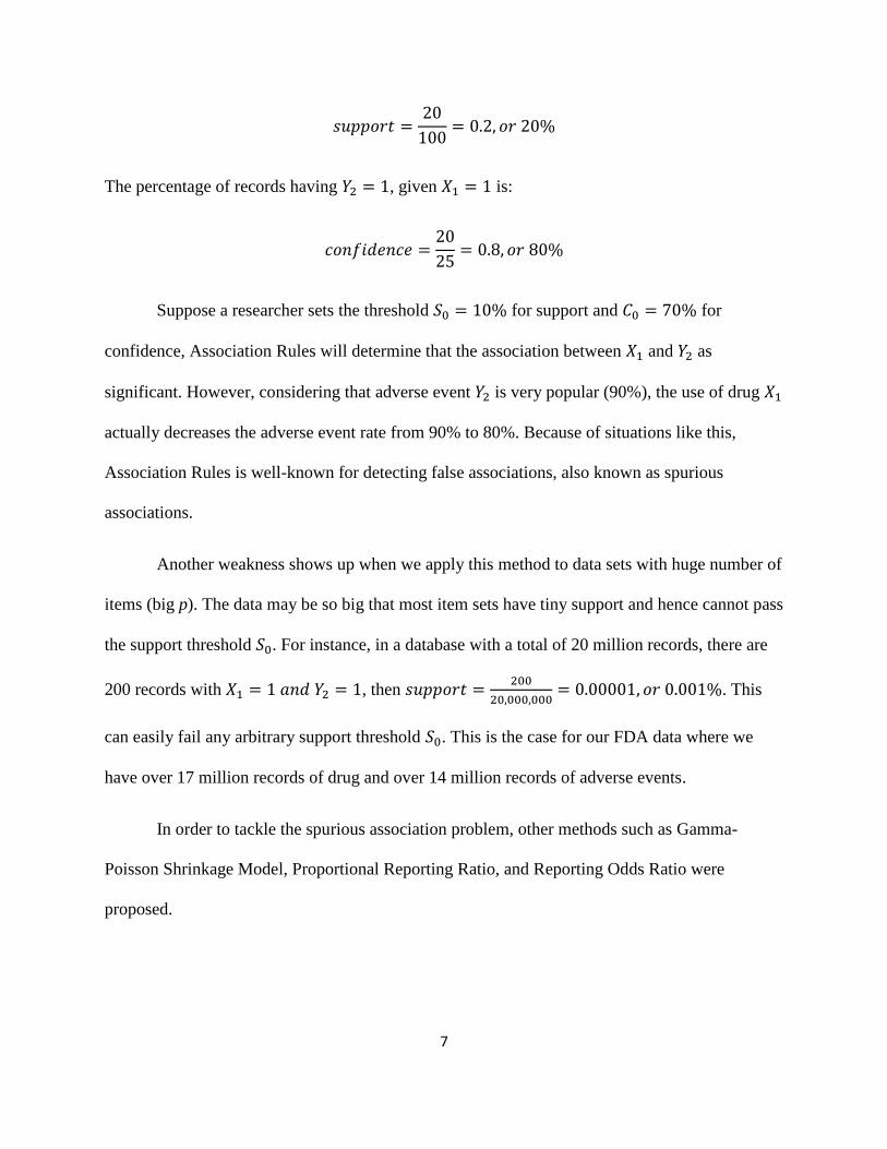
The percentage of records having 𝑋1 = 1 𝑎𝑛𝑑 𝑌2 = 1 is:
7
𝑠𝑢𝑝𝑝𝑜𝑟𝑡 =20
100= 0.2, 𝑜𝑟 20%
The percentage of records having 𝑌2 = 1, given 𝑋1 = 1 is:
𝑐𝑜𝑛𝑓𝑖𝑑𝑒𝑛𝑐𝑒 =20
25= 0.8, 𝑜𝑟 80%
Suppose a researcher sets the threshold 𝑆0 = 10% for support and 𝐶0 = 70% for
confidence, Association Rules will determine that the association between 𝑋1 and 𝑌2 as
significant. However, considering that adverse event 𝑌2 is very popular (90%), the use of drug 𝑋1
actually decreases the adverse event rate from 90% to 80%. Because of situations like this,
Association Rules is well-known for detecting false associations, also known as spurious
associations.
Another weakness shows up when we apply this method to data sets with huge number of
items (big p). The data may be so big that most item sets have tiny support and hence cannot pass
the support threshold 𝑆0. For instance, in a database with a total of 20 million records, there are
200 records with 𝑋1 = 1 𝑎𝑛𝑑 𝑌2 = 1, then 𝑠𝑢𝑝𝑝𝑜𝑟𝑡 =200
20,000,000= 0.00001, 𝑜𝑟 0.001%. This
can easily fail any arbitrary support threshold 𝑆0. This is the case for our FDA data where we
have over 17 million records of drug and over 14 million records of adverse events.
In order to tackle the spurious association problem, other methods such as Gamma-
Poisson Shrinkage Model, Proportional Reporting Ratio, and Reporting Odds Ratio were
proposed.

8
2.2 Collective Strength
As an attempt to solve the spurious association problem of Association Rules that was
discussed in section 2.1, Aggarwal and Yu proposed a new measure of association, Collective
Strength [10].
Let I be an item set of drug(s) and an adverse events, 𝐼 = (𝑋𝑖, 𝑋𝑗 , … 𝑋𝑘, 𝑌ℎ), 1 ≤ 𝑖, 𝑗, 𝑘 ≤
𝑝. Aggarwal and Yu defined violation v(I) of an item set I as the sets containing some but not all
items of I. Suppose we are evaluating drug 𝑋𝑖 and adverse event 𝑌𝑗, 𝐼 = (𝑋𝑖, 𝑌𝑗) is the event of
using drug 𝑋𝑖 and observing adverse event 𝑌𝑗. The violation 𝑣(𝐼) is the event of observing either
𝑋1 = 1 or 𝑌1 = 1, but not both: 𝑣(𝐼) = (𝑋𝑖 = 1 𝑎𝑛𝑑 𝑌𝑗 = 0) 𝑜𝑟 (𝑋𝑖 = 0 𝑎𝑛𝑑 𝑌𝑗 = 1).
We can then estimate the probability of violation event from the data: 𝑃(𝑣(𝐼)) =
∑ 𝐼(𝑋𝑖𝑙=1 𝑎𝑛𝑑 𝑌𝑗𝑙=0) 𝑜𝑟 (𝑋𝑖𝑙=0 𝑎𝑛𝑑 𝑌𝑗𝑙=1)
𝑛𝑙=1
𝑛.
Collective Strength is then defined as: 𝐶(𝐼) =1−𝑃(𝑣(𝐼))
1−𝐸(𝑃(𝑣(𝐼)))∗
𝐸(𝑃(𝑣(𝐼)))
𝑃(𝑣(𝐼)), 0 ≤ 𝐶(𝐼) ≤ ∞,
where 𝐸(𝑃(𝑣(𝐼))) is calculated by assuming the independence of items and using raw
probabilities of individual items. In our notations, 𝐸(𝑃(𝑣(𝐼))) = 1 − 𝑃(𝑋𝑖 = 1)𝑃(𝑌𝑗 = 1) −
𝑃(𝑋𝑖 = 0)𝑃(𝑌𝑗 = 0), where 𝑃(𝑋𝑖 = 1), 𝑃(𝑌𝑗 = 1), 𝑃(𝑋𝑖 = 0), 𝑃(𝑌𝑗 = 0) are estimated from
the data as follows.
𝑃(𝑋𝑖 = 1) =∑ 𝑋𝑖𝑙
𝑛𝑙=1
𝑛
𝑃(𝑌𝑖 = 1) =∑ 𝑌𝑗𝑙
𝑛𝑙=1
𝑛
𝑃(𝑋𝑖 = 0) = 1 − 𝑃(𝑋𝑖 = 1)

9
𝑃(𝑌𝑖 = 0) = 1 − 𝑃(𝑌𝑖 = 1)
Collective Strength 𝐶(𝐼) can take any value from 0 to infinity. A value of 0 indicates perfectly
negative correlation between 𝑋𝑖 and 𝑌𝑗, i.e. 𝑌𝑗 = 0 when 𝑋𝑖 = 1 and vice versa. 𝐶(𝐼) = 1
indicates no association between 𝑋𝑖 and 𝑌𝑗 . The more 𝐶(𝐼) exceeds 1, the stronger the
association between 𝑋𝑖 and 𝑌𝑗.
Advantages of Collective Strength:
The authors proved that Collective Strength does not suffer from detecting false positive
because it considers the presence/absence of individual items. In addition, it has nice
computational properties that allow the setup of algorithms that works as efficiently as
Association Rules for large number of items.
Drawbacks of Collective Strength:
The convenient computational properties come with the price of loss of interpretability as
a measure of association, since the formula of Collective Strength does not suggest any useful
meaning. Compared to other measures of association described later such as Relative Reporting
Rate, Proportional Reporting Rate, or Reporting Odds Ratio, Collective Strength is a lot less
intuitive.
To illustrate this weakness, let’s consider an item set I = {𝑋1, 𝑌1}, where the probability
of observing each item is 0.1: 𝑃(𝑋1 = 1) = 𝑃(𝑌1 = 1) = 0.1. Under independence assumption
(no association), the expectation of observing both 𝑋1 and 𝑌1 is 0.12 = 0.01. Suppose we
observe from the data that the probability of observing both items is 0.05.

10
Using the formulae above, we can obtain the Collective Strength value 𝐶(𝐼) = 1.09. This is
somewhat close to 1, which shows the weakness of the method because we cannot interpret how
strong an association with C(I) = 1.09 is. However, if we compare the expected and observed
frequency of I, we can see that observed frequency is 5 times higher than expectation
(0.05/0.01), which should indicate a strong association. This measurement of 5 times higher than
expectation is called Relative Report Rate and is utilized in the Gamma-Poisson Shrinkage
model below.
All methods described later in this thesis are based on statistical development and their
measures of association are more meaningful and statistically grounded than Collective Strength
and thus will be better alternatives than Collective Strength in evaluating associations.
2.3 Proportional Reporting Ratio & Reporting Odds Ratio
Proportional Reporting Ratio (PRR) and Reporting Odds Ratio (ROR) are both
meaningful and popular measures of association [11-13] that can test the association between
one drug 𝑋𝑖 and one event 𝑌𝑗. To calculate both PRR and ROR, we first calculate the four
counting values:
𝑎 = ∑ 𝐼𝑋𝑖,𝑙=1 𝑎𝑛𝑑 𝑌𝑗,𝑙=1
𝑛
𝑙=1
𝑏 = ∑ 𝐼𝑋𝑖,𝑙=0 𝑎𝑛𝑑 𝑌𝑗,𝑙=1
𝑛
𝑙=1
𝑐 = ∑ 𝐼𝑋𝑖,𝑙=1 𝑎𝑛𝑑 𝑌𝑗,𝑙=0
𝑛
𝑙=1

11
𝑑 = ∑ 𝐼𝑋𝑖,𝑙=0 𝑎𝑛𝑑 𝑌𝑗,𝑙=0
𝑛
𝑙=1
Simply put, a is the count of cases where both 𝑋𝑖 and 𝑌𝑗 are observed, b is the count of
cases where 𝑋𝑖 is not observed but 𝑌𝑗 is, c is the count of cases where 𝑋𝑖 is observed but 𝑌𝑗 is not,
and d is the count of cases where neither 𝑋𝑖 nor 𝑌𝑗 is observed. We can construct the following
contingency table:
Table 1: Contingency Table for PRR and ROR
Drug 𝑋𝑖 Other drugs
Effect 𝑌𝑗 a b
Other effects c d
PRR and ROR can then be calculated as:
𝑃𝑅𝑅 =𝑎/(𝑎 + 𝑐)
𝑏/(𝑏 + 𝑑)
𝑅𝑂𝑅 =𝑎/𝑐
𝑏/𝑑
PRR is the ratio between having side effect using drug A over having side effect using all
other drugs. ROR measures the ratio between the odds ratio of side effect using drug A and the
odds ratio of side effect using all other drugs. They both approach to 1 if there is no association
between Drug A and Effect B and are bigger than 1 if the association is significant. Each
measure was proven superior in certain scenarios [13].

12
We can construct confidence intervals for PRR and ROR as follows. PRR and ROR have
skew distributions, since they are lower bounded by zero but have no upper bound. However, the
logarithm of PRR and ROR can take any value and are approximately Normal distributed when
a, b, c, d are sufficiently large [43]. Therefore, the confidence interval of PRR can be calculated
as (𝑃𝑅𝑅
exp(𝑧𝛼𝑠), 𝑃𝑅𝑅 ∗ exp (𝑧𝛼𝑠)) where 𝑧𝛼 is the critical value from the Standard Normal
Distribution and 𝑠 = √1
𝑎+
1
𝑐−
1
𝑎+𝑏−
1
𝑐+𝑑. The confidence interval for ROR is calculated as
𝑒log(𝑅𝑂𝑅) ±(𝑧𝛼∗𝑠) where 𝑠 = √1
𝑎+
1
𝑏+
1
𝑐+
1
𝑑. These calculations are subject to the assumption of
Normality. A pair of drug and adverse event is determined to have significant association if the
lower bound of the confidence interval of PRR or ROR is larger than 1.
Advantages of PRR and ROR:
These two measures are simple to implement and both have meaningful interpretations.
PRR and ROR measure how often an adverse event is reported for individuals taking a drug,
compared to the frequency that the same adverse event is reported for patients taking other drugs.
Drawbacks of PRR and ROR:
There are three major issues if ROR and PRR are applied to our problem. First, since
PRR and ROR compare the frequencies of an adverse event between taking a particular drug and
taking other drugs, they use data of other drugs as benchmarks. If many drugs in the data are
associated with the adverse event, comparison between the benchmarks and a drug that has true
positive but not as frequent association will return a weak signal. Second, these methods require
specification of drug 𝑋𝑖 and side effect 𝑌𝑗. In a large database such as FAERS, there are

13
thousands of drugs and side effects and hence testing every pair of drug and effect is
computationally inefficient. Finally, these methods cannot test more than one drug at a time and
hence cannot be used to detect drug-drug interactions to create adverse events.
2.4 Dependence Rules (Chi-Squared Test)
Silverstein et al. also attempted to find an alternative to Association Rules using Chi-
squared Test of Independence [14].
Using the Contingency table in Table 1, we calculate the expected count of each cell
under the null hypothesis of independence as:
𝐸11 =(𝑎 + 𝑏)(𝑎 + 𝑐)
𝑛
𝐸12 =(𝑎 + 𝑏)(𝑏 + 𝑑)
𝑛
𝐸21 =(𝑎 + 𝑐)(𝑐 + 𝑑)
𝑛
𝐸11 =(𝑏 + 𝑑)(𝑐 + 𝑑)
𝑛
The Chi-squared test statistic is:
𝜒2 = ∑ ∑(𝑂𝑖𝑗 − 𝐸𝑖𝑗)
2
𝑗=1
2
𝑖=1
where 𝑂𝑖𝑗 is the observed count of cell (i, j) (a, b, c, or d). The test statistic has 3 degrees of
freedom.

14
Chi-squared test is robust and is solidly grounded in statistical theory, but it suffers from
two major weaknesses. First, it is sensitive to samples of size if any expected frequency is less
than 5. Second, regular Chi-squared test of independence can only be applied to two variables. In
our drug-effect problem, it can be used to test for independence between one drug and one
association, but is useless with testing for drug interaction where we have more than 2 drugs and
an effect.
To overcome the second problem, Silverstein et al. provides a framework for Chi-squared
test of independence for more than 3 variables. The process is very similar to the 2-variable Chi-
squared test. Suppose we have two drugs 𝑋1, 𝑋2 and an adverse event 𝑌3 as defined in the
introduction. We would like to test the null hypothesis that they are pairwise independent as
follows.
First, we construct a three-way contingency table:
Table 2: Three-way contingency table for Chi-squared test
𝑋1 = 1 𝑋1 = 0
𝑌3 = 1
𝑋2 = 1 𝑂1,1,1 𝑂0,1,1
𝑋2 = 0 𝑂1,0,1 𝑁0,0,1
𝑋1 = 1 𝑋1 = 0
𝑌3 = 0
𝑋2 = 1 𝑂1,1,0 𝑂0,1,0
𝑋2 = 0 𝑂1,0,0 𝑂0,0,0

15
where 𝑂𝑖,𝑗,𝑘 = ∑ 𝐼𝑋1,𝑙=𝑖 𝑎𝑛𝑑 𝑋2,𝑙=𝑗 𝑎𝑛𝑑 𝑌3,𝑙=𝑘𝑛𝑙=1 is the observed count of each cell. The expected
counts under the null hypothesis is:
𝐸𝑖,𝑗,𝑘 =∑ (𝐼𝑋1,𝑙=𝑖 )
𝑛𝑙=1
𝑛∗
∑ (𝐼𝑋2,𝑙=𝑗 )𝑛𝑙=1
𝑛∗
∑ (𝐼𝑌3,𝑙=𝑘 )𝑛𝑙=1
𝑛∗ 𝑛
=∑ (𝐼𝑋1,𝑙=𝑖 )
𝑛𝑙=1 ∗ ∑ (𝐼𝑋2,𝑙=𝑗 )
𝑛𝑙=1 ∗ ∑ (𝐼𝑌3,𝑙=𝑘 )
𝑛𝑙=1
𝑛2
Then the Chi-squared statistic is 𝜒2 = ∑(𝑂𝑖,𝑗,𝑘 − 𝐸𝑖,𝑗,𝑘)2
/𝐸𝑖,𝑗,𝑘 with 4 degree of freedom.
There is a flaw if we want to apply this approach to our drug-effect problem. The Chi-
Squared test also considers the dependency between 𝑋1 and 𝑋2 that we are not interested. We are
only interested in the correlation of (𝑋1& 𝑌3), (𝑋2& 𝑌3), or (𝑋1& 𝑋2 & 𝑌3).
One way to overcome this problem is to combine 𝑋1, 𝑋2 into a new variable with 4
categories, namely (00,01,10,11), and then apply the 2-variable Chi-squared test. Nevertheless,
the test will not tell us whether 𝑋1, 𝑋2, or combination of 𝑋1𝑋2 is accountable for significant side
effect.
The problem with small sample remains unsolved for Chi-squared test. Chi-squared test,
PRR, and ROR are all better alternatives than Association Rules and Collective Strength in
evaluating drug-event association because they are built upon statistical theories. However, they
all have drawbacks when it comes to testing small samples. This problem is well known for Chi-
squared test [15, 16]. PRR and ROR’s confidence interval are constructed using standard normal
distribution [17], which is also problematic for small samples. The two methods Gamma-Poisson
Shrinkage Model and Information Component both attempt to overcome this issue by assuming
parametric distributions on their measures of association and finding Bayesian posterior

16
distributions. The Bayesian methods have more complicated calculations, but they are both more
conservative when sample size gets smaller.
2.5 Gamma-Poisson Shrinkage Model (aka Empirical Bayes Geometric
Mean)
The Gamma-Poisson Shrinkage Model (GPS) was first developed to detect associations
of international calls at AT&T, but the FDA adopted the method to their own database and found
about 40,000 drug-event signals [23].
We use the same notations. Let 𝑁𝑖 = ∑ 𝑋𝑖𝑙𝑛𝑙=1 be the number of occurrence of drug 𝑋𝑖 (1 ≤ i ≤ p
and 1 ≤ l ≤ n is the index for cases), 𝑁𝑖𝑗 = ∑ 𝑋𝑖𝑙𝑌𝑗𝑙𝑛𝑙=1 be the number of occurrence of both 𝑋𝑖
and 𝑌𝑗 (1 ≤ j ≤ q).
A measurement of association that makes logical soundness is Relative Reporting Rate:
𝑅𝑅𝑖𝑗 =𝑁𝑖𝑗
𝐸(𝑁𝑖𝑗)=
𝑁𝑖𝑗
𝐸𝑖𝑗
where 𝐸𝑖𝑗 = 𝑃(𝑋𝑖 = 1) ∗ 𝑃(𝑌𝑗 = 1) ∗ 𝑁 = 𝑁𝑖 ∗ 𝑁𝑗/𝑁 is the expected count of observing both 𝑋𝑖
and 𝑌𝑗 under the null hypothesis that 𝑋𝑖 and 𝑌𝑗 are independent.
If 𝑅𝑅𝑖𝑗 ≫ 1, which means the count of (𝑋𝑖 = 1 𝑎𝑛𝑑 𝑌𝑗 = 1) is much larger than its
expectation under the independence hypothesis, an association between 𝑋𝑖 and 𝑋𝑗 is likely.
DuMouchel developed the Gamma-Poisson Shrinkage Model (GPS) to test for the significance
of this measurement with the Bayesian approach [19, 20]. The test is carried out as follow:

17
Assume that 𝑁𝑖𝑗~𝑃𝑜𝑖𝑠𝑠𝑜𝑛(𝜆𝑖𝑗 ∗ 𝐸𝑖𝑗), 1 ≤ 𝑖 ≤ 𝑝, 1 ≤ 𝑗 ≤ 𝑞 where all the 𝜆𝑖𝑗′𝑠 is drawn
from a common prior distribution, which is assumed to be a mixture of two Gamma
distributions. The parameters of the prior distribution is estimated from the raw data of 𝜆𝑖𝑗 =𝑁𝑖𝑗
𝐸𝑖𝑗.
We are interested in calculating 𝑃(𝜆𝑖𝑗 > 1), since 𝜆𝑖𝑗 > 1 means the adverse event happens
more frequent expected and thus signals drug-adverse event association. The author chose a
mixture of 2 Gamma distributions as prior to exploit the conjugate prior property so that the
posterior distribution has a closed form. He first used a single Gamma Distribution as prior to
utilize the Gamma-Poisson conjugate property, but then needed a more flexible prior distribution
because he estimated the prior distribution from a whole data set. Therefore, a Gamma mixture
was chosen to preserve the availability of closed-form solution and to increase the goodness-of-
fit. According to the conjugate property, the unconditional distribution of each 𝑁𝑖𝑗 is a mixture of
2 negative binomial distributions [22]. The probability density function of the parameter 𝜆𝑖𝑗 is
given as:
𝜋(𝜆; 𝛼1, 𝛽1, 𝛼2, 𝛽2, 𝑝) = 𝑝𝑔(𝜆; 𝛼1, 𝛽1) + (1 − 𝑝)𝑔(𝜆; 𝛼2, 𝛽2), 𝛼1, 𝛽1, 𝛼2, 𝛽2 > 0, 0 ≤ 𝑝 ≤ 1
where 𝑔(𝜆; 𝛼1, 𝛽1) and 𝑔(𝜆; 𝛼2, 𝛽2) are the probability density functions of the Gamma
Distribution with shape parameters 𝛼1, 𝛼2 and scale parameters 𝛽1, 𝛽2, and 𝑝 is the weight of the
first distribution. The probability density function of the Gamma Distribution [21] is given by:
𝑓(𝑥, 𝛼, 𝛽) =𝛽𝛼
Γ(𝛼)𝑥𝛼−1𝑒−𝛽𝑥
Let 𝜃 = (𝛼1, 𝛽1, 𝛼2, 𝛽2, 𝑝)′. To estimate how much 𝜆𝑖𝑗 exceeds 1 from the data, the author
applied the Empirical Bayesian approach with the following steps:

18
• The unconditional distribution of each 𝑁𝑖𝑗 is a mixture of 2 negative binomial
distributions with parameter 𝜃. We can calculate Maximum Likelihood estimates of 𝜃
based on data of 𝑁𝑖𝑗′𝑠 and 𝐸𝑖𝑗’s as follows.
The Log-Likelihood function is:
𝑙(𝜆; 𝛼1, 𝛽1, 𝛼2, 𝛽2, 𝑝) = ∑ ln (𝑝𝛽1
𝛼1
Γ(𝛼1)𝑥𝑖
𝛼1−1𝑒−𝛽1𝑥𝑖 + (1 − 𝑝)
𝛽2𝛼2
Γ(𝛼2)𝑥𝑖
𝛼2−1𝑒−𝛽2𝑥𝑖)
𝑛
𝑖=1
We would like to find 𝜃 = (𝛼1, 𝛽1, 𝛼2, 𝛽2, 𝑝)′ such that 𝜕𝑙(𝜆;𝜃)
𝜕𝜃= 0. Obviously, a close-
form solution is not available. Therefore, we need to use Newton-type numerical methods
to estimate the solution of 𝜕𝑙(𝜆;𝜃)
𝜕𝜃= 0 [57, 58].
• For each 𝑁𝑖𝑗, we compute the posterior distribution of 𝜆𝑖𝑗 as 𝑃𝑜𝑖(𝑁𝑖𝑗|𝜆𝑖𝑗 ∗ 𝐸𝑖𝑗)𝜋(𝜆𝑖𝑗|𝜃)/
∫ 𝑃𝑜𝑖(𝑁𝑖𝑗|𝜆𝑖𝑗 ∗ 𝐸𝑖𝑗)𝜋(𝜆𝑖𝑗|𝜃) 𝑑𝜆, where 𝑃𝑜𝑖(𝑋|𝜆) is the Poisson probability mass
function with mean 𝜆.
• For each cell (i, j), obtain the 5th percentile of the posterior distribution 𝜆0.05. In other
words, 𝜆0.05 is the lower 95% confidence bound of 𝜆. We can then make a decision rule
that, if 𝜆0.05 > 1, the association of (i, j) item is significant. Since 𝜆 > 1 means a
significant association, this decision rule will put the probability of false positive, which
is 𝑃(𝜆 > 1|𝜆0.05 > 1), lower than 0.05.
The model is named Shrinkage because 𝜆0.05 gets smaller if 𝑁𝑖𝑗 is smaller, thus makes the
test more conservative when observed size is small. The prior distribution is not pre-specified but
estimated from the data. Therefore, this method follows the Empirical Bayes approach.
Advantages of GPS:

19
This method fixes all weaknesses of Association Rules, Collective Strength, and Chi-
squared test: it has good interpretability of the measurement of association, statistical soundness,
and applicability to small samples. Since the method uses the Empirical Bayes approach by
estimating the prior distribution from the data, it provides inferences that are conditional on the
data and are not reliant on asymptotic approximation. Therefore, we can expect this method to
outperform the frequentist methods such as ROR, PRR, and Chi-squared when small samples are
considered.
Drawbacks of GPS:
There are three main problems with this method. First, it cannot easily take into account
the effect of demographic variables in our data (age and gender). In order to do this, the
DuMouchel et al. had to stratify the data based on these covariates and repeat the same process
[7]. This is computationally intensive especially when we have many stratums. Second, this
method is not applicable to test more than one drug at once, which means that we cannot test for
drug-drug interactions to create adverse event. Finally, the choice of mixture of Gamma
Distribution as the prior distribution should be used with caution since the Bayesian approach
might produce posterior distribution that are heavily influenced by the prior distribution [24].
2.6 Bayesian Confidence Propagation Neural Network (aka Information
Component)
In 1996, Lansner and Holst studied the training and inference of Neural Network using
the Bayesian training rule, which they called Bayesian Confidence Propagation Neural Network

20
(BCPNN) [35]. When Bate et al. [36] applied the method to the drug-effect problem, he used a
simple neural network with one input layer as drugs and one output layers as adverse events:
Figure 1:Neural Network by bate et al.
The expectation of the weight between input 𝑥𝑖 and output 𝑞𝑖 was found to be:
𝑤 = log2(𝑃(𝑞𝑖, 𝑥𝑖)
𝑃(𝑞𝑖)𝑃(𝑥𝑖))
which is called the Information Component (IC), and is also the log of Relative Reporting Rate
in GPS method. As Bate et al. developed the method for the drug association problem, he moved
away from the neural network and focused more on the estimation of IC. Therefore, even though
the method inherits the name “Bayesian Confidence Propagation Neural Network”, it is in fact
univariate and we do not actually interpret the results with the neural network.
Noren et al. described the Baysian estimates of IC as follows. We would like to estimate
the distributions of 𝑃(𝑞𝑖, 𝑥𝑖), 𝑃(𝑞𝑖), 𝑃(𝑥𝑖). Using the same set up as in PRR and ROR, we
consider the contingency table that is calculated from the data:
Table 3: Contingency Table for Information Component

21
Drug 𝑋𝑖 Other Drugs
Event 𝑌𝑗 𝑛11 𝑛10
Other events 𝑛01 𝑛00
where
𝑛11 = ∑ 𝐼𝑌𝑗,𝑙=1 𝑎𝑛𝑑 𝑋𝑖,𝑙=1
𝑛
𝑙=1
𝑛10 = ∑ 𝐼𝑌𝑗,𝑙=1 𝑎𝑛𝑑 𝑋𝑖,𝑙=0
𝑛
𝑙=1
𝑛01 = ∑ 𝐼𝑌𝑗,𝑙=0 𝑎𝑛𝑑 𝑋𝑖,𝑙=1
𝑛
𝑙=1
𝑛00 = ∑ 𝐼𝑌𝑗,𝑙=0 𝑎𝑛𝑑 𝑋𝑖,𝑙=0
𝑛
𝑙=1
𝑛.. = 𝑛11 + 𝑛10 + 𝑛01 + 𝑛00 = 𝑛
We assume that (𝑛11, 𝑛10, 𝑛01, 𝑛00) follows the Multinomial distribution with Probability
Mass Function:
𝑃(𝑛11, 𝑛10, 𝑛01, 𝑛00|𝑛, 𝑝11, 𝑝10, 𝑝01, 𝑝00) =𝑛!
𝑛11! 𝑛10! 𝑛01! 𝑛00!𝑝11
𝑛11𝑝10𝑛10𝑝01
𝑛01𝑝00𝑛00
where 𝑛 = 𝑛11 + 𝑛10 + 𝑛01 + 𝑛00 and (𝑝11, 𝑝10, 𝑝01, 𝑝00) are parameters. These parameters are
assumed to follow the Dirichlet distribution Dir(𝛼11, 𝛼10, 𝛼01, 𝛼00) as the prior distribution. The
probability density function of the prior distribution is:

22
𝑓(𝑝11, 𝑝10, 𝑝01, 𝑝00|𝛼11, 𝛼10, 𝛼01, 𝛼00) =1
Β(𝛼11, 𝛼10, 𝛼01, 𝛼00)𝑝11
𝛼11𝑝10𝛼10𝑝01
𝛼01𝑝00𝛼00
where Β(𝛼11, 𝛼10, 𝛼01, 𝛼00) is the the multivariate Beta function. The prior parameters are
calculated according to the assumption of independence between the drug and the adverse event:
𝛼11 = 𝑞1.𝑞.1𝛼..
𝛼10 = 𝑞1.𝑞.0𝛼..
𝛼01 = 𝑞10𝑞.1𝛼..
𝛼00 = 𝑞0.𝑞.0𝛼..
where
𝛼.. =0.5
𝑞1.𝑞.1
𝑞1. =𝑛1. + 0.5
𝑛.. + 1
𝑞0. =𝑛0. + 0.5
𝑛.. + 1
𝑞.1 =𝑛.1 + 0.5
𝑛.. + 1
𝑞.0 =𝑛.0 + 0.5
𝑛.. + 1
The conjugate prior property makes the posterior distribution Dirichlet with parameters
(𝛾11, 𝛾10, 𝛾01, 𝛾00) where 𝛾𝑖𝑗 = 𝛼𝑖𝑗 + 𝑛𝑖𝑗 , 𝑖, 𝑗 ∈ {0,1} .

23
Knowing the posterior distribution for (𝑝11, 𝑝10, 𝑝01, 𝑝00), we can calculate the
expectation of IC as:
𝐸(𝐼𝐶) = log2(𝐸(𝑝11)
𝐸(𝑝1.)𝐸(𝑝.1))
Obviously, the closed form of distribution of IC is unknown, we need to estimate the lower 95%
confidence bound by Monte Carlo Simulation or Normal Approximation.
If the lower 95% bound is larger than 0, a signal is determined.
The Bayesian approaches, GPS and IC, were proven to have better performance than
PRR, ROR, and Chi-squared with higher area under the Receiver Operating Characteristic
(ROC) curve [28]. With modern computer’s strength, performing complex Bayesian calculation
is not too intensive and therefore, GPS and IC should be a superior choice over PRR, ROR, or
Chi-squared.
2.7 Logistic Regression
PRR, ROR, GPS, and BCPNN are called Disproportionality methods. They all have two
drawbacks. First, they cannot easily consider demographic variables such as age and gender.
Second, they are vulnerable to raise false positive for co-prescribed drugs. For example, drug A
and drug B are often prescribed together but only drug A causes a side effect. Disproportionality
methods, even the Bayesian ones, will likely find drug B associated with the side effect because
the two drugs are not considered simultaneously. Logistic Regression (LR) was first applied to
this type of problem by DuMouchel (2004) [25]. An advantage of Logistic Regression over all

24
the previous methods is that it considers all variables at once and hence is less vulnerable to the
co-prescribed drugs situation.
The logic is straight forward: we consider each adverse event 𝑌𝑗 (1 ≤ 𝑗 ≤ 𝑞) as a binary
response variable and all drugs 𝑋1, 𝑋2, … , 𝑋𝑝 as explanatory variables. The logistic regression has
the form:
𝑙𝑜𝑔𝑖𝑡 (𝑃(𝑌𝑗 = 1)) = log (𝑃(𝑌𝑗 = 1)
1 − 𝑃(𝑌𝑗 = 1)) = ∑𝛽𝑖𝑋𝑖
We can also add demographic information 𝑍𝑖 as covariates:
𝑙𝑜𝑔𝑖𝑡(𝑝(𝑌ℎ)) = log (𝑃(𝑌𝑗 = 1)
1 − 𝑃(𝑌𝑗 = 1)) = ∑𝛽𝑖𝑋𝑖 + ∑𝛼𝑖𝑍𝑖
We are interested in the significance of 𝛽𝑖’s in this regression using the usual t-test.
Interestingly, a recent study that compared the methods using FDA data shows that Logistic
Regression family performs better than GPS and generally has higher specificity at a given level
of sensitivity [27]
To investigate drug-drug interaction, we just need to add the interaction terms to the
model:
𝑙𝑜𝑔𝑖𝑡(𝑝(𝐴)) = ∑𝛽𝑖𝐷𝑖 + ∑𝛼𝑖𝑋𝑖 + ∑𝛾𝑖𝐷𝑖𝐷𝑗
However, this will increase the number of parameters quickly. 1,000 drugs will yield 500,000
interaction terms, which can easily exceed the amount of data to fit. An alternative is to include
only the drug combinations that are observed in the data more than an arbitrary threshold. For

25
example, we may only include in the model the pairs of drugs that are co-prescribed more than 5
times in the data.
Another drawback of logistic regression is that it requires a large amount of data to obtain
a stable model. A recent study shows that a 20:1 ratio between numbers of observations and
parameters are needed [26]. Nevertheless, this is not our issue since we are currently dealing
with rather large FAERS database.
2.8 Regression - Adjusted Gamma-Poisson Shrinkage Model
DuMouchel’s GPS method was found to perform worse than Logistic Regression
[27].However, the use of t-test in Logistic Regression is vulnerable to small samples, which was
one of the reasons why GPS was introduced [19]. In 2012, DuMouchel combined GPS and LR
into a hybrid method that has strengths of both [28]. The main idea is to replace the t-test of
coefficient significance in LR by GPS instead of the t-test. First we select a subset of p drugs to
fit the Logistic Regression model. Suppose the subset of predicting drugs is 𝑆 ⊂ {1, 2, … , 𝑝}. The
Logistic Regression model is:
𝑙𝑜𝑔𝑖𝑡 (𝑃(𝑌𝑗 = 1)) = ∑ 𝛽𝑖𝑋𝑖
𝑖⊂𝑆
In the publication, DuMouchel selects the predicting drugs based on their event rates. We
can rewrite this equation to include all drugs 𝑋𝑖, 1 ≤ 𝑖 ≤ 𝑝, but set 𝛽𝑖 = 0 if 𝑖 ⊄ 𝑆:
𝑙𝑜𝑔𝑖𝑡 (𝑃(𝑌𝑗 = 1)) = ∑ 𝛽𝑖𝑋𝑖
𝑝
𝑖=1
, 𝑤ℎ𝑒𝑟𝑒 𝛽𝑖 = 0 𝑖𝑓 𝑖 ⊄ 𝑆

26
Unlike the regular Logistic Regression, we do not use the t-test for significance of 𝛽𝑖’s as
the final decision. Instead, DuMouchel proposed to calculate the expected count of observing
both 𝑋𝑘, 1 ≤ 𝑘 ≤ 𝑝, and 𝑌𝑗 under the null hypothesis that drug 𝑋𝑘 has no effect on event 𝑌𝑗 to be
used for the rest of the GPS process. The null hypothesis is equivalent to 𝛽𝑘 = 0. Therefore, the
expected probability of event 𝑌𝑗 = 1 is calculated as:
𝐸(𝑙𝑜𝑔𝑖𝑡 (𝑃(𝑌𝑗 = 1))) = ∑ 𝛽𝑖𝑋𝑖
𝑝
𝑖=1
− 𝛽𝑘𝑋𝑘
therefore,
𝐸 (𝑃(𝑌𝑗 = 1)) = 1/(1 + ∑ 𝛽𝑖𝑋𝑖
𝑝
𝑖=1
− 𝛽𝑘𝑋𝑘)
We apply this formula to each row of the data (each patient in the data) to calculate each
of their expected count of observing event 𝑌𝑗 . Then, the expected count of event 𝑌𝑗 under the null
hypothesis 𝛽𝑘 = 0 is the sum of 𝐸 (𝑃(𝑌𝑗 = 1)) across all data records (again, rows are indexed
with 1 ≤ 𝑙 ≤ 𝑛):
𝐸𝑘𝑗 = ∑(1
1 + ∑ 𝛽𝑖𝑋𝑖𝑙𝑝𝑖=1 − 𝛽𝑘𝑋𝑘𝑙
)
𝑛
𝑙=1
This process is repeated for each of the drugs 𝑋𝑘, 1 ≤ 𝑘 ≤ 𝑝. As a result, we get an array
of expected counts 𝐸𝑘𝑗 of observing both drug 𝑋𝑘, 1 ≤ 𝑘 ≤ 𝑝, and adverse event 𝑌𝑗 , 1 ≤ 𝑗 ≤ 𝑞.
In the original GPS method, this is calculated based on raw data: 𝐸𝑘𝑗 = 𝑃(𝑋𝑘 = 1) ∗
𝑃(𝑌𝑗 = 1)/𝑁 = 𝑁𝑘 ∗ 𝑁𝑗/𝑁.

27
GPS method is then continued as in section 2.6 with this new expected count 𝐸𝑘𝑗 =
∑ (1
1+∑ 𝛽𝑖𝑋𝑖𝑙𝑝𝑖=1
−𝛽𝑘𝑋𝑘𝑙)𝑛
𝑙=1
Regression-adjusted GPS was proven in the same study to have better performance than
both LR and GPS [28]. This is intuitive because it combines the sample size-sensitive Bayesian
method and the multivariate method of calculating expected count.
Since RGPS is not available in any public software package, we attempted to write the
program according to DuMouchel’s description. We made a slight adjustment to the algorithm
however. We do not select the predicting variables based on their event rates but using a forward
step-wise algorithm with Akaike information criterion [55].

28
CHAPTER 3: THE NOVEL METHODS
All the methods discussed in Chapter 2 suffer from a common problem. They do not
automatically evaluate interactions between drugs unless we clearly state the specific interactions
in the model (only for Chi-squared Test and Logistic Regression). Specifying interactions might
be arduous or even impossible when the number of drugs p and the number of adverse events q
get large. Therefore, we attempt to apply two algorithms, Random Forests and Monte Carlo
Logic Regression, to this drug association problem. These two algorithms can detect interactions
between input variables along with the main effects without specifying the interactions. They
were both successfully applied in genome-wide association studies to detect both the main
effects and interactions [37 - 42].
For both methods, we consider a specific adverse event 𝑌𝑗 , 1 ≤ 𝑗 ≤ 𝑞 (output variable)
and all drugs in the data 𝑋1, 𝑋2, … , 𝑋𝑝 (input variables). Both methods attempt to predict the
value of 𝑌𝑗 using the given values of 𝑋1, 𝑋2, … , 𝑋𝑝 and evaluate the significance of each of the
input variables and their interactions in the process.

29
3.1 Tree-Based Methods
Random Forests is a non-parametric method for regression and classification and requires
no assumption about the data [44, 45]. To describe Random Forests, we first need to introduce
Decision Trees, which is a simpler method for regression and classification.
3.1.1 Decision Tree
Decision Tree consists of many levels of decision nodes, each splits the one of the input
variables into two categories. Therefore, a Decision Tree partitions the input variables’ domain,
and the bottom branches of a Decision Tree show the predicted values for each partition. Figure
2 shows an example of a Decision Tree using notations from our problem. The ending boxes to
the far right of the tree, labeled either 0 or 1, indicates the best prediction value of 𝑌𝑗 for that
partition. For example, the top branch of the tree means that when 𝑋1 = 1 𝑎𝑛𝑑 𝑋2 = 1 then the
best prediction for 𝑌𝑗 is 1.

30
Figure 2: An example of Decision Tree
We now discuss the process of building an optimized Decision Tree. The goal is to divide
the predictor space, which is the set of all possible values of 𝑋1, 𝑋2, … , 𝑋𝑝, into J distinct and
non-overlapping regions 𝑅1, 𝑅2, … , 𝑅𝐽 with 𝑛1, 𝑛2, … , 𝑛𝐽 observations respectively. For each
region 𝑅𝑚, 1 ≤ 𝑚 ≤ 𝐽, the predicted value is the most common class in that region. The
classification error rate in region 𝑅𝑚 is the proportion of observations not equal to predictions:
1 − �̂�𝑚 = 1 −1
𝑛𝑚max ( ∑ 𝐼(𝑌𝑗 = 0)
𝑋1,𝑋2,…,𝑋𝑝∈ 𝑅𝑚
, ∑ 𝐼(𝑌𝑗 = 1)
𝑋1,𝑋2,…,𝑋𝑝∈ 𝑅𝑚
)
Then the classification error rate for the whole tree is: 1 − �̂� =1
𝑛∑ 𝑛𝑚(1 − �̂�𝑚)𝐽
𝑚=1
Gini Index is another measure of region purity. Since our classification problem only has
two classes 0 and 1, the Gini Index formula [45] is reduced to:

31
𝐺 = 2�̂�𝑚(1 − �̂�𝑚)
The goal is to construct a decision tree with the highest measure of purity. Breiman [46]
described the process of finding the best decision tree using a greedy algorithm as follows.
• Starting with all the data, for each input variable 𝑋𝑖, 1 ≤ 𝑖 ≤ 𝑝, we split the input space
into two half-planes: 𝑅1(𝑖) = {𝑋|𝑋𝑗 = 0} 𝑎𝑛𝑑 𝑅2(𝑖) = {𝑋|𝑋𝑗 = 1}. Then we calculate
the misclassification rate 1 − �̂�(𝑖) =1
𝑛∑ 𝑛𝑚(1 − �̂�𝑚)2
𝑚=1 .
• Select the input variable 𝑋𝑖 that has the lowest misclassification rate 1 − �̂�(𝑖).
• Having found the best splitting variable, we partition the data into two sub-regions 𝑅1
and 𝑅2.
• Repeat this process on each sub-region until the misclassification rate stops decreasing.
How many times should we split the data, or how large should we grow the tree? A common
strategy is to grow a very large tree, called tree 𝑇0, until the sample sizes 𝑛𝑗 , 1 ≤ 𝑗 ≤ 𝐽 reach a
pre-determined number (usually 5). Then this large tree is simplified by cost-complexity pruning
as follows.
We define a subtree 𝑇 of 𝑇0 to be any tree that can be obtained by removing a number of
𝑇0’s non-terminal nodes. Let |𝑇| denote the number of terminal nodes in 𝑇. The false
classification rate in region 𝑅𝑚 of tree 𝑇 is:
1 − �̂�𝑚(𝑇) =1
𝑛𝑚max ( ∑ 𝐼(𝑌𝑗 = 0)
𝑋1,𝑋2,…,𝑋𝑝∈ 𝑅𝑚
, ∑ 𝐼(𝑌𝑗 = 1)
𝑋1,𝑋2,…,𝑋𝑝∈ 𝑅𝑚
)
The cost-complexity criterion is define by

32
𝐶𝛼(𝑇) = ∑ 𝑛𝑚(1 − �̂�𝑚(𝑇))
|𝑇|
𝑚=1
+ 𝛼|𝑇|
where 𝛼 is the penalizing parameter for the tree size, which can be determined by cross-
validation [45]. For each value of 𝛼, there is only a finite number of sub-trees 𝑇 and we find the
sub-tree that produces the lowest 𝐶𝛼(𝑇).
3.1.2 Random Forests
Decision Tree suffers from high variance, which means that a slight change in the data
can yield a significantly different tree and prediction. Random Forests is a popular way to reduce
variance and increase prediction power [46]. Random Forests makes two improvements on
Decision Tree:
First, we bootstrap the data by taking repeated B samples from the training data set,
generally by repeatedly sampling 2/3 of the data. We then train Decision Tree on each of the B
bootstrapped samples and average all the predictions. Suppose we have B Decision Trees 𝑇𝑏 , 1 ≤
𝑏 ≤ 𝐵 corresponding to B bootstrapped samples, the prediction for an input vector 𝑥 is:
𝑇(𝑥) =1
𝐵∑ 𝑇𝑏(𝑥)
𝐵
𝑏=1
Second, when building decision trees, each time a split is performed, a random sample of
m out of p predictors is chosen as split candidates instead of all the p predictors. The rationale is
that, suppose that there are some very strong predictors in the data set, then most trees will use
these strong predictors in the top splits. Therefore, many of the trees will have similar structure
and hence will be highly correlated. By sampling the predictors, we reduce the correlation

33
between trees and hence making the average of trees more reliable [46]. A popular choice of m is
√𝑝.
3.1.3 Variable Importance
The ultimate purpose of our study is to determine how important each input variable 𝑋𝑖 is in
predicting 𝑌𝑗. At each split in each tree, the reduction in false classification rate of the whole tree
1 − �̂� or the Gini Index 𝐺 = 2�̂�𝑚(1 − �̂�𝑚) is attributed to the splitting variable, and is
accumulated over all trees in the forest for each variable. For each tree 𝑇𝑏:
• If 𝑋𝑖 is not used in the tree, its variable importance for tree b is 𝑉𝐼𝑏(𝑋𝑖) = 0
• If 𝑋𝑖 is used in the tree, the variable importance for tree b is the reduction in false
classification rate or Gini Index before and after the split. Suppose the false classification
rate before the split is 1 − �̂�(𝑏𝑒𝑓𝑜𝑟𝑒) and the false classification rate after the split is 1 −
�̂�(𝑎𝑓𝑡𝑒𝑟), then the variable importance for tree b is 𝑉𝐼𝑏(𝑋𝑖) = �̂�(𝑎𝑓𝑡𝑒𝑟) − �̂�(𝑏𝑒𝑓𝑜𝑟𝑒).
Suppose the Gini Index before the split is 𝐺(𝑏𝑒𝑓𝑜𝑟𝑒) and the Gini Index after the split is
𝐺(𝑎𝑓𝑡𝑒𝑟), then the variable importance for tree b is 𝑉𝐼𝑏(𝑋𝑖) = 𝐺(𝑏𝑒𝑓𝑜𝑟𝑒) − 𝐺(𝑎𝑓𝑡𝑒𝑟)
The total variable importance of �̂�(𝑎𝑓𝑡𝑒𝑟) is then 𝑉𝐼(𝑋𝑖) = ∑ 𝑉𝐼𝑏(𝑋𝑖)𝐵𝑏=1 . Since 𝑉𝐼(𝑋𝑖) is
dependent on the number of tree B, there is no accurate cut-off point to determine whether
𝑉𝐼(𝑋𝑖) is significant or not. Instead, we rank all the 𝑉𝐼(𝑋𝑖) from largest to smallest and only
consider several largest 𝑉𝐼(𝑋𝑖) to be significant. Significant 𝑉𝐼(𝑋𝑖) also means that there is
significant association between drug 𝑋𝑖 and adverse event 𝑌𝑗.
An important reason why we proposed Random Forests is its inherent ability to detect
interacting variables without specifying them in a model [39, 47, 49]. The regular variable

34
importance, however, does not provide us with a convenient way to measure the interactions
from a Random Forests. This could be done using the idea of Maximal Subtrees [50]. For a
decision Tree 𝑇, Ishwaran et al. defined a 𝑋𝑣-subtree 𝑇𝑣 as a part of 𝑇 that has the top node split
by variable 𝑋𝑣. 𝑇𝑣 is called a maximal 𝑋𝑣-subtree if 𝑇𝑣 is not a subtree of a larger 𝑋𝑣-subtree. Let
𝐷𝑣 denote the distance from the root of 𝑇 to the root of a maximal 𝑋𝑣-subtree, which is the
number of nodes between the root of 𝑇𝑣 and the root of 𝑇 plus one. We further define second-
order maximal (𝑋𝑖, 𝑋𝑗)-subtree as the maximal 𝑋𝑗-subtree within a maximal 𝑋𝑗-subtree. The
minimal depth of a second-order maximal (𝑋𝑖, 𝑋𝑗)-subtree is the distance from the root of
(𝑋𝑖, 𝑋𝑗)-subtree to the root of 𝑋𝑖-subtree. The minimal depth of a second-order maximal (𝑋𝑖, 𝑋𝑗)-
subtree is a measurement of interaction between 𝑋𝑖 and 𝑋𝑗. For a Random Forests, we average
the minimal depths of (𝑋𝑖, 𝑋𝑗)-subtree and (𝑋𝑗, 𝑋𝑖)-subtree across all decision trees to compute
the joint importance of 𝑋𝑖 and 𝑋𝑗. All the joint importance for a Random Forests can then be
ranked to determine the most significant interactions.
3.2 Monte Carlo Logic Regression
Logic Regression was developed for genomic association studies to relate single
nucleotide polymorphisms (SNPs) to disease outcomes [40, 41]. It was designed for situations
where most predictors are binary (taking value 0 or 1) and the goal is to find Boolean
combinations of these predictors that are associated with an outcome variable. Our drug
association study is one such situation where most predictors (drugs) are binary and we are
interested in finding interactions between drugs to create an adverse event. Therefore, it would
be interesting to see how this method fit in to our problem.

35
3.2.1 Logic Regression
We first simplify our notations for convenience. We denote the use of drug 𝑋𝑖 as 𝑋𝑖
instead of 𝑋𝑖 = 1, and not using drug 𝑋𝑖 as 𝑋𝑖𝑐 instead of 𝑋𝑖 = 0. Similarly, we denote an
observation of event 𝑌𝑗 as 𝑌𝑗 instead of 𝑌𝑗 = 1 and no observation of 𝑌𝑗 as 𝑌𝑗𝑐. Let 𝑋1 ∧ 𝑋2 denote
the event of observing both 𝑋1 and 𝑋2, and 𝑋1 ∨ 𝑋2 denote the event of observing either 𝑋1 or
𝑋2. For example, the notation 𝑋1𝑐 ∧ (𝑋2 ∨ 𝑋3) means not observing 𝑋1 and observing (𝑋2 or 𝑋3).
Such a combination is called a Logic Tree and can be presented in a tree as in figure 3.
Figure 3: An example of Logic Tree
In figure 3, the numbers are the subscriptions of variables. For instance, number 1 in the
figure represents 𝑋1. The black color indicates compliment of that variable. Therefore, the black
number one in the figure represents 𝑋1𝑐. For any row in a data set, the tree takes value of 1 if its
expression is true in that row and 0 otherwise.
The Logic Regression model has the form
𝑔[𝐸(𝑌|𝑋)] = 𝛽0 + ∑ 𝛽𝑖𝐿𝑖
𝐾
𝑖=1

36
where 𝑔 is a link function, 𝛽0, 𝛽1, … , 𝛽𝐾 are parameters, and 𝐿𝑖 are the Logic Trees on the input
variables 𝑋1, … , 𝑋𝑝. For any link function, we define a score function that reflects the quality of
the model. For instance, an identity link function (linear regression) may have the sum of squares
the score function, a logit link function (Logistic Regression) may have Deviance as the score
function. The number of parameters in this model is always 𝐾 + 1 and does not depend on how
many input variables are in the model. The challenge is how to form the Logic Trees and how
many trees we should use.
We first discuss how to form the Logic Trees. We start with K number of trees, each tree is
𝐿 = 0. We iteratively grow the trees. At each iteration, a tree is selected at random and modified
using one of the six moves:
• Alternate a leaf: we pick a leaf and replace it with another leaf
• Alternate operators: replace ∧ by ∨ and vice versa
• Grow Branch: for any knot that is not a leaf, we add a new branch by moving the current
subtree below to the right and add another branch to the left, connecting by either ∧ or ∨
• Prune Branch: for any knot that is not a leaf, we remove one side and shift up the other.
• Split Leaf: Add one leaf to the position of an existing leaf, connecting the two by either ∧
or ∨
• Delete Leaf: Remove one leaf in a pair of leaves.
These six moves are demonstrated in figure 4, which was taken from [41].

37
Figure 4: Demonstration of the six moves to modify Logic Tree
Then with the new tree in the model, we estimate the parameters 𝛽0, 𝛽1, … , 𝛽𝐾 and
calculate the score function. If the new tree improves the score function of the model, it is
accepted and replaces the old tree. Otherwise, it is accepted with a probability that depends on
the difference between the old and the new scores. The higher iteration, the lower this probability
of acceptance will be.
Next, we discuss how to choose the best number of tree 𝐾. We can do this by cross-
validation. The data is repeatedly split into a training set and a test set. Logic Regression models

38
with different 𝐾 are fitted on the training data. The 𝐾 that has the best score is selected, and a
model of that size is computed on the complete data.
3.2.2 Monte Carlo Logic Regression
Since the process of Logic Regression is random, we might obtain a different model at
each run. Our result therefore will be highly variated. As we are not interested in the coefficients
𝛽0, 𝛽1, … , 𝛽𝐾 but in the Logic Trees 𝐿1 in the model, running the regression model multiple times
and summarizing the information in trees 𝐿1 will serve our purpose better than a single Logic
Regression model. Therefore, the goal of Monte Carlo Logic Regression is to identify all models
and combinations of input variables that are associated with the outcome.
Kooperberg and Ruczinski used the Markov chain Monte Carlo (MCMC) to explore a
large number of good-fitting models [40]. They implemented the reversible jump MCMC
algorithm of Green [48]. They first select a geometric prior on the model size, which is the total
number of leaves on all of the Logic Trees. For instance, the model 𝛽0 + 𝛽1(𝑋1 ∨ (𝑋8 ∧ 𝑋9)) +
𝛽2𝑋10 has size 4. For each model size, they calculated the total number possible logic regression
models and assume uniform prior distribution on all logic regression of a particular size.
Iteratively, a model is then selected at random and the likelihood ratio, the prior ratio, and the
posterior ratio are computed [48]. More details of the algorithm can be found in [41].
After the MCMC simulation, we obtain a large number of Logic Regression models. The
importance of input variables and interactions can be calculated and ranked as follows.
• We calculate the fraction 𝑝𝑖 of models that contain the input variable 𝑋𝑖. An input
variable that appear in multiple places in different Logic Trees in the same model is only
counted as one appearance. This fraction 𝑝𝑖 is an indicator of how important variable

39
𝑋𝑖 is for predicting the outcome rather than its own association with the outcome. To
obtain the direct association between 𝑋𝑖 and the outcome, we subtract second-order and
higher fractions (described below) from 𝑝𝑖.
• We calculate the fraction 𝑝𝑖𝑗 of models that contain both 𝑋𝑖 and 𝑋𝑗 in the same logic tree.
This indicates whether an interaction between 𝑋𝑖 and 𝑋𝑗 may be associated with the
outcome. Similarly, we can count how often triplets, quadruplets of input variables occur
together in models.
• The fractions are ranked to determine the most significant variables and interactions in
predicting the outcome.
Monte Carlo Logic Regression is a very powerful tool to detect interactions between binary input
variables. As described by Witte and Fijal, this method was the only out of ten approaches that identified
all correct associations between genetic sequences and a disease, including the interactions between
genetic sequences [56].
40
CHAPTER 4: COMPARISON STUDY
4.1 The Gold Standard for Testing
The Observational Medical Outcomes Partnership (OMOP)’s aim is to evaluate methods
for analyzing data in electronic medical records. It has developed a reference set of drug–event
pairs that are classified as positive or negative controls, called Gold Standard, which consists of
drug–event pairs that the OMOP proposes would return positive or negative results from a
perfect test, designed to serve as a test bed for quantitative techniques [29]. Though imperfect,
the Gold Standard has been described as the best available benchmark. An early test set
constructed by OMOP consisted of 53 drug–event pairs, nine positive controls (drug-event
association exists) and 44 as negative controls [30]. Positive control was determined based on
listing of the event in the product label along with prior observational database research
suggesting an association, followed by expert panel consensus. Negative control assignment was
determined based on absence of the association in the product label and published literature,
followed by endorsement by an expert panel. Subsequently, a larger test set consisting of 398 test
cases (165 positive controls and 233 negative controls) was published using related but distinct
criteria [31].
The full OMOP’s list of drug and adverse event and counts of their occurrences in the
FAERS database are presented in Appendix A. Out of the 398 pairs of drug-event, only four

41
distinct adverse events exist, namely Acute Kidney Injury (AKI), Acute Liver Injury (ALI),
Acute Myocardial Infarction (AMI), and Gastrointestinal Bleed (GIB).
4.2 The FAERS Database
The FAERS quarterly datafiles since the second quarter of 2014 [51] were combined into
a local database at the University of South Florida. The database has 7 tables, all named the same
as the 7 tables in the FAERS quarterly data files. In this study, we primarily used table Drug,
which contains more than 17 million records of drugs taken, and table Reaction, which contains
more than 14 million records of adverse event observed.
Using Structured Query Language (SQL), we first transformed the data into a format that
can be analyzed in R. We joined table Drug and table Reaction on the field primaryid, which is
the code that identifies individuals taking drugs (if the same person takes drugs at two different
times, the two primaryid’s are different). Then for each primaryid, we concatenate all the taken
drugs’ active ingredients (AI) into one field named prod_ai. Since the OMOP Gold Standard has
only four types of adverse event, we created four column named AMI, AKI, GIB, and ALI to
denote existence (1) or absence (0) of each event in each case. The top ten rows of the resulted
table are shown in table 3.
Table 4: Merging and Transforming Drug Table and Reaction Table
primaryid
prod_ai AMI
AK I
GI B
AL I
101329582
ASPIRIN,LISINOPRIL,METFORMIN HYDROCHLORIDE\ROSIGLITAZONE MALEATE,ROSIGLITAZONE MALEATE
0 0 0 0
107006552
ACETAMINOPHEN\CODEINE PHOSPHATE,ALPRAZOLAM,BISOPROLOL,CLINDAMYCIN\CLINDAMYCIN
0 0 0 0

42
PHOSPHATE,DESLORATADINE,ERTAPENEM SODIUM,FUROSEMIDE,GABAPENTIN,HYDROCHLOROTHIAZIDE,OFLOXACIN,PANTOPRAZOLE SODIUM,SERTRALINE HYDROCHLORIDE,TELMISARTAN,VANCOMYCIN,VORICONAZOLE
109070881
ACETAMINOPHEN\HYDROCODONE BITARTRATE,ALBUTEROL,ALBUTEROL SULFATE\IPRATROPIUM BROMIDE,CARVEDILOL,DIGOXIN,FUROSEMIDE,GEMFIBROZIL,IBUPROFEN,INSULIN DETEMIR,LISINOPRIL,METFORMIN HYDROCHLORIDE
0 0 0 0
105140671
OLMESARTAN MEDOXOMIL,PREGABALIN 0 0 0 0
106082232
ASPIRIN,BISOPROLOL,CALCIUM CARBONATE,CHOLECALCIFEROL,CYCLOSPORINE,DILTIAZEM,EVEROLIMUS,EZETIMIBE,INSULIN NOS,PANTOPRAZOLE SODIUM,PRAVASTATIN\PRAVASTATIN SODIUM,TELMISARTAN,ZOLEDRONIC ACID
0 0 0 0
106518922
ALISKIREN HEMIFUMARATE,AMLODIPINE BESYLATE,CARVEDILOL,DICLOFENAC SODIUM,FLUTICASONE\FLUTICASONE PROPIONATE,HYDROCHLOROTHIAZIDE,HYDROCODONE,INFLUENZA VIRUS VACCINE,LEVOTHYROXINE SODIUM,MELOXICAM,OXYCODONE,PREDNISONE,TRAMADOL HYDROCHLORIDE,VALSARTAN
0 1 0 0
113035051
CETIRIZINE HYDROCHLORIDE,DILTIAZEM HYDROCHLORIDE,LISINOPRIL 0 0 0 0
115184541
LORATADINE 0 0 0 0
114311161
ESTRADIOL,THYROID, PORCINE\THYROID, UNSPECIFIED 0 0 0 0
114781811
ACETAMINOPHEN\HYDROCODONE BITARTRATE,ALBUTEROL SULFATE,BUDESONIDE\FORMOTEROL FUMARATE DIHYDRATE,CALCIUM CARBONATE,CETIRIZINE HYDROCHLORIDE,CHOLECALCIFEROL,CROMOLYN,CYANOCOBALAMIN,FLUNISOLIDE,GABAPENTIN,HYDROCHLOROTHIAZIDE,HYDROCORTISONE BUTYRATE,MELOXICAM,METHYLPHENIDATE,OMEPRAZOLE,PANTOPRAZOLE SODIUM,PLANTAGO SEED,SODIUM OXYBATE,TERAZOSIN\TERAZOSIN HYDROCHLORIDE,TESTOSTERONE CYPIONATE,WARFARIN SODIUM
0 0 0 0
There are 183 distinct drugs in the OMOP Gold Standard. Therefore, we create 183
indicator variables corresponding to each drug, taking value 1 if the drug exists in prod_ai and 0
otherwise. For example, the variable HYDROCHLOROTHIAZIDE has value 1 on the second
row of Table 3 because prod_ai in this row contains the string “HYDROCHLOROTHIAZIDE”.
This data table is then transferred to R to be perform 8 of the methods mentioned in
chapter 2 and 3, namely Proportional Reporting Ratio (PRR), Reporting Odds Ratio (ROR),

43
Gamma-Poisson Shrinkage Model (GPS), Bayesian Confidence Propagation Neural Network
(BCPNN), Logistic Regression (Logistic Reg), Regression-adjusted GPS (RGPS), Random
Forests (R Forests), and Monte Carlo Logic Regression (MC Logic Reg)
4.3 Computational details
After processing the data using SQL, the data table with 187 binary columns are
transferred to R to perform the 8 methods. PRR, ROR, GPS, and BCPNN are all available in the
R package “PhViD” [52]. Logistic Regression exists within the base function glm in R. Random
Forests is available in the package “RandomForests” [53]. For each adverse event, we grew 100
decision trees. Monte Carlo Logic Regression is available in the package “LogicReg” [54]. For
each adverse event, we choose the logit link function (logistic regression) and 25,000 iterations
of MCMC. Detailed description of RGPS was published in 2012 [28] but does not exist in any
public software package and hence we needed to compile the program. As discussed in section
2.8, we select the predicting variables using a forward step-wise algorithm instead of using
drugs’ event rates. The R code for RGPS is presented in Appendix B.
We then compared the outputs of all methods by plotting the Receiver Operating
Characteristic (ROC) curves, calculating the Area under the ROC curves, and recording
computing time.
4.4 Results of Performance Testing
The Receiver Operating Characteristic curves of all methods are presented in figure 1:

44
Figure 5: ROC curve of 7 different methods
Areas under the curves are presented in table 3, ordered from largest to smallest.
Table 5: Areas Under Curve
Method Area Under Curve
RGPS 0.7091224
BCPNN 0.693893
GPS 0.6803396
ROR 0.6653113
Logistic Reg 0.6604082
PRR 0.6513593

45
MC Logic Reg 0.6050785
Random Forests 0.5208084
The total computing time to scan the database for each method is given in table 5,
ordered from shortest to longest:
Table 6: Computing Time
Method Computing Time
Logistic Reg 8.04 minutes
PRR 12.73 minutes
ROR 12.73 minutes
GPS 12.73 minutes
BCPNN 12.81 minutes
MC Logic Reg 14.21 minutes
Random Forests 8.17 hours
RGPS 19.83 hours
Regarding performance, RGPS has the best correct classification rate, followed closely
by BCPNN and GPS. This is consistent with the results from DuMouchel and Harpaz [28]. The
two novel methods Random Forests and Monte Carlo Logic Regression perform the worst.
Random Forests is only slightly better than random guess (50% chance).
One possible explanation for this situation is the sparseness of the data. AMI occurs in
0.66 % of the records, AKI occurs in 1.88% of the records, GIB occurs in 0.016% of the records,
and ALI occurs in 0.4% of the records. Since Random Forests creates bootstrapped samples from

46
the data, a lot of the bootstrapped samples will contain no observation of the adverse event.
Similarly, the drugs are also sparse. When bootstrapped samples with no observation are used to
construct Decision Trees, no association can be measured.
Monte Carlo Logic Regression does not perform as bad as Random Forests because it
does not use bootstrapped samples. However, there is an issue in applying Monte Carlo Logic
Regression to our problem. The compliment logics on input variables does not make sense in the
context of drugs and adverse events. For example, association between 𝑋1𝑐 and 𝑌1 means that not
taking drug 𝑋1 will result in adverse event 𝑌1. This interpretation is not meaningful in the context
of our problem. Since Monte Carlo Logic Regression was designed for genetic and genomic
association study, the compliment logics was implemented to explain relationships such as not
having genetic sequence 𝑋1 will result in disease 𝑌1. Therefore, we expect the removal of the
compliment logics to boost the performance of Monte Carlo Logic Regression in our problem.
Regarding computing time, Random Forests and RGPS take significantly longer time
than the other methods. The long time taken in RGPS can be attributed to our modification on
the algorithm using the step-wise selection method.

47
CHAPTER 5: CONCLUSION AND DISCUSSION OF FUTURE WORK
The purpose of this thesis was to introduce the drug – adverse event association study
problem, review the literature, and perform a comparison study. The findings of this study lead
to the following discussions and conclusions.
Several methods have been proposed in the literature for the drug – adverse event
association study. Proportional Reporting Ration (PRR) and Reporting Odds Ratio (ROR), which
follow the frequentist approach, are the most commonly used methods. However, our
comparison study pointed out that the best-performing approaches are the Bayesian approaches,
namely Gamma-Poisson Shrinkage model (GPS) and Bayesian Confidence Propagation Neural
Network (BCPNN). These two Bayesian approaches have advantages over other the frequentist
methods for their statistical soundness and robustness against small samples. Despite the
strengths of GPS and BCPNN, we would like to contribute to the drug – adverse event
association study by addressing two issues. First, we are interested in multivariate method that
can resolve confounding factors such as commonly co-prescribed drugs. In the literature, only
Logistic Regression and Regression-Adjusted Gamma Poisson Shrinkage model (RGPS)
addressed this issue. In addition, the description of RGPS was published in 2012 but is currently
not available in any public software package. Second, we would like to find a method that can

48
test for all interactions without having to specify the interactions in a model, because the number
of interaction terms can be too large to specify. None of the current approaches can do this.
The drug – adverse event association study shares many similarities with the market-
basket problem and the genetic and genomic association study. Therefore, the drug – adverse
event association study may benefit from the vast variety of approaches from these two
problems. In the literature of the market-basket problem and the genetic and genomic association
study, we have identified two approaches that have the properties in being multivariate and
automatically considering interactions. Random Forests was introduced by Breiman in 2001 and
is applicable and popular in a wide range of problems. It is non-parametric, non-linear, and
inherently measures interactions between input variables. Monte Carlo Logic Regression was
introduced by Kooperberg and Ruczinski in 2004 to deal with a large number of binary input
variables in genetic and genomic association problem. The approach also helps us evaluate
second-order and higher interactions without having to specify the interaction terms in the
model. Therefore, Monte Carlo Logic Regression fit into our problem perfectly.
Nevertheless, our comparison study shows that the drug-adverse event problem has
special issues that require modifications of the two novel methods. The sparseness in data makes
Random Forests fail to perform properly because many of the bootstrapped samples it creates
may contain no information. Long computing time is also an issue to this method. Monte Carlo
Logic Regression has a decent performance but suffers from the compliment logics not being
applicable in the context of the problem. Performance of the other methods are found to be
consistent with DuMouchel and Harpaz’s study [28].

49
We can suggest two items for future works. First, we suggest modifications on the Monte
Carlo Logic Regression method to remove the compliment logics. Since the compliment logics
was created in the basis of Logic Tree, which is the foundation for Monte Carlo Logic
Regression, removing the compliment logics will require modification of all the codes in the R
package “LogicReg”. This is going to be an arduous work since the program was built on several
years of work. Second, we are interested in looking at the drug – adverse event association study
as a time-series problem and evaluating the trends in association signals over time. In the study
discussed in this thesis, we combined all submissions of FAERS into one large database and
hence ignored the dynamics of signals over time. We believe that the association between drugs
and adverse events might not be stationary over time because some drugs are prescribed more
often during some time periods. Therefore, it will be interesting to observe the dynamics of
associations over time. The measures of association signals such as Proportional Reporting
Ratio, Reporting Odds Ratio, and Relative Risk can be calculated for each of FAERS
submissions and the resulted time series can be tested for trend and seasonality. There has been
no study in the literature that looked at the problem from this point of view.

50
REFERENCES
[1] U.S Food and Drugs Administration. (2017, November 14). Questions and Answers on
FDA's Adverse Event Reporting System (FAERS). Retrieved from
http://www.fda.gov/cder/aers/default.htm
[2] Szarfman, A., Machado, S. G., & O’neill, R. T. (2002). Use of screening algorithms and
computer systems to efficiently signal higher-than-expected combinations of drugs and
events in the US FDA’s spontaneous reports database. Drug Safety, 25(6), 381-392.
[3] Wilson, A. M., Thabane, L., & Holbrook, A. (2004). Application of data mining techniques
in pharmacovigilance. British journal of clinical pharmacology, 57(2), 127-134.
[4] Fram, D. M., Almenoff, J. S., & DuMouchel, W. (2003, August). Empirical Bayesian data
mining for discovering patterns in post-marketing drug safety. In Proceedings of the ninth
ACM SIGKDD international conference on Knowledge discovery and data mining (pp. 359-
368). ACM.
[5] Daly, A. K. (2013). Pharmacogenomics of adverse drug reactions. Genome medicine, 5(1), 5.
[6] Agrawal, R., Imieliński, T., & Swami, A. (1993, June). Mining association rules between sets
of items in large databases. In Acm sigmod record (Vol. 22, No. 2, pp. 207-216). ACM.

51
[7] Agrawal, R., & Srikant, R. (1994, September). Fast algorithms for mining association rules.
In Proc. 20th int. conf. very large data bases, VLDB (Vol. 1215, pp. 487-499).
[8] Han, J., Pei, J., & Yin, Y. (2000, May). Mining frequent patterns without candidate
generation. In ACM Sigmod Record (Vol. 29, No. 2, pp. 1-12). ACM.
[9] Silverstein, C., Brin, S., & Motwani, R. (1998). Beyond market baskets: Generalizing
association rules to dependence rules. Data mining and knowledge discovery, 2(1), 39-68.
[10] Aggarwal, C. C., & Yu, P. S. (1998, May). A new framework for itemset generation. In
Proceedings of the seventeenth ACM SIGACT-SIGMOD-SIGART symposium on Principles
of database systems (pp. 18-24). ACM.
[11] Evans, S. J. W., Waller, P. C., & Davis, S. (2001). Use of proportional reporting ratios
(PRRs) for signal generation from spontaneous adverse drug reaction reports.
Pharmacoepidemiology and drug safety, 10(6), 483-486.
[12] Rothman, K. J., Lanes, S., & Sacks, S. T. (2004). The reporting odds ratio and its
advantages over the proportional reporting ratio. Pharmacoepidemiology and drug safety,
13(8), 519-523.
[13] Waller, P., Van Puijenbroek, E. P., Egberts, A. C. G., & Evans, S. (2004). The reporting
odds ratio versus the proportional reporting ratio:'deuce'. Pharmacoepidemiology and drug
safety, 13(8), 525-526.
[14] Silverstein, C., Brin, S., & Motwani, R. (1998). Beyond market baskets: Generalizing
association rules to dependence rules. Data mining and knowledge discovery, 2(1), 39-68.

52
[15] Stock, J. H., & Yogo, M. (2002). Testing for weak instruments in linear IV regression.
[16] Durbin, J. (1973). Weak convergence of the sample distribution function when parameters
are estimated. The Annals of Statistics, 279-290.
[17] Zorych, I., Madigan, D., Ryan, P., & Bate, A. (2013). Disproportionality methods for
pharmacovigilance in longitudinal observational databases. Statistical methods in medical
research, 22(1), 39-56.
[18] Lu, Z. (2009). Information technology in pharmacovigilance: Benefits, challenges, and
future directions from industry perspectives. Drug, healthcare and patient safety, 1, 35.
[19] DuMouchel, W., & Pregibon, D. (2001, August). Empirical bayes screening for multi-item
associations. In Proceedings of the seventh ACM SIGKDD international conference on
Knowledge discovery and data mining (pp. 67-76). ACM.
[20] DuMouchel, W. (1999). Bayesian data mining in large frequency tables, with an application
to the FDA spontaneous reporting system. The American Statistician, 53(3), 177-190.
[21] Dubey, S. D. (1970). Compound gamma, beta and F distributions. Metrika, 16(1), 27-31.
[22] Gopalan, P., Hofman, J. M., & Blei, D. M. (2013). Scalable recommendation with poisson
factorization. arXiv preprint arXiv:1311.1704.
[23] Szarfman, A., Machado, S. G., & O’neill, R. T. (2002). Use of screening algorithms and
computer systems to efficiently signal higher-than-expected combinations of drugs and
events in the US FDA’s spontaneous reports database. Drug Safety, 25(6), 381-392.

53
[24] Wasserman, L. A. (2010). Bayesian Inference. In All of statistics: A concise course in
statistical inference. New-York, NY: Springer.
[25] DuMouchel, W., Fram, D., Yang, X., Mahmoud, R. A., Grogg, A. L., Engelhart, L., &
Ramaswamy, K. (2008). Antipsychotics, glycemic disorders, and life-threatening diabetic
events: a Bayesian data-mining analysis of the FDA adverse event reporting system (1968–
2004). Annals of Clinical Psychiatry, 20(1), 21-31.
[26] van der Ploeg, T., Austin, P. C., & Steyerberg, E. W. (2014). Modern modelling techniques
are data hungry: a simulation study for predicting dichotomous endpoints. BMC medical
research methodology, 14(1), 137.
[27] Harpaz, R., DuMouchel, W., LePendu, P., Bauer‐Mehren, A., Ryan, P., & Shah, N. H.
(2013). Performance of Pharmacovigilance Signal‐Detection Algorithms for the FDA
Adverse Event Reporting System. Clinical Pharmacology & Therapeutics, 93(6), 539-546.
[28] DuMouchel, W., & Harpaz, R. (2012). Regression-adjusted GPS algorithm (RGPS). An
Oracle White Paper November.
[29] Stang, P. E., Ryan, P. B., Racoosin, J. A., Overhage, J. M., Hartzema, A. G., Reich, C., ... &
Woodcock, J. (2010). Advancing the science for active surveillance: rationale and design for
the Observational Medical Outcomes Partnership. Annals of internal medicine, 153(9), 600-
606.

54
[30] Ryan, P. B., Madigan, D., Stang, P. E., Marc Overhage, J., Racoosin, J. A., & Hartzema, A.
G. (2012). Empirical assessment of methods for risk identification in healthcare data: results
from the experiments of the Observational Medical Outcomes Partnership. Statistics in
medicine, 31(30), 4401-4415.
[31] Ryan, P. B., Schuemie, M. J., Welebob, E., Duke, J., Valentine, S., & Hartzema, A. G.
(2013). Defining a reference set to support methodological research in drug safety. Drug
safety, 36(1), 33-47.
[32] Bate, A., Lindquist, M., Edwards, I. R., Olsson, S., Orre, R., Lansner, A., & De Freitas, R.
M. (1998). A Bayesian neural network method for adverse drug reaction signal
generation. European journal of clinical pharmacology, 54(4), 315-321.
[33] Hipp, J., Güntzer, U., & Nakhaeizadeh, G. (2000). Algorithms for association rule mining—
a general survey and comparison. ACM sigkdd explorations newsletter, 2(1), 58-64.
[34] Banda, J. M., Evans, L., Vanguri, R. S., Tatonetti, N. P., Ryan, P. B., & Shah, N. H. (2016).
A curated and standardized adverse drug event resource to accelerate drug safety research.
Scientific data, 3, 160026.
[35] Lansner, A., & Holst, A. (1996). A higher order Bayesian neural network with spiking units.
International Journal of Neural Systems, 7(02), 115-128.
[36] Bate, A., Lindquist, M., Edwards, I. R., Olsson, S., Orre, R., Lansner, A., & De Freitas, R.
M. (1998). A Bayesian neural network method for adverse drug reaction signal generation.
European journal of clinical pharmacology, 54(4), 315-321.

55
[37] Szymczak, S., Holzinger, E., Dasgupta, A., Malley, J. D., Molloy, A. M., Mills, J. L., ... &
Bailey-Wilson, J. E. (2016). r2VIM: A new variable selection method for random forests in
genome-wide association studies. BioData mining, 9(1), 7.
[38] Botta, V., Louppe, G., Geurts, P., & Wehenkel, L. (2014). Exploiting SNP correlations
within random forest for genome-wide association studies. PloS one, 9(4), e93379.
[39] Goldstein, B. A., Polley, E. C., & Briggs, F. B. (2011). Random forests for genetic
association studies. Statistical applications in genetics and molecular biology, 10(1).
[40] Kooperberg, C., & Ruczinski, I. (2005). Identifying interacting SNPs using Monte Carlo
logic regression. Genetic epidemiology, 28(2), 157-170.
[41] Ruczinski, I., Kooperberg, C., & LeBlanc, M. L. (2004). Exploring interactions in high-
dimensional genomic data: an overview of logic regression, with applications. Journal of
Multivariate Analysis, 90(1), 178-195.
[42] Dinu, I., Mahasirimongkol, S., Liu, Q., Yanai, H., Eldin, N. S., Kreiter, E., ... & Yasui, Y.
(2012). SNP-SNP interactions discovered by logic regression explain Crohn's disease
genetics. PloS one, 7(10), e43035.
[43] Bland, J. M., & Altman, D. G. (2000). The odds ratio. Bmj, 320(7247), 1468.
[44] James, G., Witten, D., Hastie, T., & Tibshirani, R. (2013). An introduction to statistical
learning (Vol. 112). New York: springer.
[45] Friedman, J., Hastie, T., & Tibshirani, R. (2001). The elements of statistical learning (Vol.
1, pp. 337-387). New York: Springer series in statistics.
56
[46] Breiman, L. (2001). Random forests. Machine learning, 45(1), 5-32.
[47] McKinney, B. A., Reif, D. M., Ritchie, M. D., & Moore, J. H. (2006). Machine learning for
detecting gene-gene interactions. Applied bioinformatics, 5(2), 77-88.
[48] Green, P. J. (1995). Reversible jump Markov chain Monte Carlo computation and Bayesian
model determination. Biometrika, 82(4), 711-732.
[49] Liu, C., Ackerman, H. H., & Carulli, J. P. (2011). A genome-wide screen of gene–gene
interactions for rheumatoid arthritis susceptibility. Human genetics, 129(5), 473-485.
[50] Ishwaran, H., Kogalur, U. B., Gorodeski, E. Z., Minn, A. J., & Lauer, M. S. (2010). High-
dimensional variable selection for survival data. Journal of the American Statistical
Association, 105(489), 205-217.
[51] US Food & Drug Administration. (2018, February 5). FDA Adverse Event Reporting
System (FAERS): Latest Quarterly Data Files. Retrieved from
https://www.fda.gov/Drugs/GuidanceComplianceRegulatoryInformation/Surveillance/Adver
seDrugEffects/ucm082193.htm
[52] Ahmed, I., & Poncet, A. (2013). PhViD: an R package for pharmacovigilance signal
detection. R package version, 1(6), 2014.
[53] A. Liaw and M. Wiener (2002). Classification and Regression by randomForest. R News
2(3), 18--22.
[54] Kooperberg, C., & Ruczinski, I. (2011). LogicReg: Logic Regression. R package version,
1(10).

57
[55] Jennrich, R. I., & Sampson, P. F. (1968). Application of stepwise regression to non-linear
estimation. Technometrics, 10(1), 63-72.
[56] Witte, J. S., & Fijal, B. A. (2001). Introduction: analysis of sequence data and population
structure. Genetic Epidemiology, 21(S1).
[57] Schnabel, R. B., Koonatz, J. E., & Weiss, B. E. (1985). A modular system of algorithms for
unconstrained minimization. ACM Transactions on Mathematical Software (TOMS), 11(4), 419-
440.
[58] Dennis, J. E. (1983). RB Schnabel Numerical Methods for Unconstrained Optimization and
Nonlinear Equations Prentice-Hall. New Jersey.

58
Appendix A: OMOP Gold Standard List
Drug Adverse Event Classify Count in Data
acyclovir Acute Kidney Injury Positive 74
hydrochlorothiazide Acute Kidney Injury Positive 129
ibuprofen Acute Kidney Injury Positive 212
lisinopril Acute Kidney Injury Positive 102
meloxicam Acute Kidney Injury Positive 54
naproxen Acute Kidney Injury Positive 54
olmesartan medoxomil Acute Kidney Injury Positive 38
allopurinol Acute Kidney Injury Positive 147
candesartan Acute Kidney Injury Positive 27
capreomycin Acute Kidney Injury Positive 9
captopril Acute Kidney Injury Positive 3
chlorothiazide Acute Kidney Injury Positive 129
cyclosporine Acute Kidney Injury Positive 62
diflunisal Acute Kidney Injury Positive 0
enalaprilat Acute Kidney Injury Positive 0
etodolac Acute Kidney Injury Positive 3
fenoprofen Acute Kidney Injury Positive 0
ketoprofen Acute Kidney Injury Positive 16
ketorolac Acute Kidney Injury Positive 3
mefenamate Acute Kidney Injury Positive 0
moexipril Acute Kidney Injury Positive 0
oxaprozin Acute Kidney Injury Positive 7
piroxicam Acute Kidney Injury Positive 5
Telmisartan Acute Kidney Injury Positive 40
Benzonatate Acute Kidney Injury Negative 4
ketoconazole Acute Kidney Injury Negative 21
loratadine Acute Kidney Injury Negative 42
metaxalone Acute Kidney Injury Negative 2

59
temazepam Acute Kidney Injury Negative 31
acarbose Acute Kidney Injury Negative 11
adenosine Acute Kidney Injury Negative 0
almotriptan Acute Kidney Injury Negative 0
amylases Acute Kidney Injury Negative 0
benzocaine Acute Kidney Injury Negative 0
bromfenac Acute Kidney Injury Negative 0
chlorambucil Acute Kidney Injury Negative 2
chlorazepate Acute Kidney Injury Negative 0
clozapine Acute Kidney Injury Negative 37
cosyntropin Acute Kidney Injury Negative 0
dacarbazine Acute Kidney Injury Negative 2
darbepoetin alfa Acute Kidney Injury Negative 6
darifenacin Acute Kidney Injury Negative 1
darunavir Acute Kidney Injury Negative 29
dicyclomine Acute Kidney Injury Negative 4
disulfiram Acute Kidney Injury Negative 12
eletriptan Acute Kidney Injury Negative 1
endopeptidases Acute Kidney Injury Negative 0
entecavir Acute Kidney Injury Negative 14
ergotamine Acute Kidney Injury Negative 0
ferrous gluconate Acute Kidney Injury Negative 3
flavoxate Acute Kidney Injury Negative 2
flutamide Acute Kidney Injury Negative 2
frovatriptan Acute Kidney Injury Negative 5
gatifloxacin Acute Kidney Injury Negative 0
griseofulvin Acute Kidney Injury Negative 0
hyoscyamine Acute Kidney Injury Negative 0
imipramine Acute Kidney Injury Negative 2
infliximab Acute Kidney Injury Negative 80
ketotifen Acute Kidney Injury Negative 0
lactulose Acute Kidney Injury Negative 41
lipase Acute Kidney Injury Negative 2
mebendazole Acute Kidney Injury Negative 1
methenamine Acute Kidney Injury Negative 0
methocarbamol Acute Kidney Injury Negative 3
miconazole Acute Kidney Injury Negative 1
nelfinavir Acute Kidney Injury Negative 6
neostigmine Acute Kidney Injury Negative 0

60
nortriptyline Acute Kidney Injury Negative 11
orlistat Acute Kidney Injury Negative 11
paromomycin Acute Kidney Injury Negative 0
penicillin V Acute Kidney Injury Negative 8
phentermine Acute Kidney Injury Negative 4
phentolamine Acute Kidney Injury Negative 0
prilocaine Acute Kidney Injury Negative 4
primidone Acute Kidney Injury Negative 2
prochlorperazine Acute Kidney Injury Negative 7
ramelteon Acute Kidney Injury Negative 6
rizatriptan Acute Kidney Injury Negative 0
scopolamine Acute Kidney Injury Negative 11
simethicone Acute Kidney Injury Negative 1
sodium phosphate, monobasic Acute Kidney Injury Negative 2
tetrahydrocannabinol Acute Kidney Injury Negative 0
thiabendazole Acute Kidney Injury Negative 3
thiothixene Acute Kidney Injury Negative 0
tinidazole Acute Kidney Injury Negative 0
urea Acute Kidney Injury Negative 4
vitamin A Acute Kidney Injury Negative 4
zafirlukast Acute Kidney Injury Negative 0
allopurinol Acute Liver Injury Positive 147
carbamazepine Acute Liver Injury Positive 22
celecoxib Acute Liver Injury Positive 35
ciprofloxacin Acute Liver Injury Positive 32
cyclosporine Acute Liver Injury Positive 62
diltiazem Acute Liver Injury Positive 15
erythromycin Acute Liver Injury Positive 5
etodolac Acute Liver Injury Positive 3
fluconazole Acute Liver Injury Positive 30
ibuprofen Acute Liver Injury Positive 212
indomethacin Acute Liver Injury Positive 16
ketorolac Acute Liver Injury Positive 3
lamotriGastrointestinalne Acute Liver Injury Positive 16
levofloxacin Acute Liver Injury Positive 50
lisinopril Acute Liver Injury Positive 102
methotrexate Acute Liver Injury Positive 78
naproxen Acute Liver Injury Positive 54
niacin Acute Liver Injury Positive 8

61
nifedipine Acute Liver Injury Positive 35
nitrofurantoin Acute Liver Injury Positive 19
nortriptyline Acute Liver Injury Positive 11
ofloxacin Acute Liver Injury Positive 82
oxaprozin Acute Liver Injury Positive 7
pioglitazone Acute Liver Injury Positive 7
piroxicam Acute Liver Injury Positive 5
quinapril Acute Liver Injury Positive 1
ramipril Acute Liver Injury Positive 31
sulindac Acute Liver Injury Positive 1
tamoxifen Acute Liver Injury Positive 1
terbinafine Acute Liver Injury Positive 10
trandolapril Acute Liver Injury Positive 0
valproate Acute Liver Injury Positive 14
acetazolamide Acute Liver Injury Positive 1
abacavir Acute Liver Injury Positive 19
alatrofloxacin Acute Liver Injury Positive 0
bortezomib Acute Liver Injury Positive 2
bosentan Acute Liver Injury Positive 10
busulfan Acute Liver Injury Positive 1
captopril Acute Liver Injury Positive 3
caspofunGastrointestinaln Acute Liver Injury Positive 24
clozapine Acute Liver Injury Positive 37
dacarbazine Acute Liver Injury Positive 2
darunavir Acute Liver Injury Positive 29
didanosine Acute Liver Injury Positive 11
disulfiram Acute Liver Injury Positive 12
efavirenz Acute Liver Injury Positive 4
enalaprilat Acute Liver Injury Positive 0
felbamate Acute Liver Injury Positive 0
flutamide Acute Liver Injury Positive 2
gemcitabine Acute Liver Injury Positive 0
gemifloxacin Acute Liver Injury Positive 0
imatinib Acute Liver Injury Positive 13
infliximab Acute Liver Injury Positive 80
interferon beta-1a Acute Liver Injury Positive 7
isoniazid Acute Liver Injury Positive 28
itraconazole Acute Liver Injury Positive 3
lamivudine Acute Liver Injury Positive 38

62
methimazole Acute Liver Injury Positive 15
methyldopa Acute Liver Injury Positive 3
moexipril Acute Liver Injury Positive 0
nefazodone Acute Liver Injury Positive 0
nevirapine Acute Liver Injury Positive 37
norfloxacin Acute Liver Injury Positive 1
orlistat Acute Liver Injury Positive 11
penicillamine Acute Liver Injury Positive 0
posaconazole Acute Liver Injury Positive 12
propylthiouracil Acute Liver Injury Positive 6
rifampin Acute Liver Injury Positive 13
stavudine Acute Liver Injury Positive 2
sulfisoxazole Acute Liver Injury Positive 0
tenofovir Acute Liver Injury Positive 38
thiabendazole Acute Liver Injury Positive 3
thioguanine Acute Liver Injury Positive 0
tipranavir Acute Liver Injury Positive 12
tolcapone Acute Liver Injury Positive 0
tolmetin Acute Liver Injury Positive 0
trovafloxacin Acute Liver Injury Positive 0
voriconazole Acute Liver Injury Positive 14
zafirlukast Acute Liver Injury Positive 0
zalcitabine Acute Liver Injury Positive 0
zidovudine Acute Liver Injury Positive 42
adenosine Acute Liver Injury Negative 0
benzocaine Acute Liver Injury Negative 0
benzonatate Acute Liver Injury Negative 4
dicyclomine Acute Liver Injury Negative 4
fluticasone Acute Liver Injury Negative 35
gatifloxacin Acute Liver Injury Negative 0
griseofulvin Acute Liver Injury Negative 0
hyoscyamine Acute Liver Injury Negative 0
lactulose Acute Liver Injury Negative 41
miconazole Acute Liver Injury Negative 1
oxybutynin Acute Liver Injury Negative 3
penicillin V Acute Liver Injury Negative 8
salmeterol Acute Liver Injury Negative 10
scopolamine Acute Liver Injury Negative 11
sitagliptin Acute Liver Injury Negative 22

63
Sucralfate Acute Liver Injury Negative 7
almotriptan Acute Liver Injury Negative 0
amylases Acute Liver Injury Negative 0
cosyntropin Acute Liver Injury Negative 0
droperidol Acute Liver Injury Negative 0
endopeptidases Acute Liver Injury Negative 0
ergotamine Acute Liver Injury Negative 0
ferrous gluconate Acute Liver Injury Negative 3
flavoxate Acute Liver Injury Negative 2
ketotifen Acute Liver Injury Negative 0
lipase Acute Liver Injury Negative 2
lithium citrate Acute Liver Injury Negative 0
Methenamine Acute Liver Injury Negative 0
Neostigmine Acute Liver Injury Negative 0
Paromomycin Acute Liver Injury Negative 0
Phentermine Acute Liver Injury Negative 4
Phentolamine Acute Liver Injury Negative 0
Primidone Acute Liver Injury Negative 2
Propantheline Acute Liver Injury Negative 0
Sodium Phosphate, Monobasic Acute Liver Injury Negative 2
Tetrahydrocannabinol Acute Liver Injury Negative 0
Tinidazole Acute Liver Injury Negative 0
amlodipine Acute Myocardial Infarction Positive 222
darbepoetin alfa Acute Myocardial Infarction Positive 31
dipyridamole Acute Myocardial Infarction Positive 8
epoetin Alfa Acute Myocardial Infarction Positive 33
estradiol Acute Myocardial Infarction Positive 18
estrogens, conjugated Acute Myocardial Infarction Positive 5
etodolac Acute Myocardial Infarction Positive 3
indomethacin Acute Myocardial Infarction Positive 3
ketorolac Acute Myocardial Infarction Positive 3
nabumetone Acute Myocardial Infarction Positive 3
nifedipine Acute Myocardial Infarction Positive 81
nortriptyline Acute Myocardial Infarction Positive 7
oxaprozin Acute Myocardial Infarction Positive 0
piroxicam Acute Myocardial Infarction Positive 8
sulindac Acute Myocardial Infarction Positive 3
sumatriptan Acute Myocardial Infarction Positive 18
almotriptan Acute Myocardial Infarction Positive 0

64
amoxapine Acute Myocardial Infarction Positive 0
bromocriptine Acute Myocardial Infarction Positive 4
desipramine Acute Myocardial Infarction Positive 0
diflunisal Acute Myocardial Infarction Positive 0
eletriptan Acute Myocardial Infarction Positive 2
enalaprilat Acute Myocardial Infarction Positive 0
estropipate Acute Myocardial Infarction Positive 0
factor VIIa Acute Myocardial Infarction Positive 0
fenoprofen Acute Myocardial Infarction Positive 0
flurbiprofen Acute Myocardial Infarction Positive 1
frovatriptan Acute Myocardial Infarction Positive 1
imipramine Acute Myocardial Infarction Positive 1
ketoprofen Acute Myocardial Infarction Positive 11
moexipril Acute Myocardial Infarction Positive 0
naratriptan Acute Myocardial Infarction Positive 0
rizatriptan Acute Myocardial Infarction Positive 1
salsalate Acute Myocardial Infarction Positive 0
tolmetin Acute Myocardial Infarction Positive 0
zolmitriptan Acute Myocardial Infarction Positive 3
benzonatate Acute Myocardial Infarction Negative 8
clindamycin Acute Myocardial Infarction Negative 5
dicyclomine Acute Myocardial Infarction Negative 2
fluticasone Acute Myocardial Infarction Negative 28
gatifloxacin Acute Myocardial Infarction Negative 4
hyoscyamine Acute Myocardial Infarction Negative 1
ketoconazole Acute Myocardial Infarction Negative 2
lactulose Acute Myocardial Infarction Negative 12
loratadine Acute Myocardial Infarction Negative 43
metaxalone Acute Myocardial Infarction Negative 3
methocarbamol Acute Myocardial Infarction Negative 6
penicillin V Acute Myocardial Infarction Negative 2
prochlorperazine Acute Myocardial Infarction Negative 19
oxybutynin Acute Myocardial Infarction Negative 8
ramelteon Acute Myocardial Infarction Negative 5
salmeterol Acute Myocardial Infarction Negative 17
scopolamine Acute Myocardial Infarction Negative 1
sitagliptin Acute Myocardial Infarction Negative 40
sucralfate Acute Myocardial Infarction Negative 12
temazepam Acute Myocardial Infarction Negative 13

65
terbinafine Acute Myocardial Infarction Negative 8
urea Acute Myocardial Infarction Negative 7
acarbose Acute Myocardial Infarction Negative 3
acetazolamide Acute Myocardial Infarction Negative 1
amylases Acute Myocardial Infarction Negative 0
bromfenac Acute Myocardial Infarction Negative 0
chlorambucil Acute Myocardial Infarction Negative 6
chlorazepate Acute Myocardial Infarction Negative 0
chlorothiazide Acute Myocardial Infarction Negative 196
cosyntropin Acute Myocardial Infarction Negative 0
darifenacin Acute Myocardial Infarction Negative 2
didanosine Acute Myocardial Infarction Negative 0
droperidol Acute Myocardial Infarction Negative 0
endopeptidases Acute Myocardial Infarction Negative 0
entecavir Acute Myocardial Infarction Negative 2
ferrous gluconate Acute Myocardial Infarction Negative 11
flavoxate Acute Myocardial Infarction Negative 0
flutamide Acute Myocardial Infarction Negative 0
ketotifen Acute Myocardial Infarction Negative 0
lipase Acute Myocardial Infarction Negative 1
lithium citrate Acute Myocardial Infarction Negative 0
mebendazole Acute Myocardial Infarction Negative 0
methenamine Acute Myocardial Infarction Negative 0
methimazole Acute Myocardial Infarction Negative 4
miconazole Acute Myocardial Infarction Negative 2
nelfinavir Acute Myocardial Infarction Negative 0
nevirapine Acute Myocardial Infarction Negative 7
paromomycin Acute Myocardial Infarction Negative 0
pemoline Acute Myocardial Infarction Negative 0
penicillamine Acute Myocardial Infarction Negative 1
posaconazole Acute Myocardial Infarction Negative 4
prilocaine Acute Myocardial Infarction Negative 4
primidone Acute Myocardial Infarction Negative 3
propantheline Acute Myocardial Infarction Negative 0
simethicone Acute Myocardial Infarction Negative 1
sodiumphosphate, monobasic Acute Myocardial Infarction Negative 0
stavudine Acute Myocardial Infarction Negative 1
sulfasalazine Acute Myocardial Infarction Negative 15
sulfisoxazole Acute Myocardial Infarction Negative 0

66
tetrahydrocannabinol Acute Myocardial Infarction Negative 0
thiabendazole Acute Myocardial Infarction Negative 0
thiothixene Acute Myocardial Infarction Negative 1
tinidazole Acute Myocardial Infarction Negative 0
tipranavir Acute Myocardial Infarction Negative 1
vitamin A Acute Myocardial Infarction Negative 2
zafirlukast Acute Myocardial Infarction Negative 0
citalopram Gastrointestinal Bleed Positive 4
clindamycin Gastrointestinal Bleed Positive 0
clopidogrel Gastrointestinal Bleed Positive 1
escitalopram Gastrointestinal Bleed Positive 0
etodolac Gastrointestinal Bleed Positive 0
fluoxetine Gastrointestinal Bleed Positive 1
ibuprofen Gastrointestinal Bleed Positive 1
indomethacin Gastrointestinal Bleed Positive 0
ketorolac Gastrointestinal Bleed Positive 0
meloxicam Gastrointestinal Bleed Positive 0
nabumetone Gastrointestinal Bleed Positive 0
naproxen Gastrointestinal Bleed Positive 5
piroxicam Gastrointestinal Bleed Positive 0
potassium Chloride Gastrointestinal Bleed Positive 4
sertraline Gastrointestinal Bleed Positive 0
oxaprozin Gastrointestinal Bleed Positive 0
diflunisal Gastrointestinal Bleed Positive 0
fenoprofen Gastrointestinal Bleed Positive 0
flurbiprofen Gastrointestinal Bleed Positive 0
ketoprofen Gastrointestinal Bleed Positive 0
mefenamate Gastrointestinal Bleed Positive 0
sulindac Gastrointestinal Bleed Positive 0
tolmetin Gastrointestinal Bleed Positive 0
valdecoxib Gastrointestinal Bleed Positive 0
adenosine Gastrointestinal Bleed Negative 1
benzonatate Gastrointestinal Bleed Negative 1
dicyclomine Gastrointestinal Bleed Negative 0
epoetin alfa Gastrointestinal Bleed Negative 0
fluticasone Gastrointestinal Bleed Negative 3
hyoscyamine Gastrointestinal Bleed Negative 0
ketoconazole Gastrointestinal Bleed Negative 0
lactulose Gastrointestinal Bleed Negative 1

67
loratadine Gastrointestinal Bleed Negative 0
metaxalone Gastrointestinal Bleed Negative 0
methocarbamol Gastrointestinal Bleed Negative 0
nitrofurantoin Gastrointestinal Bleed Negative 0
oxybutynin Gastrointestinal Bleed Negative 0
penicillin V Gastrointestinal Bleed Negative 1
pioglitazone Gastrointestinal Bleed Negative 3
prochlorperazine Gastrointestinal Bleed Negative 0
rosiglitazone Gastrointestinal Bleed Negative 0
salmeterol Gastrointestinal Bleed Negative 2
scopolamine Gastrointestinal Bleed Negative 0
sitagliptin Gastrointestinal Bleed Negative 0
sucralfate Gastrointestinal Bleed Negative 1
temazepam Gastrointestinal Bleed Negative 0
terbinafine Gastrointestinal Bleed Negative 0
urea Gastrointestinal Bleed Negative 0
abacavir Gastrointestinal Bleed Negative 0
acarbose Gastrointestinal Bleed Negative 0
amylases Gastrointestinal Bleed Negative 0
benzocaine Gastrointestinal Bleed Negative 0
bromfenac Gastrointestinal Bleed Negative 0
chlorambucil Gastrointestinal Bleed Negative 0
chlorazepate Gastrointestinal Bleed Negative 0
cosyntropin Gastrointestinal Bleed Negative 0
dacarbazine Gastrointestinal Bleed Negative 0
darifenacin Gastrointestinal Bleed Negative 0
disulfiram Gastrointestinal Bleed Negative 0
droperidol Gastrointestinal Bleed Negative 0
endopeptidases Gastrointestinal Bleed Negative 0
entecavir Gastrointestinal Bleed Negative 0
ergotamine Gastrointestinal Bleed Negative 0
ferrous gluconate Gastrointestinal Bleed Negative 0
griseofulvin Gastrointestinal Bleed Negative 0
itraconazole Gastrointestinal Bleed Negative 0
ketotifen Gastrointestinal Bleed Negative 0
lamivudine Gastrointestinal Bleed Negative 0
lipase Gastrointestinal Bleed Negative 0
lithium citrate Gastrointestinal Bleed Negative 0
mebendazole Gastrointestinal Bleed Negative 0

68
miconazole Gastrointestinal Bleed Negative 0
moexipril Gastrointestinal Bleed Negative 0
neostigmine Gastrointestinal Bleed Negative 0
nevirapine Gastrointestinal Bleed Negative 0
orlistat Gastrointestinal Bleed Negative 3
paromomycin Gastrointestinal Bleed Negative 0
pemoline Gastrointestinal Bleed Negative 0
phentermine Gastrointestinal Bleed Negative 0
phentolamine Gastrointestinal Bleed Negative 0
prilocaine Gastrointestinal Bleed Negative 0
propantheline Gastrointestinal Bleed Negative 0
simethicone Gastrointestinal Bleed Negative 0
stavudine Gastrointestinal Bleed Negative 0
tetrahydrocannabinol Gastrointestinal Bleed Negative 0
thiabendazole Gastrointestinal Bleed Negative 0
thiothixene Gastrointestinal Bleed Negative 0
tinidazole Gastrointestinal Bleed Negative 0
vitamin A Gastrointestinal Bleed Negative 0
zidovudine Gastrointestinal Bleed Negative 0

69
Appendix B: RGPS Code
This code is maintained and updated at https://github.com/minh2182000/RGPS.
library(PhViD)
RGPS =
function (formula, data,
RR0 = 1, MIN.n11 = 1, DECISION = 1, DECISION.THRES = 0.05,
RANKSTAT = 1, TRONC = FALSE, TRONC.THRES = 1, PRIOR.INIT = c(alpha1
= 0.2, beta1 = 0.06, alpha2 = 1.4, beta2 = 1.8, w = 0.1), PRIOR.PARAM = NULL)
{
# - stepwise logistic reg
formula = formula(lm(formula, data = data[1,]))
logmodel = step(glm(as.formula(paste(all.vars(formula)[1], " ~ 1")),
family = binomial, data),
scope = formula, direction = "forward", trace = 0)
chosen_vars = all.vars(formula(logmodel)[-1])
beta = rep(NA, length(all.vars(formula)[-1])); names(beta) =
all.vars(formula)[-1]
beta[chosen_vars] = coef(logmodel)[chosen_vars]
beta[is.na(beta)] = 0
# - calculate expectations -----
E = rep(NA, length(all.vars(formula)[-1])); names(E) = all.vars(formula)[-
1]
X = as.matrix(data[all.vars(formula)[-1]])
for (j in 1:length(E)){
var_name = names(E)[j]
Xj = data[var_name]
betaj = as.matrix(beta, ncol = 1); betaj[j] = 0
mu = coef(logmodel)[1] + X%*%betaj
E[j] = sum(Xj / (1 + exp(-mu)))
}
# --------- recreate DATABASE -------
count_table = data.frame(drug = all.vars(formula)[-1], AE =
all.vars(formula)[1], count = NA)
for (i in 1:nrow(count_table)){
count_table$count[i] = sum(data[as.character(count_table$drug[i])] *
data[as.character(count_table$AE[i])])
}
DATABASE = as.PhViD(count_table)
#---------------GPS---------------------

70
DATA <- DATABASE$data
E = E[DATABASE$L$AE]
N <- DATABASE$N
L <- DATABASE$L
n11 <- DATA[, 1]
n1. <- DATA[, 2]
n.1 <- DATA[, 3]
P_OUT <- TRUE
if (is.null(PRIOR.PARAM)) {
P_OUT <- FALSE
if (TRONC == FALSE) {
data_cont <- xtabs(DATA[, 1] ~ L[, 1] + L[, 2])
n1._mat <- apply(data_cont, 1, sum)
n.1_mat <- apply(data_cont, 2, sum)
n1._c <- rep(n1._mat, times = length(n.1_mat))
n.1_c <- rep(n.1_mat, each = length(n1._mat))
E_c <- E
n11_c <- as.vector(data_cont)
p_out <- suppressWarnings(nlminb(start = PRIOR.INIT, .lik2NB, n11 =
n11_c, E = E_c,
control = list(iter.max = 500), lower
= c(0,0,0,0,0), upper = c(Inf,Inf,Inf,Inf,1)))
}
if (TRONC == TRUE) {
tronc <- TRONC.THRES - 1
p_out <- suppressWarnings(nlm(.likTronc2NB, p = PRIOR.INIT,
n11 = n11[n11 >= TRONC.THRES], E = E[n11
>=
TRONC.THRES], tronc, iterlim = 500))
}
PRIOR.PARAM <- p_out$par
code.convergence <- p_out$convergence
}
if (MIN.n11 > 1) {
E <- E[n11 >= MIN.n11]
n1. <- n1.[n11 >= MIN.n11]
n.1 <- n.1[n11 >= MIN.n11]
LL <- data.frame(drugs = L[, 1], events = L[, 2], n11)
LL1 <- LL[, 1][n11 >= MIN.n11]
LL2 <- LL[, 2][n11 >= MIN.n11]
rm(list = "L")
L <- data.frame(LL1, LL2)
n11 <- n11[n11 >= MIN.n11]
}
Nb.Cell <- length(n11)
post.H0 <- vector(length = Nb.Cell)
Q <- PRIOR.PARAM[5] * dnbinom(n11, size = PRIOR.PARAM[1],
prob = PRIOR.PARAM[2]/(PRIOR.PARAM[2] +
E))/(PRIOR.PARAM[5] *
dnbinom(n11, size = PRIOR.PARAM[1], prob = PRIOR.PARAM[2]/(PRIOR.PARAM[2] +
E)) + (1 - PRIOR.PARAM[5]) * dnbinom(n11, size = PRIOR.PARAM[3],

71
prob = PRIOR.PARAM[4]/(PRIOR.PARAM[4] + E)))
post.H0 <- Q * pgamma(RR0, PRIOR.PARAM[1] + n11, PRIOR.PARAM[2] +
E) + (1 - Q) * pgamma(RR0, PRIOR.PARAM[3] + n11,
PRIOR.PARAM[4] +
E)
postE <- log(2)^(-1) * (Q * (digamma(PRIOR.PARAM[1] + n11) -
log(PRIOR.PARAM[2] + E)) + (1 - Q) *
(digamma(PRIOR.PARAM[3] +
n11) - log(PRIOR.PARAM[4] + E)))
LB <- .QuantileDuMouchel(0.05, Q, PRIOR.PARAM[1] + n11,
PRIOR.PARAM[2] + E, PRIOR.PARAM[3] + n11,
PRIOR.PARAM[4] +
E)
if (RANKSTAT == 1)
RankStat <- post.H0
if (RANKSTAT == 2)
RankStat <- LB
if (RANKSTAT == 3)
RankStat <- postE
if (RANKSTAT == 1) {
FDR <- (cumsum(post.H0[order(RankStat)])/(1:length(post.H0)))
FNR <- rev(cumsum((1 - post.H0)[order(1 - RankStat)]))/(Nb.Cell -
1:length(post.H0))
Se <- cumsum((1 - post.H0)[order(RankStat)])/(sum(1 -
post.H0))
Sp <- rev(cumsum(post.H0[order(1 - RankStat)]))/(Nb.Cell -
sum(1 - post.H0))
}
if (RANKSTAT == 2 | RANKSTAT == 3) {
FDR <- (cumsum(post.H0[order(RankStat, decreasing =
TRUE)])/(1:length(post.H0)))
FNR <- rev(cumsum((1 - post.H0)[order(1 - RankStat,
decreasing = TRUE)]))/(Nb.Cell -
1:length(post.H0))
Se <- cumsum((1 - post.H0)[order(RankStat, decreasing = TRUE)])/(sum(1 -
post.H0))
Sp <- rev(cumsum(post.H0[order(1 - RankStat, decreasing =
TRUE)]))/(Nb.Cell -
sum(1 - post.H0))
}
if (DECISION == 1)
Nb.signaux <- sum(FDR <= DECISION.THRES)
if (DECISION == 2)
Nb.signaux <- min(DECISION.THRES, Nb.Cell)
if (DECISION == 3) {
if (RANKSTAT == 1)
Nb.signaux <- sum(RankStat <= DECISION.THRES, na.rm = TRUE)
if (RANKSTAT == 2 | RANKSTAT == 3)
Nb.signaux <- sum(RankStat >= DECISION.THRES, na.rm = TRUE)
}
RES <- vector(mode = "list")

72
RES$INPUT.PARAM <- data.frame(RR0, MIN.n11, DECISION, DECISION.THRES,
RANKSTAT, TRONC, TRONC.THRES)
RES$PARAM <- vector(mode = "list")
if (P_OUT == TRUE)
RES$PARAM$PRIOR.PARAM <- data.frame(PRIOR.PARAM)
if (P_OUT == FALSE) {
RES$PARAM$PRIOR.INIT <- data.frame(PRIOR.INIT)
RES$PARAM$PRIOR.PARAM <- PRIOR.PARAM
RES$PARAM$CONVERGENCE <- code.convergence
}
if (RANKSTAT == 1) {
RES$ALLSIGNALS <- data.frame(L[, 1][order(RankStat)],
L[, 2][order(RankStat)],
n11[order(RankStat)], E[order(RankStat)],
RankStat[order(RankStat)],
(n11/E)[order(RankStat)],
n1.[order(RankStat)], n.1[order(RankStat)],
FDR,
FNR, Se, Sp)
colnames(RES$ALLSIGNALS) <- c("drug", "event", "count",
"expected count", "postH0", "n11/E", "drug
margin",
"event margin", "FDR", "FNR", "Se", "Sp")
}
if (RANKSTAT == 2 | RANKSTAT == 3) {
RES$ALLSIGNALS <- data.frame(L[, 1][order(RankStat,
decreasing = TRUE)], L[,
2][order(RankStat, decreasing = TRUE)],
n11[order(RankStat, decreasing = TRUE)],
E[order(RankStat,
decreasing = TRUE)], RankStat[order(RankStat,
decreasing = TRUE)], (n11/E)[order(RankStat,
decreasing = TRUE)], n1.[order(RankStat, decreasing = TRUE)],
n.1[order(RankStat, decreasing = TRUE)],
FDR, FNR,
Se, Sp, post.H0[order(RankStat, decreasing =
TRUE)])
if (RANKSTAT == 2)
colnames(RES$ALLSIGNALS) <- c("drug", "event", "count",
"expected count", "Q_0.05(lambda)",
"n11/E",
"drug margin", "event margin", "FDR",
"FNR",
"Se", "Sp", "postH0")
if (RANKSTAT == 3)
colnames(RES$ALLSIGNALS) <- c("drug", "event", "count",
"expected count", "post E(Lambda)",
"n11/E",
"drug margin", "event margin", "FDR",
"FNR",
"Se", "Sp", "postH0")
}
RES$SIGNALS <- RES$ALLSIGNALS[1:Nb.signaux, ]

73
RES$NB.SIGNALS <- Nb.signaux
RES
}