sight distance model for unsymmetrical crest...

TRANSPORTATION RESEARCH RECORD 1303 39

Sight Distance Model for Unsymmetrical Crest Curves

SAID M. EASA

In the AASHTO geometric design policy, the need for using unsymmetrical vertical curves because of clearance restrictions and other design controls is pointed out. Formulas for laying out these curves are presented in the highway engineering literature. However, no relationships are available concerning sight distance characteristics on these curves. A sight distance model for unsymmetrical crest curves has been developed to relate the available sight distance to the curve parameters, driver and object heights, and their locations along the curve. These relationships are used in a procedure for determining the available minimum sight distance. The model is used to explore the distinct features of sight distance profiles on unsymmetrical crest curves. To facilitate practical use, the model is used to establish design length requirements of unsymmetrical crest curves based on the stopping, decision, and passing sight distance needs presented by recent innovative approaches and by AASHTO. The model should prove useful in the design and safety evaluation of critical highway locations.

Three types of sight distances are considered on highways and streets: (a) stopping sight distance (SSD), applicable to all highways; (b) passing sight distance (PSD), applicable only to two-lane highways; and (c) decision sight distance (DSD), needed at complex locations [AASHTO (1-4), Neuman and Glennon (5), Olson et al. (6)]. Sight distance is one of the most fundamental criteria affecting the design of horizontal and vertical curves and their construction cost and safety. The effect of sight distance on highway safety has been addressed by Glennon (7) and Urbanik et al. (8). To meet this criterion, the available sight distance at any point on the curve must be greater than the required sight distance. For vertical crest curves, the available sight distance depends on the curve design parameters, the driver's eye height, the height of the road object, and the positions of the driver and the object.

The AASHTO sight distance models for crest (and sag) vertical curves (1-4) are based on a parabolic curve with an equivalent vertical axis centered on the vertical point of intersection (PVI). For simplicity, this symmetrical curve, which has equal horizontal projections of the tangents, is usually used in roadway profile design. In AASHTO's Policy on Geometric Design of Highways and Streets (Green Book) (4) it is pointed out that on certain occasions, because of critical clearance or other controls, the use of unsymmetrical curves may be required. Because the need for these curves is infrequent, no information on them has been included in the Green Book; for limited instances, this information is available in highway engineering texts.

A number of existing highway and surveying engineering texts (9-11) derive or present the formulas required for laying

Department of Civil Engineering, Lakehead University, Thunder Bay, Ontario, Canada P7B 5El.

out an unsymmetrical curve (which consists of two unequal parabolic arcs with a common tangent). These formulas relate the rates of change in grade of the two arcs to the total curve length, the algebraic difference in grade, and the lengths of the arcs. Apparently, however, no information has been presented in the literature concerning the relationships between sight distance and the parameters of an unsymmetrical curve. These relationships are needed to design the curve length that satisfies a required sight distance or to evaluate the adequacy of sight distance on existing unsymmetrical curves.

A sight distance model for unsymmetrical crest curves has been developed and used to establish design length requirements for these curves based on SSD, DSD, and PSD. Before the model is presented, it is useful to describe the characteristics of an unsymmetrical curve.

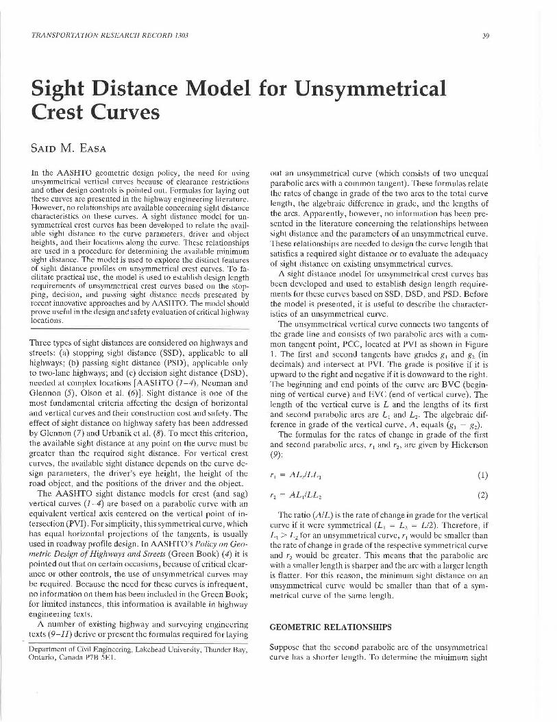
The unsymmetrical vertical curve connects two tangents of the grade line and consists of two parabolic arcs with a common tangent point, PCC, located at PVI as shown in Figure 1. The first and second tangents have grades g 1 and g2 (in decimals) and intersect at PVI. The grade is positive if it is upward to the right and negative if it is downward to the right. The beginning and end points of the curve are BVC (beginning of vertical curve) and EVC (end of vertical curve). The length of the vertical curve is L and the lengths of its first and second parabolic arcs are L 1 and L2 • The algebraic difference in grade of the vertical curve, A, equals (g1 - g2).

The formulas for the rates of change in grade of the first and second parabolic arcs, r 1 and r2 , are given by Hickerson (9):

(1)

(2)

The ratio (Al L) is the rate of change in grade for the vertical curve if it were symmetrical (L 1 = L 2 = L/2). Therefore, if L 1 > L 2 for an unsymmetrical curve, r1 would be smaller than the rate of change in grade of the respective symmetrical curve and r 2 would be greater. This means that the parabolic arc with a smaller length is sharper and the arc with a larger length is flatter. For this reason, the minimum sight distance on an unsymmetrical curve would be smaller than that of a symmetrical curve of the same length.

GEOMETRIC RELATIONSHIPS

Suppose that the second parabolic arc of the unsymmetrical curve has a shorter length. To determine the minimum sight

40 TRANSPORTATION RESEARCH RECORD 1303

g,

---obj eel

h,

I.. x12 •I ~ T

s

/ L,

FIGURE 1 Case 1: Object beyond EVC and driver on second arc.

distance, Sm, on the curve, the following five cases are considered:

•Case 1: Object beyond EVC and driver on second arc, • Case 2: Object beyond EVC and driver on first arc, • Case 3: Object beyond EVC and driver before BVC, • Case 4: Object before EVC and driver on first arc, and • Case 5: Object before EVC and driver before BVC.

The relationships between the available sight distance Sand the vertical curve length are derived for each of these cases for a specified location of the object. These relations are used later to determine Sm. The derivation is divided into the following three parts:

1. Derivation of the distance between the object and the tangent point of the line of sighl, S0 ;

2. Derivation of the distance between the driver and the tangent point of the line of sight, Sd; and

3. Obtaining the sight distance, S = S0 + Sd.

Case 1: Object Beyond EVC and Driver on Second Arc

In Case 1, the object lies beyond (or at) EVC and the driver is on the second arc. The distance between the object and EVC is denoted by T. Figure 1 shows the geometry of this case.

Component S0

On the basis of the property of a parabola, the vertical distance from EVC to the line of sight, y 1 , is given by

(3)

where x is the distance from EVC to the tangent point of the line of sight. Based on the similarity of the two triangles with

bases h2 and y1 , a quadratic equation in xis formed and the following relationship can be obtained:

x = -T + [T2 + (2hzfr2 )]112 (4)

The distance S0 , which equals T + x, becomes

Component Sd

On the basis of the property of a parabola, Sd is given by

Sight Distance S

The sight distance Sis the sum of the components of Equations 5 and 6, which gives

(7)

If the object is at EVC (T = 0), Equation 7 indicates that S will be constant and will remain so even if the object is before EVC, as long as both the driver and object are on the second arc.

Case 2: Object Beyond EVC and Driver on First Arc

The geometry of Case 2 is shown in Figure 2. Assume for now that the line of sight is tangent to the second arc. (The situation when the line of sight is tangent to the first arc is addressed later.)

Component S0

The derivation of S0

is similar to Case 1. Thus,

(8)

Easa 41

Line of sight

Driv:: __ /

ob)ect

h, g,

A s, s.

f• T .,,

s

L, L,

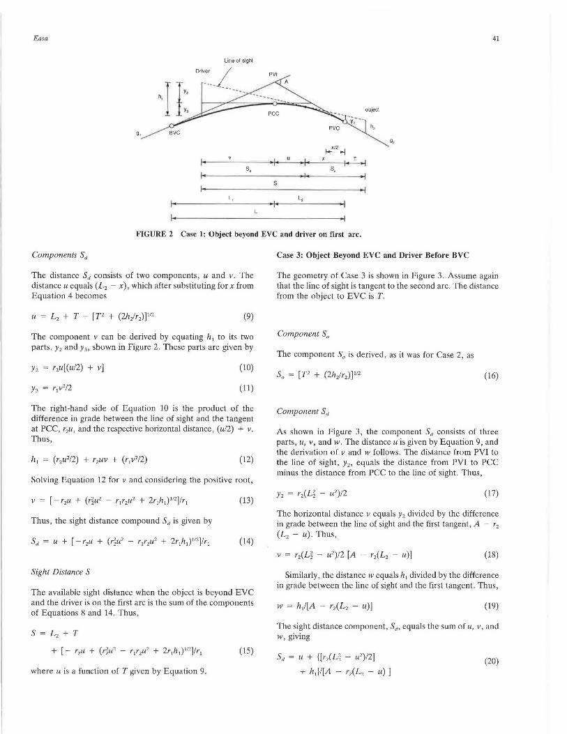
FIGURE 2 Case 1: Object beyond EVC and driver on first arc.

Components Sd

The distance Sd consists of two components, u and v. The distance u equals (L2 - x), which after substituting for x from Equation 4 becomes

(9)

The component v can be derived by equating h1 to its two parts, Y2 and y3 , shown in Figure 2. These parts are given by

y2 = r2u[(u/2) + v] (10)

(11)

The right-hand side of Equation 10 is the product of the difference in grade between the line of sight and the tangent at PCC, r2u, and the respective horizontal distance, (u/2) + v. Thus,

(12)

Solving Equation 12 for v and considering the positive root,

(13)

Thus, the sight distance compound Sd is given by

(14)

Sight Distance S

The available sight distance when the object is beyond EVC and the driver is on the first arc is the sum of the components of Equations 8 and 14. Thus,

(15)

where u is a function of T given by Equation 9.

Case 3: Object Beyond EVC and Driver Before BVC

The geometry of Case 3 is shown in Figure 3. Assume again that the line of sight is tangent to the second arc. The distance from the object to EVC is T.

Component S0

The component S0 is derived, as it was for Case 2, as

(16)

Component Sd

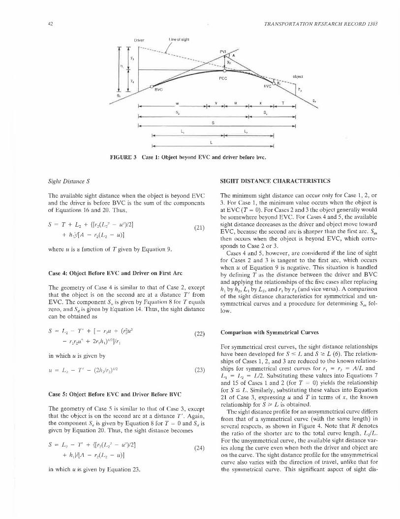
As shown in Figure 3, the component Sd consists of three parts, u, v, and w. The distance u is given by Equation 9, and the derivation of v and w follows. The distance from PVI to the line of sight, y2 , equals the distance from PVI to PCC minus the distance from PCC to the line of sight. Thus,

(17)

The horizontal distance v equals y2 divided by the difference in grade between the line of sight and the first tangent, A - r2

(L2 - u). Thus,

(18)

Similarly, the distance w equals h1 divided by the difference in grade between the line of sight and the first tangent. Thus,

(19)

The sight distance component, Sd, equals the sum of u, v, and w, giving

Sd = u + {[r2(L~ - u2)/2] (20) + h1}/[A - r2(L 2 - u) ]


Driv~~- ·-•••• _;ne of sighl

y, ---h,

object

g,

s, s.

s L, L,

L

FIGURE 3 Case 1: Object beyond EVC and driver before bvc.

Sight Distance S

The available sight distance when the object is beyond EVC and the driver is before BVC is the sum of the components of Equations 16 and 20. Thus ,

S = T + L2 + {[r2(Lz2 - u2)/2]

+ h1}/[A - r2(L 2 - u)]

where u is a function of T given by Equation 9.

Case 4: Object Before EVC and Driver on First Arc

(21)

The geometry of Case 4 is similar to that of Case 2, except that the object is on the second arc at a distance T' from EVC. The component S0 is given by El1ualiun 8 for T eyuals zero, and Sd is given by Equation 14. Thus, the sight distance can be obtained as

S = L 2 - T' + [ - r2u + Viui

- ririui + 2r1h 1)1'2]/r1

in which u is given by

u = Li - T' - (2hzfri) 112

Case 5: Object Before EVC and Driver Before BVC

(22)

(23)

The geometry of Case 5 is similar to that of Case 3, except that the object is on the second arc at a distance T'. Again, the component S0 is given by Equation 8 for T = 0 and Sd is given by Equation 20. Thus , the sight distance becomes

S = Li - T' + {[ri(Lii - u2)/2]

+ h 1}/[A - rz(L2 - u)]

in which u is given by Equation 23.

(24)

SIGHT DISTANCE CHARACTERISTICS

The minimum sight distance can occur only for Case 1, 2, or 3. For Case 1, the minimum value occurs when the object is at EVC (T = 0). For Cases 2 and 3 the object generally would be somewhere beyond EVC. For Cases 4 and 5, the available sight distance decreases as the driver and object move toward EVC, because the second arc is sharper than the first arc. Sm then occurs when the object is beyond EVC, which corresponds to Case 2 or 3.

Cases 4 and 5, however, are considered if the line of sight for Cases 2 and 3 is tangent to the first arc, which occurs when u of Equation 9 is negative. This situation is handled by defining T as the distance between the driver and BVC and applying the relationships of the five cases after replacing h 1 by h2 , Li by L 2 , and r 1 by r 2 (and vice versa). A comparison of the sight distance characteristics for symmetrical and unsymmetrical curves and a procedure for determining Sm follow.

Comparison with Symmetrical Curves

For symmetrical crest curves, the sight distance relationships have been developed for S :S Land S ;o:: L (6). The relationships of Cases 1, 2, and 3 are reduced to the known relationships for symmetrical crest curves for r 1 = r 2 = Al L and Li = L 2 = L/2. Substituting these values into Equations 7 and 15 of Cases 1 and 2 (for T = 0) yields the relationship for S :S L. Similarly, substituting these values into Equation 21 of Case 3, expressing u and Tin terms of x, the known relationship for S ;;,, L is obtained.

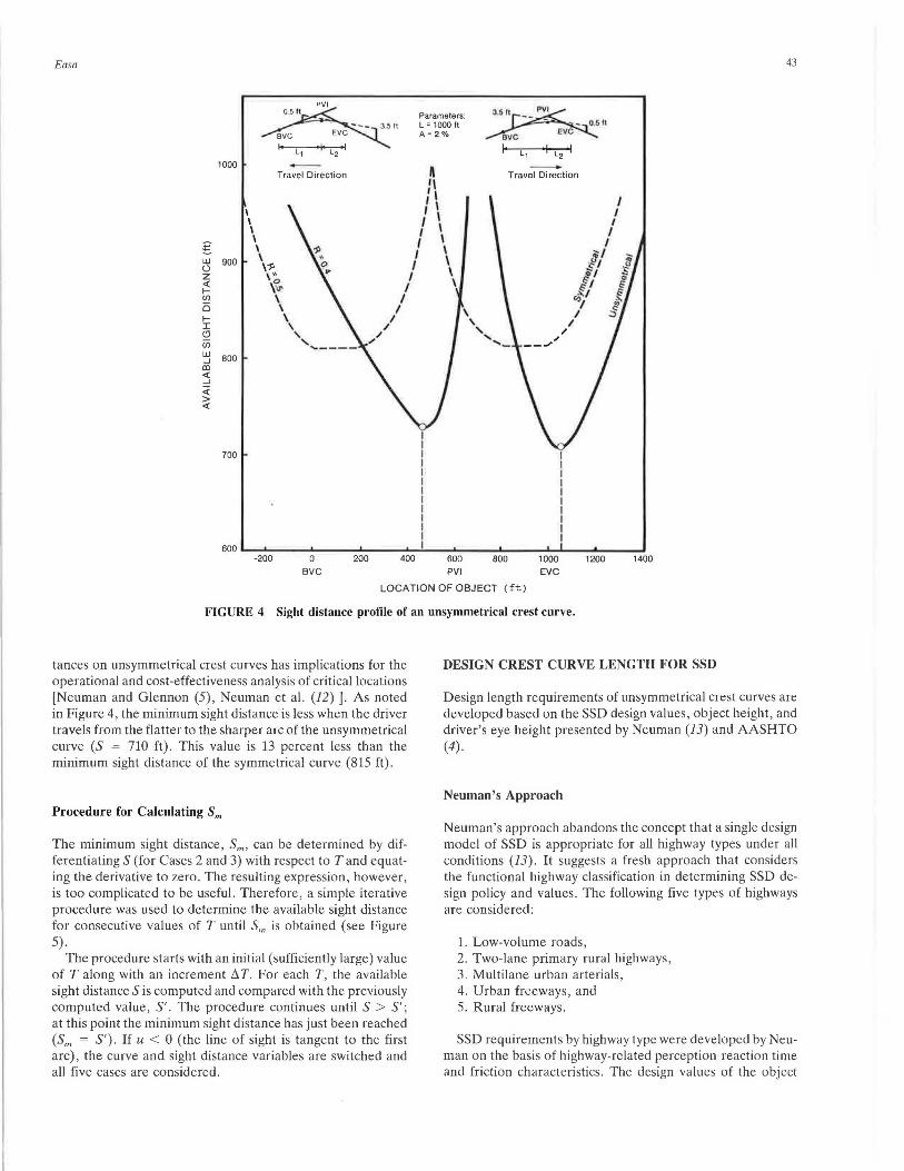
The sight distance profile for an unsymmetrical curve differs from that of a symmetrical curve (with the same length) in several respects, as shown in Figure 4. Note that R denotes the ratio of the shorter arc to the total curve length, Li L. For the unsymmetrical curve, the available sight distance varies along the curve even when both the driver and object are on the curve. The sight distance profile for the unsymmetrical curve also varies with the direction of travel, unlike that for the symmetrical curve. This significant aspect of sight dis-

Easa

1000 Travel Direction

I I \ \

'!:. \ w 900 \ (.) \-,l

Parameters: L = 1000 ft A= 2%

ft I\ '1 I I I I I I I I I I I \

-Travel Direction

I I I

I I ... ,

!1

43

z \ " <( \~

I \ I \

I l'

f / I-en \ 0 \ I- \ I \ CJ iii w 800 _J

ID <( _J

~ > <(

700

-200

' ' ...... ____

0 BVC

200

,,. I

I /

I I

400 600 PVI

800

__ _,,.

""1 I

I I ,,.

1000 EVC

1200 1400

LOCATION OF OBJECT (ft)

FIGURE 4 Sight distance profile or an unsymmetrical crest curve.

tances on unsymmetrical crest curves has implications for the operational and cost-effectiveness analysis of critical locations (Neuman and Glennon (5), Neuman et al. (12) ]. As noted in Figure 4, the minimum sight distance is less when the driver travels from the flatter to the sharper arc of the unsymmetrical curve (S = 710 ft). This value is 13 percent less than the minimum sight distance of the symmetrical curve (815 ft).

Procedure for Calculating S,,,

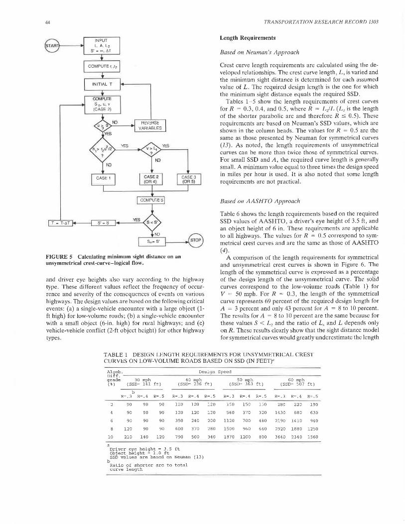
The minimum sight distance , S,,,, can be determined by differentiating S (for Cases 2 and 3) with respect to Tand equating the derivative to zero. The resulting expression, however, is too complicated to be useful. Therefore, a simple iterative procedure was used to determine the available sight distance for consecutive values of T until S'" is obtained (see Figure 5).

The procedure starts with an initial (sufficiently large) value of T along with an increment 11T. For each T, the available sight distance Sis computed and compared with the previously computed value, S'. The procedure continues until S > S' ; at this point the minimum sight distance has just been reached (Sm = S'). If u < 0 (the line of sight is tangent to the first arc), the curve and sight distance variables are switched and all five cases are considered.

DESIGN CREST CURVE LENGTH FOR SSD

Design length requirements of unsymmetrical crest curves are developed based on the SSD design values, object height, and driver's eye height presented by Neuman (13) and AASHTO (4).

Neuman's Approach

Neuman's approach abandons the concept that a single design model of SSD is appropriate for all highway types under all conditions (13). It suggests a fresh approach that considers the functional highway classification in determining SSD design policy and values. The following five types of highways are considered:

1. Low-volume roads, 2. Two-lane primary rural highways, 3. Multilane urban arterials, 4. Urban freeways, and 5. Rural freeways.

SSD requirements by highway type were developed by Neuman on the basis of highway-related perception-reaction time and friction characteristics. The design values of the object

44

T - T-AT

INPUT L, A, L2

S' - ~.AT

S' -s

REVERSE VARIABLES

Sm= S'

FIGURE 5 Calculating minimum sight distance on an unsymmetrical crest-curve-logical flow.

CASE3 (ORS)

and driver eye heights also vary according to the highway type. These different values reflect the frequency of occurrence and severity of the consequences of events on various highways . The design values are based on the following critical events : (a) a single-vehicle encounter with a large object (1-ft high) for low-volume roads; (b) a single-vehicle encounter with a small object (6-in. high) for rural highways ; and (c) vehicle-vehicle conflict (2-ft object height) for other highway types.

TRANSPORTATION RESEARCH RECORD 1303

Length Requirements

Based on Neuman's Approach

Crest curve length requirements are calculated using the developed relationships. The crest curve length, L, is varied and the minimum sight distance is determined for each assumed value of L The required design length is the one for which the minimum sight distance equals the required SSD.

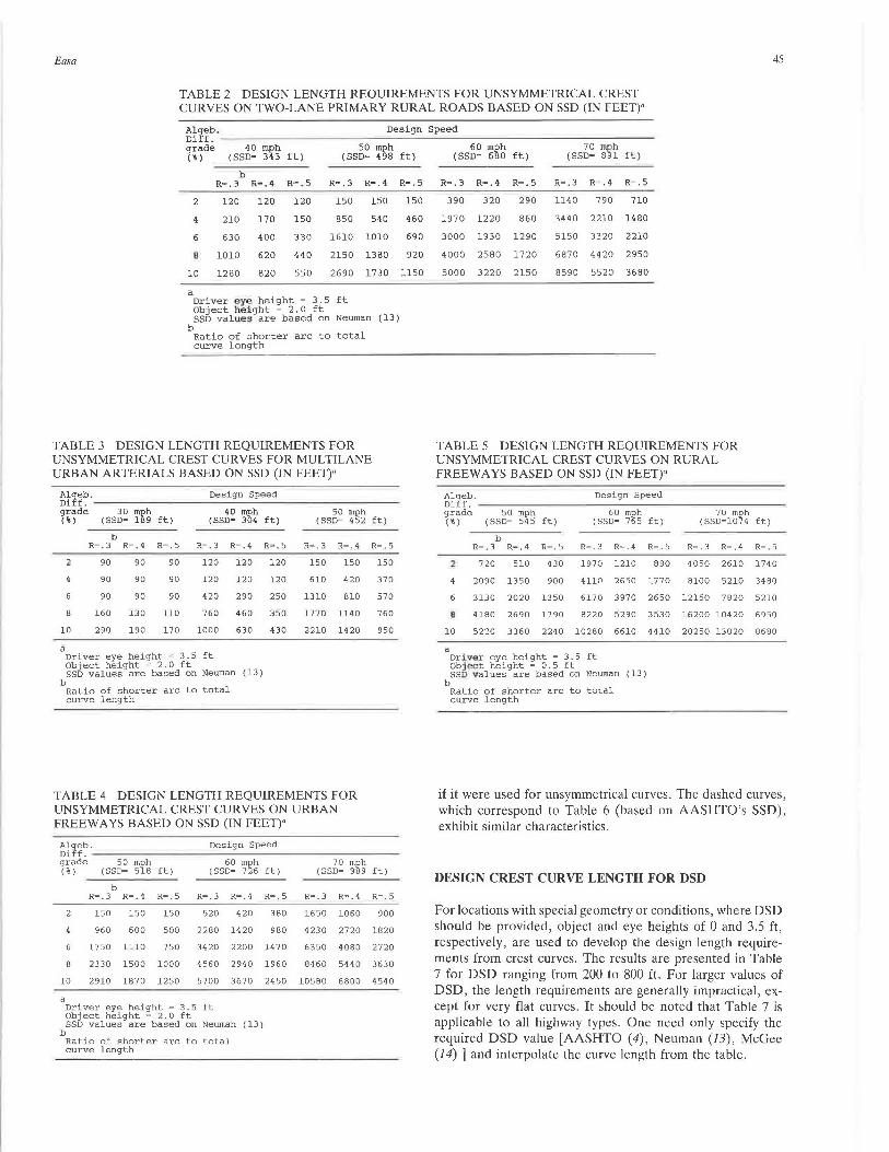
Tables 1-5 show the length requirements of crest curves for R = 0.3, 0.4 , and 0.5, where R = L zfL (L2 is the length of the shorter parabolic arc and therefore R :5 0.5). These requirements are based on Neuman's SSD values, which are shown in the column heads. The values for R = 0.5 are the same as those presented by Neuman for symmetrical curves (13). As noted, the length requirements of unsymmetrical curves can be more than twice those of symmetrical curves . For small SSD and A, the required curve length is generally small. A minimum value equal to three times the design speed in miles per hour is used. It is also noted that some length requirements are not practical.

Based on AASHTO Approach

Table 6 shows the length requirements based on the required SSD values of AASHTO, a driver's eye height of 3.5 ft, and an object height of 6 in . These requirements are applicable to all highways . The values for R = 0.5 correspond to symmetrical crest curves and are the same as those of AASHTO (4).

A comparison of the length requirements for symmetrical and unsymmetrical crest curves is shown in Figure 6. The length of the symmetrical curve is expressed as a percentage of the design length of the unsymmetrical curve. The solid curves correspond to the low-volume roads (Table 1) for V = 50 mph . For R = 0.3, the length of the symmetrical curve represents 69 percent of the required design length for A = 3 percent and only 43 percent for A = 8 to 10 percent. The results for A = 8 to 10 percent are the same because for these values S < L 2 and the ratio of Ls and L depends only on R. These results clearly show that the sight distance model for symmetrical curves would greatly underestimate the length

TABLE 1 DESIGN LENGTH REQUIREMENTS FOR UNSYMMETRICAL CREST CURVES ON LOW-VOLUME ROADS BASED ON SSD (IN FEET)"

Algeb. Design Speed Diff. grade 30 mph 40 mph 50 mph 60 mph ( %) (SSD- 141 ft) (SSD= 236 ft) (SSD~ 363 ft) (SSD= 507 ft)

b R=.3 R=.4 R=.5 R- .3 R=.4 R- .5 R- . 3 R=.4 R- . 5 R- .3 R=.4 R=.5

2 90 90 90 120 120 120 150 150 l'.:iO 280 220 190

4 90 90 90 120 120 120 560 370 320 1430 880 630

90 90 90 350 240 200 1120 700 480 2190 1410 940

8 120 90 90 600 370 280 1500 960 640 2920 1880 1250

10 210 140 120 790 500 340 1870 1200 800 3640 2340 1560

a Driver eye height= 3.5 ft Object height - 1.0 ft SSD values are based on Newnan (13)

b Ratio of shorter arc to total curve length

Easa 45

TABLE 2 DESIGN LENGTH REQUIREMENTS FOR UNSYMMETRICAL CREST CURVES ON TWO-LANE PRIMARY RURAL ROADS BASED ON SSD (IN FEET)"

Algeb , Design Speed Diff. ~~~~~~~~~~~~~~~~~~~~~~~~~~~~~~~~~ grade 40 mph (%) (SSD- 343 ft)

b

50 mph (SSD- 498 ft)



R-.3 R-.4 R-.5 R-.3 R- .4 R-.5 R-.3 R-.4 R- .5 R- .3 R-.4 R- .5

2 120 120 120 150 150 150 390 320 290 1140 790 710

4 210 170 150 850 540 460 1970 1220 860 3440 2210 1480

6 630 400 330 1610 1010 690 3000 1930 1290 5150 3320 2210

8 1010 620 440 2150 1380 920 4000 2580 1720 6870 4420 2950

10 1280 820 550 2690 1730 1150 5000 3220 2150 8590 5520 3680

a Driver eye height - 3.5 ft Object height - 2.0 ft SSD values are based on Neuman


TABLE 3 DESIGN LENGTH REQUIREMENTS FOR UNSYMMETRICAL CREST CURVES FOR MULTILANE URBAN ARTERIALS BASED ON SSD (IN FEET)"

(13)

t~tf~·~~~~~~~~~D_e_s_ig_n~S_p_e_ed~~~~~~~~~-grade 30 mph 40 mph (%) (SSD- 189 ft) (SSD- 304 ft)

b


R- .3 R-.4 R- .5 R- .3 R- .4 R-.5 R-.3 R- .4 R- .5

120 120 120

120 120 120

150 150 150

610 420 370

90

90

90

90

90

90

90

90

90

160 130 llO

420 290 250 1310 810 570

760 460 350 1770 1140 760

10 290 190 170 1000 630 430 2210 1420 950

a Driver eye height - 3.5 ft Object height - 2.0 ft SSD values are based on Neuman (13)


TABLE 4 DESIGN LENGTH REQUIREMENTS FOR UNSYMMETRICAL CREST CURVES ON URBAN FREEWAYS BASED ON SSD (IN FEET)"

Algeb. Design Speed Diff. ~~~~~~~~~~~~~~~~~~~~~~~ grade 50 mph (%) (SSD- 518 ft)

b



R- .3 R- .4 R- .5 R- .3 R- .4 R-.5 R- .3 R-.4 R-.5

150 150 150 520 420

4 960 600 500 2280 1420

1750 1110 750 3420 2200

8 2330 1500 1000 4560 2940

10 2910 1870 1250 5700 3670

a Driver eye height - 3.5 ft Object height - 2.0 ft SSD values are based on Neuman (13)


380

980

1470

1960

2450

1650

4230

6350

8460

10580

1060

2720

4080

5440

6800

900

1820

2720

3630

4540

TABLE 5 DESIGN LENGTH REQUIREMENTS FOR UNSYMMETRICAL CREST CURVES ON RURAL FREEWAYS BASED ON SSD (IN FEET)"

Algeb. Design Speed Diff. ~~~~~~~~~~~~~~~~~~~~~~~ grade 50 mph 60 mph

(SSD- 765 ft) 70 mph

(SSD-1074 ft) (%) (SSD- 545 ft)

b R-.3 R-.4 R-.5 R- .3 R-.4 R- .5 R- .3 R- .4 R- .5

2 720 510 430 1970 1210 890 4050 2610 1740

2090 1350 900 4110 2650 1770 8100 5210 3480

6 3130 2020 1350 6170 3970 2650 12150 7820 5210

8 4180 2690 1790 8220 5290 3530 16200 10420 6950

10 5220 3360 2240 10280 6610 4410 20250 13020 8680

a Driver eye height - 3.5 ft Object height - 0.5 ft SSO values are based on Neuman (13)


if it were used for unsymmetrical curves. The dashed curves, which correspond to Table 6 (based on AASHTO's SSD), exhibit similar characteristics.

DESIGN CREST CURVE LENGTH FOR DSD

For locations with special geometry or conditions, where DSD should be provided, object and eye heights of 0 and 3.5 ft, respectively, are used to develop the design length requirements from crest curves. The results are presented in Table 7 for DSD ranging from 200 to 800 ft. For larger values of DSD, the length requirements are generally impractical, except for very flat curves. It should be noted that Table 7 is applicable to all highway types. One need only specify the required DSD value [AASHTO (4), Neuman (13), McGee (14) ] and interpolate the curve length from the table.

TABLE 6 DESIGN LENGTH REQUIREMENTS FOR UNSYMMETRICAL CREST CURVES ON ALL HIGHWAYS BASED ON SSD OF AASHTO"

Algeb , Diff.

Design Speed

grade 20 mph 30 mph 40 mph 50 mph 60 mph 70 mph (%) (SSD- 125 ft) (SSD- 200 ft) (SSD- 275 ft) (SSD- 400 ft) (SSD- 525 ft) (SSD- 625

b b R- .3 R- .4 R- .5 R-.3 R-.4 R- .5 R- .3 R-.4 R-.5 R-.3 R- .4 R- .5 R- .3 R-.4 R- .5 R- .3

60 60 60 90 90 90 120 120 120 210 160 150 630 460 390 1120

60 60 60 110 90 90 370 260 220 llOO 680 490 1940 1250 830 2750

6 60 60 60 330 220 lBO 790 490 350 1690 1090 730 2910 1870 1250 4120

8 140 100 90 550 340 250 1070 690 460 2250 1450 970 3880 2490 1660 5490

10 230 150 120 710 450 310 1330 860 570 2810 1810 1210 4840 3120 2080 6860

a Driver eye height - 3.5 ft Note: curve lengths are expressed in feet.

b Object height -o.5 ft

Ratio of shorter curve length

arc to total

100

90

80

Ls T(%)

70

60

50

40 0.2

Neuman (l VR)

AASHTO

0.3 0.4

FIGURE 6 Comparison of length requirements of symmetrical and unsymmetrical crest curves (V = 50 mph).

0 .5

TABLE 7 DESIGN LENGTH REQUIREMENTS FOR UNSYMMETRICAL CREST CURVES ON ALL HIGHWAYS BASED ON DSD"

Algeb . Diff.

Decision Sight Distance (ft)

grade (%) 200 400 600 800

b R-.3 R-.4 R-.5 R-.3 R- .4 R- .5 R-.3 R- .4 R-.5 R- .3 R-.4 R-.5

2 90 70 50 1020 640 460 2400 1550 1030 4270 2750 1830

4 '.>lU :J~U ~:JU ~140 UHO 920 4800 3090 2060 8540 5490 3660

6 800 520 350 3200 2060 1380 7200 4630 3090 12800 8230 5490

8 1070 690 460 4270 2750 1830 9600 6180 4120 17070 10980 7320

10 1340 860 580 5340 3430 2290 12000 7720 5150 21340 13720 9150

a Driver eye height - 3.5 Object height - O ft

ft Note: curve lengths are expressed in feet.


R-.4

720

1770

2650

3530

4410

ft)

R- .5

590

ll80

1770

2360

2940

Easa 47

TABLE 8 DESIGN LENGTH REQUIREMENTS FOR UNSYMMETRICAL CREST CURVES BASED ON PSD (IN FEET)"

Algeb. Deeiqn Speed Diff. grade 20 mph 30 mph 40 mph

<'> d

R• .3 R=.4 R=.S R=.3 R=.4 R=.S R=.3 R=.4 R=.S

Paeeenger car Passing Paesenger c.u:h

(PSD= 325 ft) (PSO= 525 ft) (PSO= 700 ft)

2 60 60 60 90 90 90 120 120 120 4 60 60 60 360 300 280 1120 710 630 6 180 150 140 1090 660 ' 540 2220 1380 960 8 430 290 270 1660 1040 720 2960 1910 1270

10 720 440 350 2080 1340 900 3700 23BO 1590

Paeeanger car Passing TrucJc1>

(PSD= 350 ft) (PSO= 575 ft) (PSD= 800 ft)

2 60 60 60 90 90 90 120 120 120 4 60 60 60 530 410 3BO 1710 1040 B30 6 240 200 190 1400 BSO 650 1900 1B60 1250 8 560 360 320 2000 1280 860 3870 2490 1660

10 B80 530 400 2500 1610 1070 4830 3110 2070

Truck Passing Passenger car0

(PSD= 350 ft) (PSD= 600 ft) (PSD= 875 ft)

2 60 60 60 90 90 90 120 120 120 4 60 60 60 220 180 160 1170 BOD 710 6 60 60 60 B70 580 510 2540 1570 1110 8 250 200 lBO 1540 940 700 3440 2210 l4BO

10 470 320 290 2020 12BO 870 4300 2760 1840

Truck Paeeing Truck0


2 60 60 60 90 90 90 120 120 120 4 60 60 60 430 350 310 1710 lOBO 910 6 60 60 60 1280 BOO 660 3200 2020 13BO 8 250 200 180 2030 1260 880 4270 2750 1830

10 470 320 290 2560 1650 1100 5340 3430 2290

a PSD values are based on Harwood and Glennon (15)

b Driver eye height - 3.5 ft Object height - 4.25 ft

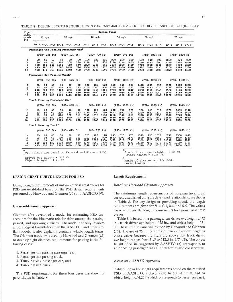
DESIGN CREST CURVE LENGTH FOR PSD

Design length requirements of unsymmetrical crest curves for PSD are established based on the PSD design requirements presented by Harwood and Glennon (15) and AASHTO (4).

Harwood-Glennon Approach

Glennon (16) developed a model for estimating PSD that accounts for the kinematic relationships among the passing, passed, and opposing vehicles . The model not only involves a more logical formulation than the AASHTO and other similar models, it also explicitly contains vehicle length terms. The Glennon model was used by Harwood and Glennon (15) to develop sight distance requirements for passing in the following cases:

1. Passenger car passing passenger car, 2. Passenger car passing truck, 3. Truck passing passenger car, and 4. Truck passing truck.

The PSD requirements for these four cases are shown in parentheses in Table 8.

so mph 60 mph 70 mph

R=.3 R=.4 R=.S R=.3 R• .4 R=.S R•.3 R=.4 R=.S

(PSD= 875 ft) (PSD• 1025 ft) (PSO• 1200 ft)

260 220 200 650 540 500 1250 920 850 2180 1320 1000 3160 1960 1360 4350 2790 1870 3470 2230 1490 4760 3060 2040 6520 4200 2800 4630 2980 1990 6350 4080 2720 8700 5590 3730 5780 3720 2480 7930 5100 3400 10870 6990 4660


650 540 500 1470 1030 950 2520 1570 1350 3160 1960 1360 4720 3030 2030 6350 40BO 2720 4760 3060 2040 7080 4550 3040 9520 6120 40BO 6350 4080 2720 9440 6070 4050 12690 Bl60 5440 7930 5100 3400 11790 75BO 5060 15870 10200 6800


230 190 170 920 740 670 1770 1300 1170 2610 1590 1220 4220 2620 1820 5930 3BOD 2540 4260 2740 1B30 6370 4090 2730 8890 5720 3810 5680 3650 2440 B490 5460 3640 11850 7620 50BO 7100 4570 3050 10610 6B20 4550 14810 9520 6350

(PSO= 1275 ft) (PSD= 1575 ft) (PSD= 1875 ft)

640 3570 5470 7300 9120

520 2190 3520 4690 5860

c

470 1570 1190 1070 2990 1930 1570 5570 3560 2390 7B90 5070 2350 B350 5370 35BO 11830 7610 3130 11130 7160 4770 15770 10140 3910 13910 B950 5970 19720 126BO

Truck driver eye height= 6.25 ft Object height= 4.25 ft

dRatio of shorter arc to total curve length

Length Requirements

Based on Harwood-Glennon Approach

1670 3380 5070 6760 B450

The minimum length requirements of unsymmetrical crest curves, established using the developed relationships, are shown in Table 8. For any design or prevailing speed, the length requirements are given for R = 0.3, 0.4, and 0.5. The values for R = 0.5 are the length requirements for symmetrical crest curves.

Table 8 is based on a passenger car driver eye height of 42 in., truck driver eye height of 75 in., and object height of 51 in. These are the same values used by Harwood and Glennon (15). The use of 75 in. to represent truck driver eye height is conservative because the literature shows that truck driver eye height ranges from 71.5 to 112.5 in. (17-19). The object height of 51 in. suggested by AASHTO (4) corresponds to an opposing passenger car and therefore is also conservative.

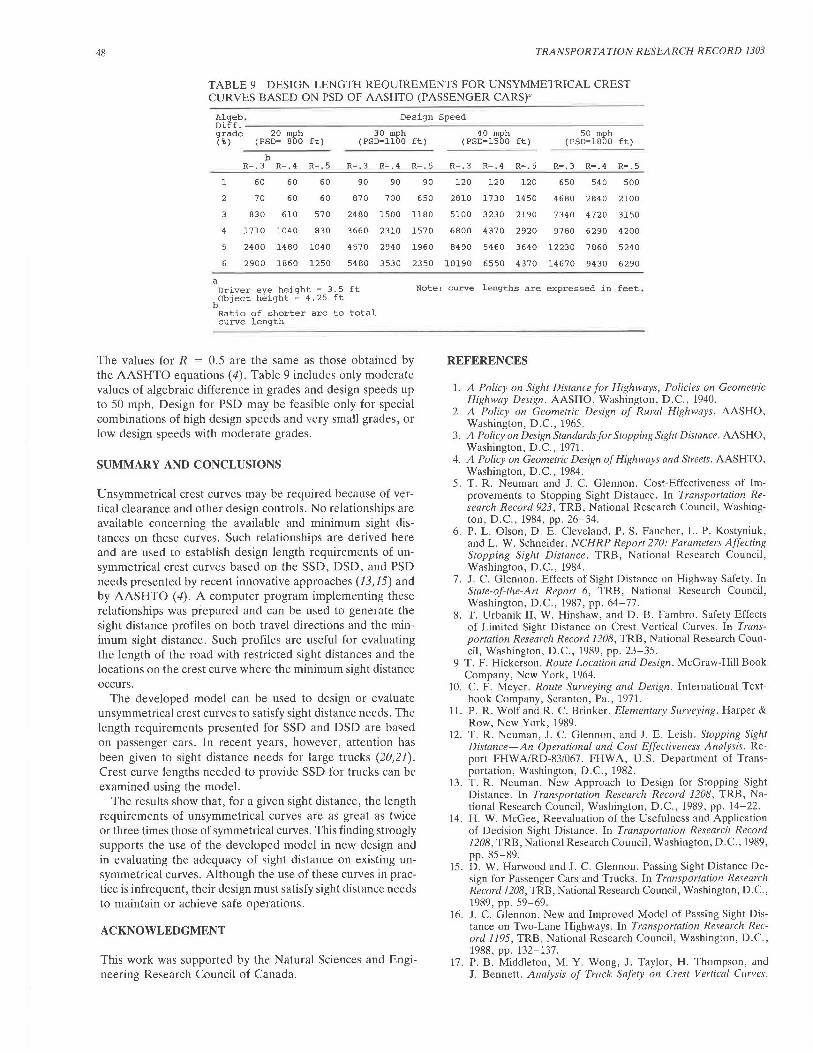
Based on AASHTO Approach

Table 9 shows the length requirements based on the required PSD of AASHTO, a driver's eye height of 3.5 ft, and an object height of 4.25 ft (which corresponds to passenger cars).


TABLE 9 DESIGN LENGTH REQUIREMENTS FOR UNSYMMETRICAL CREST CURVES BASED ON PSD OF AASHTO (PASSENGER CARS)"

Algeb . Design Speed Diff. grade 20 mph 30 mph 40 mph 50 mph (%) (PSD- 800 ft) (PSD-llOO ft) (PSD-1500 ft) (PSD- 1800 ft)

b R-.3 R-.4 R-.5 R-.3 R-.4 R-.5 R-.3 R-.4 R-.5 R-.3 R-.4 R-.5

1 60 60 60 90 90 90 120 120 120 650 540 500

2 70 60 60 870 700 650 2810 1730 1450 4680 2840 2100

3 830 610 570 2480 1500 ll80 5100 3230 2190 7340 4720 3150

4 1710 1040 830 3660 2310 1570 6800 4370 2920 9780 6290 4200

5 2400 1480 1040 4570 2940 1960 8490 5460 3640 12230 7860 5240

6 2900 1860 1250 5480 3530 2350 10190 6550 4370 14670 9430 6290

a Driver eye height - 3.5 ft

bObject height - 4.25 ft Note: curve lengths are expressed in feet .

Ratio of shorter arc to total curve length

The values for R = 0.5 are the same as those obtained by the AASHTO equations (4). Table 9 includes only moderate values of algebraic difference in grades and design speeds up to 50 mph. Design for PSD may be feasible only for special combinations of high design speeds and very small grades, or low design speeds with moderate grades.

SUMMARY AND CONCLUSIONS

Unsymmetrical crest curves may be required because of vertical clearance and other design controls. No relationships are available concerning the available and minimum sight distances on these curves. Such relationships are derived here and are used to establish design length requirements of unsymmetrical crest curves based on the SSD, DSD, and PSD needs presented by recent innovative approaches (13,15) and by AASHTO (4). A computer program implementing these relationships was prepared and can be used to generate the sight distance profiles on both travel directions and the minimum sight distance. Such profiles are useful for evaluating the length of the road with restricted sight distances and the locations on the crest curve where the minimum sight distance occurs.

The developed model can be used to design or evaluate unsymmetrical crest curves to satisfy sight distance needs. The length requirements presented for SSD and DSD are based on passenger cars. In recent years, however, attention has been given to sight distance needs for large trucks (20,21). Crest curve lengths needed to provide SSD for trucks can be examined using the model.

The results show that, for a given sight distance, the length requirements of unsymmetrical curves are as great as twice or three times those of symmetrical curves. This finding strongly supports the use of the developed model in new design and in evaluating the adequacy of sight distance on existing unsymmetrical curves. Although the use of these curves in practice is infrequent, their design must satisfy sight distance needs to maintain or achieve safe operations.

ACKNOWLEDGMENT

This work was supported by the Natural Sciences and Engineering Research Council of Canada.

REFERENCES

1. A Policy on Sight Distance for Highways, Policies on Geometric Highway Design. AASHO, Washington, D.C., 1940.

2. A Policy on Geometric Design of Rural Highways, AASHO, Washington, D.C., 1965.

3. A Policy on Design Standards for Stopping Sight Distance. AASHO , Washington, D.C., 1971.

4. A Policy on Geometric Design of Highways and Streets. AASHTO, Washington, D.C., 1984.

5 . T. R. Neuman and J. C. Glennon. Cost-Effectiveness of Improvements to Stopping Sight Distance. In Transportation Research Record 923, TRB, National Research Council, Washington, D.C., 1984, pp. 26-34.

6. P. L. Olson, D. E. Cleveland, P. S. Fancher, L. P. Kostyniuk, and L. W. Schneider. NCHRP Report 270: Parameters Affecting Stopping Sight Distance. TRB, National Research Council, Washington, D.C., 1984.

7. J. C. Glennon. Effects of Sight Distance on Highway Safety. In State-of-the-Art Report 6, TRB, National Research Council, Washington, D.C., 1987, pp. 64-77.

8. 'l'. Urbanik II, W. Hinshaw, and D. B. Fambro. Safety Effects of Limited Sight Distance on Crest Vertical Curves. In Transportation Research Record 1208, TRB, National Research Council, Washington, D.C., 1989, pp. 23-35.

9 T. F. Hickerson. Route Location and Design. McGraw-Hill Book Company, New York, 1964.

10. C. F. Meyer. Route Surveying and Design. International Textbook Company, Scranton, Pa., 1971.

11. P. R. Wolf and R. C. Brinker. Elementary Surveying. Harper & Row, New York, 1989.

12. T. R. Neuman, J. C. Glennon, and J. E. Leish . Stopping Sight Distance-An Operational and Cost Effectiveness Analysis. Report FHWA/RD-83/067. FHWA, U.S. Department of Transportation, Washington, D.C., 1982.

13. T. R. Neuman. New Approach to Design for Stopping Sight Distance. In Transportation Research Record 1208, TRB, National Research Council, Washington, D.C., 1989, pp. 14-22.

14. H. W. McGee, Reevaluation of the Usefulness and Application of Decision Sight Distance. In Transportation Research Record 1208, TRB, National Research Council, Washington, D.C., 1989, pp. 85-89.

15. D. W. Harwood and J. C. Glennon. Passing Sight Distance Design for Passenger Cars and Trucks. In Transportation Research Record 1208, TRB, National Research Council, Washington, D.C., 1989, pp. 59-69.

16. J. C. Glennon. New and Improved Model of Passing Sight Distance on Two-Lane Highways. In Transportation Research Record 1195, TRB, National Research Council, Washington, D.C., 1988, pp. 132-137.

17. P. B. Middleton, M. Y. Wong, J. Taylor, H. Thompson, and J. Bennett. Analysis of Truck Safety on Crest Vertical Curves.

Easa

Report FHWA/RD-86/060. FHWA , U.S. Department of Transportation , Washington, D.C., 1983.

18. J . W. Burger and M. U. Mulholland. Plane and Convex Mirror Sizes for Small to Large Trucks. NHTSA, U.S. Department of Transportation, Washington, D.C., 1982.

19. Urban Behavioral Research Associates. The Investigation of Driver Eye Height and Field of Vision . FHWA , U.S. Department of Transportation, Washington, D.C., 1978.

20. P. S. Fancher. Sight Distance Problems Related to Large Trucks. In Transportation Research Record 1052, TRB, National Research Council, Washington, D.C., 1986, pp . 29-35.

21. D. W. Harwood, W. D. Glauz, and J . M. Mason, Jr. Stopping Sight Distance Design for Large Trucks. In Transportation Research Record 1208, TRB , National Research Council , Washington, D.C., 1989, pp. 36-46.

DISCUSSION

DAVID L. GUELL Department of Civil Engineering, University of Missouri-Columbia, Columbia, Mo. 65211.

Easa has added to the knowledge of sight distance on vertical curves with this paper. The ability to develop sight distance profiles, as shown in Figure 4, will be valuable in assessing sight distance conditions on existing highways .

This discussion is concerned with the design requirements for unsymmetrical crest vertical curves, and in particular the length of curve necessary to provide a specified length of sight distance. In keeping with the nomenclature of the paper (Figure 1), an unsymmetrical vertical curve is made up of two symmetrical vertical curves of length L 1 and L 2 (where L1 > L2)

with the common point PCC under the PVI. A line tangent to the curve at PCC is parallel to a line connecting BVC to EVC and has a grade g3 given by

g1L1 + g1L2 g3 =

Li+ Lz (25)

The algebraic difference in grade for the unsymmetrical vertical curve is A equal to g2 - g1 • Note that this is the negative of A as given in the paper. The algebraic differences in grades of the two symmetrical curves are given by

(26)

(27)

In this discussion , g and A are given in percent .

49

The symmetrical vertical curve of length L 2 is the critical one for sight distance because it is the shorter of the two. Therefore the length of this curve must satisfy the design requirement that

(28)

where K is the rate of vertical curvature as given, for example, in Tables III-40 and III-41 of AASHTO (1) for stopping and passing sight distance. Substituting g3 from Equation 25 into A 2 in Equation 27 and recognizing that L, plus L2 is equal to L, the total length of the unsymmetrical curve, gives

(29)

Substituting L = L 2/R, as defined by the author, into Equation 29 and then substituting this A 2 into Equation 28 gives

L2 > KA·(l - R) (30)

Substitution into L = L 2/R gives

L > KA·(l - R)IR (31)

Equation 30 gives the required length of the shorter symmetrical vertical curve, and Equation 31 gives the required total length of the unsymmetrical curve in terms of parameters familiar to designers and the additional parameter R:

A = algebraic difference in grade, K = required rate of vertical curvature as given in AASHTO

tables (J), and R = ratio of length of shorter symmetrical curve to total

length of the unsymmetrical curve.

It should be noted that when using the tabulated values of K as given by AASHTO (1) with small values of A, the calculated length of the vertical curve is greater than actually required for sight distance. This occurs when the sight distance is greater than the required length of the shorter symmetrical vertical curve. For this reason the values of L computed by Equation 31 will be greater than the values given in the paper in Tables 6 and 9 for small values of A. Also note that the author did not used the tabulated K-values in AASHTO (1) Tables 111-40 and 111-41 associated with the design speeds in the author's Tables 6 and 9. The corresponding K-values for the paper's sight distances can be determined from AASHTO

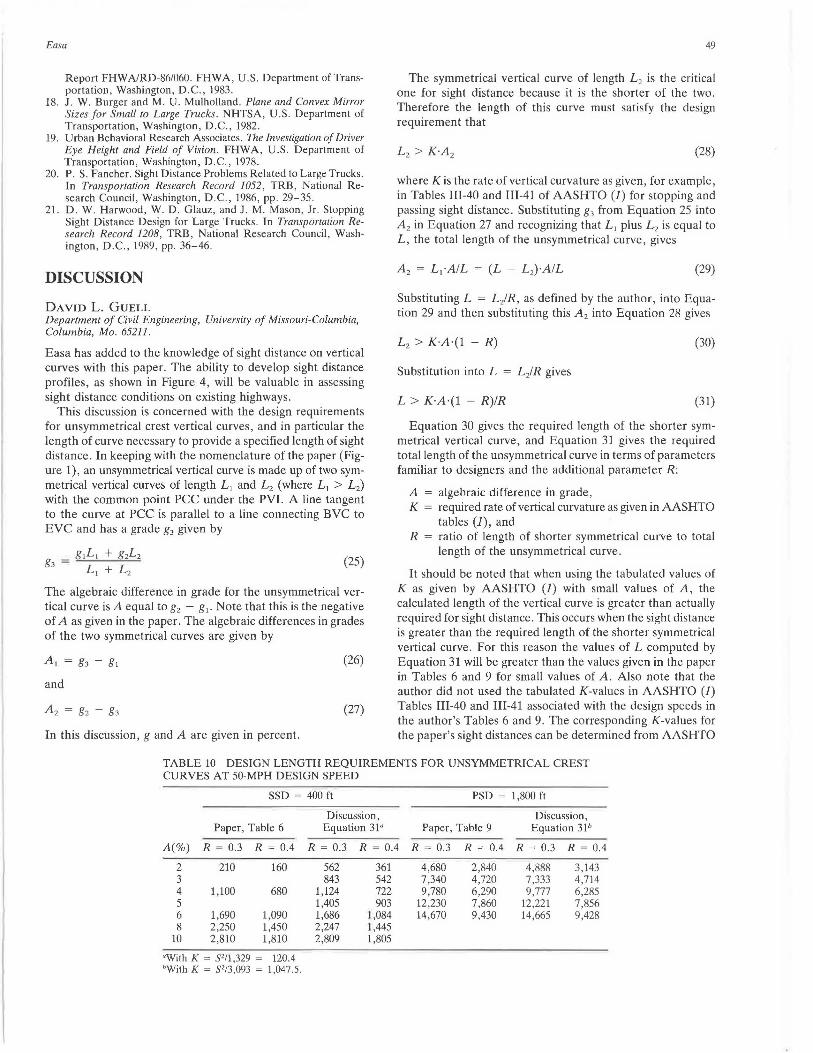
TABLE 10 DESIGN LENGTH REQUIREMENTS FOR UNSYMMETRICAL CREST CURVES AT 50-MPH DESIGN SPEED

SSD = 400 ft PSD = 1,800 ft

Discussion, Discussion , Paper, Table 6 Equation 31" Paper, Table 9 Equation 31•

A(o/o) R = 0.3 R = 0.4 R = 0.3 R = 0.4 R = 0.3 R = 0.4 R = 0.3 R = 0.4

2 210 160 562 361 4,680 2,840 4,888 3,143 3 843 542 7,340 4,720 7,333 4,714 4 1,100 680 1,124 722 9,780 6,290 9,777 6,285 5 1,405 903 12,230 7,860 12,221 7,856 6 1,690 1,090 1,686 J ,084 14,670 9,430 14,665 9,428 8 2,250 1,450 2,247 J ,445

10 2,810 1,810 2,809 1,805

"With K = 52/1,329 = 120.4 bWith K = 52/3,093 = 1,047.5.

50

Equation 3 for stopping sight distance (K = S2/1329) (1, p. 283) and Equation 5 for passing sight distance (K = S2/3093) (1, p. 288).

Table 10 compares the design length for unsymmetrical vertical curves as determined by the method of the paper and the method of this discussion for 50-mph design speed. The lengths are essentially the same except for small values of A.

REFERENCE

1. A Policy on Geometric Design of Highways and Streets. AASHTO, Washington , D.C. , 1990.

AUTHOR'S CLOSURE

The author thanks Professor Guell for his interest in the paper and for his thoughtful comments regarding establishment of the design length requirements of unsymmetrical crest curves based on the shorter arc.

The formula derived in his discussion for establishing length requirements (Equation 31) assumes that both the driver and object are on the shorter arc, which corresponds to Case 1 of the paper. The discussion indicates that the lengths calculated using this formula will be greater than actually required when A is small. The purpose of this closure is twofold: (a) to derive a general expression for Equation 31 and the condition for applying it, and (b) to show that this equation may overestimate the length requirements even when A is large.

For Case 1, the minimum sight distance, Sm, occurs when the object is at EVC. Setting T = 0, substituting for r2 from Equation 2 into Equation 7, and nothing that Li = (1 - R)L, one obtains

(32)

where the term in brackets equals the rate of vertical curvature K (Equation 32 is similar to Equation 30). Note that A is defined in the paper as gi - g2 , which always yields a positive value for crest curves. Since L2 = LR, Equation 32 gives

(33)

which is a general expression for the length requirements for Case 1 (Equation 33 is similar to Equation 3). For Equation 33 to be valid, however, S,,, must be less than or equal to L2 .

That is,

from which

A 2

f{2/7i)'n + (~1 2) 112 ]2 (1 - R)S,.,

(34)

(35)

Equation 35 is the condition of A for which Equation 33 gives exact length requirements . For values of A less than those

TRANSPORTATION RESEARCH RECORD 1303

16

14

l 12 (Val id r eg ion for Eq. 2)

<(

w 0 <( a: 10 (.')

~ w 0 z w 8 a: w IJ.. IJ..

0 0 <( 6 a: m w

I I I I I I

(.') _, <( I

4

2

-g I I I " I I c.

-a_I (/) -3. I -a_ I "3.1 c El E l El EI OJ

'fil ~I ~ I £ 1 R I 0 I I I I

I I I I 0

0 100 200 300 400 500 600

MINIMUM SIGHT DISTANCE. Sm {ft)

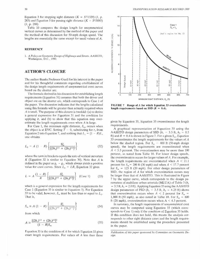
FIGURE 7 Range of A for which Equation 33 overestimates length requirements based on SSD (R = 0.4).

700

given by Equation 35, Equation 33 overestimates the length requirements.

A graphical representation of Equation 35 using the AASHTO design parameters of SSD (hi = 3.5 ft, h2 = 0.5 ft) and R = 0.4 is shown in Figure 7. For a given S,,,, Equation 33 overestimates the length requirements for the values of A below the shaded region. For Sm = 400 ft (50-mph design speed), the length requirements are overestimated when A < 5.5 percent. The overestimation may be 111u1e Lhau 100 percent, as noted from Table 10. For lower design speeds, the overestimation occurs for larger values of A. For example, the length requirements are overestimated when A < 11.1 percent for S,,, = 200 ft (30 mph) and when A < 17. 7 percent for Sm = 125 ft (20 mph). For other design parameters of SSD, the region of A for which overestimation occurs may be larger than that of AASHTO. This is illustrated in Figure 7 by the upper curve, which corresponds to the design parameters of multilane urban arterials (MLUA) of Table 3 (h, = 3.5 ft, h2 = 2.0 ft) . Applying Equation 35 using the AASHTO design parameters of PSD (h, = 3.5 ft, h2 = 4.25 ft) shows that overestimation occurs when A < 2 percent for S,,, = 1,800 ft (50 mph), as also noted in Table 10. For S,,, = 800 ft (20 mph), overestimation occurs when A < 4.5 percent.

In summary, the length requirements of unsymmetrical crest curves may be computed using Equation 33 (which corresponds to Case 1) only if the condition of Equation 35 holds. If this condition does not hold, this means the analysis corresponds to other sight distance cases and the length requirements should be established using the procedure presented in the paper.

Publicalion of !his paper sponsored by Commiltee on Geomelric Design.

sight distance model for unsymmetrical crest...

Documents