should fast-moving capital in crowded trades be … annual meetings...should fast-moving capital in...

Should Fast-Moving Capital in Crowded Trades Be Avoided?1

Albert J. Menkveld

First version: December 13, 2013This version: January 15, 2015

1Albert J. Menkveld, VU University Amsterdam, FEWEB, De Boelelaan 1105, 1081 HV, Amsterdam, Netherlands,tel +31 20 598 6130, [email protected] and Tinbergen Institute. I thank Matthieu Bouvard, Hans Degryse,Bernard Dumas, Thierry Foucault, Denis Gromb, Björn Hagströmer, Wenqian Huang, Vincent van Kervel, ThorstenKoeppl, Péter Kondor, Konrad Raff, Wolf Wagner, Bart Zhou Yueshen, Marius Zoican, and seminar/conference par-ticipants at INSEAD for comments. I am grateful to EMCF for in-depth discussions about clearing.

mailto:[email protected]

Abstract

Should Fast-Moving Capital in Crowded Trades Be Avoided?

If all intermediaries enter the same market-making “bet” on the same side, fast-moving capital gets tiedup in a crowded trade. This creates systemic risk for a central clearing party (CCP) since multiple tradersmight default when the bet turns (extremely) sour. The CCP then has to unwind the inherited portfolios ina market without fast-moving capital and potentially pay a fire sale premium. Equilibrium analysis revealsthat crowded trades are socially costly, but so is the other extreme: perfect diversity. Surprisingly, the CCPneeds most collateral in the latter case, either as margin or to fill the default fund.

Mandatory central clearing removes counterparty risk from derivatives trading and concentrates it in the

central clearing party, CCP (Koeppl and Monnet, 2014). The CCP becomes a “systemic node” in the new

financial architecture. Its risk management becomes critically important (Bernanke, 2011). We focus on two

standard tools used by CCPs: margins and the default fund.1

This paper analyzes a trade economy with a CCP that maintains a default fund large enough to stay

afloat at all times. The fund should be able to absorb losses in the trade portfolios it inherits from clearing

members in default. These are mark-to-market losses, net of the margin posted by the member. The default

fund should be able to pay for these losses but also for additional losses in case the CCP needs to unwind

these portfolios in the market at fire sale prices. The paper’s main contribution is an equilibrium analysis

of liquidation cost in “extreme but plausible” market conditions (BIS-IOSCO, 2004; ESMA, 2012, Section

4.5.4 and Article 41, respectively).

The constraint of a large enough clearing fund creates a “self-financing” financial market infrastructure

(FMI). This exogenous constraint is admittedly extreme, but serves to identify the social cost and benefit

of tying up capital either through margin or through a contribution to the default fund. A discussion of

“waterfall” default beyond the default fund is outside the scope of this paper (Duffie, 2010a, 2014; BIS-

IOSCO, 2014).

The paper’s focus is exclusively on CCP risk as caused by default of intermediaries; in the model end-

users do not default by assumption. Intermediaries are therefore the only ones who need to post margin

and contribute to the default fund. This is in line with recently published guidelines that stipulate that

only “financial firms and systemically important non-financial entities” need to post margin (BCBS and

IOSCO, 2013, 2.4, p. 9). These are often highly leveraged institutions that operate under limited liability.

1Resolution schemes in case of (multiple) member default and the size of a default fund in particular are quickly taking centralstage in the public discussion on central clearing. JPMorgan recently called for a larger fund. See “JPMorgan tells clearers to buildbigger buffers,” Financial Times, September 11, 2014.

1

They represent “fast-moving capital” in the sense that they can quickly build up extremely large speculative

positions. These features make them systemically important as their default could trigger CCP default. A

second reason for their importance is that they are the ones a CCP relies on when it needs to liquidate trade

portfolios it inherits from members in default. CCPs need to liquidate within a pre-specified so-called close-

out period and therefore cannot avoid fire sales by simply “waiting it out.” This period is relatively short,

typically in the order of days (EU, 2013). Unwinding large portfolios therefore requires the presence of

fast-moving capital.

The model features a continuum of intermediaries who all have a unit of capital to invest in two trade

opportunities. In equilibrium, they decide ex-ante to become either of two types:

• Arbitrageur. An arbitrageur benefits from the leverage embedded in the margin system. A CCP

makes them pay only a fraction of the amount they invest (the margin) instead of full value. Arbi-

trageurs operate under limited liability and will therefore optimally go all-in on a single trade oppor-

tunity. They benefit from “risk-shifting” (Galai and Masulis, 1976; Jensen and Meckling, 1976) as

they choose to default on their leveraged position when the trade opportunity hits a catastrophic state.

The CCP inherits the loss.

• Standby investor. A standby investor decides to refrain from investing. Instead, he benefits from

catastrophic states to potentially earn a fire sale premium when the CCP needs to unwind its position.

There will be such premium in equilibrium.

The paper’s main result is that some level of crowding of fast-moving capital in a single trade is socially

desirable. Perfect diversity (no crowding at all) of arbitrageurs’ money is costly as very few intermediaries

decide to “standby” in equilibrium. This implies that the default fund needs to be larger as fire sale prices

will be worse. Ergo, a lot of capital gets tied up in the default fund. Perfect crowding on the other hand

2

is socially costly as investment in a trade opportunity exhibits decreasing marginal returns. These trade

opportunities are interpreted as being generated by a Grossman and Miller (1988) demand for liquidity. As

such demand is downward-sloping it becomes socially costly to serve one group of liquidity demanders

more than another.

A couple of additional results are worth mentioning. First, fire sales occur in equilibrium. They are

required to compensate standby investors for keeping “their powder dry.”

Second, equilibria for which a larger fraction of intermediaries become arbitrageurs (and not standby

investors) feature less overall investment. This is the net result of two opposing effects. On the one hand,

more arbitrageurs implies more overall investment in the trade opportunities. On the other hand, fewer

standby investors implies that the CCP suffers a larger fire sale loss in the extreme systemic state of all

arbitrageurs defaulting. The default fund needs to be larger for which everyone is taxed ex-ante. This

reduces the capital that an arbitrageur has available to invest. The second effect dominates and the net effect

is therefore less overall investment. The default fund capital thus entails a deadweight loss.

Third, an expected return decomposition reveals an important channel through which crowded trades

benefit standby investors. Their type is more likely to survive when there is lots of fire sales and default fund

remainder to be had. A CAPM type result emerges. Part of an agent’s total return is his type’s survival beta

times a “survival risk” premium. An illustrative example shows that this component can be sizeable. In the

example it constitutes 73% of the standby investor’s return for a high level of crowdedness (see section 2.2).

The model is in the intersection of three literatures that are characterized by the following “representa-

tive” papers:

1. Duffie (2010b): My model’s intermediaries are the “attentive” agents in Duffie (2010b);

2. Stein (2009): Arbitrageurs are unable to detect the crowded trade as they are unable to “anchor on

fundamental value” (to infer the presence of other arbitrageurs); and

3

3. Allen and Gale (1994): The size of the fire sale premium is endogenous and nailed by “cash in the

market pricing.”

The paper is part of a young and rapidly developing literature on “systemic liquidation risk.” The lit-

erature on how correlated trading strategies can have systemic consequences was triggered by the 1987

market crash (‘portfolio insurance trades’). For example, Basak and Shapiro (2001) provide a general equi-

librium treatment of Value-at-Risk-constrained agents. It has the property that prices drop substantially

when migrating from the “intermediate states of the world to the bad states (p. 398).” The insight that,

in the cross-section, an idiosyncratic risk factor might become systemically important is more recent (e.g.,

Acharya, 2009; Farhi and Tirole, 2012). Wagner (2011) proposes a general equilibrium perspective where

arbitrageurs trade-off the diversification benefit of a market portfolio against the diversity benefit of alterna-

tive portfolios that do not suffer a fire-sale loss when arbitrageurs are forced to sell their leveraged positions

at the same time (e.g., when there is an exogenous sharp drop in the market index). The current paper adds

to this literature through its emphasis on a CCP that is required to maintain a default fund large enough to

weather “systemic liquidation.” The size of the fund is endogenous as it depends on the mass of arbitrageurs

which, in equilibrium, depends on the extent to which their trades crowd.

The paper also relates to the recent theoretical literature on CCPs.2 Koeppl, Monnet, and Temzelides

(2012) study optimal clearing when trades occur both through exchanges and through over-the-counter mar-

kets. Biais, Heider, and Hoerova (2011) show that a CCP can jeopardize the private incentives for finding

a credit worthy counterparty. Acharya and Bisin (2011) identify a counterparty risk externality due to an

inability of a trader to observe and contract on additional risk taken on by a counterparty in subsequent

trades. Fontaine, Perez-Saiz, and Slive (2014) examine entry restrictions for clearing members. Finally,

2Closely related is the literature on systemic risk in various types of interbank payment systems (e.g., Freixas and Parigi, 1998;Rochet and Tirole, 1996). The type closest to our CCP model is a gross settlement system operated by a central bank with explicitintraday credit (e.g., Fedwire in the U.S.).

4

Amini, Filipovic, and Minca (2014) establish sufficient conditions, in terms of CCP fee and guarantee fund

policy, to reduce systemic risk. The contribution of my paper over these studies is in endogenizing the fire

sale premium through cash-in-the-market pricing.

Clearing data are hard to come by and empirical studies are therefore scarce. Hedegaard (2012) docu-

ments that margins depend on volatility. Jones and Pérignon (2013) find that trade losses are more likely

to exceed the posted margin for a clearing member’s principal trades as compared to his agency trades.

Cruz Lopez et al. (2014) and Menkveld (2014) use clearing data to illustrate the alternative margin method-

ologies they propose to account for crowded trade risk. One example of such risk is the 2007 quant crisis.

During the week of August 6, 2007, a number of quantitative long/short equity hedge funds experienced un-

precedented losses (Khandani and Lo, 2007). Loon and Zhong (2014) and Menkveld, Pagnotta, and Zoican

(2013) study the effect of the introduction of voluntary and mandatory central clearing, respectively.3

[Insert Figure 1 and Table 1 here]

Finally, the over-the-counter (OTC) derivatives market illustrates the timeliness and relevance of risk

management in CCPs. The planned migration to CCP clearing of interest rate swaps (IRS) and credit default

swaps (CDS) pushes a non-trivial amount of counterparty risk into CCPs. Heller and Vause (2012) calibrate

a margin model to 2010 trade data for the largest 14 dealers in these markets globally (G14). Although

the amount outstanding is larger in the IRS market ($365 trillion), the CDS market ($30 trillion) would

command larger margins, in particular at times of high volatility. Figure 1 depicts the hypothesized margins

associated with the CDS exposures of the G14 dealers for low, medium, and high volatility. The aggregate

margin across all dealers varies from $10 billion in the low volatility regime to $105 billion in the high

volatility regime.

3Studies with a more regulatory focus use simulations. Two Bank of England reports for example study how the level of initialmargins relates to the size of the default fund (Cumming and Noss, 2013; Nahai-Williamson et al., 2013). Prices are exogenous inthese studies.

5

More interesting in view of this paper is the net exposure intermediaries have on the various risk factors.

Or, to what extent do their bets crowd on a single continent, security class, and industry? Table 1 documents

that the aggregate G14 largest negative exposure is on multi-name, corporate, Europe (-$37 billion). Perhaps

more risky is exposure to single-name securities, i.e., financials in the Americas and Europe ($-19 billion and

$-16 billion, respectively), and single-name, government, Europe ($-16 billion). These numbers illustrate

that “arbitrage opportunity” exposures in this market are sizeable. One should however be aware of the

caveat that the dealers’ bond portfolios (or other positions with correlated cash flow) are not accounted

for in these numbers. Dealers however typically have positive average inventory for securities that are in

positive net supply (Hendershott and Seasholes, 2007). This would aggregate the risk in this case, not reduce

it.

The rest of the paper is organized as follows. Section 1 presents and motivates the model. Section 2 an-

alyzes equilibrium. Section 3 extends the model with more structure to analyze welfare. Section 4 contains

some further discussion and section 5 concludes.

1 Model

1.1 Primitives

The model presented in this paper is focused entirely on counterparty risk as arising in the intermediation

sector. Outside customers will be introduced in section 3 to study welfare. They however do not default

by assumption.4 A list of parameters and their description is added as appendix B. Proofs are added as

appendix C.

4The reason for the focus on counterparty risk in the intermediation sector is that these are the agents CCPs are most likely to beconcerned about: sell-side institutions such as Lehman, hedge funds with short horizons, or high-frequency traders. Or, at a moreabstract level, CCPs worry about agents who are highly leveraged and trade a lot.

6

Investment opportunities. Two independent identical investment opportunities are available to arbitrageurs.

They both yield a small return almost always, except for an occasional extremely negative return. The payoff

per dollar invested is:

R =

1 +12π+α

1−π with probability 1 − π (H)12 with probability π (L)

(1)

where π is small. The expected gross return is 1+α. The opportunity that attracts most investment is labeled

C (crowded), the other one is labeled D (deserted).

Assumption 1 The expected net return on the arbitrage opportunities is non-negative: α ≥ 0.

The expected return on arbitrage is assumed exogenously fixed at α (becomes endogenous in section 3)

and arbitrage is (weakly) profitable.

Agents. There is an atomless unit mass of agents. Each agent is endowed with a single unit of initial

wealth, is risk-neutral, cannot borrow, and operates under limited liability. The agents choose to become

one of two types: arbitrageurs or standby investors. Arbitrageurs maximize investment into the arbitrage

opportunities, standby investors do not.5

Agents are aware of γ ≥ 1/2, the level of crowdedness in the trade economy, i.e., they know that the

crowded opportunity C will receive a fraction γ of the total arbitrage investment. They do not observe which

of the two opportunities is the crowded one. Agent choice is illustrated by the schematic below.

standby

arbitrageur

agents

1-φ

φ

γ

1-γ

opportunity C

opportunity D

5Arbitrageurs maximize investment in the most general model (where the proportion of arbitrageurs is endogenous). In thatmodel this assumption is unnecessary as maximized-investment becomes a result, see proof of Proposition 1.

7

Central counterparty (CCP). The CCP insures all agents against counterparty default by effectively

taking over all trade commitments when they are in default. This explicit guarantee generates two kinds

of losses: (i) the CCP inherits trade losses on a failed account and (ii) it might suffer fire sale discounts when

selling off a portfolio that it inherited from the agent in default.

The CCP has two instruments at its disposal to manage default risk. First, it charges arbitrageurs a

“down payment” or margin when they enter a trade. This margin is expressed as a fraction of the transaction

value. The margin is returned to arbitrageurs when trades settle (i.e., the physical exchange of the securities

and the money), not when an arbitrageur defaults before settlement. Margins therefore serve as a short-term

credit facility provided by the CCP to market participants.6 Second, the CCP maintains a default fund. It

charges all agents ex-ante to fill the fund and redistributes any residual value across (non-defaulted) agents

ex-post.

The CCP operates on two constraints. First, it needs to remain solvent in all states of the world. Second,

the level of credit in the economy is fixed exogenously and the margin should therefore equal a pre-specified

level m.

Assumption 2 The exogenous margin target m is strictly smaller than 1/2.

Assumption 2 restricts the economy to levels of credit where an arbitrageur’s trade loss might exceed

his posted margin in which case he has the option to default. Analysis of a margin target larger than 1/2 is

not meaningful because an arbitrageur never enters default territory; the model’s discrete return distribution

(artificially) restricts the maximum loss to 1/2 (see eqn. (1)).

The objective of the CCP is to maximize welfare. A proper welfare measure requires one to put structure

on what economic good is produced through arbitrage. One option is to interpret the arbitrage alpha as the6It particularly benefits investors with horizons shorter than the time it takes to settle, typically three days. The arbitrageurs

in the model serve as an example as they could, for example, be interpreted to be the middlemen between early-arriving sellersand late-arriving buyers as in Grossman and Miller (1988). In this case, the arbitrage premium is what early sellers pay for theimmediacy they consume as “liquidity demanders” (see section 3).

8

liquidity premium earned in a market for immediacy/liquidity as in Grossman and Miller (1988). This part

will be developed in section 3.

Time line. The time line of the economy consists of three stages: preparation, investment, and payoff.

Preparation stage.

1. The CCP collects a tax c from all agents to create a default fund of size c (as there is a unit mass of

agents) and announces that margins will be m.

2. Agents choose their type. A fraction ϕ of the agents become arbitrageur, 1−ϕ agents become standby

investor.

Investment stage.

3. A fraction γ of the arbitrageurs invest in opportunity C (crowded), the others invest in opportunity D

(deserted). They cannot tell which one is which.7

Payoff stage.

4. The opportunity payoffs are realized, arbitrageurs are required to pay the remainder of what was

invested on their behalf. If they fail to do so they are forced into default and the CCP keeps the posted

margin.

5. The CCP inherits the trade portfolios of arbitrageurs in default and sells them in the market to all

non-defaulted agents.

6. The default fund remainder is distributed evenly among all non-defaulted agents.

7Agents are risk neutral and therefore do not benefit from diversification across both arbitrage opportunities. Moreover, limitedliability implies that diversifying across both opportunities is dominated by a one-opportunity portfolio (see Proposition 1).

9

7. Agents consume their final wealth.

The extent to which trades tend to get crowded (γ) will turn out to be a key driver of equilibrium in the

trade economy. It affects the expected return for arbitrageurs as well as standby investors. Equilibrium will

be defined as those (ϕ, γ) pairs for which the expected returns of both intermediary types are equal. The

quality of these equilibria, in case any exists, will be ranked based on a welfare criterium that is developed

in section 3.

The outcome of the model will provide guidance to CCPs on how to further optimize their margin

system. Should they consider trade-based margins? If so, then at what level of crowdedness should they

raise the margin on a particular trade/arbitrage opportunity? Should the target level of crowdedness be

perfect diversity? The analysis in the remainder of the paper will shed light on these issues.8

1.2 Motivation of the primitives

The agent population might be thought of as suppliers of immediacy, “arbitrageurs” or “market makers’,

operating in an environment of asynchronously arriving outside customers of assets (Grossman and Miller,

1988). For example, early-arriving sellers demand immediacy/liquidity when in effect selling to these ar-

bitrageurs and are willing to pay a (liquidity) premium (α).9 The arbitrageurs hold the position until they

are able to resell to late-arriving buyers. This is a natural interpretation given that CCPs essentially provide

credit within the day (as clearing and settlement typically happens once a day, trades are therefore aggregated

into daily batches). Examples of modern intermediaries are short-horizon hedge funds or high-frequency

traders.

The quality of an equilibrium outcome will be judged by how much liquidity demand is satisfied. This

8Appendix D draws the contours of a more general model that includes trade-based margins.9In this context the alpha serves “to compensate. . . for the risk that new information may arrive, leading to capital losses on the

inventory positions (Grossman and Miller, 1988, p. 626).”

10

meaningful social measure requires more structure as the baseline model needs to be extended with a market

for liquidity demand and supply where the latter is determined by arbitrageurs’ investment into the opportu-

nity. The arbitrage return alpha becomes endogenous in this setting. This challenge is taken up in section 3.

All the additional structure, however, is not needed for equilibrium analysis which is why the baseline model

is set up in the most parsimonious way.

One of the model’s main assumptions is that arbitrageurs cannot observe which of the two opportunities

is the crowded one C. The assumption follows up on one of the key observations in Jeremy Stein’s 2009

AFA presidential address (Stein, 2009, p. 1518):

“The first has to do with what might be termed a “crowded-trade” effect. For a broad class of

quantitative trading strategies, an important consideration for each individual arbitrageur is that

he cannot know in real time exactly how many others are using the same model and taking the

same position as him. This inability of traders to condition their behavior on current market-

wide arbitrage capacity creates a coordination problem and, as I show further, in some cases

can result in prices being pushed further away from fundamentals.”

In the model this assumption is natural as alpha is fixed exogenously and therefore does not depend on

the amount of capital invested into an opportunity. In the model extension developed in section 3 to study

welfare, this assumption bites as arbitrageurs might infer each other’s investment from observing changes in

alpha when arbitrage capital starts pouring in. Stein acknowledges the criticism and argues that the analysis

remains relevant as (i) an arbitrageur will at best learn imperfectly about other arbitrageurs’ investment as

overall particpation of arbitrageurs is uncertain and (ii) arbitrageurs follow strategies with no exact funda-

mental anchor, i.e., they have imperfect information about the fundamental value (p. 1520).

Standard tools for a CCP to manage risk are (conditional) margin requirements and a default fund. The

largest equity CCP in Europe (EMCF), for example, maintains a default fund and charges margin conditional

11

on a security’s volatility. The Chicago Mercantile Exchange (CME) seems to follow a similar approach

(Hedegaard, 2012). The model captures such standard setting; note that margins are the same across both

opportunities as their volatilities are equal. A trade-based margin system to steer the level of crowdedness γ

and thus systemic liquidation risk which, thus far, has not been implemented in securities markets.10

Finally, the return distribution is modeled as a “biased coin flip” for two reasons. First, it makes the

analysis tractable and results become available in closed form. Second, one state being a highly unlikely

extreme negative return captures the Value-at-Risk (VaR) nature of CCP risk management. VaR’s focus on

extreme left tail events is coded into the distribution in an explicit way.

2 Equilibrium

Equilibrium is analyzed in two stages. First, the proportion of arbitrageurs (ϕ) is fixed at a pre-determined

level and the partial equilibrium is characterized for a particular common-knowledge level of crowding γ.

Second, general equilibrium is analyzed by endogenizing ϕ. For each γ, the equilibrium ϕ is determined by

setting the expected return of a standby investor equal to that of an arbitrageur. The section further develops

a decomposition of this expected return which yields a CAPM type result for survival risk. It closes with an

illustrative example.

Before turning to the actual equilibrium analysis, the following result will prove useful.

Proposition 1 (Arbitrageurs benefit from limited liability) Arbitrageurs invest into a single arbitrage op-

portunity. They default if their opportunity hits the low payoff state.

Proposition 1 finds that an arbitrageur’s strategy is to squeeze out maximum return from the insurance

that the CCP arrangement effectively offers on trade losses. The arbitrageur maximizes risk by choosing to

10Position limits have been implemented by CCPs, but they are not contingent on other traders’ positions. The purpose of thispaper is to explore whether, in some sense, “smart” position limits could be useful.

12

invest in only one arbitrage opportunity, enjoys the upside, and pushes losses back to the CCP. This behavior

is a manifestation of risk-shifting that was first documented for shareholders of distressed firms (Galai and

Masulis, 1976; Jensen and Meckling, 1976).

2.1 Agent optimization (ϕ exogenous)

Fix the proportion of agents who are arbitrageurs at an exogenous level ϕ. The fraction of standby investors

is therefore 1-ϕ.

Total amount invested. Let x be the total amount invested in the arbitrage opportunities, then

x = ϕ

(1 − c

m

)(2)

as ϕ is the mass of arbitrageurs, (1 − c) is an arbitrageur’s wealth after tax, and 1/m is the factor by which

agents can lever up their wealth as only a margin needs to be deposited (not the full transaction amount).

The only endogenous variable on the right-hand side is the size of the default fund (c).

The CCP solvency constraint size determines the size of the default fund. The worst possible payoff

occurs when both arbitrage opportunities hit the low state; all arbitrageurs default (cf. Proposition 1), the

CCP inherits the trade loss in all the arbitrageurs’ portfolio and needs to resell the inherited positions in

the market to standby investors. The CCP solvency constraint therefore requires that the default fund can

weather this worst possible state:

cϕ ≥

net trade loss︷︸︸︷x(12− m

)+

potential fire sales︷︸︸︷x max

(0,

12−

1 − ϕϕ

), (3)

where the left-hand side term denotes both the tax rate and the size of the default fund as there is a unit

mass of agents. The first term on the right-hand side represents the inherited trade loss which equals the

13

product of total investment (x) and the difference between the posted margin and the true value of the

investment portfolio (1/2 − m). The second term on the right-hand side captures a potential loss due to

fire sales because the CCP only retrieves fundamental value (1/2) if there is enough capital available from

non-defaulted agents to purchase the full position at that value. Otherwise the CCP faces cash-in-the-market

pricing. It only gets what all non-defaulted agents collectively can invest, i.e., (1 − ϕ) ((1 − c) /m), divided

by what is available for sale, i.e., ϕ ((1 − c) /m). If this ratio is less than 1/2, then the CCP suffers a fire-sales

loss of x (1/2 − ϕ/ (1 − ϕ)).11

The size of the default fund is solved from equations (2) and (3):

c =

1 − 11+ϕ( 1

2m−1), ϕ ≤ 2

3 (no fire sales)

1 − 112 +( 2

m−1)(ϕ− 12 ), ϕ > 2

3 (fire sales)(4)

Consequently, the total amount invested is:

x =

1

mϕ + 1

2−m, ϕ ≤ 2

3 (no fire sales)ϕ

m2 +(2−m)(ϕ− 1

2 ), ϕ > 2

3 (fire sales)(5)

[Insert Figure 2 here]

Panel A in Figure 2 illustrates the size of the default fund for the margin level m = 0.42 (which is the

default value maintained throughout the manuscript, see section 3.3 for discussion). The default fund tax c

(equal to the fund size) increases from 0 for ϕ = 0 (all agents become standby investors) to 0.58 for ϕ = 1

(all agents become arbitrageurs). A salient feature of the graph is the kink at ϕ = 2/3. This critical value

separates the region where fire sales do not occur (ϕ ≤ 2/3) from the region where they do occur (ϕ > 2/3),

at least in the state where all arbitrageurs collapse. Consequently, the tax needs to grow at a faster rate when

ϕ exceeds this critical value.

11All agents trade in a Walrasian market. They are price takers and submit their demand schedule to a Walrasian auctioneer whothen sets the price at a level that clears the market.

14

Panel B plots the total amount invested in the arbitrage opportunities. Investment is zero when there are

no arbitrageurs (ϕ = 0) and increases in the proportion of arbitrageurs up until the critical level ϕ = 2/3.

Beyond this level, total investment declines in the proportion of arbitrageurs. The effect of an accelerated de-

fault fund tax increase levied on all arbitrageurs (see Panel A) appears to dominate the additional investment

that the marginal arbitrageur generates.


Fire sales. Figure 3 graphs all potential fire sale regions in the (ϕ, γ) space where ϕ is the proportion of

arbitrageurs and γ is the proportion of them that invest in opportunity 1. Fire sale risk occurs when, in case

of a low payoff on an arbitrage opportunity, the mass of non-defaulters is too small to absorb the positions

the CCP needs to resell. In this case, the price has to drop below fundamental value in order to clear the

market; the positions are sold at fire sale prices. This is most likely when both opportunities hit the bad

state as only standby investors are available to resell to. This case is referred to as systemic fire sales. Fire

sales might also be idiosyncratic when a low payoff on one opportunity triggers fire sales because too few

non-defaulted agents are available to absorb the positions of agents in default.

The figure graphs the two types of fire sale region. It shows that when ϕ exceeds 2/3, systemic fire sales

are possible irrespective of the level of trade crowdedness (γ). This result follows directly from equation (3).

Idiosyncratic fire sales, not surprisingly, do depend on γ. Only if γ is large enough do idiosyncratic fire sales

occur. They become more likely when there are many arbitrageurs and few standby investors in the economy,

in other words, when ϕ is high.

Corollary 1 (Total investment and the proportion of arbitrageurs) All else equal, total investment in the ar-

bitrage opportunities increases monotonically in the proportion of arbitrageurs until the proportion reaches

the fire sales threshold, it decreases monotonically afterwards.

15

δxδϕ

> 0, ϕ ≤ 23 (no fire sales)

< 0, ϕ > 23 (fire sales)

(6)

Total investment grows with the mass of arbitrageurs except for when fire sales are possible. In the latter

region, the default fund tax increase to cover potential fire sales losses for the CCP offsets the increase in

mass of arbitrageurs.

In summary, the best possible case is when the proportion of standby investors is 2/3 as, in this case, the

total amount invested is maximized and fire sales are absent. However, the mass of standby investors (ϕ)

is not a decision variable of a social planner but an endogenous variable that is determined in equilibrium.

This is where we turn next.

2.2 Equilibrium analysis (ϕ endogenous)

Let equilibrium be characterized by the condition that the expected return of an arbitrageur equals the ex-

pected return of a standby investor. This section will show that this equilibrium condition implies a unique

value of ϕ i.e., the fraction of agents that become arbitrageur (as opposed to standby investor).


Net payoffs in all states of the world. Figure 4 illustrates the default fund payout in all states of the

world. If both opportunities hit the high payoff state (HH), no arbitrageur defaults and the default fund

contribution is returned to each agent (arrow a). If opportunity C hits the low state and opportunity D hits

the high state (LH), then it is optimal for arbitrageurs C (short for arbitrageurs who invested in opportunity

C) to default (cf. Proposition 1). In effect, the net loss on the position is charged against the default fund

(arrow b); the remainder is distributed proportionately to standby investors and arbitrageurs D (arrow c). The

HL state is similar. If, however, both opportunities hit the low state (LL) then the default fund is exhausted

16

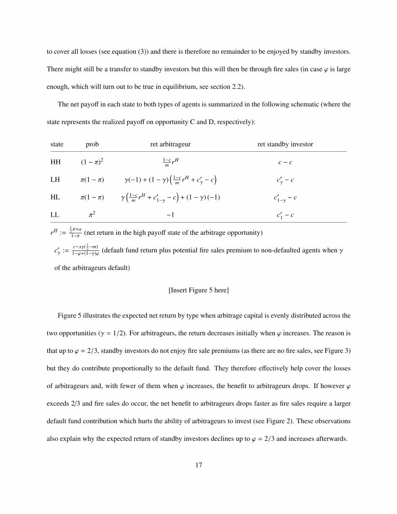
to cover all losses (see equation (3)) and there is therefore no remainder to be enjoyed by standby investors.

There might still be a transfer to standby investors but this will then be through fire sales (in case ϕ is large

enough, which will turn out to be true in equilibrium, see section 2.2).

The net payoff in each state to both types of agents is summarized in the following schematic (where the

state represents the realized payoff on opportunity C and D, respectively):

state prob ret arbitrageur ret standby investor

HH (1 − π)2 1−cm rH c − c

LH π(1 − π) γ(−1) + (1 − γ)(

1−cm rH + c′γ − c

)c′γ − c

HL π(1 − π) γ(

1−cm rH + c′1−γ − c

)+ (1 − γ) (−1) c′1−γ − c

LL π2 −1 c′1 − c

rH :=12π+α

1−π (net return in the high payoff state of the arbitrage opportunity)

c′γ := c−xγ( 12−m)

1−ϕ+(1−γ)ϕ (default fund return plus potential fire sales premium to non-defaulted agents when γ

of the arbitrageurs default)


Figure 5 illustrates the expected net return by type when arbitrage capital is evenly distributed across the

two opportunities (γ = 1/2). For arbitrageurs, the return decreases initially when ϕ increases. The reason is

that up to ϕ = 2/3, standby investors do not enjoy fire sale premiums (as there are no fire sales, see Figure 3)

but they do contribute proportionally to the default fund. They therefore effectively help cover the losses

of arbitrageurs and, with fewer of them when ϕ increases, the benefit to arbitrageurs drops. If however ϕ

exceeds 2/3 and fire sales do occur, the net benefit to arbitrageurs drops faster as fire sales require a larger

default fund contribution which hurts the ability of arbitrageurs to invest (see Figure 2). These observations

also explain why the expected return of standby investors declines up to ϕ = 2/3 and increases afterwards.

17

One salient feature of the arbitrageurs’ expected return is the non-monotonicity in ϕ. For example,

Figure 5 reveals that for most values of ϕ, their return declines in ϕ. But, for a high enough level of ϕ,

the return increases with the proportion of arbitrageurs. The reason is that in the fire-sale region (ϕ>2/3)

there seems to be a net transfer from arbitrageurs to standby investors. The latter benefit disproportionately

from fire sales simply because the arbitrageurs only enjoy fire sale premiums when not in default whereas

standby investors always enjoy them. This net transfer region corresponds to the ϕ interval where the return

to arbitrageurs is strictly negative (as α = 0). For ϕ = 1, however, the arbitrageurs’ return has to equal zero

as there are no standby investors to receive net transfers and the trade economy is a closed system. This

explains why, at some point, the return for arbitrageurs has to increase in ϕ.

The non-monotonicity of arbitrageurs’ expected return in ϕ raises the possibility of multiple equilibria.

Also, the presence of an equilbrium in the example economy does not guarantee its existence in general.

The following proposition states that such equilibrium always exists and is unique.

Proposition 2 (Existence and uniqueness) For each value of trade crowdedness γ, there is a unique value

of ϕ (fraction of arbitrageurs) for which the expected return of an arbitrageurs equals that of a standby

investor.

A key result in the proof is that the expected return of an arbitrageur minus that of a standby investor

monotonically decreases in ϕ. In the fire sale region, beyond some level, both types of agents might benefit

from increased fire sale risk when ϕ increases, but standby investors are shown to benefit more. The intuition

is that there are fewer of them so, per capita, the return to them increases. The proof further shows that the

function is continuous, starts at a strictly positive value for ϕ = 0 and ends at a strictly negative value for

ϕ = 1 (as the return to the last standby investor is infinite; he is, for example, the only one left to cash in

the infinitely large systemic fire sale premium, see discussion below eqn. (3)). The complete proof is in

18

appendix C.


Figure 6 plots the unique equilibrium pairs (ϕ, γ) for a zero expected return and for a positive expected

return on the arbitrage opportunity (α = 0 basis points and α = 3 basis points, respectively). The graph

leads to a couple of observations. First, in equilibrium, the proportion of arbitrageurs (ϕ) is in the fire sale

region for both levels of α. When there is credit risk in the economy because the posted margin is not

sufficient to cover the worst possible loss, fire sales seem to be inevitable. They seem needed as a payoff to

standby investors to generate an expected return that equals that of arbitrageurs. Second, a higher exogenous

return on an arbitrage opportunity (α) increases the fraction of arbitrageurs in equilibrium and, as a result,

lowers overall investment (as the default fund needs to grow in equilibrium). Third, a higher level of trade

crowdedness reduces the fraction of arbitrageurs and increases investment.

These observations can be proven formally and are therefore stated as a corollary.

Corollary 2 (Equilibrium)

1. In a trade economy with credit risk, fire sale risk cannot be eliminated.

2. A higher exogenous return on arbitrage opportunities increases the fraction of agents that become

arbitrageurs and lowers overall investment in the arbitrage opportunities.

3. More crowdedness in trade, i.e., a higher γ, reduces the fraction of agents that become arbitrageurs

and increases overall investment.

A surprising finding is that a higher level of crowdedness reduces investment into the arbitrage opportu-

nities. The key reason is that standby investors benefit from crowdedness and therefore need to earn a lower

fire sales premium. The default fund can therefore be reduced and more capital is available for investment.

19

Is less diversity therefore a better outcome? To answer that question, one needs to set up a social criterion

which requires adding more structure to the economy.

2.3 Decomposition of the expected return by agent type

The expected return for each agent type, arbitrageur and standby investor, can be decomposed into various

components. Define the state as (1C , 1D) where 1i is

1i =

1 if opportunity i hits the low state L,0 otherwise.

(7)

Let l be the fraction of total investment that hits the low state

l := γ1C + (1 − γ)1D. (8)

Denote the survival fraction of arbitrageurs by

ϕ :=ϕ(1 − l)

ϕ(1 − l) + (1 − ϕ)(9)

and the realized CCP loss by

c :=

cPL(portfolio loss)︷︸︸︷lx(

12− m) +

cFS (fire sales)︷︸︸︷lx max

(0,

12−

1 − ϕϕ

). (10)

Expected return arbitrageur. The expected return for arbitrageurs consists of two parts. The return

from investment is

unleveraged payoff︷︸︸︷(1 − c)

((1 − µl) rH + µl

(−

12

))+

additional payoff due to leverage︷︸︸︷(1 − c)(

1m− 1)

((1 − µl)rH + µl

(−

12

))+

limited liability insurance payoff︷︸︸︷(1 − c)

(µl

(2 −

1m

) (−

12

)), (11)

20

where µl is the expected value of l. The expected return from investment simplifies to

(1 − c)((1 − µl)

1m

rH + µl (−1)). (12)

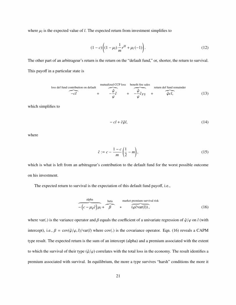
The other part of an arbitrageur’s return is the return on the “default fund,” or, shorter, the return to survival.

This payoff in a particular state is

loss def fund contribution on default︷︸︸︷−cl +

mutualized CCP loss︷︸︸︷−ϕ

ϕc +

benefit fire sales︷︸︸︷−ϕ

ϕcFS +

return def fund remainder︷︸︸︷ϕcl, (13)

which simplifies to

− cl + cϕl, (14)

where

c := c −1 − c

m

(12− m

), (15)

which is what is left from an arbitrageur’s contribution to the default fund for the worst possible outcome

on his investment.

The expected return to survival is the expectation of this default fund payoff, i.e.,

alpha︷︸︸︷−

(c − µϕc

)µl +

beta︷︸︸︷β ∗

market premium survival risk︷︸︸︷(ϕcvar(l)) , (16)

where var(.) is the variance operator and β equals the coefficient of a univariate regression of ϕ/ϕ on l (with

intercept), i.e., β = cov(ϕ/ϕ, l)/var(l) where cov(.) is the covariance operator. Eqn. (16) reveals a CAPM

type result. The expected return is the sum of an intercept (alpha) and a premium associated with the extent

to which the survival of their type (ϕ/ϕ) correlates with the total loss in the economy. The result identifies a

premium associated with survival. In equilibrium, the more a type survives “harsh” conditions the more it

21

benefits from enjoying a fire sale premium and a default fund remainder. The market premium of survival

increases with the fraction of arbitrageurs (ϕ), with what is left of the arbitrageur’s contribution to the fund

on a worst possible outcome on his investment (c), and with the risk of the fraction of investment that hits

the low state (var(l)). A later illustrative example will show that this survival risk premium can become a

substantial part of total return (see section 2.2).

Expected return standby investor. For standby investors the expected return on investment is zero (as

they refrain from investing). Their return on the default fund is similar to eqn. (13)

mutualized CCP loss︷︸︸︷−

(1 − ϕ)1 − ϕ

c +

benefit fire sales︷︸︸︷−

(1 − ϕ)1 − ϕ

cFS +

return def fund remainder︷︸︸︷ϕ

1 − ϕ1 − ϕ

cl, (17)

which yields

ϕ

1 − ϕc(1 − µϕ

)µl + β (ϕcvar(l)) . (18)

where β is the coefficient of a regression of (1 − ϕ)/(1 − ϕ) on l, analogous to the beta of arbitrageurs. It

captures the extent to which survival of the type in the population correlates with the fraction of investment

that hits the low state.

Proposition 3 (Survival risk premium) Part of the expected return for both types of agents, arbitrageurs

and standby investors, is the extent to which their type survives on large aggregate losses in the economy.

Formally, it is

β ∗ λ, (19)

where β is the coefficient of a univariate regression of their proportion among survivors relative to their

ex-ante proportion, on the fraction of investment that hits the low state (l). λ is the market premium of

22

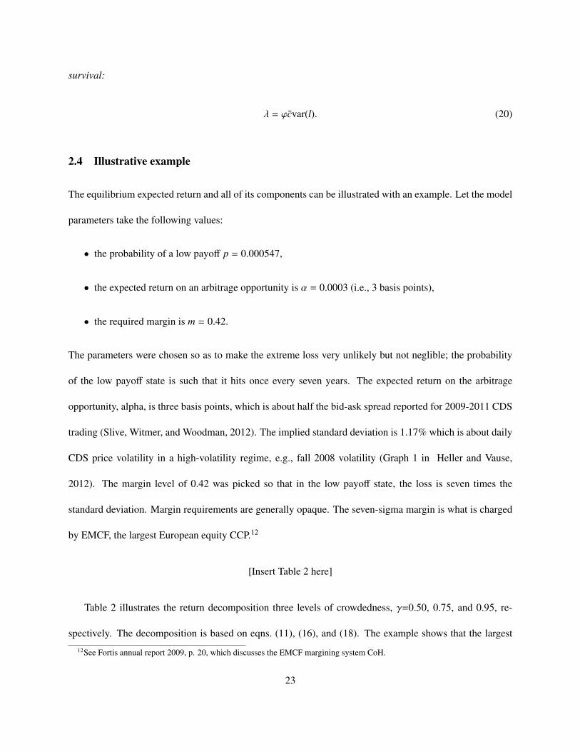
survival:

λ = ϕcvar(l). (20)

2.4 Illustrative example

The equilibrium expected return and all of its components can be illustrated with an example. Let the model

parameters take the following values:

• the probability of a low payoff p = 0.000547,

• the expected return on an arbitrage opportunity is α = 0.0003 (i.e., 3 basis points),

• the required margin is m = 0.42.

The parameters were chosen so as to make the extreme loss very unlikely but not neglible; the probability

of the low payoff state is such that it hits once every seven years. The expected return on the arbitrage

opportunity, alpha, is three basis points, which is about half the bid-ask spread reported for 2009-2011 CDS

trading (Slive, Witmer, and Woodman, 2012). The implied standard deviation is 1.17% which is about daily

CDS price volatility in a high-volatility regime, e.g., fall 2008 volatility (Graph 1 in Heller and Vause,

2012). The margin level of 0.42 was picked so that in the low payoff state, the loss is seven times the

standard deviation. Margin requirements are generally opaque. The seven-sigma margin is what is charged

by EMCF, the largest European equity CCP.12

[Insert Table 2 here]

Table 2 illustrates the return decomposition three levels of crowdedness, γ=0.50, 0.75, and 0.95, re-

spectively. The decomposition is based on eqns. (11), (16), and (18). The example shows that the largest12See Fortis annual report 2009, p. 20, which discusses the EMCF margining system CoH.

23

component of arbitrageurs’ profit on investment is the leverage component. It is about half the return in all

three cases. The limited-liability insurance component is substantial as it is a little over 10% for all levels of

crowdedness.

The survival premium is negative for arbitrageurs, positive for standby investors. Arbitrageurs lose on

their contribution to the default fund irrespective of the fraction of low-state outcomes, and because they

negatively load on this mass and pay the survival risk premium. For perfect diversity (i.e., γ = 1/2, the

two components are -0.80 and -0.20 basis points. Standby investors earn a non-trivial amount on both these

components, 1.83 and 1.43 basis points, respectively. As crowdedness increases, the non-risk component

decreases to 0.98 basis points, whereas the risk premium component increases to 2.62 basis points. It is the

survival risk premium that makes up most of standby investors’ return when trades get crowded. They are

around when most is to be earned in terms of fire sales and a default fund remainder.

3 Welfare

3.1 Welfare in the market for liquidity

Welfare in a trade economy is naturally measured by outside customers’ realized gains from trade.13 One

potential source for such gains is the production of “immediacy” or liquidity by intermediaries as in, for ex-

ample, Grossman and Miller (1988) (see also section 1.2). In their model, Grossman and Miller capture this

market in essentially a two-stage model. In the first stage, outside sellers trade with risk-averse arbitrageurs

(or market makers). These arbitrageurs hold the position through time, incur price risk and, in the second

stage of the game, they sell it to outside buyers. The expected return on the arbitrage opportunity (α) is

endogenous and determined through market clearing in the first stage. All agents are price takers.

13Outside customers are the non-intermediaries. Thus far the analysis was focused only on intermediaries, i.e., arbitrageurs andstandby investors.

24

Welfare as realized gains from trade is calculated from the demand curve of early sellers and the size of

the first-stage trade. It is implicitly assumed that in the second-stage outside buyers do not realize a private

value from trade, only its common value. This stage is admittedly reduced-form as the focus is on early

outside customers who want to trade now; the second-stage trade is best thought off as the “long-term” in

which arbitrageurs can offload a position at fundamental/common value.14 The welfare measure further

ignores the social cost of immediacy production. Such cost is beyond the scope of the current model that

implicitly has a zero-cost assumption embedded for intermediaries.

The demand curve of outside sellers is assumed to be iso-elastic:

p =θ

q1/η , (21)

where η > 0 is the price elasticity of demand. The standard approach to obtain realized customer value is

integrating the demand function from zero to the amount produced, i.e., the quantity traded. This unfortu-

nately cannot be done for relatively inelastic demand (η < 1) as the integral does not exist. It is for this

technical reason that, instead, welfare is measured as realized customer value relative to some, in equilib-

rium, unattainable benchmark level. The technicalities of the construction are included in appendix E. The

interpretation of the proposed welfare measure is the amount by which realized customer value for some

pair (ϕ, γ) falls short of the highest possible (non-equilibrium) level, i.e., (ϕ, γ) = (2/3, 1/2).

The two arbitrage opportunities in the model correspond to two of these markets for immediacy. For

simplicity, they are assumed to be completely orthogonal i.e., outside sellers and buyers are non-overlapping

groups of customers. This polar case of orthogonality serves to keep the focus on the paper’s main topic and

to not burden the analysis with additional notation.

14The model could be extended to create symmetry across the early outside sellers and the late outside buyers. The second-stagetrade would then generate an additional premium for arbitrageurs. It would complicate all mathematical expressions and notationwithout generating additional economic insight.

25

3.2 Diversity and welfare

One intuition is that perfect diversity (γ = 1/2) should yield highest welfare in a trading economy that is

symmetric. Most of the welfare analysis focuses on whether this is generally true. If not, under what condi-

tions is it not true? The strategy is to study how small deviations from diversity affect welfare. This approach

yields an analytic result. Non-local deviations from perfect diversity can only be studied numerically are

therefore charted out in two examples.

The total effect on welfare of a small change (dγ) away from perfect diversity (γ = 1/2) is the sum of a

direct and an indirect effect. The change in welfare can be studied mathematically through a Taylor series

expansion (see appendix E):

dW(ϕ, γ) =

“direct” effect︷︸︸︷W22(dγ)2 +

“indirect” effect︷︸︸︷W11

∂2ϕ

(∂γ)2 (dγ)2 +O((dγ)3

), (22)

where Wi j denotes a partial derivative of the function W to its ith and jth argument respectively. Note that

derivatives W1, W2, W12, and W21 turn out to be zero.15

The small change away from perfect diversity affects welfare through two channels. The first term on

the right-hand side of eqn. (22) is the “direct” effect of a change in diversity, i.e., the effect of ceteris paribus

changing the marginal (liquidity) demander in one market for the marginal demander in the other market.

The second term captures the “indirect” effect, i.e., the equilibrium response to a change in diversity. Such

change affects the expected return of arbitrageurs and standby investors. In equilibrium the proportion of

arbitrageurs (ϕ) has to change to re-establish equality of expected returns across both investor types. This

in turn changes total investment and therefore welfare. The indirect effect can be decomposed into an effect

that operates through the return of any default fund remainder and an effect that operates through alpha, the

15The first-order derivative being zero at γ = 1/2 is not surprising as the economy is symmetric. A small negative change in γshould have the same effect as a small positive change at the point of perfect diversity. The only way this can be true is if that effectis zero.

26

expected return on arbitrage. Both these effects can be signed and lead to the following propositions.

Indirect effect of a diversity change on welfare, default fund channel. A change away from perfect

diversity of investment across the two arbitrage opportunities benefits standby investors over arbitrageurs as

they, in expectation, receive back more of any default fund remainder:

Proposition 4 (Indirect effect, default fund channel) More crowdedness in trade, i.e., a higher γ, implies

that standby investors receive relatively more from any default fund remainder than arbitrageurs, ceteris

paribus.

The default fund remainder channel exists because only non-defaulted agents get a share of what remains

of a default fund. The net effect is non-trivial. First, perfect diversity creates minimum benefit for standby

investors as they have to always share the remains of the default fund with many others in case of a low

payoff on one opportunity and a high payoff on the other; they have to share it with the (1/2)ϕ arbitrageurs

who did not default. The further away one gets from perfect diversity, the fewer others they have to share it

with (i.e., (1 − γ)ϕ) on the low payoff on opportunity C only. The benefit this creates is larger than the cost

of sharing it with more (i.e., γϕ) in the case of a low payoff on opportunity D only.16 Second, a move away

from perfect diversity benefits arbitrageurs as there is less of the default fund available to return to investors

when many arbitrageurs default (as the default fund needs to cover the loss in all trading portfolios). This

happens to be the most likely scenario for an individual arbitrageur who is more likely to end up in the large

group (by construction). The proposition states that the first effect dominates the second effect.

Indirect effect of a diversity change on welfare, arbitrageurs’ alpha channel. A change away from

perfect diversity of investment across the two arbitrage opportunities affects arbitrageurs’ return in the fol-16The reason for this wedge between benefit and cost is that sharing is proportional and the function f (x) = 1/x is convex in the

positive domain. f (x) represents what one would get if one unit has to be shared with x others. Jensen’s inequality says that addinga mean-preserving spread, i.e. a dγ > 0, then generates a higher expected return.

27

lowing way:

Proposition 5 (Indirect effect, alpha channel) More crowdedness in trade, i.e., a higher γ, implies that the

expected return (α) for arbitrageurs

• increases when demand elasticity is less than one (η < 1).

• decreases when demand elasticity is more than one (η > 1).

• remains unchanged when demand elasticity equals one (η = 1).

The expected return for standby investors is unaffected.

The intuition for this proposition is that less diversity has two effects on the expected return on arbitrage.

First, the premium increase in the deserted opportunity is larger than the premium decrease in the crowded

one. The reason is that the demand curves are convex, i.e., the marginal utility for one more unit of “immedi-

acy” is decreasing in immediacy production. This effect raises the expected return. Second, the probability

that an individual arbitrageur invests in the deserted opportunity is reduced as, by construction, fewer ar-

bitrageurs end up investing in this opportunity. This effect reduces the expected return. The first effect

strengthens when demand becomes less elastic (demanders care less about price when determining their

consumption) whereas elasticity has no bearing on the second effect. Less elastic demand therefore raises

arbitrageurs’ expected return.

Net effect of a diversity change on welfare. The effect on welfare of a change in diversity cannot be

signed in general. The direct effect is negative, but it could be compensated by the indirect effect which has

the potential to be positive. More could be invested into arbitrage in equilibrium if less diversity leads to

fewer arbitrageurs (cf. Corollary 1). This happens when the return to standby investors is raised relative to

that of arbitrageurs on a change in diversity. Proposition 1 states that there is a raise in expected return for

28

standby investors. Proposition 5 states that expected return for arbitrageurs depends on demand elasticity. It

is negative for inelastic demand and positive for elastic demand. This demand elasticity result turns out to

be powerful as it can push the indirect effect in such a way that it can dominate the direct effect and produce

a positive welfare result on a change away from perfect diversity.

Proposition 6 (Welfare and perfect diversity) The effect on welfare of more crowdedness in trade, i.e., a

higher γ, cannot be signed.

The proposition is “proven” in the next section by providing two examples.

3.3 Illustration of the welfare effect

This section illustrates the welfare effect through an analysis of an inelastic and an elastic demand example.

The example extends the baseline example of section 2.4 by endogenizing alpha. The inelastic demand

example shows that a change away from perfect diversity can reduce welfare. The elastic demand example

shows the opposite result, i.e., a change away from perfect diversity can raise welfare.

The price elasticities of demand considered here are η = 1/2 and η = 5. The scaling parameter θ in

the liquidity demand function is set such that the expected return on investment in equilibrium on perfect

diversity (αθ is 0.0003 (equal to the exogenous α in the baseline example). The elasticities were chosen

somewhat arbitrarily as there is no evidence available for the CDS market. Empirical studies for equities

suggest prices elasticities of five or higher (Hollifield et al., 2006; Hendershott and Menkveld, 2014).

[Insert Table 3 and Figure 7 here]

Example inelastic demand. The contour plot in Panel A of Figure 7 illustrates how welfare for a rel-

atively inelastic liquidity demand (η = 1/2) varies with the fraction of arbitrageurs (ϕ) and the level of

29

crowdedness (γ). The “horizontal” pattern in the graph follows directly from how total investment into the

arbitrage opportunities varies with the fraction of arbitrageurs (see Panel B of Figure 2). The vertical pattern

is not surprising as perfect diversity should yield highest welfare. Any deviation will swap higher marginal

utility sellers from one market with lower marginal utility sellers in the other market. This is the result of a

downward-sloping demand curve in both markets.

Panel B of Figure 7 illustrates that less diversity can reduce welfare. The iso-welfare curves seem to be

exhibit more curvature than the solid line that represents equilibrium (ϕ, γ) pairs. A move away from perfect

diversity therefore appears to reduce welfare.

Table 3 decomposes the effect a small change from perfect diversity has on welfare (analytic result). The

total effect of a small change in γ away from γ = 1/2, say dγ = 1/10, reduces welfare by approximately

1483 ∗ (1/10)2 = 14.83%. This total effect is the sum of a direct effect of -15.98% and an indirect effect of

1.16%. This is consistent with Panel B of Figure 7 as the change in the equilibrium ϕ on a change in γ is

very small relative to the change in welfare on a change in γ. The indirect effect of 1.16% can be further

decomposed into a 4.12% welfare increase due to the default fund channel (cf. Proposition 4) and a welfare

decrease of 2.96% due to an increase in arbitrageurs’ return (cf. Proposition 5).


Example elastic demand. A higher level of crowding can raise welfare when demand is elastic. For

the relatively inelastic demand case analyzed in Figure 7, welfare decreased on a small change away from

perfect diversity. Figure 8 replots the graph of this figure for a demand elasticity of η = 5 instead of η = 1/2.

This time welfare is increased when leaving the perfect diversity case; the equilibrium (ϕ, γ) line exhibits

more curvature than the iso-welfare curves. In fact, there seems to be an optimum level of crowdedness at

about 80%.

30

Table 3 reports the size of the welfare increase and, more importantly, its sources. A change in γ of 1/10

increases welfare by 0.42%. This differs markedly from the -14.83% in the inelastic demand case. One of the

two components that makes welfare increase is the direct effect, which is raised from −15.98% to −0.40%.

The reason is that more elastic demand implies less variation in the marginal value of immediacy among

outside sellers. The effect on welfare of swapping, ceteris paribus, an outside seller from one market for

one in the other market therefore becomes smaller. The other component that raises welfare is the indirect

effect through a change in the return on arbitrage (α) which changes welfare from −2.96% to 0.04%. This is

essentially the result of Proposition 5; arbitrageurs’ expected return is negative on inelastic demand (η < 1)

and positive on elastic demand (η > 1). This implies that in equilibrium there are fewer arbitrageurs, the

default fund can therefore be reduced and this, in turn, frees up more of the agents’ capital for investment.

The indirect effect through the default fund channel is reduced from 4.12% to 0.77%. This is the result of

welfare being less responsive to total investment when demand is elastic.17

4 Further discussion

All agents are risk-neutral and a diversification motivation for spreading wealth across the two opportunities

is therefore absent. If this additional motivation were present it is likely that there is a level of risk aver-

sion beyond which arbitrageurs prefer diversification over betting all their money on a single risk factor as

predicted by Proposition 1. The “diversification-diversity” tradeoff is beyond the scope of this study, but is

analyzed thoroughly in Wagner (2011).

All agents contribute an equal amount to the default fund ex-ante. This is an extreme simplification as,

in practice, historical trade portfolio risk is taken into account when calculating contributions (Zhu, 2011,

17The partial derivative of the equilibrium ϕ to γ due to the default fund channel does not depend on the shape of the demandcurve; it is entirely driven by the relative advantage standby investors have when there is less than perfect diversity. This effect isvisible in the exogenous-α curves in Figures 6, 7 and 8. These curves are all the same. The difference in the effect on welfare issolely due to a multiplication with the partial derivative of welfare to ϕ which does depend on the shape of the demand function.

31

p. 51-52). The model could be adjusted to have standby investors contribute less to the fund ex-ante. The

equilibrium proportion of arbitrageurs is expected to be lower as some will change type to benefit from

the lower contribution until equality in expected return is restored. The model’s main trade-offs remain

unchanged.

Survivors share proportionally in fire sales and in a potential default fund remainder. Could the CCP not

distribute a larger share ex-post to standby investors in order to reduce “overinvestment” by arbitrageurs?

This would reduce the limited-liability externality. Such procedure would be hard to implement in reality.

It would involve ex-post identification of arbitrage activity. In the model, it would be those who invested

in arbitrage and survived. Their counterpart in reality would be those who traded large and risky trade

portfolios, and survived. A natural reply of these agents would be that they survived because of the large

trade portfolio, i.e., they actively hedged. One would not want to discourage such behavior. It seems

proportional sharing is the only implementable solution. Moreover, proportional sharing seems appropriate

as the static model is an approximation of reality where, going forward, any burden or windfall in the default

fund is shared proportionately by all contributors.

5 Conclusion

This paper proposes a model for centralized clearing focused on systemic liquidation risk due to default

of arbitrageurs. Endogenously, some in the population of candidate arbitrageurs become standby investors,

i.e., they refrain from investing into arbitrage opportunities. Instead, they earn a fire sale premium in case a

CCP needs to resell a position inherited from arbitrageurs in default and, if available, share any default fund

remainder with all non-defaulted agents. The size of the default fund maintained by the CCP is endogenous

and pinned down by an obligation to cover trade losses and fire sale premiums in all states of the world. It

depends on the extent to which arbitrageurs crowd in the same trade opportunity.

32

The net effect on welfare of steering arbitrageurs away from crowded trades is non-trivial. Perfect diver-

sity is good in the sense that a balanced spread of capital across arbitrage opportunities equally benefits all

liquidity demanders who are the source of the opportunity (Grossman and Miller, 1988). Perfect diversity

is bad in the sense that it reduces the expected return for standby investors. In equilibrium, more diversity

implies that their mass shrinks, fire sale premiums go up, and with it also the size of the default fund. It ap-

pears that this cost of diversity dominates its benefit when liquidity demand at the source of the opportunity

is price elastic. Hollifield et al. (2006) empirically document a relatively high price elasticity of demand,

which implies that some level of crowding in trades is socially optimal.

Appendix

A Regulation

This appendix contains quotes from two recent regulatory documents that emerged from cooperative effort of

the Bank for International Settlements (BIS) and the International Organization of Securities Commissions

(IOSCO). The first document, BIS-IOSCO (2004), contains recommendations for central counterparties.

The second document, BIS-IOSCO (2012), takes an integrative approach and embeds CCP recommmenda-

tions into more general recommendations for “financial market infrastructures.” The document emphasizes

systemic risk. Emphasis was added to parts of the quotes as they speak to the model proposed in this paper.

In their review of a CCP’s risks and risk management BIS-IOSCO (2004, p. 11) writes the following

about financial resources:

“Participation requirements, position limits and the margin system represent a package of tech-

niques available to a CCP to mitigate credit and liquidity risks. While they provide substantial

protection to a CCP, losses in the event of a participant’s default might exceed the resources of

33

that participant on which a CCP has a claim, for several reasons. Margin requirements cover

a high percentage of likely price movements, but they are not set at a level that is intended

to cover all price movements (particularly movements in the tails of distributions of probable

price changes). More time might elapse before a CCP can liquidate a defaulting participant’s

positions (for instance because of illiquid markets) than was assumed in the design of the risk

management tools. Furthermore, a defaulting participant may have increased its positions since

the last settlement.

CCPs thus maintain resources to provide protection against exposures not covered by a default-

ing participant’s assets and to provide liquidity while realising the proceeds of those assets.

These resources, together with the risk management tools, determine the overall level of pro-

tection provided by the system and how risks and costs are shared among the stakeholders of a

CCP. Some CCPs hold a blended pool of resources, often called a clearing fund, which is in-

tended to cover both a large proportion of likely exposures and exposures resulting from more

unusual market conditions.”

In their recommendation 5 that pertains to financial resources, BIS-IOSCO (2004, p. 23) states18:

“Although risk management tools (notably a CCP’s participation requirements) are designed

to ensure that defaults are unlikely, a CCP should nonetheless plan for the possibility of a

default occurring. In that event, a CCP has an obligation to continue to make payments to non-

defaulting participants on time. It should maintain financial resources both to provide it with

liquidity to make timely payments in the short term and to enable it to cover the losses that

result from defaults.

18The European Central Bank (ECB) and the Committee of European Securities Regulator (CESR) largely followed these rec-ommendations in their 2009 report (ECB-CESR, 2009).

34

Assessing the adequacy of resources can be difficult because it rests on assumptions about

which participant or participants default and about market conditions at the time of the default.

Many CCPs focus on a default by the participant to which the CCP has the largest exposure

in the market scenarios under consideration. This should be viewed as a minimum standard

in a CCP’s evaluation of its resources. However, market conditions that typically accompany

a default put pressures on other participants (particularly related group members or affiliates),

and a default itself tends to heighten market volatility, further contributing to stresses. Planning

by a CCP should consider the potential for two or more participants to default in a short time

frame, resulting in a combined exposure greater than the single largest exposure.”

In the wake of the financial crisis, BIS-IOSCO (2012) focuses on entire financial market infrastructures

(FMIs) that includes CCPs as well as, for example, payment systems (PSs), central security depositories

(CSDs), securities settlement systems (SSSs), or trade repositories (TRs). The list of risks is largely similar

to their earlier report, except for systemic risk which tops the list. In its discussion of systemic risk it

identifies “knock-on”’ effects due to the inability of a participant to deliver on his “promise.” An example

of such effect is the immediar liquididation of collateral, margin, or other assets at fire sale prices. It further

emphasizes complex interdependencies that may be a normal part of an FMI and its operations (p. 18).

In a later chapter the report discusses the margins a CCP imposes. It emphasizes that they cover liqui-

dation cost as a net trade portfolio of a member in default needs to be unwound in a “close-out period:”

“The close-out period should account for the impact of a participant’s default on prevailing

market conditions. [...] A CCP should also consider and address position concentrations, which

can lengthen close-out timeframes and add to price volatility during close outs.”

35

B Notation summary

α expected net return arbitrage opportunity

γ fraction of arbitrageurs who invest in arbitrage opportunity 1; (1-γ) is the fraction of arbitrageurs who

invest in opportunity 2

ϕ fraction of agents who become arbitrageur; (1-ϕ) is the fraction of agents who become standby in-

vestors

c the default fund tax rate that is ex-ante levied on all agents; it also denotes the size of the default fund

as there is a unit mass of agents

m margin, i.e., the down payment as a fraction of the total amount invested

π probability of the low payoff on an investment opportunity

x the total amount invested

C Proofs

Proof of Proposition 1. Suppose the investor chose to invest δx/ϕ in one opportunity and (1 − δ)x/ϕ

in the other, δ ∈ [0, 1]. Note that x/ϕ is the maximum amount an investor can invest (and will invest by

assumption). Denote the independent and identically distributed random payoffs on the two opportunities

by ri (for the argument it does not matter which is C and which is D). The expected return on investment is

E(max

(δ

xϕ

r1 + (1 − δ)xϕ

r2, 0)). (A1)

As the max(., 0) function is convex, Jensen’s inequality immediately yields that adding a mean-preserving

spread raises the expected value of the function. It strictly raises the expected value when the domain of

the distribution contains both strictly negative and strictly positive values. The expected value is therefore

maximized at the extremes, i.e., δ=0 or δ=1.

36

The assumption in the primitives that arbitrageurs maximize investment can be dropped in equilibrium

where the expected return for standby investors equals the expected return of fully-invested arbitrageurs. Ar-

bitrageurs will now endogenously choose to stay fully-invested. The reason is that any amount not invested

will yield the same expected return (i.e., that of a standby investor), but it strictly reduces overall return

volatility and when taken into the function max(., 0) reduces overall expected return (Jensen’s inequality

again).19

Proof of Proposition 2. Rearranging terms yields:

A earns an expected excess ret on arb opp︷︸︸︷(1 − π)

(1 − cϕ

m

) 12π + α

1 − π

−

︷︸︸︷π(1 − cϕ

)A loses contrib DF

=

=

︷︸︸︷π (1 − π)

(1 − γ)cϕ − xϕ(1 − γ)

(12 − m

)1 − ϕ + γϕ

+ γcϕ − xϕγ

(12 − m

)1 − ϕ + (1 − γ)ϕ

S earns a relative benefit on fire sales and return of default fund remainder

+

︷︸︸︷π2

cϕ − xϕ(

12 − m

)1 − ϕ

S earns systemic fire sales premium

(A2)

Note that both xϕ and cϕ are functions of ϕ (see eqns. .(2) and (3) respectively). The left-hand-side

could be interpreted the excess return to being an arbitrageur i.e., one earns the alpha associated with the

arbitrage opportunity, but one loses the contribution to the default fund on a negative shock. The right-hand-

side represents the excess return to standby investors who benefit from potential fire sales and a default

fund payout when only one arbitrage opportunity goes sour and earn the “jackpot” when both arbitrage

opportunities fail, i.e., they earn the systemic fire sale premium.

Proof of Proposition 5. The expected return for arbitrageurs is:

α(γ; n) = γθ(

γxϕ)n + (1 − γ)

θ((1 − γ) xϕ

)n . (A3)

19The returns of arbitrageurs and standby investors are negatively correlated given that the trade economy is a closed system.

37

Its partial derivative with respect to γ is:

∂α

∂γ= θ (n − 1) x−n

ϕ

((1 − γ)−n − γ−n) . (A4)

The sign of this derivative is determined by the sign of (1 − n) for γ > 1/2. The same is true for γ < 1/2.

The result of the proposition follows immediately.

D Sketch of a model with trade-based margins

The alternative economy extends the baseline economy with an option for the CCP to steer traffic through

trade-based margins. Should one arbitrage opportunity get too crowded (and the CCP is the only one to

observe), then it could raise the margin on the opportunity to steer further traffic away. To study the relative

merit of such trade-based margins, the economy investment stage might altered as follows:

Preparation stage (alternative model).

1 The CCP collects a tax c from all agents to create a default fund of size c (as there is a unit mass of

agents) announces that it will use trade-based margins to stop arbitrageurs to invest more in an oppor-

tunity when it reaches a crowdedness limit, say γ. The CCP has a commitment device (e.g. reputation

or regulatory oversight) to ensure that it does ex-post (in step 3, see below) what it announces ex-ante.

Investment stage (alternative model).

3 a) The CCP communicates mi = (mi1,mi2) to investor i at the time of his arrival, where mi j ∈ {m,∞}.20

The CCP keeps the margin mi at m initially but raises it to infinity as soon as an opportunity reaches

the upper bound γ.

20This set is extremely narrow to ensure that the level of credit is not altered relative to the baseline economy; m is fixed at anexogenous level throughout. The only option a CCP gets is to stop traffic completely by raising the margin to infinity. In reality aCCP will have a continuum of margin levels at its disposal.

38

b) Investors are picked randomly from the set of investors that have not yet arrived. On arrival, the ith

investor observes mi and decides to invest in 1 or 2. Continue to step 4 if all arbitrageurs have arrived,

otherwise return to a).

To construct an equilibrium one would need to specify an exogenous distribution over the probability that

arbitrageurs pick opportunity C, say X ∼ F(X) with X ∈ [1/2, 1] almost surely. The upperbound γ implies

that intermediaries (arbitrageurs and standby investors) should expect the following ex-post distribution for

γ:

g(x) =

f (x) for 1/2 ≤ x < γ,1 − F(γ) for x=γ,

0 otherwise.

(A5)

The expected return for arbitrageurs and standby investors in the baseline model depend on an exoge-

nously given γ. The expected returns in the alternative economy would take the expectation of these expected

returns with respect to γ. Equilibrium can then again be defined as those (ϕ, γ) pairs for which the expected

return of arbitrageurs equals that of standby investors. The analysis becomes an order of magnitude more

complex due to the additional expectation with respect to γ and is unlikely to yield analytic results. The

baseline economy developed in the main text is a first step in the direction of such candidate alternative

model. Its advantage is that it can be characterized analytically for γ = 1/2.

E Other results

Welfare. The welfare measure is constructed based on realized liquidity demand. Standard integration of

the demand function (eqn. (21)) from zero to realized demand is not always possible as the integral might

be unbounded (for inelastic demand functions, i.e., n < 1). To avoid degenerate integrals, welfare is defined

39

relative a demand level that is impossible to attain.21

The benchmark demand level is fixed at four units that are evenly spread across the two markets. This

four-unit benchmark level is out of reach as it would obtain if all agents become arbitrageur, invest their

entire one unit of wealth and are able to leverage it one to four as the default margin requirement, m = 1/4.

It is implicitly assumed that no tax needs to be paid to fill the default fund. And, no agent is left to standby

when on a bad draw on the payoff function. Finally, the downward-sloping demand curve ensures that a n

even spread across the two arbitrage opportunities generates highest welfare. These observation imply that

this benchmark demand level is indeed out of reach.

The welfare distance for a (ϕ, γ) pair is:

D(ϕ, γ) =

∫ 2

γxϕ

θ

q1/n dq +

∫ 2

(1−γ)xϕ

θ

q1/n dq = θ1

1 − 1n

(2 ∗ 21− 1

n −(γxϕ

)1− 1n−

((1 − γ)xϕ

)1− 1n

). (A6)

The welfare measure is the distance for (ϕ, γ) relative to the minimum distance that could be achieved, i.e.,

(ϕ, γ) = (2/3, 1/2):

W(ϕ, γ) =D(ϕ, γ) − D( 2

3 ,12 )

D( 23 ,

12 )

. (A7)

References

Acharya, Viral V. 2009. “A Theory of Systemic Risk and Design of Prudential Bank Regulation.” Journalof Financial Stability 5:224–255.

Acharya, Viral V. and Alberto Bisin. 2011. “Counterparty Risk Externality: Centralized versus Over-the-Counter Markets.” Manuscript, NYU.

Allen, Franklin and Douglas Gale. 1994. “Limited Participation and Volatility of Asset Prices.” AmericanEconomic Review 84:933–955.

Amini, Hamed, Damir Filipovic, and Andreea Minca. 2014. “Systemic Risk and Central CounterpartyClearing.” Manuscript, EPFL, Lausanne.

21The difference between two integrals that might each tend to infinity might become finite:∫ b

0f (q)dq−

∫ a

0f (q)dq =

∫ b

af (q)dq.

40

Basak, Suleyman and Alexander Shapiro. 2001. “Value-at-Risk-Based Risk Management: Optimal Policiesand Asset Prices.” Review of Financial Studies 14:371–405.

BCBS and IOSCO. 2013. “Margin Requirements for Non-Centrally Cleared Derivatives.” Manuscript,Basel Committee on Banking Supervision (BCBS) and the Board of the International Organization ofSecurities Commissions (IOSCO).

Bernanke, Ben S. 2011. “Clearinghouses, Financial Stability, and Financial Reform.” Speech, FED.

Biais, Bruno, Florian Heider, and Marie Hoerova. 2011. “Clearing, Counterparty Risk, and Aggregate Risk.”Manuscript, IMF.

BIS-IOSCO. 2004. “Recommendations for Central Counterparties.” Manuscript, Bank for InternationalSettlements and International Organization of Securities Commissions.

———. 2012. “Principles for Financial Market Infrastructures.” Manuscript, Bank for International Settle-ments and International Organization of Securities Commissions.

———. 2014. “Recovery of Financial Market Infrastructures.” Manuscript, Bank for International Settle-ments and International Organization of Securities Commissions.

Cumming, Fergus and Joseph Noss. 2013. “Assessing the Adequacy of CCPs’ Default Resources.”Manuscript, Bank of England.

Duffie, Darrell. 2010a. How Big Banks Fail and What to Do about It. Princeton: Princeton University Press.

———. 2010b. “Presidential Address: Asset Price Dynamics with Slow-Moving Capital.” Journal ofFinance 65:1237–1267.

———. 2014. “Financial Market Infrastructure: Too Important to Fail.” In The U.S. Financial System –Five Years After the Crisis, edited by Martin Bailey and John Taylor. Washington DC: Hoover Institutionand Brookings Institute.

ECB-CESR. 2009. “Recommendations for Securities Settlement Systems and Recommendations for Cen-tral Counterparties in the European Union.” Manuscript, European Central Bank and the Committee ofEuropean Securities Regulator.

ESMA. 2012. “European Market Infrastructure Regulation.” Manuscript, European Securities and MarketsAuthority.

EU. 2013. “Regulatory Technical Standards on Requirements for Central Counterparties.” Manuscript,153/2013.

Farhi, Emmanuel and Jean Tirole. 2012. “Collective Moral Hazard, Maturity Mismatch, and SystemicBailouts.” American Economic Review (forthcoming) .

Fontaine, Jean Sébastien, Hector Perez-Saiz, and Joshua Slive. 2014. “How Should Central CounterpartyClearing Reduce Risk? Collateral Requirements and Entry Restrictions.” Manuscript, Bank of Canada.

Freixas, Xavier and Bruno Parigi. 1998. “Contagion and Efficiency in Gross and Net Interbank PaymentSystems.” Journal of Financial Intermediation 7:3–31.

41

Galai, Dan and Ronald W. Masulis. 1976. “The Option Pricing Model and the Risk Factor of Stock.” Journalof Financial Economics 3:53–81.

Grossman, Sanford J. and Merton H. Miller. 1988. “Liquidity and Market Structure.” Journal of Finance43:617–633.

Hedegaard, Esben. 2012. “How Margins are Set and Affect Prices.” Manuscript, NYU.

Heller, Daniel and Nicholas Vause. 2012. “Collateral Requirements for mandatory Central Clearing ofOver-the-Counter Derivatives.” Manuscript, Bank for International Settlements.

Hendershott, Terrence and Albert J. Menkveld. 2014. “Price Pressures.” Journal of Financial Economics(forthcoming).

Hendershott, Terrence and Mark S. Seasholes. 2007. “Market Maker Inventories and Stock Prices.” Ameri-can Economic Review 97:210–214.

Hollifield, Burton, Robert A. Miller, Patrik Sandås, and Joshua Slive. 2006. “Estimating the Gains fromTrade in Limit Order Markets.” Journal of Finance 61:2753–2804.

Jensen, Michael C. and William H. Meckling. 1976. “Theory of the Firm: Managerial Behavior, AgencyCosts and Ownership Structure.” Journal of Financial Economics 3:305–360.

Jones, Robert A. and Christophe Pérignon. 2013. “Derivatives Clearing, Default Risk, and Insurance.”Journal of Risk and Insurance 80:373–400.

Khandani, Amir E. and Andrew W. Lo. 2007. “What Happened to the Quants in August 2007?” Journal ofInvestment Management 5:5–54.

Koeppl, Thorsten, Cyril Monnet, and Ted Temzelides. 2012. “Optimal Clearing Arrangements for FinancialTrades.” Journal of Financial Economics 103:189–203.

Koeppl, Thorsten V. and Cyril Monnet. 2014. “The Emergence and Future of Central Counterparties.”Manuscript, Queen’s University.

Loon, Yee Cheng and Zhaodong Ken Zhong. 2014. “The impact of central clearing on counterparty risk,liquidity, and trading: Evidence from the credit default swap market.” Journal of Financial Economics112:91–115.

Cruz Lopez, Jorge A., Jeffrey H. Harris, Christophe Hurlin, and Christophe Pérignon. 2014. “CoMargin: ASystem to Enhance Financial Stability.” Manuscript, HEC Paris.

Menkveld, Albert J. 2014. “Crowded Trades: An Overlooked Systemic Risk for Central Clearing Counter-parties.” Manuscript, VU University Amsterdam.

Menkveld, Albert J., Emiliano Pagnotta, and Marius A. Zoican. 2013. “Clearing and Asset Prices.”Manuscript, NYU.

Nahai-Williamson, Paul, Tomohiro Ota, Mathieu Vital, and Anne Wetherilt. 2013. “Central Counterpartiesand Their Financial Resources – A Numerical Approach.” Manuscript, Bank of England.

42

Rochet, Jean-Charles and Jean Tirole. 1996. “Interbank Lending and Systemic Risk.” Journal of Money,Credit, and Banking 28:733–762.

Slive, Joshua, Jonathan Witmer, and Elizabeth Woodman. 2012. “Liquidity and Central Clearing: Evidencefrom the CDS Market.” Manuscript, Bank of Canada.

Stein, Jeremy C. 2009. “Presidential Address: Sophisticated Investors and Market Efficiency.” Journal ofFinance 64:1517–1548.

Wagner, Wolf. 2011. “Systemic Liquidation Risk and the Diversity-Diversification Trade-Off.” Journal ofFinance 66:1141–1175.

Zhu, Siyi. 2011. “Is There a “Race to the Bottom” in Central Counterparties Competition?” Manuscript,De Nederlandsche Bank Occasional Studies 9/6.

43

Table 1: Credit default swap (CDS) positions of 14 main derivatives dealers

This table presents the 2010 net position in credit default swaps (CDS) of the fourteen main derivativesdealers, known as the G14. It disaggregates net position (i.e., protection bought minus protection the totalprotection sold) by the G14 across continent, security security class (MN: multi-name, SN: single-name),and industry.

CDS net position G14, by contract type, 2010

($ billion) Americas Europe Asia None TotalMN: corporate -19 -37 -3 1 -58MN: government 0 -8 0 0 -8MN: other -4 0 0 0 -4SN: basic materials -4 -5 -1 0 -10SN: consumer goods -9 -7 -1 0 -17SN: consumer services -13 -10 -1 0 -24SN: financials -19 -16 -3 0 -38SN: government -6 -16 -4 0 -26SN: health care -3 -1 0 0 -4SN: industrials -6 -6 -1 0 -13SN: oil & gas -5 -2 0 0 -7SN: technology/telecoms -5 -8 -2 0 -15SN: utilities -3 -6 0 0 -9SN: other 0 0 0 -7 -7Total -96 -122 -16 -6 -240

Source: Heller and Vause (2012, Table 6)

44

Table 2: Agent return decomposition, a CAPM type result

This table decomposes the expected return for both types of agents: arbitrageurs and standby investors.These returns are equilibrium returns for a low, medium, and a high level of crowdedness (γ=0.5, 0.75, and0.9, respectively). A first decomposition is according to the net return on investment versus the net returnon survival (to cash in on CCP fire sales and the default fund remainder). The investment return is furtherdecomposed into: an unleveraged return (which falls short of 3 basis points as part of an agent’s wealthis taxed to fill the default fund ex-ante); an additional return due to leverage (the margin m is 0.42); anda return due to limited-liability insurance. The survival return component is further decomposed into anoverall average and a component that is due to the extent to which an agent type survives (relative to theother type) correlates with the fraction of investment that hits the low state. Formally, this is the beta of aregression of the relative survival fraction of the agent type on the fraction of investment that hits the lowstate. A high beta implies that the agent type can cash in more on a premium associated with fire sales anda potential default fund remainder. The table further reports the equilibrium proportion of arbitrageurs ϕ∗.

Panel A: Agent return decompositionpayoffs (bps) arbitrageur standby investor

trade crowdedness trade crowdednesslow med high low med high

γ=.50 γ=.75 γ=.95 γ=.50 γ=.75 γ=.95investment alpha unleveraged 1.56 1.71 1.94 0 0 0

alpha leverage 2.16 2.36 2.68 0 0 0alpha lim liability insurance 0.54 0.59 0.67 0 0 0total 4.26 4.67 5.30 0 0 0

survival alpha survival -0.80 -0.89 -0.95 1.83 1.47 0.98survival premium, β ∗ λ -0.20 -0.39 -0.75 1.43 1.93 2.62total -1.00 -1.27 -1.70 3.26 3.39 3.60

total 3.26 3.39 3.60 3.26 3.39 3.60

Panel B: Survival premium decompositionsurvival beta survival, β -0.22 -0.42 -0.85 1.57 2.11 2.97

market premium survival, λ 0.91 0.91 0.88 0.91 0.91 0.88

Panel C: Equilbrium proportion arbitrageurs (ϕ∗)ϕ∗ 0.88 0.83 0.78 0.88 0.83 0.78

45

Table 3: Effect on welfare of a change away from perfect diversity

This table illustrates how welfare changes when arbitrageurs’ capital is steered away from perfect diversity,i.e., the two symmetric markets for liquidity get receive investment from arbitrageurs (γ = 1/2). Welfareis measured by realized liquidity demand aggregated across the two markets. The arbitrageurs’ expectedreturn (α) is equal to the liquidity premium that is endogenously generated in these markets for liquidity (c.f.Grossman and Miller (1988)). The effect of a small change to diversity (∂γ) on welfare is (see appendix):

dW(ϕ, γ) =

“direct” effect︷︸︸︷W22(dγ)2 +

“indirect” effect︷︸︸︷W11

∂2ϕ

(∂γ)2 (dγ)2 +O((dγ)3

)where Wi j denotes a partial derivative of the function W first to its ith argument and then to its jth argument.The first term is the “direct” effect of a change in diversity, i.e., the effect of changing the marginal (liq-uidity) demander in one market for the marginal demander in the other keeping total investment fixed. The“indirect” effect is the equilibrium response to a change in diversity. Such change affects the expected returnof arbitrageurs and standby investors. This implies a shift in the proportion of arbitrageurs and therefore achange in total investment which in turn affects welfare. The table presents the size of the total effect ofa diversity change on welfare and decomposes it into the direct effect and both components of the indirecteffect. The size of these effects is presents for low and high price elasticity of demand and therefore corre-spond to Figure 7 and 8. The interpretation of the numbers is that, for example, a diversity change of tenpercentage points reduces welfare by approximately 1483 ∗ (1/10)2 = 14.83 percentage points.

effect of small change away from perfect diversity on welfare

demandelasticity direct

indirect,throughchangedefaultfundreturn

indirect,throughchangeinarbitragereturn

indirect,total

total,direct+

indirect

low, 1/2 -1598 412 -296 116 -1483high, 5 -40 77 4 81 42

46

Figure 1: Initial margin G14 CDS portfolios

Heller and Vause (2012) estimate what the initial margin requirement would have been on the 2010 CDSportfolio positions on the main 14 derivatives dealers, the G14. The graph below was taken from theirreport and presents the outcome for a low, medium, and high volatility period (June 2006, March 2008, andOctober 2008, respectively).

Source: Heller and Vause (2012, Graph 11)

47

Figure 2: Default fund tax and overall investment

Panel A graphs the (minimum) tax a CCP has to charge all agents in order to fill its default fund to thelevel where it remains solvent in all states of the world. It is equal to the default fund size as there is a unitmass of agents in the economy. Panel B graphs total investment by the arbitrageurs invested into arbitrageopportunities. The margin m equals 0.42.

Panel A: Ex-ante tax levied on all agents to fill the default fund

0.0 0.2 0.4 0.6 0.8 1.0proportion of arbitrageurs (φ)

0%

10%

20%

30%

40%

50%

60%

70%

fire sales boundary

tax to fill default fund

48

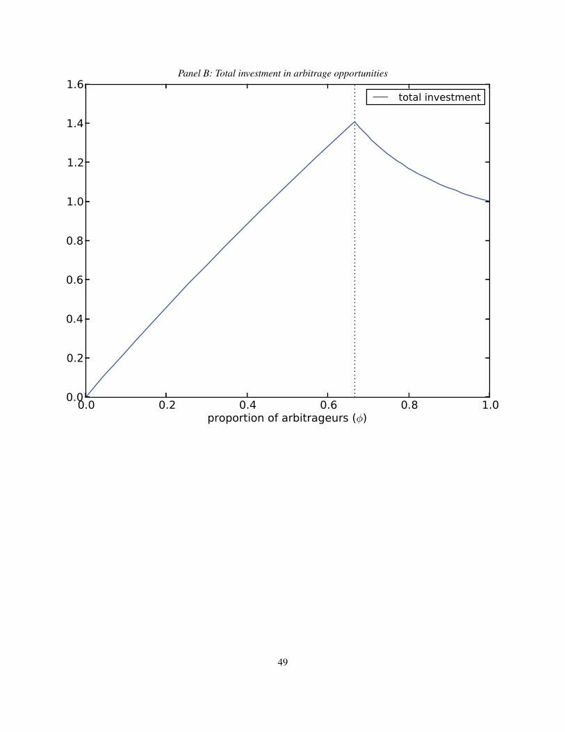
Panel B: Total investment in arbitrage opportunities


0.0

0.2

0.4

0.6

0.8

1.0

1.2

1.4

1.6total investment

49

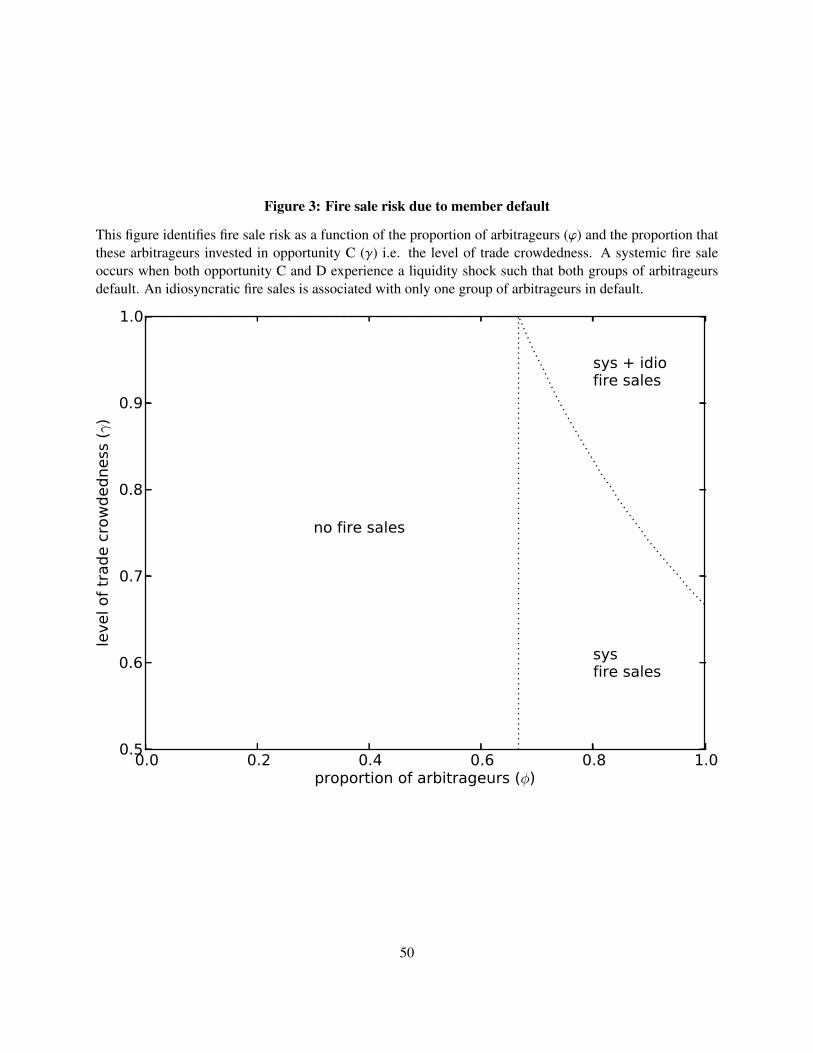
Figure 3: Fire sale risk due to member default

This figure identifies fire sale risk as a function of the proportion of arbitrageurs (ϕ) and the proportion thatthese arbitrageurs invested in opportunity C (γ) i.e. the level of trade crowdedness. A systemic fire saleoccurs when both opportunity C and D experience a liquidity shock such that both groups of arbitrageursdefault. An idiosyncratic fire sales is associated with only one group of arbitrageurs in default.


0.5

0.6

0.7

0.8

0.9

1.0

level of

trade c

row

dedness

(γ)

sys + idiofire sales

sysfire sales

no fire sales

50

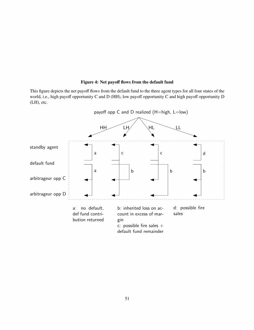
Figure 4: Net payoff flows from the default fund

This figure depicts the net payoff flows from the default fund to the three agent types for all four states of theworld, i.e., high payoff opportunity C and D (HH), low payoff opportunity C and high payoff opportunity D(LH), etc.

payoff opp C and D realized (H=high, L=low)

HH LLLH HL

c

b

c

b

d

b

b: inherited loss on ac-count in excess of mar-ginc: possible fire sales +default fund remainder

a: no default,def fund contri-bution returned

standby agent

default fund

arbitrageur opp C

arbitrageur opp D

a

a

d: possible firesales

51

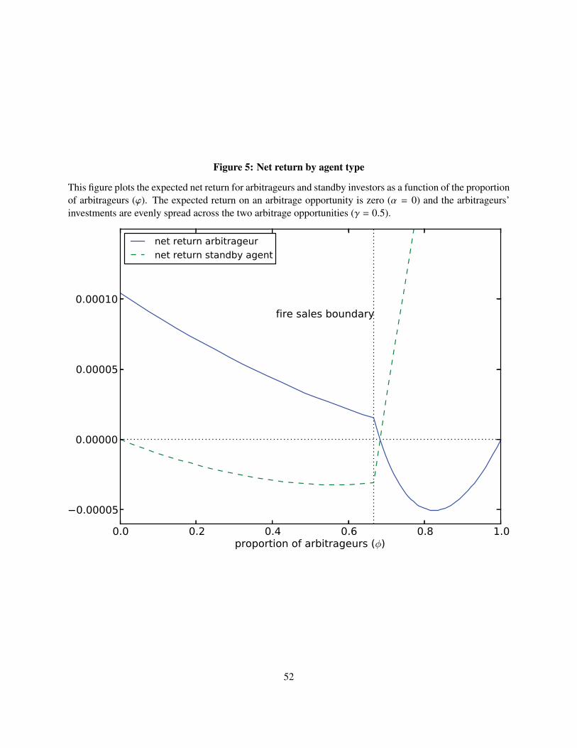
Figure 5: Net return by agent type

This figure plots the expected net return for arbitrageurs and standby investors as a function of the proportionof arbitrageurs (ϕ). The expected return on an arbitrage opportunity is zero (α = 0) and the arbitrageurs’investments are evenly spread across the two arbitrage opportunities (γ = 0.5).


0.00005

0.00000

0.00005

0.00010fire sales boundary

net return arbitrageur

net return standby agent

52

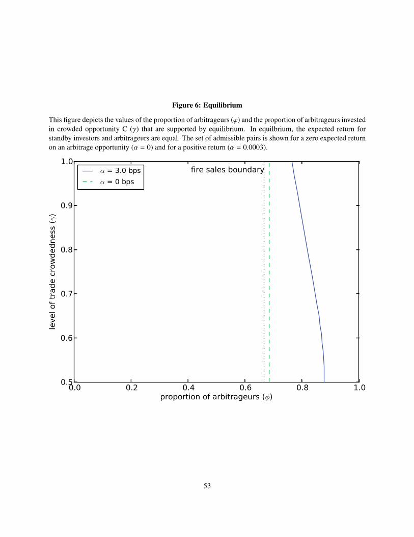
Figure 6: Equilibrium

This figure depicts the values of the proportion of arbitrageurs (ϕ) and the proportion of arbitrageurs investedin crowded opportunity C (γ) that are supported by equilibrium. In equilbrium, the expected return forstandby investors and arbitrageurs are equal. The set of admissible pairs is shown for a zero expected returnon an arbitrage opportunity (α = 0) and for a positive return (α = 0.0003).


0.5

0.6

0.7

0.8

0.9

1.0

level of

trade c

row

dedness

(γ)

fire sales boundary α = 3.0 bps

α = 0 bps

53

Figure 7: Welfare for inelastic liquidity demand

This figure depicts welfare as measured by realized private value of outside customers. These customersare the source of the arbitrage opportunities as they are liquidity demanders, i.e., they arrive in the marketearly and demand immediacy from arbitrageurs as in Grossman and Miller (1988). Their demand curve isassumed to be iso-elastic, the price is proportional to 1/q1/η where η denotes demand elasticity. η is 1/2in this figure. Panel A depicts welfare as a function of the proportion of arbitrageurs (ϕ) and the extent towhich their trades crowd (γ). Welfare at any point is measured as the distance relative to the highest possiblelevel, i.e., welfare at (ϕ, γ) = (2/3, 1/2). Panel B graphs welfare levels that can be reached in equilibrium,i.e., welfare levels for which the expected return for an arbitrageur is equal to that of a standby investor.The expected return on the arbitrage opportunity (α) is endogenous and determined by liquidity supply andliquidity demand. The graph also plots welfare levels for an exogenous α so that the effect of endogenizingα becomes visible.

Panel A: Welfare relative to highest level (ϕ, γ) = (2/3, 1/2)


0.6

0.7

0.8

0.9

level of

trade c

row

dedness

(γ)

fire sales boundary

welfare=

-55%

wel

fare

=-4

5%

welfa

re=

-35%

welfare

=-2

5%

welfare

=-1

5%

54

Panel B: Welfare levels that can be reached in equilibrium.


0.6

0.7

0.8

0.9

level of

trade c

row

dedness

(γ)

fire sales boundary

welfare=

-55%

wel

fare

=-4

5%

welfa

re=

-35%

welfare

=-2

5%

welfare

=-1

5%

α endogenous

α = 3.0 bps

55

Figure 8: Welfare for elastic liquidity demand

This figure depicts welfare as measured by realized private value from outside customers (similar to Panel Bof Figure 7 except for η = 5 instead of η = 1/2). These customers are the source of the arbitrage oppor-tunities as they are liquidity demanders, i.e., they arrive in the market early and demand immediacy fromarbitrageurs as in Grossman and Miller (1988). Their demand curve is assumed to be iso-elastic, the priceis proportional to 1/q1/η where η denotes demand elasticity where η = 5 in this figure. The figure depictswelfare level as a function of the proportion of arbitrageurs (ϕ) and the extent to which their trades crowd(γ). Welfare at any point is measured as the distance relative to the highest possible level, i.e., welfareat (ϕ, γ) = (2/3, 1/2). The graph further depicts welfare levels that can be reached in equilibrium, i.e.,welfare levels for which the expected return for an arbitrageur is equal to that of a standby investor. Theexpected return on the arbitrage opportunity (α) is endogenous and determined by liquidity supply and liq-uidity demand. The graph further plots welfare levels for an exogenous α so that the effect of endogenizingα becomes visible.


0.6

0.7

0.8

0.9

level of

trade c

row

dedness

(γ)

fire sales boundary

welfare

=-5

5%

welfare

=-4

5%

welfare

=-3

5%

welfare

=-2

5%

welfare

=-1

5% w

elfa

re=

-15%

welfa

re=

-5%

α endogenous

α = 3.0 bps

56

should fast-moving capital in crowded trades be … annual meetings...should fast-moving capital in...

Documents