ship resistance and propulsion prof. dr. p. krishna kutty...

Ship Resistance and Propulsion Prof. Dr. P. Krishna Kutty

Department of Ocean Engineering Indian Institute of Technology, Madras

Lecture - 9

Model Tests and Ship resistance Prediction Methods – II

We have been discussing about prediction of ship resistance from model test. There are

different methods for predicting the resistance from model test.

(Refer Slide Time: 00:27)

One of the method is put forward by Telfer and is known after him as Telfer's prediction

method. We can see here, the graph shows total resistance coefficient usually is put as 10

cube c t because of the value of numerical values it is quite small. Usually it is better to

plot you know 10 cube c t and against the Reynolds number here. So, here in the Telfer's

method, it tries to satisfy a Reynolds number and a Froude number from the model test.


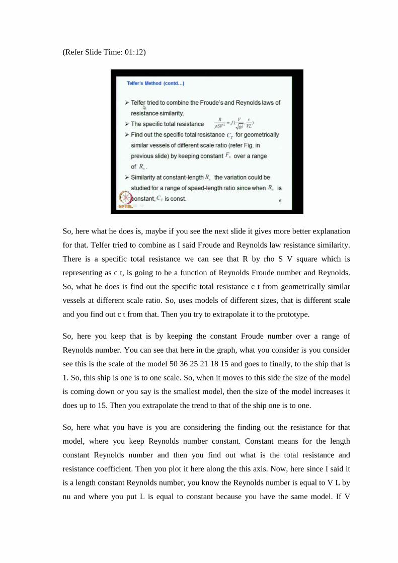
So, here what he does is, maybe if you see the next slide it gives more better explanation

for that. Telfer tried to combine as I said Froude and Reynolds law resistance similarity.

There is a specific total resistance we can see that R by rho S V square which is

representing as c t, is going to be a function of Reynolds Froude number and Reynolds.

So, what he does is find out the specific total resistance c t from geometrically similar

vessels at different scale ratio. So, uses models of different sizes, that is different scale

and you find out c t from that. Then you try to extrapolate it to the prototype.

So, here you keep that is by keeping the constant Froude number over a range of

Reynolds number. You can see that here in the graph, what you consider is you consider

see this is the scale of the model 50 36 25 21 18 15 and goes to finally, to the ship that is

1. So, this ship is one is to one scale. So, when it moves to this side the size of the model

is coming down or you say is the smallest model, then the size of the model increases it

does up to 15. Then you extrapolate the trend to that of the ship one is to one.

So, here what you have is you are considering the finding out the resistance for that

model, where you keep Reynolds number constant. Constant means for the length

constant Reynolds number and then you find out what is the total resistance and

resistance coefficient. Then you plot it here along the this axis. Now, here since I said it

is a length constant Reynolds number, you know the Reynolds number is equal to V L by

nu and where you put L is equal to constant because you have the same model. If V

changes during the small range in the velocity, that is V of the model goes by the change

as per the Froude assumption, that is the V m is equal to V s by square root of lambda.

So, that is the variation what you see here at the this axis. So, that is what is called. So,

here you get the resistance for that model at different speeds or different Froude number,

actually for different Froude number you have each point is a Froude number. So, for a

particular Froude number you have the resistance and you will just plot it here. Now, you

go to the next model which is a bigger one the scale is 36. So, for you run the same we

make the model run the model in the towing tank. Then you find out what is the at each

Froude number what is that total resistance and resistance coefficient. Similarly, you do

it for the different Froude number and you get this curve.

So, you repeat that for a bigger model scale 25. So, you have Froude number varying like

this and you get the total resistance coefficient. Then you do for the next bigger model 21

scale, you got this curve go for the bigger one you got this curve and higher one. So, you

get got a set of curves for from one curve from each model. So, which represents the

total resistance coefficient. So, now what you do is you connect the points of the same

Froude number here you can see the Froude number is 0.26 this line representing the

0.26 Froude number 0.25 0.23 0.22 like this, each line representing each number.

So, how you obtain got is we have the Froude number here that is 0.28, next curve you

get 0.28, next curve you take another point. You join all these points you get this line this

line up to 15. So, you have tested model up to a scale of 15, that is the biggest model you

have tested 15 factor is equal to 15. Now, you connect this point next Froude number of

0.25, we can see this 0.25. So, you have connected the similar Froude number points we

have taken up to this point. So, you have done the same thing for other Froude number.

So, you get these curves up to 15.

Now, what you do is you extrapolate this curve to this value the scale of one is to one

extrapolate this curve these curves to the ship that is 15 scale to the scale of one. That is

the ship. So, that is how the Telfer prediction method, Telfer uses the prediction method

where he tries to satisfy the Reynolds number and also the Froude number. Here you can

see that this line which is given by the frictional resistance line which we have already

discussed it is a Schoenherr formula frictional resistance, which we discussed in one of

the previous classes. So, this is a line representing that, it has been observed that these

constant Froude number lines are following almost parallel same trend as this line.

So, he has used this as the reference line for the extrapolation of these lines to one scale.

So, this is based on the observation, this line has been to the following or parallel to this

up to this range and we have the information for this line up to this. So, we just use this

as a lines parallel to that. So, that is how we got the resistance of the ship. So, here that is

what he tried to combine both Froude’s and Reynolds laws. We know that resistance

coefficient is given by Froude number and Reynolds number is trying to satisfy both. So,

here you find out the specific resistance rho to c t for geometrically similar vessels. It is

not one vessel he has tried many different small model vapour model bigger model and

much bigger one, of different scale ratio by keeping constant Froude number.

We have seen that is constant over a range of Reynolds number. So, we consider for the

whole range of Reynolds number, here is a Froude number of curve 4.26, here is Froude

number curve 4.25 like that. So, that is how what it explains here. Similarly, at constant

length Reynolds number, the variation could be studied for a range of speed-length ratio

since the Reynolds number is constant c f is constant. So, here that is what is done. So,

here it is assumed to be a constant length Reynolds number, l is kept constant because of

same model. So, this is studied for different Froude number here is this one for different

Reynolds number depending on that you have this. So, he is trying to satisfy both in the

same test.


Thus only change in C t and C only change in that resistance coefficient total resistance

coefficient with Froude number would be due to wave-making. So, what do you consider

is only change in C t with Froude number, if you consider along the same Reynolds

number and Froude number only change is due to wave-making. All contours of constant

Froude number are mutually parallel, that is what you have seen all the constant lines are

see all these lines are parallel that what is mentioned here, mutually parallel C t contours

of constant length Reynolds number against Froude number these are also parallel to

each other. That is these curves are also parallel these curves are also parallel to each

other.

So, that is C t contours of the constant length Reynolds number against Froude number

base are also parallel to each other. That is a vertical slanted line in the figure that is what

we have seen. Extrapolate the model values to that of the ship range that is what I said

you extrapolated that. Then you what it is that is a model resistance then you give

roughness allowance and air-resistance allowance needed to be added to ship’s C t. So,

which is not present in the model test, so the roughness allowance, there is the ship

model surface is more very smooth and ship surface is not so smooth.

So, the roughness is different and you have to give extra allowance to account for the

variation in the roughness between the model surface and ship surface. Air resistance is

not measured. So, give allowance for the air resistance also, from which you get total C t

of the ship. So, see from the C t of the model you put these two allowances you get the C

t of the ship and obtained in the extrapolation.


The C t curves for constant Froude number is nearly parallel to the Schoenherr’s formula

that is what I shown before you can see here. These curves are almost parallel to this

curve this is Schoenherr’s formula for slat plate resistance put forward by. So, you have

this formula here. So, this is isolating C f it is not C p. So, here you have that. So, this

line can therefore, be used to reference line by the parallel extrapolation. So, this line is

used the Schoenherr line is used for the parallel extrapolation because see you can if you

consider you have points only up to this point.

Now, you are extrapolating a long way to the ship. So, even a small change in the trend

makes a lot of difference when it reaches here. So, you do not want that to happen you

minimise the error and it has been found that parallel to this which gives the trend is

more reliable and hence the lines are these lines are made parallel to the Schoenherr line.

So, that is this line can therefore, be used as a reference line for the parallel

extrapolation. The ship resistance now you get you have got C t s from which

multiplying it by half rho, the ship wetted surface area velocity square that gives the total

resistance of the ship.

So, that is how the ship resistance is predicted from model test by Telfer and he tries to

satisfy the Reynolds number and the Froude number in the model test, but there are a lot

of disadvantages or problems with Telfer's method, Reynolds number distance from

model to ship is very large.


We have seen that Reynolds number which you consider from model is Reynolds

number here where as the ship is not Reynolds number here. So, this is a long variation

the gap is. So, high so extrapolation may lead to problems. So, that is very large and

hence even a minor inaccuracy on the extrapolation can lead to large error on the

forecast. So, any prediction of the ship resistance from the model test and which got

extrapolated over such a gap, can lead to inaccuracy, major problem there, for big

models kinematic dissimilarity around a ship model due to tank wall.

So, if you are using he has used the models say 50 to 15, when it comes to the scale of 15

the model size is. So, big the big models there is mainly the breadth of the model and it

may create a tank wall effect the tank is not wide enough. This may create tank wall

effect and that lead inaccurate prediction. So, hence that is what he says you see for big

models kinematic dissimilarity around a ship model due to towing tank wall interference

towing tank wall interferes and resistance recorded will be wrong.


Wall effects also leads increase in resistance, that is what I said wall effect again leads to

increase in resistance, when testing small models so the lowest model is a scale of 50 that

is a very small model. So, flow over such small models become laminar the Reynolds

number is very low and the flow become laminar, which again deviates a lot from the

actual flow around the ship. Hence the kinematical similarity is totally apart. So, hence

the measured resistance is less than the actual, when turbulent flow is to be encountered

in higher ships. So, when you consider the turbulent region and the laminar region we

know that resistance coefficient is higher frictional resistance coefficient is higher and

low Reynolds number or at laminar region and frictional resistance coefficient decreases

when it goes to the turbulent region or in the higher Reynolds region number region.

Testing with a family of model, now what you have to do is you have seen that we are

using many models. We have to have models with different scales one model with 50

scale another model with 36 scale, another model with 25 scale. So, we need so many

models of different sizes, if you want to use the Telfer's method. So, model make making

is expensive and time consuming. So, you can see that a testing with a family of models

for a range of lambda required it is expensive and it is also time-consuming.

So, these are the disadvantages problems with the method. So, considering all these

aspects disadvantages and all that and cross involvement, facility limitations many of

these aspects. The method put forward by Telfer's is generally not acceptable or

practically it is not feasible. So, it is not picked up. So, we see what are the other

methods available?


Next method is Hughes method for the prediction of ship resistance from model test. So,

based on the experiments on frictional resistance of smooth plane surface in turbulent

flow Hughes proposed. So, he has considered a plane surface in turbulent flow

experiments on the frictional resistance of smooth plane surface C f. So, what he has

done is this also again based on plane surface and he has come out with the plate

frictional resistance based on the experiments. C f is equal to approximate 0.067 divided

by log 10 R n minus to the whole square this is the expression put forward by Hughes

based on his studies.


So Hughes what do I put here is the total resistance is now constituted by the base

frictional resistance at the flat plate which we have seen, using the previous formula plus

the form resistance deeply submerged double hull model. So, double hull model is the

one which I have discussed before. So, it is a deep form resistance plus free surface

resistance, that is the wave-making resistance.

So, this is a basic frictional resistance into R that is the flat plate resistance into R, R

takes care of the form resistance plus the free surface resistance. Where r is the resistance

ratio and is a constant factor for a given hull form. So, you find out what is r and that

gives that r is equal to one plus k, k is called the form factor. We will see in the next

figure, next slide what is how this is estimated one plus k and all that.


What is that is done here, what it does is you have 10 cube C t against Reynolds number

and you use the same form formula with what the Hughes formula, you can see that this

is the Hughes formula. So, this with that you plot the base line the base line here you can

see, that is based on this expression which is depending on Reynolds number. So, you

have the Reynolds number here and you use this plot is obtained from that formula.

Now, you do the model test you find out the total resistance coefficient of the model this

is a model region.

So, for different Froude number different that is what different Froude number we get

that resistance coefficient here. So, you plot that then you join it with a curve. So, you it

goes like this basically something like this. So, this is a resistance curve. So, what you do

is, now you draw lines this base line into 1.1 you get this line into base line into 1.2 you

get another line, base line into 1.3 you get another line. So, you keep doing up to I think

up to 1.5. So, you get so many lines which is obtained by multiplying this formula into

these factors. So, you get lines which come like that.

So, now at this lower region you find that the resistance curve the model resistance curve

usually goes like this it comes like this and it goes like that. So, this is a at a very low

Froude number at very low Froude number the wave making effect is less. So, the major

effect or the whole effect is coming from viscous. So, there is no wave making at very

low Froude number. So, at very low Froude number, if you do the test for few speeds at a

very low Froude number then you get the resistance exclusively by the viscous effect.

So, if you find that this trend of the curve it is coinciding between 1.2 and 1.3

somewhere here. So, interpolate that position from which you get the form factor here.

So, that is how the form factor is obtained in the from this test. So, you can see here this

one k into C f that is what is marked. So, that depends on the this curve. So, k into c f

represents the form factor.

So, the reason physical reason given for the from factor is that I think we have already

discussed about that here the formula is based on the flat plate resistance with all this it is

given thus carried out using flat plates of different length and different width in the flat

plate the flow velocity around the flat plate is different from the flow velocity around the

ship. So, maybe that i will explain using a diagram.


Suppose, you consider a flat plate consider as a flat plate. If you look from the top the

plan view it maybe, this is a plan view it is now deeply submerged. So, you are just

towing it at different speeds. Then you measure what is the force required to tow it at

different speeds. So, this length is usually taken as the ship length or model length and

this width is equal to half the average girth mean girth. So, both sides put together gives

the total. So, this represents the wetted surface area of the ship.

Now, if you look to the from the top this is the plan. Suppose that it is moving in this

way this is moving. So, that which will be the flow is in this direction. So, here the flow

is like this, almost parallel flows we get. Now, you are representing this for a ship. So,

you consider a ship model or ship, just consider. We just consider ship of almost same

length, same length. If the flow if the ship is moving with suppose this velocity is v ship

also moves with velocity v, see that because of the curvature the flow comes here

because of the curvature the ship velocity increases.

The velocity here is going to be much more than this in free stream velocity. So, this

increase in velocity increases the resistance of the ship because you know that frictional

resistance is proportional to v power 0.825. So, this velocity is the flow velocity. So, here

in the case of the ship due to this three dimensional form the flow velocity is higher

which is not accounted here. So, this expression which has been developed maybe the

Schoenherr’s formula or Hughes formula or ITTC formula where they used a flat plate

resistance. They have not considered the increase in velocity of flow due to the form of

the ship. So, that increases the frictional resistance of the ship. So, which is accounted by

that is why it is called the form that is k is called the form factor.

So, this k form factor is basically due to the change in the flow in the velocity or increase

in the flow velocity around the ship. So, that is a physical reason for such a difference.

So, that is how now you get the form factor. So, you use the same form factor for the

ship also, this shows the extrapolated values of the resistance C t s for the ship for the

ship operates at a higher Reynolds number. You can see that total value from here to here

it is 1 plus k into C f s and C f s is coming from this expression. So, that is what is done

in the Hughes method.

So, in Hughes method what he does is he uses his the formula which I said before the

same formula this is the Hughes formula for frictional resistance. Here what we say is it

represents total resistance as a basic frictional flat plate resistance plus the form

resistance plus free surface that is the wave making resistance. Now, he clubbed these

two both are having the viscosity effect. So, we just put 1 plus k into the base resistance

flat plate resistance plus the free surface resistance.

Now, he is suggesting how to find out k or 1 plus k. So, that is what is done here from

the model test once we discussed, we have the base line and then using his formula of

base line. Then you generate curves with different multiplication factors 1.1 like. So, you

get these curves you have the model test resistance for different Froude number we have

like this something like this it comes. Curve here is not exactly matching here it will be

something like this. So, that at low Froude number, you there is no wave making and the

whole thing is due to viscous effect.

So, the viscous effect you see that the resistance is more than the base line. So, this more

the additional resistance, this part is due to the three dimensional effect which affects due

to the increase in velocity, due to the form of the ship that is why it is called the form

factor. Once you get that form factor, the same form factor is taken for the ship also, with

that you and then you are extrapolating with for the ship as we did before, as we

suggested before. Then you get this curve and this total value what you call here it is the

1 plus k into C f of the ship.


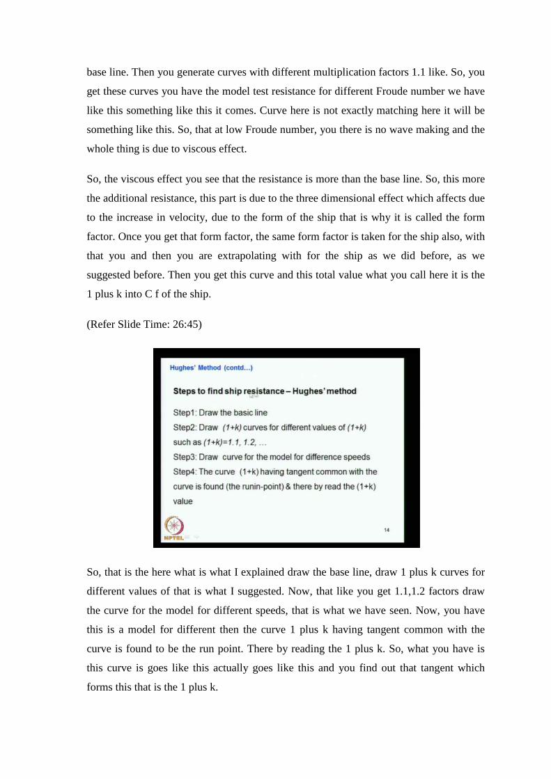
So, that is the here what is what I explained draw the base line, draw 1 plus k curves for

different values of that is what I suggested. Now, that like you get 1.1,1.2 factors draw

the curve for the model for different speeds, that is what we have seen. Now, you have

this is a model for different then the curve 1 plus k having tangent common with the

curve is found to be the run point. There by reading the 1 plus k. So, what you have is

this curve is goes like this actually goes like this and you find out that tangent which

forms this that is the 1 plus k.


So, from which you read the 1 plus k. Extrapolate it C f into 1 plus k to the ship region

that is what you have done read C w of the model at different F n subtracting by

subtracting this from the C t. So, what you do is you here you have C f plus k C f and

from there you find out what is the difference. That gives the C w. So, C w we know that

is same as C w f of model same as C w of ship. So, these two values are same only

difference here this C f value changes. So, you put C f using this formula C f s then you

put the C w here, C w is constant. Put the C w here then you get these points then you get

this curve.

So, that is based on the so read a C w model at different Froude number by subtracting C

f into 1 plus k from C t. Based on the Froude law plot C w over C f into 1 plus k to get

the C t of ship. That is this I explained, add model from to this you add that model ship

correlation allowance. That is I said due to the change in roughness due to the ship

surface change, roughness of the ship and model are different model is very smooth

whereas, for the ship it is not so smooth. The smoothness there are different reasons that

also we discussed before due to painting, due to welding joints or due to deformations of

the plate. There are many reasons for increase in roughness for the ship and which is not

present in the case of the model. So, that increase in roughness need to be accounted

when you estimate the total resistance of the ship compared to that of the model.

So, that C a there is a correlation allowance, is added to that model value. Then you get

C t s and then you find out total resistance of the ship is equal to this C t s value into half

rho S s V s square that the ship parameters better surface and velocity and density. So

you get total resistance of the ship from this that is the Hughes prediction method.


So, here that is the method which has been proposed by Hughes to estimate the form

factor. Now, we see another method called Prohaska’s method how to determine the

form factor from the model test. So, here this is the method proposed by Prohaska in

1966. So, what he has done is the 1 plus k factor the form factor vary with respect he has

given shown a curve this is for each curve for a particular l by delta power one third you

can see that. So, delta power one for the same length if you consider, delta is small, delta

power one third isn’t it.

This value will be if your delta is large that is fuller form then this value will be smaller.

So, here it is 4 5 6 7 8 that is the value. So, this side of the curve that is when it is 4

means it is the fuller form ship. That is for the same length it has a more displacement

the denominator is high, that is why the value is less. So, this region maybe referring to a

tanker ship or maybe a bulk idea and all that, so these types of vessels will have higher

form value. So, you can see the 1 plus k and against C b. So, you can see the C b value C

b is high full form and here we can see what is the form factor?

If you consider this curve the form factor is high, but when it comes to a smaller one this

l by delta power one third is small that means one power is high value 8. So, here that

means the denominator is small that is like container ship, whether the denominator is for

the same length. The displacement is less it comes in this line you can see that form

factor is less is 1 point less than 1 point 1, where here this range becomes more than 1.2.

So, that shows the indication how the body is more full the higher will be the value of

form factor is the body is fine because it is getting closer to that flat plate. The form

factor is less, if it deviates more from the flat plate concept or assumption then the form

factor effect will be more.


Prohaska proposes a method for determining the 3 d form factor, that is what is that. He

just put you put the k as the factor C v minus C f o by C f o. This is the factor he used

what is all this file is C v is the total viscous resistance coefficient of the 3 d form. So,

the 3 d form you consider you find out that the total viscous effect. Viscous resistance

that is the C v C f o is the frictional resistance of the 2 d flow that is the plate flow. So, C

f o is coming from the formula and C v is actually the measured one, due to the 3 d form.

So, that difference divided by C f o is given as k. So, where no separation you do not

consider separation here only is the here you consider only the form effect. C t is equal to

C w that is wave making resistance coefficient plus 1 plus k into C f o that is wave

making plus viscous effect. Viscous effect is C f o plus this k into C f o k into C f o is the

difference of that means actually C w plus C v you can see that k is equal to C v minus C

f o divided by C f o. So, that is this gives that C v is equal to k into C f o plus C f o that is

what is written here. So, this is same as C v which is coming from here.

So, here C w is the wave making resistance coefficient. We already know that C w is the

function of that is R w, you know already R w is proportional to V power 6 you have

derived you know the previous classes. So, C w is equal to R w by half rho S V square.


So, that means C w is proportional to C w is proportional to now V power 4 or we know

that Froude number is equal to V by root g L. So, we can say that this is now

proportional to Froude number is to 4. So, C w is proportional to Froude number raised

to 4. So, that is how we have written like that C w is y, y is a constant into Froude

number raised to C w is proportional to Froude number raised to 4. So, y is a coefficient

and F n is the Froude number.


So, in the same thing it is what I have explained R w is proportional to V power 6 and C

w is given by this relation and from which finally, you get this proportional distribution.

So, what you have is, if you look to the above relation here C t C w and all that C w is

now is equal to y into F n raised to 4.


So, from here you write here C t is equal to C w into we have C t is equal to C w plus

one plus k into C f o. We know C w is coming from here. So, that is equal to y into F n

raised to 4 plus 1 plus k into C f o or we can write C t by C f o is equal to 1 plus k plus y

into y or y F n raised to 4 by C f o. So, that is what we write. So, here that is what is

shown you can see that C t by C f o is equal to 1 plus k. So, I think that is correct plus y

this is y F n raised to 4 by C f o. So, that is how you write that expression.


So, what does that mean this is if you write this is something like a equation of a straight

line y is equal to m x plus c this is y c is this is referring to m x that is if you write a if

you plot a straight line with this as y and F n raised to 4 by C f o as x, then you get a

straight line, so equation of a straight line. So, that is what is done you plot C t by C f o

divided by against F n raised to 4 by C f. You get a straight line the slope of this straight

line is y and intersection is equal to 1 plus k. You can see that C t by C f o is equal to 1

plus k.

So, here this is the vertical axis same as y and this is the x axis which is x. So, you see

this y is equal to m x plus c. So, C is the intersection which is 1 plus k. So, you have this

red dots the values coming from experiments at low Reynolds number and low Froude

number. These plots for using this what you do is you find out what is C t, C t is obtained

the total resistance from which you get C t. Now, you find out C f o from I T T C

formula or any of the formula, that is also known to you for that low Froude number.

So, you can find out this quantity and similarly, you know what is the Froude number

and then the Froude number raised to 4 this also you can estimate from that model

parameter. So, these two quantities are known. So, you plot this and this. Now, you get

the experimental points the red dots here, you connect of it a straight line to these points

then this straight line intersects this axis and that is equal to 1 plus k. So, you get this

value here. So, here this intersection that is how you get the intercept form factor. This is

the method suggested by Prohaska.

So, you run the model at low Froude number and you get the resistance value. Then you

find out what is the C t of the model you find out what is the C f o from the I T T C

formula similar formula. So, you find out this ratio here. Now, you find out the model is

done run at different Froude number. So, if you know that, what is the Froude number

divided by the corresponding C f o again from I T T C, this ratio also is obtained from

the model test. Now, you plot this ratio against this ratio.

So, you get few points like this. You know this experiment you do not get just very

smooth simple line. So, you just fit a straight line to that because you know that is almost

following a straight line pattern linear variation, this when you put it here or extrapolate

to this it intersects the axis and this intersection which is supposed by 1. So, this value

directly gives 1. So, that is what is written here. So, here the model should be run at very

low speed generally Froude number between 0.1 and 0.22. So, that is what is done in the

Prohaska’s method. That is how the models how you find out the form factor from the

model test. The same form factor holds good for the ship also.


So, the uncertainty of measuring the resistance at very low speed is a relatively large. So,

when you measure the resistance is very low at very small Froude number, very low

speed. So, measurement become also becomes difficult when you use a small quantity.

This means that it is difficult to determine the run in point that is you have seen the

Hughes method what is the run-in point that is the slope which comes during the bottom.


So, the run-in point is if you consider the total resistance if you if you put a C t against

Froude number, we get a value a curve something like this. So, here and you have the C f

value, C f coming maybe like this because you know, this is C f and we know it is

proportional to V power minus 0.175. So, it goes like this and the total resistance curve it

just initially like this because this region only is the frictional resistance. Then it goes

like this, wave making fix up in this region.

So, this is called the run-in point. So, this is going to be right. So, this is accounting for

the form factor k. So, that is the point what it is called the run-in point. So, that is here

what you see it is the run-in point, is that is the slope that reach. For fuller form that is

like I mean bulk idea or the plot is concave curve, you can see that it is not it is different

1 plus k and are speed dependent. We see that what happens to the, I power you can see

that it is not a straight line if it is a full form ship.


You can see that this is not a straight line the points you see here it is coming like a

concave curve. So, it is curving like that because for fuller form ships, the resistance we

have seen is generally V power 6, but for fuller form ships the resistance is not V power

6. it maybe V power 7 or V power 8. So, when you use this relation it is not going to be a

straight line representation. So, what you have to do is you may have to change increase

the F n raised to 4 to F n raised to 5 or F n raised to 6.

Then you get a straight line otherwise you get such a curve like this. So, what is that for

fuller form the plot is concave curve that is what you see 1 plus k and y are speed

dependent it may be better to use the power for F n between 4 and 6. So, F n we have

used previously power 4. So, here it suggests that you use something more than 4 maybe

5 or even 6.


So, that is how that is a Prohaska’s resistance prediction method or Prohaska’s method of

predicting form factor not resistance actually the form factor. Then we have seen now the

resistance prediction method using Telfer's and also we have seen that it is practically not

acceptable. Then we have seen the Hughes method where he has considered the form

factor also into effect. Next we considered the Prohaska’s method to determine the form

factor. So, these are the things what we have done.

Now, we have two prediction methods put forward by I T T C, initially put forward in

1957 prediction method and later it was replaced by I T T C 1978 method. So, the

difference between 57 and 78 methods are, in 78 method, the form factor is also

accounted for whereas, in 57 method the form factor is not considered. So, with this we

will conclude the today’s class and resume next day.

Thank you.

ship resistance and propulsion prof. dr. p. krishna kutty...

Documents