Dis cus si on Paper No. 18-006

Sharing is not Caring: Backward Integration of Consumers

Christian Spindler, Oliver Woll, and Dominik Schober

Dis cus si on Paper No. 18-006

Sharing is not Caring: Backward Integration of Consumers

Christian Spindler, Oliver Woll, and Dominik Schober

Download this ZEW Discussion Paper from our ftp server:

http://ftp.zew.de/pub/zew-docs/dp/dp18006.pdf

Die Dis cus si on Pape rs die nen einer mög lichst schnel len Ver brei tung von neue ren For schungs arbei ten des ZEW. Die Bei trä ge lie gen in allei ni ger Ver ant wor tung

der Auto ren und stel len nicht not wen di ger wei se die Mei nung des ZEW dar.

Dis cus si on Papers are inten ded to make results of ZEW research prompt ly avai la ble to other eco no mists in order to encou ra ge dis cus si on and sug gesti ons for revi si ons. The aut hors are sole ly

respon si ble for the con tents which do not neces sa ri ly repre sent the opi ni on of the ZEW.

Sharing is not Caring: Backward Integration of

Consumers

Christian Spindlera, Oliver Woll

b, Dominik Schober

c

January 19, 2018

Abstract

A new type of player occurs in the sharing economy: a vertically integrated consumer who

owns production facilities and has direct market access, often termed “active prosumer”. The

prosumer faces a trade-off between market transaction cost and substantial strategic potential

to influence both market demand and supply by her decisions. We discuss optimal marketing

and production decisions in light of this trade-off. An empirical application to the German-

Austrian electricity market demonstrates substantial incentives for active market participation

by recently added decentralized renewables production. Prosumers can achieve considerable

profit increases by switching roles of net market supplier or customer.

Keywords: Active Prosumer, Capacity Withholding, Self-Supply, Vertical Integration, Con-

sumer Production, Market Participation Cost

We acknowledge helpful comments by Władysław Mielczarski, Yossi Spiegel, and Franz Wirl,

and are grateful for discussions at the 15th IAEE European Conference (Vienna, Austria)

and 23rd YEEES Workshop (Lodz, Poland). The usual disclaimer applies.

aCorresponding Author, University of Vienna, Faculty of Business, Economics and Statistics, Oskar Mor-

genstern Platz 1, 1090 Vienna, Austria. Email: christian.spindler@univie.ac.at

bZEW, Centre for European Economic Research, L 7/1, 68161 Mannheim, Germany.

Email: oliver.woll@zew.de

cZEW, Centre for European Economic Research, L 7/1, 68161 Mannheim, Germany.

Email: dominik.schober@zew.de

1

I Introduction

Technological developments allow for new levels of information aggregation and thereby be-

fore unthought-of market participation. On the one hand, using decentralized information

(or knowledge) is known to be one of the major drivers of efficiency as discussed already in

Hayek (1945). Lowering entry cost will typically lead to new market participants of compa-

rably small scale as is the case for the sharing economy. Offering own living space or the

own car is a massive business case due to low-transaction cost platforms such as AirBnB

or Uber. Textbook economics will then tell a story of polypolistic competition leading to

efficiency gains. On the other hand, however, an interesting and largely ignored aspect of

this phenomenon is that these “prosumers” are typically vertically integrated, combining both

production and consumption (Toffler 1980). Usually vertical integration refers to firms sell-

ing to consumers, whereas prosumers are of particular interest because the demand side is

directly involved in the integration process and strategically participates on the market.

Hence, we address the following questions: How will a marginal, vertically integrated market

participant facing residual supply and residual demand consume and produce? What are the

incentives of these new participants when they are small and – exceeding the case of the pure

sharing economy – when they become bigger? How do these incentives change when market

conditions vary?

In this paper, first, a theoretical model sheds light on supply and demand incentives for

differently sized prosumers. This new type of player in the market changes her strategic

role and decides about her degree of market participation in contrast to self-supply. The

prosumer can withhold supply as well as demand thereby increasing her lever for strategic

behavior or, in other words, for the exercise of market power. Her optimal decision is shown

to depend on current market conditions such as the price elasticity of the prosumer market

supply and demand as well as own and market marginal cost. Second, an empirical applica-

tion to the electricity sector in Germany serves to investigate the incentives of the vertically

bundled prosumer. We deem this sector to be particularly interesting, because two recent

2

developments led to a new type of “gentailer”: First, the decentralization of power generation

increases, fueled by decreasing investment costs for e.g. photovoltaic systems or wind turbines

rendering small scale generation viable (IEA Wind 2015, IRENA 2016, Comello & Reichel-

stein 2016). Second, the ownership structure changes from a traditional system of few big

generation firms towards fragmented generation being owned and operated by small agents,

such as homeowners or farmers. These own about 80% of German photovoltaics capacity

being connected to the low voltage network (see Hanna et al. 2017, Kairies et al. 2016).1

Initially, generous feed-in-tariffs led to passive supply to the market. Gradually declining

they fell below the average retail electricity price in Germany for the first time in January

2012 (BMJ 2017). This might mark the change to the active prosumer. This path may be

guided in the future by increasing automation of the smart home, but already started by

“aggregators”, companies aggregating demand or supply, such as Statkraft. We demonstrate

how these differently sized market participants are able to strategically influence the market

price and increase own profits. Moreover, this application is particularly interesting be-

cause of the many dynamic switches of the strategic role of the prosumer, oscillating between

residual monopsonist and residual monopolist (i.e. demand-only and supply-only situations).

Today it is still the most common way for a prosumer to participate in the electricity market

passively serving own demand first and selling solely excess capacity to a load-serving entity

(LSE) or distribution system operator (DSO) at a predetermined, fixed price.2 Thereby the

prosumer is deprived of any adaption to dynamically changing market conditions. Hence,

we term this agent “passive prosumer”. In contrast, the “active prosumer” currently gains

importance as a recent report by EPEXSpot, a European electricity traders’ association,

underlines (Töpfer et al. 2017). In contrast to small consumers such as households still wait-

ing for the technological preconditions enabling them to play an active role in the market,

so-called “aggregators” already participate in the game today. These companies directly offer

production on the markets aggregating multiple production units and, furthermore, they be-

have strategically adapting their bidding behavior to (negative) market prices as an analysis

of aggregated day-ahead bidding functions shows. The European Commission acknowledges

3

their importance by including the following definition into their ‘Winter Package on common

rules for the European electricity market’: aggregators are “market participant[s] that com-

bine [. . . ] multiple customer loads or generated electricity for sale, for purchase or auction

in any organised energy market.” (EC 2007)3,4 This development is similar to other markets,

where service providers take over the role of aggregators. These parallels can be found with

Uber aggregating supply to find differentiated, time-dependent prices for a request, or tour

operators starting to offer mini-bus rides. Similarly, services handle keys through AirBnB

and allow for price information exchange influencing pricing of flats. However, in other mar-

kets prosumers are already comparably big: Amazon and Google e.g. can use their servers

for own calculations and services or sell the computing power on according spot markets.

The application to the German-Austrian electricity market demonstrates the empirical rele-

vance of these theoretical considerations. Estimating market demand and supply functions

from bid data we simulate how varying production capacity impacts the prosumer’s incentive

to optimally bid into the market and produce for own consumption. This market power effect

is shown to increase whenever capacity increases similar to many models analyzing abusive

market power. This case is particularly interesting, because even for very small prosumers or

aggregators and in less tight equilibria, it is shown to be optimal for the prosumer to influ-

ence the market equilibrium. We investigate varying scarcity situations throughout the 8760

hours of the year5. This differs from typical models of market power where market power

issues mainly arise in peak hours whereas there are no or little markups in off-peak hours

(see e.g. Joskow & Tirole (2007), Borenstein et al. (2002), Wolak (2003)). The prosumer

may raise her profit per production unit from 0.5 to 10.2 EUR/MWh even in the range of

moderate market shares from marginal size up to 10 % of maximum demand.

In the general setup of our model, however, we abstract from the electricity market and focus

on the strategy to decide for each period about the quantity offered and demanded on the

market. The insights are then also useful for other markets where the decision between self-

supply and offering a good on the market matters. Depending on the prosumers’ marginal

4

cost and the relation of the prosumer’s production capacity (or actual production) to his

demand, we find it to be optimal for the prosumer to strategically offer or withhold demand

and supply capacity around the market equilibrium. Thereby she can shift the industry’s

aggregate demand and supply functions in two directions: the prosumer can try to increase

the market clearing price e.g. by adding her demand to the market and thus benefit from this

higher price with all of his production or by withholding part of his production capacity; or

she can try to decrease the market clearing price e.g. by offering as much generation capacity

as possible. Important requirements are the possibility to actually participate and bid in a

market, e.g. via a trading license; and an independent market maker who aggregates demand

and supply bids to determine a unique market clearing price. In the electricity market, these

requirements are fulfilled e.g. at the day-ahead market at EPEXSpot.

We investigate optimal sales and sourcing as well as production decisions of a vertically in-

tegrated customer who owns production facilities6. She faces both an elastic market demand

and supply. Moreover she faces a fixed per-unit cost of trading on the market, in particular

transaction cost (e.g. trading cost, act of renting out apartment), transport cost (e.g. elec-

tricity network usage) and own opportunity cost (e.g. reduction of consumption (renouncing

on living space)). Thereby, the prosumer has a strategic potential to influence the market

price, but it depends on her entry cost7. This is in the spirit of a Cournot game, in which the

player can also change the market price altering total market quantity. In contrast, in this

paper market opponents do not react. The focus is on the prosumer’s incentives to influence

the market price, whereas the reactions of other players are, first, second order effects and,

second, straightforward and known from the literature. Third, this exogenous treatment of

the market equilibrium has the very pragmatic advantage that it offers the possibility to ig-

nore market power issues in the rest of the market. In peak load systems, such as electricity,

market power varies on an hourly basis. Modeling prosumer behavior as a decision problem

thus is an elegant and realistic way of investigating her optimal production and trading de-

cisions. It is discussed theoretically how the prosumer makes optimal sales and sourcing as

well as production decisions and thereby influences supply and demand to increase her profits.

5

Two facts are worth mentioning with regard to characteristics of trading markets. First, it

is completely rational to be supplier and customer at the same time. This is a well-known

result in the finance literature derived from the market participants’ need to hedge market

risks. In the PJM electricity market, Longstaff & Wang (2004) find all wholesale market

participants to take an active role as supplier, customer or both at any point in time (see p.

5). They also find empirical evidence for results shown by (Bessembinder & Lemmon 2002)

indicating that producers and retailers have an incentive to hedge forward, in turn appearing

as both short term market customers and suppliers. Intermediate wholesale market risk can

be either hedged or avoided by vertical integration, which makes the latter rational whenever

the first is not perfectly consumable. However, production cost as well as retail demand risk

prevail making simultaneous supply and demand side bids rational. It is therefore not sur-

prising to find our prosumer to switch between the different roles as a (residual) monopolist

and monopsonist and many hybrid cases in between8. Second, vertical integration may be

advantageous9. Raising rival’s cost is a classical example (see e.g. Ordover et al. (1990),

Salinger (1988), Riordan (1998), Hastings & Gilbert (2005), Riordan (2008), Spiegel (2013)).

Without further structural adjustments of competitors (vertical integration on their part),

the integrated firm can increase sales and profits or even drive the worse firm out of the

market. In addition to arguments already discussed in this stream of literature, we consider

costs of market participation, which represents only an option for a consumer, and the op-

tion of altering market demand. In particular for smaller prosumers we find it unprofitable

to influence the market equilibrium. However, this changes considerably already for small

market shares, which can easily be achieved by aggregators such as Vattenfall on the German

market (see Töpfer et al. 2017).

The closest analytical description of prosumers in particular can be found in literature on

vertical integration, in particular with Bushnell et al. (2008) and Mansur (2007). Both con-

tributions are based on so-called “gentailers”, i.e. electricity generating companies integrated

to the retail market, who still have to forecast their final customers’ demand. The authors in-

6

corporate the internal procurement of electricity as long(er) term bilateral contracts, with the

gentailer ultimately showing up either as net-seller or net-buyer on the (day-ahead) market.

However, since they argue that retail prices are usually highly regulated and hence predeter-

mined, as well as that demand is perfectly inelastic, any strategic component of self-supply

vs. market participation is missing. This also holds for Boom (2009) who introduces retail

competition by enabling consumers to switch to the retailer with the lower price. In contrast

to e.g. avoiding double marginalization, we argue that organizational theories explaining

vertical integration e.g. via transaction costs or enhanced decision rights do not apply for

small scale prosumers. This is because contracts with a local load-serving entity which also

includes supply security compares to the risk of investing in own generation along with the

financial burden and the complex possibilities of selling the production in the different elec-

tricity markets (see Bresnahan & Levin 2012, Joskow 2010).

Prosumers as new market participants also receive particular attention in electricity mar-

ket literature. This includes a special issue in the IAEE Journal “Economics of Energy &

Environmental Policy” (2017, Vol 6/1) on ProSumAge, i.e. prosumers who also have the

possibility to store their generation (see Green & Staffell 2017). In general, the contributions

focus either on the use of flexibility or storage for optimal bidding strategies e.g. during

the day (e.g. Shirazi & Jadid 2017, Ottesen et al. 2016); or on system models extended

by allowing for prosumers to participate: the result of the prosumer’s profit maximization

serves as input for a cost minimization problem of an independent system operator who is

supposed to find the least expensive way to meet demand when also taking transmission line

constraints, loop flows etc. into account (e.g. Rigo-Mariani et al. 2014, Schill et al. 2017).

These applied simulations, however, usually consider the market clearing price as exogenous

to the prosumers’ decisions.

To summarize, we claim that there is a new kind of agent, the active prosumer, who has a new

possibility to participate in the market. To address the issue of implications for the market

and whether active participation actually is profitable, we set up a theoretical model in section

7

II to analytically derive the optimal decisions for a single prosumer facing a competitive fringe,

relaxing the price taking assumption. We show conditions for when and how to adjust market

participation to yield a profit gain compared to passive presumption, which depends on the

marginal costs of the prosumers’ production unit, demand and supply elasticities as well as

on the relation of prosumer’s own demand and production capacity. Section III contains

an empirical calibration of the model, based amongst others on hourly demand elasticities

estimated using bidding data from the German-Austrian day-ahead electricity market. We

illustrate the bandwidth of different prosumer sizes ranging from the small household up

to classical production and retail supply companies, who might take over the role as an

“aggregator”. Depending on the technology used and the according prosumer’s production

costs we find many strategic role switches and altering bidding behavior. We discuss the

results and conclude in section V.

II The Model

Nomenclature

qPSd demand purchased on the market ps, pd inverse supply and demand functions

qPSs production offered on market as, ad intercepts of supply and demand functions

cPS production costs of prosumer’s production unit QPSs production capacity of prosumer

cmarket maximum costs of generating units available QPSd capacity needed to satisfy own demand

⌘d slope of demand function Qmarketd maximum market demand (excl. prosumer)

⌘s slope of supply function Qmarkets production capacity of competitive fringe

II(i). Model Setup

Our modelling framework comprises a residual prosumer optimizing profit in a market with

given demand and supply. The prosumer’s profit is ⇡PS (see Equation (1)), where p˚ “fpqPS

s , qPSd q denotes the market clearing or equilibrium price and ⌧ the additional costs for

purchasing on the retail market, like e.g. transaction or transmission costs. The three terms

capture, first, the revenues from selling production, second, the costs for covering (remaining)

8

demand on the retail market, and third, the prosumer’s costs for using the production unit.

Note that the objective function does not contain any utility the prosumer may gain from

using the amount demanded in each period. We assume that the demand in one period is

fixed and the only consideration that remains for the prosumer is how to cover this demand

at minimum costs.

⇡PSpqPS

s ,qPSd q “ p˚pqPS

s q ´ pp˚ ` ⌧qpqPSd q ´ cPSpqPS

s ` QPSd ´ qPS

d q(1)

The prosumer has the following two decision variables: First, qPSs denotes how much produc-

tion capacity QPSs is offered on the market; and second, qPS

d denotes the amount the prosumer

purchases on the market. We impose the restriction that the prosumer’s demand QPSd must

be fulfilled at every instant and that shifting or withholding demand is not possible. Hence,

own production capacity must be used for residual demand qPSown “ QPS

d ´ qPSd , i.e. for self-

supply. However, qPSown and qPS

s do not have to add up to total production capacity, i.e. the

prosumer can withhold capacity from the market e.g. by choosing to use this capacity on

a different, e.g. subsequent, market or by withholding it completely. We assume that the

prosumer does not incorporate possible profits on other markets into his optimization. Since

our model is deterministic and the prosumer has perfect foresight of (his influence on) the

market clearing price, assumptions regarding the prosumer’s risk attitudes are not necessary.

This unique market clearing price p˚ is determined for each hour by an independent authority

that collects and aggregates demand and supply bids – i.e. price-quantity combinations – and

intersects the resulting step functions. We deviate from the fact that these aggregated supply

and demand functions are step functions by approximating them linearly. Most importantly,

we allow the prosumer to actively participate on both sides of the market by deciding whether

to enter the market and to thereby introduce a step or not. Figure 1 depicts the effect of

adding a step to the supply function – the same logic also applies to the demand side of the

market. The new, dashed step function is again approximated by a linear function (dashed).

The demand and supply functions, pd and ps, respectively, are stated in Equations (2) and

(3). It is important to note that in this linear setup the maximum willingness to pay of

9

(a) (b)

Figure 1: Schematic PS Effects on the Supply Function: (a) PS Enters, and (b) PS Exits the

Market

demand ad, the minimum ask price of supply as, and the maximum production costs cmarket

do not change when a prosumer enters or exits the market. This results in a rotation of the

functions, i.e. a slope change and constant intercepts.10 The parameters ⌘d “ adQmarket

dand

⌘s “ pcmarket´asqQmarket

sdenote the slopes of the demand and supply function as ratios of vertical and

horizontal intercepts/cutoff points; ↵ “ qPSd

Qmarketd

and � “ qPSs

Qmarkets

incorporate the respective

market size of the prosumer and depict the impact of the prosumer’s decision variables on

the slopes. If the prosumer decides to not participate in the market, ↵ “ � “ 0 and the

slopes remain unchanged; if he participates, dpd

d↵ ° 0 and dps

d� † 0 holds; and Q “ rqPS, q´PSsdenotes the amounts produced and demanded at the time of delivery, i.e. the quantities all

the market participants committed themselves to.

pdpQ,↵pqPSd qq “ ad ´ ⌘dp1 ` ↵q´1 ¨ Q(2)

pspQ,�pqPSs qq “ as ` ⌘sp1 ` �q´1 ¨ Q(3)

We also assume that the prosumer demands at every possible price based on the idea that

in the short term demand cannot be shifted, i.e. the prosumer’s individual demand function

is completely inelastic. In addition, the prosumer also cannot shift his supply e.g. by storing

production. This does, however, not affect our results, because the prosumer does take pro-

duction costs cPS into account for deriving the optimal bids (see Section II(iii).) and does not

produce, if p˚ † cPS. Modeling demand and supply as nonlinear functions would potentially

10

allow us to better depict e.g. increasing marginal costs of additional supply based on different

production technologies. However, whereas the effects to be shown remain the same this un-

necessarily complicates the optimization, and the empirical calibration in Section III allows

us to depict different effects of the prosumer’s supply and demand decisions on the market

clearing price as it is based on different elasticities and hence on different slopes for each hour.

The prosumer’s decisions affect both functions simultaneously which leads to a multiplicity

of realizable market clearing prices depicted by the shaded area ABCD in Figure 2. Point A

with the according market clearing price pA and quantity qA results whenever the prosumer

decides to not participate in the market at all, i.e. by either producing exactly the amount

needed for self-supply or by reducing overall demand to 0 (not possible in our setup). In B

the prosumer satisfies all of his demand with his own production and offers excess production

on the market. Combination C is attained with full market participation of the prosumer on

both the demand and the supply side, and D depicts the situation of a pure consumer, i.e.

without making use of any production capacity. Any equilibrium in the lighter shaded area

BEC cannot be reached, because whenever the prosumer reduces his market demand qPSd he

has to use part of his own production capacity thereby also limiting or reducing the possible

impact on the supply function.

A few crucial assumptions also need to be addressed: First, we depict the market environment

as a uniform-price double-sided call auction with Cournot competition. Relaxing the price-

taking assumption, the prosumer decides about the quantities to place in the auction, being

faced with a price-taking competitive fringe. Furthermore, we assume that the production

capacity has already been built which leaves only the decision about how to optimally use it

in the market. In addition, the installed production capacity in the market, Qmarkets ` QPS

s ,

is always high enough to provide even the highest possible demand (including the prosumer),

i.e. shortages cannot occur and importing is not necessary. Lastly, we focus on repeating

short term decisions – e.g. on a market where these auctions are held hourly leading to

hourly market clearing prices – and we exclude the possibility to store production or to shift

demand in time to benefit from or to avoid high prices, respectively. Even though this paper

11

Figure 2: Window of Attainable Market Clearing Prices and Quantities

and the model are motivated by the German-Austrian hourly day-ahead auctions held by

EPEXSpot as well as by characteristics of the electricity markets, the general model applies

to any situations where the assumptions above are met.

II(ii). Optimal Prosumer Behavior

In their most general form, the effects of the decision variables can be disentangled into

direct and indirect effects, captured in Equations (4) and (5) by the first and second terms,

respectively. For completeness, we also display the intermediate effects of qPSd and qPS

s on ↵

and � where we can see that the indirect effects have different signs because Bp˚B↵

B↵BqPS

d° 0 and

Bp˚B�

B�BqPS

s† 0. Note that these fractions implicitly contain the demand and supply elasticity,

respectively.

d⇡

dqPSd

“ B⇡BqPS

d

` B⇡Bp˚

Bp˚

B↵B↵

BqPSd

(4)

d⇡

dqPSs

“ B⇡BqPS

s

` B⇡Bp˚

Bp˚

B�B�

BqPSs

(5)

Partially solving (4) and (5) allows us to derive conditions for each of them to occur. In (6)

and (7) the generally formulated left hand sides state that, for example, if the total effect

12

of additional market demand on the profit is positive, i.e. if d⇡dqPS

d° 0, then the prosumer

should demand as much as he can: QPSd . This is then spelled out on the right hand sides

of the same lines. Regarding the optimal amount to demand on the market, we see in the

first line in (6) that if the market clearing price including transaction fees and also including

the positive effect of market demand on the price is still strictly smaller than the prosumer’s

production costs, the prosumer should demand as much as possible. In other words, using

own production capacity for self-supply is more expensive than purchasing on the market.

The third line, on the other hand, says that if the prosumer’s market demand raises the

market clearing price including transaction fees to a level above his production costs cPS – or

if the price is too high even without the prosumer’s demand – the prosumer will use all of his

production capacity for self-supply. Should this capacity be sufficient to cover the prosumer’s

demand, i.e. QPSs • QPS

d , market demand will be 0; otherwise the remaining demand must

still be purchased on the market. The same logic applies for the optimal amount to sell on

the market stated in (7). The additional constraint that part of production capacity may be

bound by using it for self-supply is captured by QPSs ´ QPS

d ` q˚,PSd . This formulation also

means that the prosumer favors self-supply over purchasing on the market due to transaction

costs. The letters X and Y stand for the isolated decision variable derived from setting the

respective total derivatives d⇡dqPS

dand d⇡

dqPSs

to 0 (see Appendix A).

q˚,PSd “

$’’’’’’’&

’’’’’’’%

max ifd⇡

dqPSd

° 0 ñ QPSd if p˚ ` ⌧ ` B⇡

Bp˚Bp˚

B↵B↵

BqPSd

† cPS

Y ifd⇡

dqPSd

“ 0 ñ Y if p˚ ` ⌧ ` B⇡Bp˚

Bp˚

B↵B↵

BqPSd

“ cPS

min ifd⇡

dqPSd

† 0 ñ maxp0, QPSd ´ QPS

s q if p˚ ` ⌧ ` B⇡Bp˚

Bp˚

B↵B↵

BqPSd

° cPS

(6)

q˚,PSs “

$’’’’’’’&

’’’’’’’%

max ifd⇡

dqPSs

° 0 ñ QPSs ´ QPS

d ` q˚,PSd if p˚ ` B⇡

Bp˚Bp˚

B�B�

BqPSs

° cPS

X ifd⇡

dqPSs

“ 0 ñ X if p˚ ` B⇡Bp˚

Bp˚

B�B�

BqPSs

“ cPS

min ifd⇡

dqPSs

† 0 ñ 0 if p˚ ` B⇡Bp˚

Bp˚

B�B�

BqPSs

† cPS

(7)

13

The optimal decisions for q˚,PSd and q˚,PS

s can be described using a case distinction (see (6)

and (7)) that is based on the signs of the total derivatives of (4) and (5). Conveniently,

this allows us to uniquely describe 9 different attainable market equilibria which we already

graphically described in Figure 2 above and which we summarize in Table I. Again, there

are the 4 “corner cases” A-D, the lines connecting and confining the feasible set, e.g. BC, as

well as the “interior” solution ABCD describing the area between.

Table I

Comparison of Optimal Decisions: 9 Cases

d⇡dqPS

d† 0 “ 0 ° 0

° 0 B BC Cd⇡

dqPSs

“ 0 AB ABCD CD

† 0 A AD D

We further proceed by combining the results of (6) and (7) according to Table I. We know,

for example, that in Case A the prosumer uses all of his production capacity for self-supply

and does not offer any excess production on the market (assuming that his production capac-

ity is larger than his demand). This translates to qPSd “ 0 and qPS

s “ 0. Plugging this into

the partially solved total derivatives, the first equation or inequality in each case is derived

from d⇡dqPS

d; the second is derived from d⇡

dqPSs

. As we defined ↵ “ qPSd

Qmarketd

and � “ qPSs

Qmarkets

the

indirect effect of a decision variable on the market clearing price conveniently vanishes when

the according decision variable in the numerator is chosen as 0. In other words, the variable

does not influence the market clearing price.

Case A – Lone Wolf: qPSd “ 0 ^ qPS

s “ 0

p˚ ` ⌧ ° cPS(8)

p˚ † cPS(9)

Assuming QPSs ° QPS

d , this first case can be used as a baseline: the prosumer is not present

14

at the market at all, hence “lone wolf”. This situation can occur when the market clearing

price is smaller than the prosumer’s production costs (9) and the transaction costs ⌧ suffice to

invert this inequality (8), in other words, when the production costs lie between the wholesale

and the retail price. Combining both inequalities yields the simple result: ⌧ ° 0.

Case B – Pure Monopolist: qPSd “ 0 ^ qPS

s “ QPSs ´ QPS

d

p˚ ` ⌧ ° cPS(10)

p˚ ` pQPSs ´ QPS

d qBp˚

B�B�

BqPSs

° cPS(11)

Again assuming QPSs ° QPS

d , qPSd “ 0 and the bracketed term in (11) reduces to pqPS

s “QPS

s ´ QPSd q which means that the indirect effect remains negative. These two inequalities

state that for the prosumer to be pure monopolist, first, the retail price is higher than the

production costs, and second, that the same holds when the price is reduced by the residual

production quantity.

Case C – Standard Market Participant: qPSd “ QPS

d ^ qPSs “ QPS

s

p˚ ` ⌧ ` pQPSd ´ QPS

s qBp˚

B↵B↵

BqPSd

† cPS(12)

p˚ ´ pQPSd ´ QPS

s qBp˚

B�B�

BqPSs

° cPS(13)

Combining the inequalities yields the following inequality (14) where three main determinants

remain: the sign of the bracketed term which depends on whether production capacity is

larger than the prosumer’s demand or not; the signs and the size of the effects of both

decision variables on the price; as well as the existence of transaction costs.

⌧ † pQPSs ´ QPS

d qˆBp˚

B�B�

BqPSs

` Bp˚

B↵B↵

BqPSd

˙(14)

Case D – Pure Monopsonist: qPSd “ QPS

d ^ qPSs “ 0

p˚ ` ⌧ ` QPSd

Bp˚

B↵B↵

BqPSd

† cPS(15)

p˚ † cPS(16)

15

Here we see in both inequalities, that the price remains below the production costs, even if

it is increased by the effect of qPSd . Hence, it is intuitive, that the prosumer does not make

use of his production capacity.

Case AB – Strategic Monopolist: qPSd “ 0 ^ qPS

s “ X

p˚ ` ⌧ ° cPS(17)

p˚ ` XBp˚

B�B�

BqPSs

“ cPS(18)

For the sake of analysis we again assume QPSs ° QPS

d . Inequality (17) states that the retail

price is higher than the production costs. However, according to (18) the prosumer can

strategically reduce the price to such a degree that it equals his production costs. Any

further reduction would reduce his profits. Combining the statements yields the following

additional result:

⌧ ° XBp˚

B�B�

BqPSs

(19)

Case AD – Strategic Monopsonist: qPSd “ Y ^ qPS

s “ 0

p˚ ` ⌧ ` YBp˚

B↵B↵

BqPSd

“ cPS(20)

p˚ † cPS(21)

Inequality (20) shows that the prosumer can strategically increase the price to match exactly

his production costs plus transaction costs. Without the indirect effect the price would remain

below the costs. Combining the results again shows that the indirect effect must again be

lower than the transaction costs in this case:

⌧ ° ´YBp˚

B↵B↵

BqPSd

(22)

16

Case BC – Partial Demander: qPSd “ Y ^ qPS

s “ QPSs ´ QPS

d ` Y

p˚ ` ⌧ ´ pQPSs ´ QPS

d qBp˚

B↵B↵

BqPSd

“ cPS(23)

p˚ ` pQPSs ´ QPS

d qBp˚

B�B�

BqPSs

° cPS(24)

Combining both statements again yields the additional characteristic result:

pQPSs ´ QPS

d qˆBp˚

B�B�

BqPSs

` Bp˚

B↵B↵

BqPSd

˙° ⌧(25)

Case CD – Partial Supplier: qPSd “ QPS

d ^ qPSs “ X

p˚ ` ⌧ ´ pX ´ QPSd qBp˚

B↵B↵

BqPSd

† cPS(26)

p˚ ` pX ´ QPSd qBp˚

B�B�

BqPSs

“ cPS(27)

The combination of both statements yields:

pX ´ QPSd q

ˆBp˚

B�B�

BqPSs

Bp˚

B↵B↵

BqPSd

˙° ⌧(28)

Case ABCD – Partial Demander and Supplier: qPSd “ Y ^ qPS

s “ X

p˚ ` ⌧ ´ pX ´ Y qBp˚

B↵B↵

BqPSd

“ cPS(29)

p˚ ` pX ´ Y qBp˚

B�B�

BqPSs

“ cPS(30)

Combining the equations shows that in this case the indirect effect of qPSs plus the indirect

effect of qPSd , multiplied by the difference of decision variables, equals the transaction costs:

pX ´ Y qˆBp˚

B�B�

BqPSs

` Bp˚

B↵B↵

BqPSd

˙“ ⌧(31)

17

The results for the 9 cases above show that active prosumption, i.e. actively and strategically

choosing market demand and market production, depends on three relations: first, on the

relation of market clearing price (including transaction costs) and production costs, i.e. of

p˚, ⌧ , and cPS, the latter mainly being determined by the prosumer’s choice of production

technology; second, on the size of the indirect effect of the prosumer’s decision variables

on the market clearing price, i.e. on the demand and supply elasticities; and third, on

the characteristics of the prosumer, like e.g. the relative size of his demand to production

capacity as well as his size compared to the rest of the market. An immediate conclusion is

that the different situations outlined above will occur only when the market clearing price

and production costs are close. We already see this in Figure 2 as the prosumer’s production

costs cPS must lie somewhere within the window of attainable market clearing prices; this

is especially true when the prosumer is only a small agent, since the effect of the decision

variables on the market clearing price are limited by the production capacity and by the

prosumer’s demand and this window must necessarily remain small. However, aggregating

multiple prosumers by centrally controlling their demand and supply increases the size of

this active market participant as well as the opportunity to actively adapt to any market

environment. Analyzing the cases and the according conditions yields information on the

interaction between a prosumer and his market environment. Hence, by simulating certain

market situations or by using real data we are able to predict the prosumer’s behavior as

well as the market outcome.

II(iii). Constrained Optimization

In the previous part we saw that the optimal choice of one decision variable also depends

on and interacts with the other; in addition, capacity constraints only implicitly played a

role for analyzing the different cases and possible outcomes. These issues suggest using an

approach which allows for simultaneously solving the optimization. The objective function

remains the same as above (see (1)) and the necessary constraints are stated in (32) and (33)

below. Delays or costs for starting the production unit or for increasing or decreasing supply

18

are not included as we assume them to be included in the production costs denoted by cPS.

QPSs • qPS

s ` QPSd ´ qPS

d(32)

Qmarkets ` qPS

s ´ Qmarketd ´ qPS

d • 0(33)

nonnegativity for decision variables and Lagrange multipliers(34)

The first constraint (32) states that the prosumer cannot produce more than his own pro-

duction capacity. It also implicitly contains the constraint that he can only use a maximum

of QPSs for self-supply; also, both cases production capacity being larger than the prosumer’s

demand and vice versa, i.e. QPSs ° QPS

d as well as QPSs † QPS

d are considered. The for-

mer is straightforward; the latter simply requires the prosumer’s market demand qPSd to be

larger than 0. Lastly, since equality is not demanded, it is also possible to withhold sup-

ply capacity from the market and not use it at all. The constraint in (33) covers the idea

that the prosumer’s demand cannot remain unfulfilled at any time. I.e. if the available

production capacity on the market Qmarkets were too small, then the prosumer must use his

own production capacity to offer on the market in order to be able to also purchase on the

market. This accounts e.g. for situations whenever transaction costs prevent the exchange

of goods and hence the functioning of the market leading to a decoupling of market zones

and differing market clearing prices e.g. across regions. Examples are so called load pockets

that may occur due to transmission congestion in electricity markets based on nodal pricing

mechanisms. Nonnegativity of qPSd requires that that the prosumer cannot artificially raise

the market clearing price and then balance it with non-existent production capacity, thereby

profiting from an artificially high market clearing price.

In the next step we set up the Lagrangian and derive the according Karush-Kuhn-Tucker

conditions in order to solve the resulting equation system for the optimal solution. Since

the constraints are linear and the objective function is quadratic, the conditions for a unique

solution are necessary and sufficient. An initial analysis based on several examples allows

us to get an idea on how the simulation results of Section III are going to look like. Figure

3 depicts the prosumer’s optimal decision variables depending on the size of the total mar-

ket demand Qmarketd , ceteris paribus – in particular the prosumer’s production costs cPS –

19

with the prosumer’s production capacity being twice the size of his demand and qPSown again

denoting the amount of production capacity needed for self-supply, i.e. QPSd ´ qPS

d . Low

values of total market demand indicate a low market price which induces the prosumer to

not use his production capacity at all and to purchase all of his demand on the market;

a large size of total market demand, on the other hand, leads to a high market price and

the prosumer optimally decides to produce as much as he can for self-supply, i.e. qPSd “ 0,

and to offer the remaining capacity on the market. The plateaus at A and B are attained

when the prosumer’s demand is fulfilled and the production capacity constraint is reached,

respectively. We find that only 5 of the 9 cases that presented in Section II(ii). seem to be

relevant; moreover, the prosumer never demands from and supplies to the market at the same

time. I.e. we find a “movement” of the market equilibrium along the border of the feasible

region shown above in Figure 2. This result is, however, only attained by varying one single

input variable of the optimization, Qmarketd , and does not cover the whole range of possible

combinations of demand and supply elasticities as well as prosumer’s market sizes which we

found to be relevant to describe each of the 9 possible cases of Table I above.

Figure 3: Profit Maximizing PS Bids with Changing Total Market Demand

20

II(iv). Comparison to Passive Prosumption

Up to this point we were able to show how the prosumer would behave optimally to maximize

profits which is equivalent to minimizing costs. However, the initial idea for this paper was

based on the notion that there actually is an incentive for the prosumer to start behaving

actively and strategically, i.e. that there is a profit advantage compared to other forms of

market participation. Therefore, we first look at what “normal” market participants would

do: assume again that an agent does own production capacity which may be used for self-

supply or offered on the market. This agent also affects the market clearing price but he

does not actively incorporate this effect for his choice, i.e. the only “strategic” action is to

compare market price and production costs and decide in each period whether to produce or

not, and to cover his demand on the market in the latter case. This is at the same time easy

to understand and to implement, which is why this is e.g. the common form of prosumption

in electricity markets where small, decentralized prosumers usually still have an according

contract with their electricity provider or load serving entity (see Section I). We can also find

this behavior in Figure 2 and in the case distinction in Table I: this prosumer either does

not make use of any production capacity and remains a pure consumer – as in Case D – or

the prosumer satisfies all of his demand using own production and offers any excess produc-

tion on the market – as in Case B. We refer to this reduced behavior as “passive prosumption”.

The objective function for this passive prosumer is based on comparing the following two

profits and choosing the larger one:

⇡D “ ´pp˚ ` ⌧qpqPSd q(35)

⇡B “ p˚pqPSs q ´ cPSpqPS

s ` QPSd q(36)

Figure 4 depicts the different profits of different kinds of market participants when the size

of total market demand Qmarketd changes, ceteris paribus. Note that the profits are always

negative as we actually consider a cost minimization problem where the utility of consumption

is assumed to be constant (see Section II(ii).). The dashed and the dot-dashed black lines

show the profits of the pure consumer and the excess producer, respectively. The market

21

clearing price rises as total market demand is increased; this is beneficial for the excess

producer, but vice versa for the pure consumer. At the intersection of these two profit

functions the market price equals the prosumer’s production costs which induces a change

of strategy as total market demand increases. The dashed gray line depicts the profit in

Case A, i.e. of a prosumer who is completely self sufficient, who does not participate in

the market, and who is thus not affected by changes in the market. We do not include this

behavior in our definition of passive prosumption as it would seem counter-intuitive to not

use excess production capacity when price taking is assumed. An active prosumer, on the

other hand, should include this option and, as we can see with the black line, he will also do

so. The dotted gray line shows that Case C of simple market participation is always inferior

to other cases in this particular scenario. The difference in profits between Case B and Case

C is mainly due to additional transaction costs for buying on the market. In addition to

active prosumption just being the upper envelope of the different strategies, we also see the

prosumer taking the indirect effect of qPSd and qPS

s on the market clearing price into account,

i.e. the effect of relaxing the price taking assumption: The two shaded areas depict the

profits of the strategic Cases AD and AB, respectively. To summarize, the profit advantage

of active compared to passive prosumption does exist and is based on two parts: first, on

not participating in the market at all (Case A), and second, on the incorporation of price

effects when choosing the decision variables (Cases AD and AB). Active prosumption weakly

dominates passive prosumption.

III Empirical Study

The findings in the previous section are the general effects of prosumer behavior in a market

environment. To complement these general results, we illustrate prosumer behavior in an

empirical study. Due to the lack of data on actual prosumers in real markets we simulate

prosumer behavior in an electricity market. We use the German-Austrian day-ahead spot

market operated by EPEXSpot because the necessary data on the market characteristics are

available, i.e. hourly market clearing prices and quantities as well as all underlying hourly

22

Figure 4: Profit Comparison with Changing Total Market Demand Qmarketd

price-quantity bids – that is the entire step functions – separately for demand and supply. As

we stated in Section I, in addition the role of prosumers in the German electricity market is

an ongoing debate. Several studies on prosumers in German electricity markets e.g. focus on

technology adoption preferences (Schill et al. 2017) or on storage with systems perspective

(Ottesen et al. 2016), but they do not take price elasticities into account. In contrast to these

studies, we analyze the relationship between price elasticities in different demand situations

and the role of the prosumer’s size. We derive 6 typical days and their corresponding 24

hours based on market data for the years 2014 to 2016. For each of these 144 situations

(6 days times 24 hours) we investigate how an additional market participant with prosumer

characteristics behaves and how this influences the market results.

III(i). Model Calibration and Scenario Definition

The necessary data for an application of our modeling framework can be derived from the

formal description of the demand and supply functions in Section II, Equations (2) and

(3): first, the demand and supply elasticities to calculate the slopes of the demand and

supply functions (see Appendix C); and second, a representative point of the demand and

23

supply function to calculate the intercepts; for the latter we choose the equilibrium price

and quantity. The next subsection contains the description of the empirical estimation of

these elasticities. Then, to model the influence of an additional prosumer, we define various

scenarios based on the prosumer’s production capacity, his production costs, and his demand.

Finally, we assume transaction costs ⌧ to be 1.5 EUR/MWh and a fixed total market supply

of 80,000 MW.

III(i).i Estimation of Demand and Supply Functions

For the estimation of the price elasticities for demand and supply we choose a state of the

art framework by Bigerna & Bollino (2014) to estimate the following hourly simultaneous

equations system as a seemingly unrelated equations regression model both for demand (37)

and supply (38). Here, di is a dummy for typical situations for which we choose the following

six: summer season (SU), winter season (WI), the remaining “transition seasons” (TS), for

both a working day (Work) and a weekend day (Wend). We include each hourly demand

and supply step function with 100 representative bids for the 24 hours of a working day

and a weekend day for each of the 36 months of 2014 to 2016; thus, our sample consists of

172,800 observations (36 months times 2 days times 24 hours times 100 bids). Based on the

estimation equations (37) and (38) we can calculate the elasticities for our model (see (39)

and (40)).

lnpdemhq “ ↵hlnpphq `ÿ

i

�i,hdi ˚ lnpphq(37)

lnpsuphq “ ↵hlnpphq `ÿ

i

�i,hdi ˚ lnpphq(38)

Bdemh

Bph“ ↵h `

ÿ

i

�i,hdi(39)

BsuphBph

“ ↵h `ÿ

i

�i,hdi(40)

Figure 5 illustrates the demand and supply elasticities for the case of a summer working day

(SU/Work). We see that a 1% price increase would decrease demand in the evening and

night hours by about 0.08% which is almost three times as much as during daytime. The

price elasticity of supply, on the other hand, is more balanced with a very inelastic morning

24

low of only 0.003 and an evening peak where supply is increased by 0.04% for a 1% increase

in prices. These elasticities play an important role for determining the prosumer’s optimal

decisions – as we also show in the Cases in Section II(ii). – since they determine the “size” of

the window of attainable market clearing prices (see Figure 2). The elasticities of a summer

working day indicate that this window is largest in terms of prices during daytime, and in

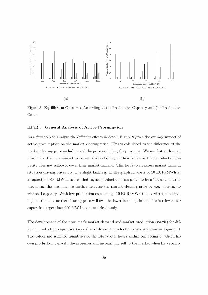
particular in the hours 9 to 14. Tables containing all supply and demand elasticities for the

6 typical days can be found in Appendix B

(a) (b)

Figure 5: Estimation Results for Price Elasticities (SU/Work): (a) Demand Elasticities, (b)

Supply Elasticities

III(i).ii Scenario Definition

We use the estimation results from above as well as market data to analyze the relationship

between price elasticities in different market situations and the role of prosumer size. There-

fore, we will first define a base scenario followed by different variations from the base scenario

that we take into account. For all scenarios we assume the prosumer’s hourly demand to

follow the pattern of the market by assigning to him 1% of overall hourly market clearing

quantities; i.e. for an hour with e.g. 40,000 MW sold on the market, the prosumer’s demand

is 400 MW. The prosumer’s average demand is approximately 550 MW, with a minimum at

375 MW and a maximum at 753 MW.

25

• Base Scenario

Figure 6 shows the development of the market prices and quantities in the 144 typical

hours. In the base scenario we assume that the production capacity of the prosumer

is close to his average hourly consumption, that is about 600 MW; and the production

costs are assumed to be close to the average market price of about 30 EUR/MWh.

Figure 6: Market Prices and Corresponding Volumes for the Typical Days

• Variations from Base Scenario

To get a better understanding of the relationship between prosumer size and costs and

optimal market behavior we want to vary on the one hand the production capacity of

the prosumer and on the other hand the production costs. For the capacity we choose

in addition different cases of capacity around the maximum hourly consumption and

minimum hourly consumption. For the production costs we choose overall five scenarios:

10 EUR/MWh and 20 EUR/MWh higher and lower than the average market price of

about 30 EUR/MWh. This is in the range of expected levelized cost of energy for

decentralized generation (see Comello & Reichelstein 2016).

With this information we can determine for every typical day and the corresponding hours

the optimal behavior of the prosumer, the corresponding “new” market price, and the profit

advantage compared to passive prosumption.

26

III(ii). Results

For each of these 30 scenarios we derived the prosumer’s optimal market behavior, i.e. market

production, market demand and self-supply. Figure 14 in Appendix D contains these optimal

values for all 4,320 typical hours (6 days times 24 hours times 30 scenarios). Here, we present

one exemplary scenario, viz. 1200/10, in Figure 7 where the x-axis depicts the 6 typical days

with their 144 hours. In most of the hours, self-supply and market production are equal to

the prosumer’s production capacity, QPSs , i.e. no capacity remains unused. The prosumer

does not cover his demand QPSd on the market and is thus a Pure Monopolist as we defined in

Case B. The market clearing price is mostly higher than the prosumer’s production costs of 10

EUR/MWh (see Figure 6); however, when these values are close, in particular in TS/Wend

and SU/Wend, we observe that the prosumer acts as a Standard Market Participant (Case

C) selling all of his production capacity on the market and at the same time covering all

of his demand on the same market. Surprisingly, maximally decreasing the market clearing

price with supply and increasing it at the same time with demand seems to be optimally in

the end. This example highlights that the prosumer’s decisions not only depend on his own

characteristics, i.e. production costs and capacity as well as demand, but also on the market

environment via different hourly demand and supply elasticities and market clearing prices.

It is, however, not clear which effect or relation is most influential. Lastly, we also observe a

negative spike of market production during a few hours in TS/Wend; self-supply and market

production do not add up to production capacity indicating that the prosumer withholds

capacity from the market, i.e. acts as a Partial Supplier (Case CD).

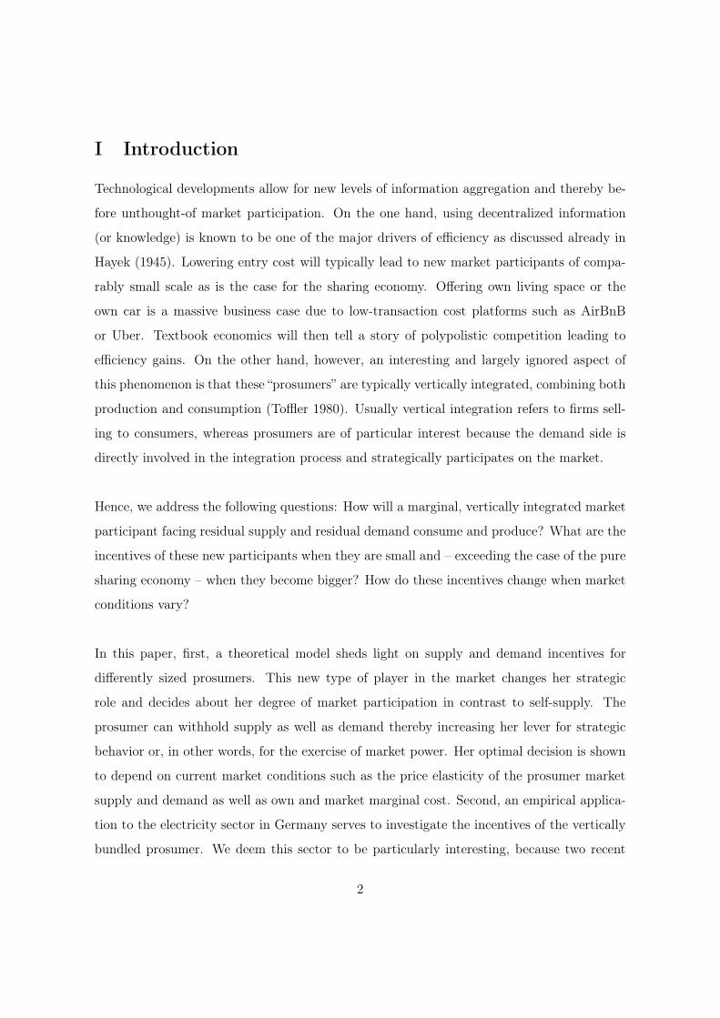
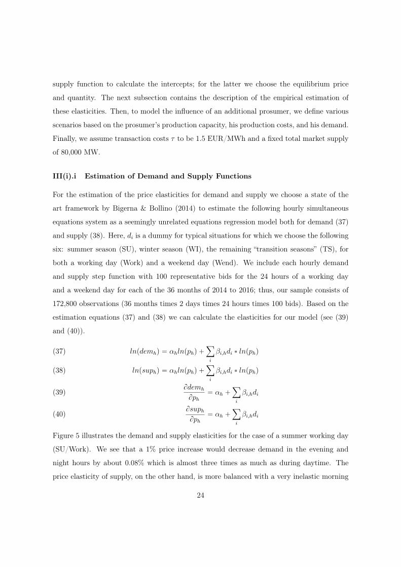
Including again all 4,320 observations hours, we proceed by classifying the results according

to the cases described in Section II(ii). above and by deriving their distribution. Figure 8

shows the frequency of the different outcomes. Part (a) on the left depicts the distribution of

cases for different production capacities, whereas Part (b) on the right shows the distributions

for different prosumer’s production costs. The values of the former are derived by calculating

e.g. for all 5 scenarios containing 200 MW of production capacity the average frequency each

case occurs. E.g. Case B occurred in all 6 different capacity scenarios on average 83 times.

27

Figure 7: Optimal Prosumer Decisions for Production Capacity of 1200 MW and Production

Costs of 10 EUR/MWh

This is done to eliminate the fourth dimension of costs and we used the same procedure for

Part (b) accordingly. Overall, Cases B (Pure Monopolist), AD (Strategic Monopsonist), and

D (Pure Monopsonist) are the most relevant ones. Part (a) indicates that choosing Case D,

i.e. being a simple consumer, is insensitive to changing production capacity. Cases B and

Case AD, on the other hand, depend strongly on the size of capacity, with the incidence

of the latter decreasing, and the former showing a maximum at 800 MW. We also see that

additional production capacity induces the prosumer to choose between more strategic cases

– 2 Cases vs. 7 Cases – because the window of attainable market clearing prices (see Figure 2)

is increased. Being able to choose only Case B or Case D is not different from being a passive

prosumer, i.e. just a small amount of production capacity does not seem to yield any profit

advantage at the first glance. In Part (b) the amount of each case appearing varies strongly

with a transition of Case B to D as costs are higher and the number of hours where costs are

larger than the market clearing price increases; i.e. the prosumer has fewer opportunities to

profitably produce for the market and switches to be a simple consumer.

28

(a) (b)

Figure 8: Equilibrium Outcomes According to (a) Production Capacity and (b) Production

Costs

III(ii).i General Analysis of Active Prosumption

As a first step to analyze the different effects in detail, Figure 9 gives the average impact of

active prosumption on the market clearing price. This is calculated as the difference of the

market clearing price including and the price excluding the prosumer. We see that with small

prosumers, the new market price will always be higher than before as their production ca-

pacity does not suffice to cover their market demand. This leads to an excess market demand

situation driving prices up. The slight kink e.g. in the graph for costs of 50 EUR/MWh at

a capacity of 800 MW indicates that higher production costs prove to be a “natural” barrier

preventing the prosumer to further decrease the market clearing price by e.g. starting to

withhold capacity. With low production costs of e.g. 10 EUR/MWh this barrier is not bind-

ing and the final market clearing price will even be lower in the optimum; this is relevant for

capacities larger than 600 MW in our empirical study.

The development of the prosumer’s market demand and market production (y-axis) for dif-

ferent production capacities (x-axis) and different production costs is shown in Figure 10.

The values are summed quantities of the 144 typical hours within one scenario. Given his

own production capacity the prosumer will increasingly sell to the market when his capacity

29

Figure 9: Average Impact on Market Clearing Price

increases. However, increasing the prosumer’s capacity relative to the total market supply

also leads to a decreasing market price which at the same time increases the prosumer’s

market demand. This can be seen in the graphs for costs of 10 and 20 EUR/MWh in Part

(a) – with the additional influence of the “outliers” of Cases C which we find in scenarios

1000/10, 1000/20, 1200/10, and 1200/20. For higher prosumer’s production costs this effect

is not likely to occur because of lacking competitiveness relative to the market. This is also

shown by the flat market production graphs for costs of 40 and 50 EUR/MWh in Part (b);

and by the flat parts of the top cost graphs in Part (a).

The observation from above, viz. that increasing production capacity leads to increased

market production, can also be visualized by plotting the ratio of residual production capacity

to total market supply, pQPSd ´QPS

s q{´Qmarkets , against the derived optimal market production

for all 4,320 observations (see Figure 11). Depending on the scenario, this ratio will be

negative if the prosumer’s hourly demand is larger than his production capacity; and as we

can see on the left side in Figure 11 the prosumer will never choose to sell any production on

the market. This ratio turns positive, on the other hand, when the prosumer’s production

capacity is larger than demand. I.e. the prosumer will only start to participate on the supply

side of the market if he owns a minimum amount of production capacity that additionally

30

(a) (b)

Figure 10: (a) Market Demand and (b) Market Production for Different PS Production Costs

and Production Capacities

exceeds his demand with the plot indicating a linear positive relationship. We can also see the

different strategic cases of the prosumer: the Cases B and D determine the outer borders of

this triangular shape; the observations in between are cases where the prosumer e.g. decides

to withhold capacity, like in Case AB. And the outliers where the prosumer offers 1000 or

1200 MW on the market are the instances of Case C.

Figure 11: Interdependence of Available Production Capacity and Market Production

31

III(ii).ii Profit Advantage of Active Prosumption

One of the results of Section II was that active prosumption is a weakly dominating strategy

and that the profit advantage depends on the relation of productions costs to market clearing

price, on the supply and demand elasticities, and on the relative size of the prosumer. Based

on our empirical study we can show this in more detail. Figure 12 shows the profits of an

excess producer, i.e. a Pure Monopolist (Case B) and of an active prosumer for all levels of

production capacity and differentiated according to production costs. The values are derived

by summing up all profits of the 144 typical hours. As capacity increases there are more and

more incidents where the prosumer can be 100% self sufficient and where excess production

will decrease the market clearing price. Part (a) shows that the Pure Monopolist’s profit can

even decline with increasing production costs because the excess production will even push

prices below costs; at some point, of course, this Pure Monopolist should choose to become

a simple consumer, i.e. a Pure Monopsonist (Case D). An active prosumer, on the other

hand, can prevent this by actively adjusting and reacting to the market environment e.g. by

withholding capacity from the market. Again, the profits are negative because we do not

take the utility of demand into account; thus the advantage of active prosumption consists

of restricting losses. In addition, we see the stated weak dominance in Part (b) for example

for costs of 20 EUR/MWh because profits are equal at low capacities, but when production

capacity increases, the active prosumer even has an additional advantage (see also Figure 11

above).

In the final Figure 13 we plot the absolute hourly profit advantages of active prosumption

for all 4,320 observations; as defined in Section II(iv). the profits of a passive prosumer are

calculated by allowing him to choose between excess production or simple consumption, i.e.

between Case B and D. We can confirm the analytical result that the advantage is highest

when the market clearing price is close to the production costs. The “peak” for costs of

10 EUR/MWh is only small as the distribution is truncated below by the observed market

clearing prices in our 144 typical hours with a minimum at 12.84 EUR/MWh. Per unit profit

increases range from 0.01 to 0.03 EUR/MWh for the smallest case of 200 MW production

32

(a) (b)

Figure 12: Sum of Profits of (a) Pure Monopolist (Case B) and (b) Active Prosumer

capacity and up to 0.03 to 2.52 EUR/MWh for the largest depicted case of 1200 MW pro-

duction capacity for different cost levels. Extending capacity up to 8700 MW enables the

prosumer to raise per unit profits from 9.7 to 13.4 EUR/MWh.

In addition, variance is higher with higher production costs. Since each set of data points

for production costs contains all six assumed production capacities, we have to resort to

the distribution of strategic cases shown in Part (a) of Figure 8 above for an explanation.

There we see that, keeping the costs constant, additional capacity increases the options for

a prosumer. Hence, we expect more production capacity to lead to a greater leeway in

strategically influencing market outcomes. This is ultimately based on the larger window

of attainable market clearing prices (see Figure 2) as production capacity increases. For

a more detailed analysis on this, we also calculated our model for a prosumer production

capacity of 8700 MW comparing to one of the largest direct sellers at current EPEXSpot,

Statkraft. We observe that this higher capacity results in the prosumer playing more the role

of a Strategic Monopolist (case AB, 22% of all situations) or a Partial Supplier (case CD,

26% of all situations). The reason for this is that bidding the total capacity into the market

would decrease the prices too much and thus decrease own profits. In contrast, the frequency

of being residual Pure Monopolist (case B) reduces, which is a consequence of increased

market power. The role Pure Monopsonist (case D) is independent of the production capacity

33

and remains at 36% of all situations. Lastly, the position of the peaks also indicates that

prosumers with different production technologies and therefore different production costs

will be active in different zones of market clearing prices. Hence, active prosumption is a

profitable strategy for all market participants who simultaneously demand from and supply

to the market.

Figure 13: Profit Advantage of Active vs. Passive Prosumption

IV Discussion

The proposed model is based on several important assumptions that need to be taken into

account for interpreting the results. First, the prosumer influences the market clearing price

by rotating both the demand and supply functions as he chooses the quantities to demand

from and supply to the market. We found that assuming a parallel shift does not change

the main results of our analysis which differ only in quantitative terms. Second, the de-

mand and supply functions are assumed to be linear, whereas in the EPEXSpot day-ahead

electricity market they are highly nonlinear (hockey-stick form) and actually step functions

with, on average, 700 steps per hour. We are able to handle this nonlinearity by estimating

the elasticities and calculating the slopes at the various market equilibria; incorporating step

functions would deprive us of the analytical analysis of an additional prosumer. Third, we

34

also assumed that the prosumer has perfect foresight of and his effect on the market clearing

price. Again regarding the electricity market, the forecasts of day-ahead prices are quite ac-

curate and, as we show in Figure 13 in Section III(ii).ii, each distribution of profit advantages

covers a range of prices; i.e. it is not necessary to perfectly know the market environment

in order to gain an advantage, it suffices to be close enough. And fourth, concerning the

profit advantage, we implicitly assume that all the 144 typical hours are equally likely to

appear during a year. We could additionally extrapolate these 144 hourly profit advantages

to e.g. an assumed typical year. This does, however, not seem meaningful as our model and

in particular the production costs are highly simplified and the additional information gained

by this exercise is unclear. We do for example not include startup costs after not using or

withholding production capacity, or ramp-up/down delays for changing the actual quantity

produced which only occur when production capacity is not simply relayed from market to

self-supply.

Several issues had to be reserved for future work. As of yet, the prosumer’s production

capacity is modeled as if it were just one unit with uniform production costs. The natural

extension would be to model a portfolio of units with different production costs each, i.e.

to a multi-unit commitment problem. Also, since active prosumption leads to a profit ad-

vantage, this business model will attract multiple active prosumers. Thus, the model must

be generalized to more than one single active prosumer in order to check for interactions or

concerted actions between these new market participants. In a next step, it is also impor-

tant to disentangle the three effects on the prosumer’s optimal decision, viz. the relation of

(a) market clearing price to production costs, (b) demand and production capacity, and (c)

elasticities.

As stated in Section III(i).i above, the elasticities indicate major prosumer action in hours

9-14 because the window of attainable prices is largest; this does, however, not include

information on the general price level, i.e. of effect (a). Finding a way to disentangle these

effects could indicate hours where we expect an increase of active prosumption. So far, we

35

only observe profit gains when production costs and market clearing prices are sufficiently

close (cf. 13). Finally, concerning active prosumption in electricity markets, the model

may be extended by including further markets, e.g. balancing market providing flexibility.

Prosumption seems to be a simple way to flexibly adapt to the market environment as, in

particular, relaying production from the market to self-supply does not involve any physical

constraints, but price signals between those markets may differ a lot changing the prosumer’s

incentives. Second, the results are based on the active prosumer’s impact on the market

clearing price, which should work even better in markets based on nodal pricing. This is

because the relative size of a prosumer as well as his impact on the price is even larger

in load pockets which occur due to transmission congestion. By comparison, our empirical

study was based on a small prosumer with only 1 % of total market demand and between

0.3 and 1.5 % of total market supply. In a further sensitivity analysis, an increase to roughly

10 % market share already led to tremendous profit gains. And lastly, an extension must

focus on giving the prosumer the possibility to intertemporally shift supply and/or demand

via storage or flexibility. Even though this is an important and very recent topic in the

electricity market – including the new term of “ProSumAge” (see Green & Staffell 2017) –

this is also important for other market environments where storing supply is possible, like

e.g. for farmers who can feed their cattle or store the grain in silos.

V Conclusion

In this article we address the important issue of consumer market participation when there is

the possibility to – at least partially – rely on marketable own production. Theoretical results

indicate that the optimal choices of production, sales and sourcing crucially depend on own

production costs and capacity as well as own demand relative to market equilibrium. We

apply our model to the electricity market. Varying scarcity situations reveal the prosumer

to switch strategic roles, from net buyer to net supplier, on an hourly basis. In particular,

the prosumer exerts market power in peak as well as off-peak situations. This is in part due

to the additional influence on market enabling her to increase market power and to substan-

36

tially increase profits even with relatively low market shares. In general, these results apply

to any market where the same participant is able to simultaneously demand from and offer

to a market having an impact on market price. The potential to either increase supply or

exert market power demonstrates the ambivalent role a prosumer can take with regard to

allocative efficiency. This also holds for other markets than electricity such as transportation

(Uber), overnight stays (AirBnB), or car-sharing markets. Further examples are Amazon’s

or Google’s server farms whose processing power may be used for their own tasks or of-

fered to other customers. This has manifold implications for assessing strategic behavior in

vertically integrated markets as well as for competition policy and regulation. Regarding

electricity markets, active prosumption is a new way for companies to vertically integrate.

This “Un-Unbundling” may serve to circumvent regulations and potentially undermine the

liberalization of the market.

37

Notes

1E.g. the Big 6 in the UK or the Big 4 in Germany compare to e.g. 150,000 private solar power systems

in Finland (TEM 2014) or to 34,000 small scale prosumer systems (including storage) in Germany.

2See Selectra (2017), innogy (2017).

3It is worth noting that active prosumption differs from other forms of market participation such as shifting

demand and/or storage (intertemporal arbitrage, see Crampes & Creti (2006), Ottesen et al. (2016)). There is

also the option of virtual bidding, which is a purely financial transaction without the actual risk of operating

a generating unit or of needing to cover physical demand. This is usually done to generate arbitrage profits

between sequential markets and the transactions must be undone again before actual delivery to or from the

virtual bidder takes place (see Jha & Wolak 2015, van Eijkel et al. 2016). We do not address these issues in

this article.

4An analysis of possible principal-agent issues and of optimal contractual design of this arrangement must

be left for future analyses.

5This is similar for other markets such as taxi rides (Uber) or overnight stays (AirBnB).

6We further assume the consumer to have an inelastic demand, therefore no optimization with respect to

consumption takes place.

7This cost can also include opportunity cost.

8Bessembinder & Lemmon (2006) find local disequilibria to provide another explanation for this phe-

nomenon. Convex cost functions in combination with locally varying demand make it profitable to hedge

throughout space and adapt real-time supply and demand locally.

9Avenel (2008) investigates the related issue of the optimal degree of vertical integration of a firm in

light of technology adoption. In contrast, this article focuses on consumer market participation based on

production by new, decentralized technologies.

10The prosumer’s effect could also be modelled as a parallel shift of both functions. Testing such a model

showed, however, that the results differ only in quantitative terms and remain the same regarding the main

points we try to make in this paper. The most realistic approach is leaving the functions unaffected up to the

“step” the prosumer introduces and introducing a parallel shift. This nonlinearity introduces many equilibria

and does again not help us forward our case.

38

A Equations for X (Optimal qPSs ) and Y (Optimal qPS

d )

The optimal hourly quantities the prosumer produces for and demands from the market, i.e.

qPSs ) and qPS

d , respectively, are derived based on Equations 4) and (5 (see Section II(ii).).

Solving the partial derivatives, setting the resulting total derivative to 0, and isolating the

respective decision variables yields the optimal (unconstrained) decision variables stated in

the equations below:

q˚,PSs “ x y

ad´ Qmarket

s ´

ba2d pad ´ asq x y pas ´ cPSq p´x y ` ad pqPS

d ` Qmarkets qq

a2d pas ´ cPSq

q˚,PSd “ ad z

x´ Qmarket

d `

bad pad ´ asq x2 z pad ´ cPS ` ⌧q p´ x pqPS

s ` Qmarketd q ` ad zq

x2 pad ´ cPS ` ⌧qwhere

x “ as ´ cmarket

y “ qPSd ` Qmarket

d

z “ qPSs ` Qmarket

s

39

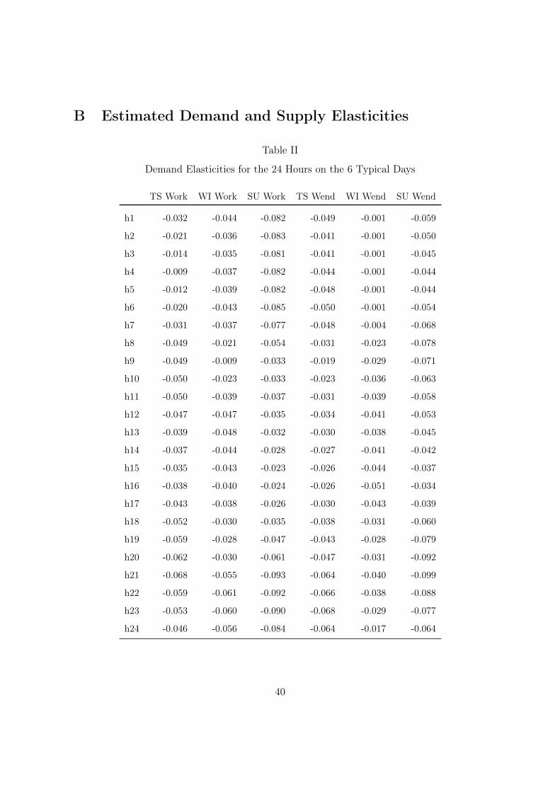
B Estimated Demand and Supply Elasticities

Table II

Demand Elasticities for the 24 Hours on the 6 Typical Days

TS Work WI Work SU Work TS Wend WI Wend SU Wend

h1 -0.032 -0.044 -0.082 -0.049 -0.001 -0.059

h2 -0.021 -0.036 -0.083 -0.041 -0.001 -0.050

h3 -0.014 -0.035 -0.081 -0.041 -0.001 -0.045

h4 -0.009 -0.037 -0.082 -0.044 -0.001 -0.044

h5 -0.012 -0.039 -0.082 -0.048 -0.001 -0.044

h6 -0.020 -0.043 -0.085 -0.050 -0.001 -0.054

h7 -0.031 -0.037 -0.077 -0.048 -0.004 -0.068

h8 -0.049 -0.021 -0.054 -0.031 -0.023 -0.078

h9 -0.049 -0.009 -0.033 -0.019 -0.029 -0.071

h10 -0.050 -0.023 -0.033 -0.023 -0.036 -0.063

h11 -0.050 -0.039 -0.037 -0.031 -0.039 -0.058

h12 -0.047 -0.047 -0.035 -0.034 -0.041 -0.053

h13 -0.039 -0.048 -0.032 -0.030 -0.038 -0.045

h14 -0.037 -0.044 -0.028 -0.027 -0.041 -0.042

h15 -0.035 -0.043 -0.023 -0.026 -0.044 -0.037

h16 -0.038 -0.040 -0.024 -0.026 -0.051 -0.034

h17 -0.043 -0.038 -0.026 -0.030 -0.043 -0.039

h18 -0.052 -0.030 -0.035 -0.038 -0.031 -0.060

h19 -0.059 -0.028 -0.047 -0.043 -0.028 -0.079

h20 -0.062 -0.030 -0.061 -0.047 -0.031 -0.092

h21 -0.068 -0.055 -0.093 -0.064 -0.040 -0.099

h22 -0.059 -0.061 -0.092 -0.066 -0.038 -0.088

h23 -0.053 -0.060 -0.090 -0.068 -0.029 -0.077

h24 -0.046 -0.056 -0.084 -0.064 -0.017 -0.064

40

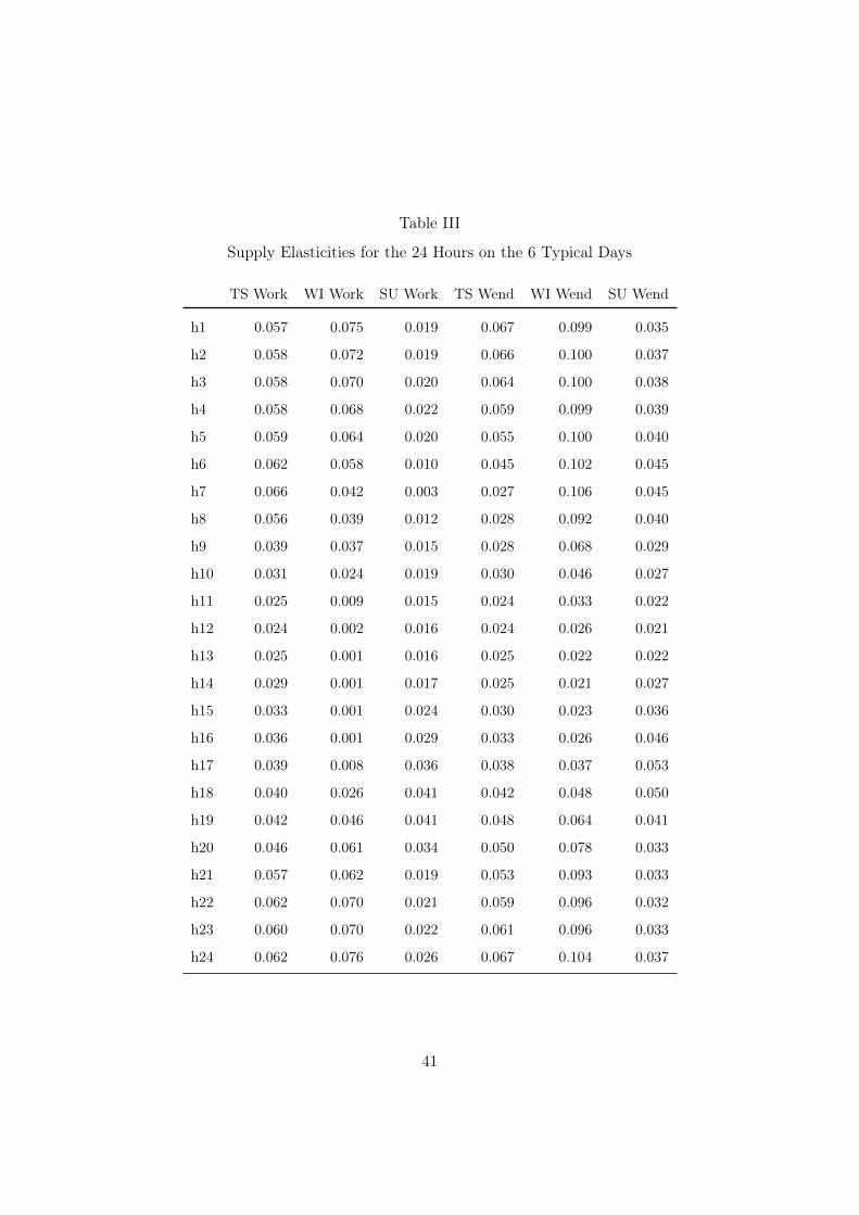
Table III

Supply Elasticities for the 24 Hours on the 6 Typical Days

TS Work WI Work SU Work TS Wend WI Wend SU Wend

h1 0.057 0.075 0.019 0.067 0.099 0.035

h2 0.058 0.072 0.019 0.066 0.100 0.037

h3 0.058 0.070 0.020 0.064 0.100 0.038

h4 0.058 0.068 0.022 0.059 0.099 0.039

h5 0.059 0.064 0.020 0.055 0.100 0.040

h6 0.062 0.058 0.010 0.045 0.102 0.045

h7 0.066 0.042 0.003 0.027 0.106 0.045

h8 0.056 0.039 0.012 0.028 0.092 0.040

h9 0.039 0.037 0.015 0.028 0.068 0.029

h10 0.031 0.024 0.019 0.030 0.046 0.027

h11 0.025 0.009 0.015 0.024 0.033 0.022

h12 0.024 0.002 0.016 0.024 0.026 0.021

h13 0.025 0.001 0.016 0.025 0.022 0.022

h14 0.029 0.001 0.017 0.025 0.021 0.027

h15 0.033 0.001 0.024 0.030 0.023 0.036

h16 0.036 0.001 0.029 0.033 0.026 0.046

h17 0.039 0.008 0.036 0.038 0.037 0.053

h18 0.040 0.026 0.041 0.042 0.048 0.050

h19 0.042 0.046 0.041 0.048 0.064 0.041

h20 0.046 0.061 0.034 0.050 0.078 0.033

h21 0.057 0.062 0.019 0.053 0.093 0.033

h22 0.062 0.070 0.021 0.059 0.096 0.032

h23 0.060 0.070 0.022 0.061 0.096 0.033

h24 0.062 0.076 0.026 0.067 0.104 0.037

41

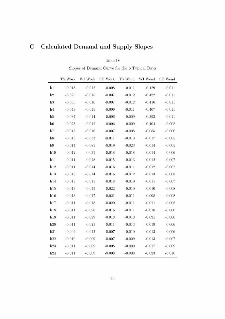
C Calculated Demand and Supply Slopes

Table IV

Slopes of Demand Curve for the 6 Typical Days

TS Work WI Work SU Work TS Wend WI Wend SU Wend

h1 -0.018 -0.012 -0.008 -0.011 -0.429 -0.011

h2 -0.025 -0.015 -0.007 -0.012 -0.422 -0.011

h3 -0.035 -0.016 -0.007 -0.012 -0.416 -0.011

h4 -0.049 -0.015 -0.006 -0.011 -0.407 -0.011

h5 -0.037 -0.014 -0.006 -0.009 -0.393 -0.011

h6 -0.023 -0.012 -0.006 -0.009 -0.404 -0.008

h7 -0.018 -0.016 -0.007 -0.008 -0.085 -0.006

h8 -0.013 -0.033 -0.011 -0.013 -0.017 -0.005

h9 -0.014 -0.085 -0.019 -0.023 -0.014 -0.005

h10 -0.012 -0.031 -0.018 -0.018 -0.014 -0.006

h11 -0.011 -0.018 -0.015 -0.013 -0.012 -0.007

h12 -0.011 -0.014 -0.016 -0.011 -0.012 -0.007

h13 -0.013 -0.014 -0.016 -0.012 -0.013 -0.008

h14 -0.013 -0.015 -0.018 -0.010 -0.011 -0.007

h15 -0.013 -0.015 -0.022 -0.010 -0.010 -0.008

h16 -0.013 -0.017 -0.021 -0.011 -0.008 -0.008

h17 -0.011 -0.018 -0.020 -0.011 -0.011 -0.008

h18 -0.011 -0.026 -0.016 -0.011 -0.018 -0.006

h19 -0.011 -0.029 -0.013 -0.013 -0.021 -0.006

h20 -0.011 -0.025 -0.011 -0.013 -0.019 -0.006

h21 -0.009 -0.012 -0.007 -0.010 -0.013 -0.006

h22 -0.010 -0.009 -0.007 -0.009 -0.013 -0.007

h23 -0.011 -0.009 -0.008 -0.009 -0.017 -0.009

h24 -0.011 -0.009 -0.008 -0.008 -0.023 -0.010

42

Table V

Slopes of Supply Curves for the 6 Typical Days

TS Work WI Work SU Work TS Wend WI Wend SU Wend

h1 0.010 0.007 0.033 0.008 0.005 0.018

h2 0.009 0.008 0.032 0.008 0.004 0.015

h3 0.009 0.008 0.028 0.008 0.004 0.013

h4 0.008 0.008 0.024 0.008 0.004 0.012

h5 0.008 0.008 0.026 0.008 0.004 0.012

h6 0.007 0.009 0.049 0.010 0.004 0.009

h7 0.008 0.014 0.186 0.015 0.003 0.009

h8 0.012 0.018 0.051 0.014 0.004 0.010

h9 0.017 0.020 0.042 0.015 0.006 0.013

h10 0.019 0.030 0.031 0.014 0.011 0.015

h11 0.022 0.077 0.035 0.016 0.015 0.017

h12 0.022 0.347 0.034 0.016 0.020 0.018

h13 0.019 0.658 0.031 0.015 0.021 0.017

h14 0.016 0.656 0.029 0.011 0.021 0.012

h15 0.014 0.656 0.021 0.009 0.018 0.008

h16 0.013 0.669 0.017 0.009 0.016 0.006

h17 0.013 0.085 0.014 0.008 0.012 0.006

h18 0.014 0.030 0.014 0.010 0.012 0.008

h19 0.015 0.017 0.015 0.011 0.010 0.012

h20 0.015 0.012 0.020 0.013 0.007 0.018

h21 0.011 0.011 0.035 0.011 0.006 0.019

h22 0.010 0.008 0.032 0.010 0.005 0.020

h23 0.010 0.008 0.032 0.010 0.005 0.022

h24 0.008 0.007 0.025 0.008 0.004 0.017

43

D Summary of Optimal Prosumer Decisions

Figure 14: Optimal PS Decisions for 4,320 Typical Hours

44

References

Avenel, E. (2008), ‘Strategic Vertical Integration Without Foreclosure’, The Journal of In-

dustrial Economics 55(2), 247–262.

Bessembinder, H. & Lemmon, M. (2002), ‘Equilibrium pricing and optimal hedging in elec-

tricity forward markets’, Journal of Finance 57, 1347–1382.

Bessembinder, H. & Lemmon, M. (2006), ‘Gains from Trade under Uncertainty: The Case

of Electric Power Markets’, The Journal of Business 79(1), 1755–1782.

Bigerna, S. & Bollino, C. A. (2014), ‘Electricity Demand in Wholesale Italian Market’, The

Energy Journal 35(3), 25–46.

BMJ (2017), ‘Gesetz für den Ausbau ernerubarer Energien, EEG 2017’.

URL: https://www.gesetze-im-internet.de/eeg_2014/BJNR106610014.html

Boom, A. (2009), ‘Vertically integrated firms’ investments in electricity generating capacities’,

International Journal of Industrial Organization 27(4), 544–551.

Borenstein, S., Bushnell, J. & Wolak, F. (2002), ‘Measuring Market Inefficiencies in

California’s Restructured Wholesale Electricity Market’, American Economic Review

92(5), 1376–1405.

Bresnahan, T. F. & Levin, J. D. (2012), ‘Vertical Integration and Market Structure’, NBER

Working Paper Series 17889.

Bushnell, J. B., Mansur, E. T. & Saravia, C. (2008), ‘Vertical Arrangements, Market Struc-

ture, and Competition : An Analysis of Restructured US Electricity Markets’, American

Economic Review 98(1), 237–266.

Comello, S. D. & Reichelstein, S. J. (2016), ‘The U.S. Investment Tax Credit for Solar

Energy: Alternatives to the Anticipated 2017 Step-Down’, Renewable and Sustainable

Energy Reviews 55, 591–602.

45

Crampes, C. & Creti, A. (2006), ‘Capacity Competition in Electricity Markets’, Economia

delle fonti di energia e dell’ambiente 48(2), 59–83.

EC (2007), ‘Third Package on Energy Market Legislation’. European Commission,

2009/72/EC.

Green, R. & Staffell, I. (2017), ‘Prosumage and the British electricity market’, Economics of

Energy & Environmental Policy 6(1), 33–49.

Hanna, R., Ghonima, M., Kleissl, J., Tynan, G. & Victor, D. G. (2017), ‘Evaluating business

models for microgrids: Interactions of technology and policy’, Energy Policy 103, 47–61.

Hastings, J. S. & Gilbert, R. J. (2005), ‘Market Power, Vertical Integration and the Wholesale

Price of Gasoline’, The Journal of Industrial Economics 53(4), 469–492.

Hayek, F. A. (1945), ‘The Use of Knowledge in Society’, American Economic Review

35(4), 519–530.

IEA Wind (2015), ‘Annual report’.

URL: https://www.ieawind.org/annual_reports_PDF/2015.html

innogy (2017), ‘Fuer Zuhause. Energie selbst erzeugen. Lass die Sonne rein. Photovoltaik -

aus Sonne wird Strom.’.

URL: https://www.innogy.com/web/cms/de/3700364/fuer-zuhause/

energie-selbst-erzeugen/lass-die-sonne-rein/photovoltaik-lohnt-sich/?etcc_cmp=

kampagne_solar_032017\%2B&etcc_med=STC_CC_ATTR_VALUE_OTHER&

etcc_var=tsr_Photovoltaik-lohnt-sich\&etcc_cu=onsite

IRENA (2016), ‘Solar photovoltaics’.

URL: https://www.irena.org/DocumentDownloads/Publications/RE_Technologies_

Cost_Analysis-SOLAR_PV.pdf

Jha, A. & Wolak, F. A. (2015), ‘Testing for market efficiency with transaction costs: An

application to financial trading in wholesale electricity markets’.

URL: https://web.stanford.edu/group/fwolak/cgi-bin/?q=node/3

46

Joskow, P. L. (2010), ‘Vertical Integration’, Antitrust Bulletin 55(3), 545–586.

Joskow, P. & Tirole, J. (2007), ‘Reliability and competitive electricity markets’, RAND Jour-

nal of Economics 38(1), 60–84.

Kairies, K.-P., Haberschusz, D., Ouwerkerk, J. v., Strebel, J., Wessels, O., Magnor, D.,

Badeda, J. & Sauer, D. U. (2016), ‘Wissenschaftliches Mess- und Evaluierungsprogramm

Solarstromspeicher’. RWTH Aachen, Aachen, Germany.

URL: http://www.speichermonitoring.de/fileadmin/user_upload/Speichermonitoring_

Jahresbericht_2016_Kairies_web.pdf

Longstaff, F. & Wang, A. (2004), ‘Electricity Forward Prices: A High-Frequency Empirical

Analysis’, Journal of Finance 59(4), 1877–1900.

Mansur, E. T. (2007), ‘Upstream Competition and Vertical Integration in Electricity Mar-

kets’, Journal of Law and Economics 50, 125–156.

Ordover, J., Saloner, G. & Salop, S. (1990), ‘Equilibrium Vertical Foreclosure’, American

Economic Review 80(1), 127–142.

Ottesen, S., Tomasgard, A. & Fleten, S.-E. (2016), ‘Prosumer bidding and scheduling in

electricity markets’, Energy 94, 828–843.

Rigo-Mariani, R., Sareni, B., Roboam, X. & Turpin, C. (2014), ‘Optimal power dispatching

strategies in smart-microgrids with storage’, Renewable and Sustainable Energy Reviews

40, 649–658.

Riordan, M. (1998), ‘Anticompetitive Vertical Integration by a Dominant Firm’, American

Economic Review 88(5), 1232–1248.

Riordan, M. (2008), ‘Competitive Effects of Vertical Integration’, Handbook of Antitrust

Economics, ed. by P. Buccirossi, MIT Press pp. 145–182.

Salinger, M. (1988), ‘Vertical Mergers and Market Foreclosure’, The Quarterly Journal of

Economics 103(2), 345–356.

47

Schill, W.-P., Zerrahn, A. & Kunz, F. (2017), ‘Prosumage of solar electricity: pros, cons, and

the system perspective’, Economics of Energy & Environmental Policy 6(1), 7–31.

Selectra (2017), ‘Einspeisetarife fuer Photovoltaik-Kunden in Oesterreich’.

URL: http://stromliste.at/nuetzliche-infos/pv-anlagen/einspeisetarife

Shirazi, E. & Jadid, S. (2017), ‘Cost reduction and peak shaving through domestic load

shifting and DERs’, Energy 124, 146–159.

Spiegel, Y. (2013), ‘Backward integration, forward integration, and ver-

tical foreclosure’, Working Paper retrieved 1st of Jan 2018 on URL:

https://www.tau.ac.il/ spiegel/papers/foreclose-Aug-16-2013.pdf .

Toffler, A. (1980), The third wave, William Morrow, New York, NY.

Töpfer, K., Adigbli, P. & Martin, A. (2017), ‘Direktvermarktung von erneuerbaren Energien

an der Strombörse. Ein deutsch-französischer Erfahrungsbericht zur Marktintegration von

erneuerbaren Energien’.

URL: http://www.epexspot.com/de/presse/press-archive/details/press/

Direktvermarktung_wirkt_

van Eijkel, R., Kuper, G. H. & Moraga-González, J. L. (2016), ‘Do firms sell forward for

strategic reasons? An application to the wholesale market for natural gas’, International

Journal of Industrial Organization 49(1), 1–35.

Wolak, F. (2003), ‘Measuring Unilateral Market Power in Wholesale Electricity Markets:

The California Market’, AEA Papers and Proceedings 93(2), 425–30.

48