Int J Comput Vis (2009) 83: 211–232DOI 10.1007/s11263-009-0216-2

Shape Based Detection and Top-Down Delineation Using ImageSegments

Lena Gorelick · Ronen Basri

Received: 5 May 2008 / Accepted: 16 January 2009 / Published online: 27 February 2009© Springer Science+Business Media, LLC 2009

Abstract We introduce a segmentation-based detection andtop-down figure-ground delineation algorithm. Unlike com-mon methods which use appearance for detection, ourmethod relies primarily on the shape of objects as is re-flected by their bottom-up segmentation.

Our algorithm receives as input an image, along withits bottom-up hierarchical segmentation. The shape of eachsegment is then described both by its significant boundarysections and by regional, dense orientation information de-rived from the segment’s shape using the Poisson equation.Our method then examines multiple, overlapping segmenta-tion hypotheses, using their shape and color, in an attemptto find a “coherent whole,” i.e., a collection of segments thatconsistently vote for an object at a single location in the im-age. Once an object is detected, we propose a novel pixel-level top-down figure-ground segmentation by “competitivecoverage” process to accurately delineate the boundaries ofthe object. In this process, given a particular detection hy-pothesis, we let the voting segments compete for interpreting(covering) each of the semantic parts of an object. Incorpo-rating competition in the process allows us to resolve ambi-guities that arise when two different regions are matched tothe same object part and to discard nearby false regions thatparticipated in the voting process.

We provide quantitative and qualitative experimental re-sults on challenging datasets. These experiments demon-strate that our method can accurately detect and segment

L. Gorelick (�)Dept. of Computer Science and Applied Mathematics, WeizmannInstitute of Science, Rehovot 76100, Israele-mail: lena.gorelick@weizmann.ac.il

R. BasriToyota Technological Institute at Chicago, Chicago, IL 60637,USA

objects with complex shapes, obtaining results compara-ble to those of existing state of the art methods. Moreover,our method allows us to simultaneously detect multiple in-stances of class objects in images and to cope with challeng-ing types of occlusions such as occlusions by a bar of vary-ing size or by another object of the same class, that are dif-ficult to handle with other existing class-specific top-downsegmentation methods.

Keywords Shape-based object detection · Class-basedtop-down segmentation

1 Introduction

We present a segmentation-based system for detection andfigure-ground delineation. Unlike many other methods, seeSect. 2, which use appearance for detection, our methodrelies primarily on the shape of objects, as is reflected bytheir (bottom-up) segmentation in the image. Shape infor-mation, available in the image in the form of coherent im-age regions/segments and their bounding contours, providesa powerful cue that can be used for detection and segmen-tation of objects under a variety of lighting conditions andin the presence of significant deformations. While the ro-bust extraction of adequate shape information for recogni-tion still poses a considerable challenge, recent advancesin recognition allow rapid examination of partial shape hy-potheses. Statistical tests can then evaluate ensembles ofsuch hypotheses and identify the presence of objects of in-terest in the image.

In order to utilize shape for recognition we need to iden-tify three main components: (1) a method for extractionof shape hypotheses from images, (2) a representation of

212 Int J Comput Vis (2009) 83: 211–232

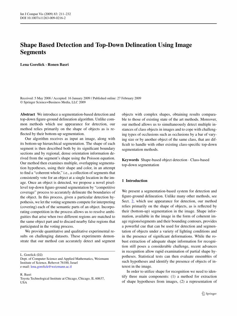
Fig. 1 (a) An input image, (b) its voting map (overlaid on the originalinput image), and (c) top-down segmentations for the detected objecthypotheses. Each hypothesis is marked with a different color. The

brighter the color is at a pixel the higher the confidence is in assigningthe pixel to the foreground of that particular hypothesis

shapes to be applied to both database shape model and im-age shapes, and (3) a method for comparing these represen-tations for recognition.

Image segmentation provides a natural means for extract-ing shape hypotheses. However, since in general existingimage segmentation algorithms cannot reliably extract com-plete objects from an image, we rely on a hierarchical seg-mentation to provide overlapping partial shape hypotheses.Moreover, to account for over-segmentations, which mayoccur at intermediate levels of the segmentation hierarchy,our shape representation is designed to rely mainly on thesignificant (sharp) boundary sections of the segment. Theseare the locations in the underlying image where sharp tran-sition in color/texture takes place and therefore they conveyuseful shape information.

We represent shape using two types of local descriptors.The first type encodes the boundaries of the shape. The sec-ond type is a regional descriptor, which includes a denselocal orientation field derived from the shape by solving aPoisson equation on the shape. We augment this represen-tation by storing in addition a color histogram with eachshape.

These shape descriptors are used to compare the seg-ments extracted from the image to a database of object sil-houettes stored in memory. Partial matches then vote for po-tential object locations. Our voting scheme uses the princi-ples outlined in Leibe et al. (2008), but utilizes segments ofdifferent sizes and shapes in the voting process. Once an ob-ject is detected, we propose a novel competitive coverageprocess to accurately delineate the boundaries of the object.In this process the voting segments compete for interpret-ing (covering) each of the semantic parts of an object. Ouraim in this process is not only to identify the regions in theimage that voted for the object, but also to resolve ambi-guities that arise when two different regions are matched tothe same model part and to discard nearby false regions thatparticipated in the voting process.

Figure 1 shows an example of a challenging input im-age along with its voting map and top-down segmentationscomputed with our method. Note that this image containsmultiple object instances, some of which are substantiallyoccluded and/or significantly vary in scale.

We provide quantitative experimental results by apply-ing our method to two challenging horse and skate-runnerdatasets. These experiments demonstrate that our method iscapable of accurately detecting and segmenting objects withcomplex shapes even with as few as ten training examples.While obtaining results comparable to those of existing stateof the art methods on images with a single object instance,our method allows us to simultaneously detect multiple in-stances of class objects in images and to cope with chal-lenging types of occlusions that are difficult to handle withother existing class-specific top-down segmentation meth-ods. To demonstrate this we perform further qualitative testsand show detection maps and top-down segmentations com-puted for a number of difficult out-of-dataset images con-taining multiple instances of horses and skate-runners andsevere occlusions of various types (see discussion and fig-ures in Sect. 4.3).

The remainder of the paper is divided as follows. Sec-tion 2 places our approach in the context of other relatedwork. Our approach is described in detail in Sect. 3. Exper-imental results are shown in Sect. 4.

2 Related Work

The success of early work, which approached recognitionusing both independent collections and dependent constel-lations of local appearances (Burl et al. 1998; Weber et al.2000; Ullman et al. 2001; Agarwal and Roth 2002), led to asurge of studies that explored different aspects of the prob-lem. Here we only briefly mention a few. Common to mostof this work is the use of local descriptors (e.g., raw in-tensity patches (Ullman et al. 2001; Vidal-Naquet and Ull-man 2003; Agarwal and Roth 2002; Leibe et al. 2008), lo-cal filter responses (Felzenszwalb and Huttenlocher 2005;Pantofaru et al. 2008), local edge elements and/or their de-scriptors (Kumar et al. 2004; Mori et al. 2004; Shotton etal. 2005; Ren et al. 2005b; Opelt et al. 2006; Ferrari et al.2007; Wang et al. 2007), and small regions obtained by over-segmentation (Ren et al. 2005a; Pantofaru et al. 2008; Caoand Fei-Fei 2007), and the reliance on a statistical model to

Int J Comput Vis (2009) 83: 211–232 213

relate these descriptions to a coherent shape. Such an ap-proach has the advantage that it requires only minimal pre-processing of the image, and so it is less sensitive to errorsthat may result from such preprocessing.

The position we take in this paper is that larger regionsidentified in the image as a result of a grouping process(bottom-up segmentation), can nevertheless provide elabo-rate shape information which is less affected by variationsin the color, texture and lighting conditions present in theimage and hence may be useful for recognition. Moreover,while segmentations essentially encode the same informa-tion as edge elements, they may give rise to sparser setsof boundaries whenever a relatively coarse segmentation isconsidered, allowing to reduce the number of object hy-potheses to be evaluated in the detection stage. Finally, co-herent image regions emerging from a bottom-up segmen-tation can be used by top-down processes to delineate fore-ground regions that are consistent with the boundaries in theimage.

Several recent methods use bottom-up segmentations fordiscovering object and scene categories. The impressivemethod of Todorovic and Ahuja (2007) uses co-occurrence,similarity and clustering of hierarchical bottom-up segmen-tation sub-trees to unsupervisely learn the taxonomy of vi-sual categories present in images. In the method of Wang etal. (2007) top-down object hypotheses are refined by align-ing them to any feasible bottom-up segmentation of the in-put image. The method of Borenstein (2006) constructs aBayesian model that integrates top-down with bottom-upsegmentations to obtain figure-ground class-specific objectsegmentation. The method of Russell et al. (2006) uses mul-tiple segmentations of each image to increase the chance ofobtaining a few “good” segments that will contain potentialobjects, while each segment is assumed to be a potential ob-ject in its entirety. The method of Cao and Fei-Fei (2007)applies to a single level segmentation (over-segmentation)and uses the over-segmented pieces as building blocks fortheir hierarchical model. The methods of both Russell etal. (2006) and Cao and Fei-Fei (2007) describe image re-gions using visual “bag of words” (capturing mostly the ap-pearance of objects) and rely on probabilistic latent seman-tic analysis (pLSA) to simultaneously recognize categoriesof objects in images. In contrast to that, our method doesnot rely on robustness and reproducibility of the segmenta-tion structure for different objects of the same class, nor onextracting visual appearance features, but rather on denseregional shape representation of objects exemplars and thesegments themselves. Such a representation is less affectedby variations in the appearance of the objects belonging tothe same class and is suitable for recognition of objects withdistinctive shapes.

The system we present also combines and modifies sev-eral existing components:

• We use segmentations obtained with the method of Sharonet al. (2006). This method provides in one pass a completehierarchical decomposition of the image into segments byapplying a process of recursive coarsening, in which thesame minimization problem is represented with fewer andfewer variables producing an irregular pyramid. Duringthis coarsening process the algorithm generates and com-bines multiscale measurements of intensity contrast andtexture differences, giving rise to regions that differ byfine as well as coarse properties with accurately locatedboundaries. We extend the segmentation algorithm aboveto cope with color images.

It is worth noting, however, that our method is not lim-ited to any particular type of segmentation algorithm aslong as it is hierarchical.

• Poisson equation was proposed in Gorelick et al. (2006) tocharacterize the shape of pre-segmented complete silhou-ettes. The solution to the Poisson equation at a point in-ternal to the silhouette represents the mean time requiredfor a particle undergoing a random walk starting at a pointto hit the boundary (see Sect. 3.1.2 and Fig. 5(b)). Sucha representation allows to smoothly propagate the con-tour information of a silhouette to every pixel internalto the silhouette resulting in a dense shape representa-tion. In practice, bottom-up segmentation algorithms of-ten fail to extract complete object silhouettes. Therefore,unlike Gorelick et al. (2006), our method applies to par-tial silhouettes (shapes) formed by segments at interme-diate scales of the bottom-up segmentation, possibly withincomplete boundaries. To reduce the effect of the miss-ing boundary sections on the computed shape descriptorswe modify the Poisson equation in Gorelick et al. (2006)by introducing mixed Dirichlet and Neumann boundaryconditions (see Sect. 3.1.2).

• For detection we use probabilistic voting that follows theprinciples proposed in Leibe et al. (2008). Our votingscheme, however, differs in several important respects.First, as opposed to rectangular intensity patches in Leibeet al. (2008), our voting scheme applies to segments ofdifferent sizes and shapes, characterized by dense localshape properties. Second, the segments are matched toa database model, characterized by similar local shapeproperties, rather than a code book of rectangular appear-ance patches. Finally, segments emerging from a bottom-up segmentation provides a natural way for object delin-eation consistent with the boundaries present in the im-age.

The problem of class specific segmentations was ad-dressed in several papers (Borenstein et al. 2004; Ku-mar et al. 2005; Winn and Jojic 2005; Levin and Weiss2006; Wang et al. 2007; Borenstein 2006; Leibe et al.2008), in many cases independent of detection. These stud-ies further demonstrate the potential benefits of combining

214 Int J Comput Vis (2009) 83: 211–232

bottom-up with top-down information. Some of these ap-proaches (Borenstein et al. 2004; Borenstein 2006) use im-age segmentation to guide top-down figure-ground delin-eation. However, they rely primarily on intensity fragmentsfor the detection phase. Once an object is detected (Boren-stein et al. 2004; Borenstein 2006) seek consistent place-ments of the voting fragments with the results of bottom-upsegmentation. Moreover, these approaches do not constrainthe relative location of object parts in the detection phase.In contrast to these studies, our method does not use in-tensity patches but relies exclusively on shape descriptionsobtained from the bottom-up segmentation. In addition, therelative location of parts plays a significant role in the detec-tion phase.

Generally in studies that address the problem of class-specific image segmentation, image pixels are classified aseither foreground or background based directly on the votescast by patches containing the pixels (see, e.g., Leibe et al.2008). Below we propose a new, top-down segmentationmethod by competitive coverage. In our scheme we let thevoting segments compete for interpreting the same semantic

area of an object. We then choose the most likely segment toexplain each part, yielding sharper delineation than that ob-tained by directly applying (Leibe et al. 2008) to segments,(see discussion in Sect. 3.3 and examples in Sect. 4).

3 Approach

In the following section we describe our detection and thetop-down segmentation approach.

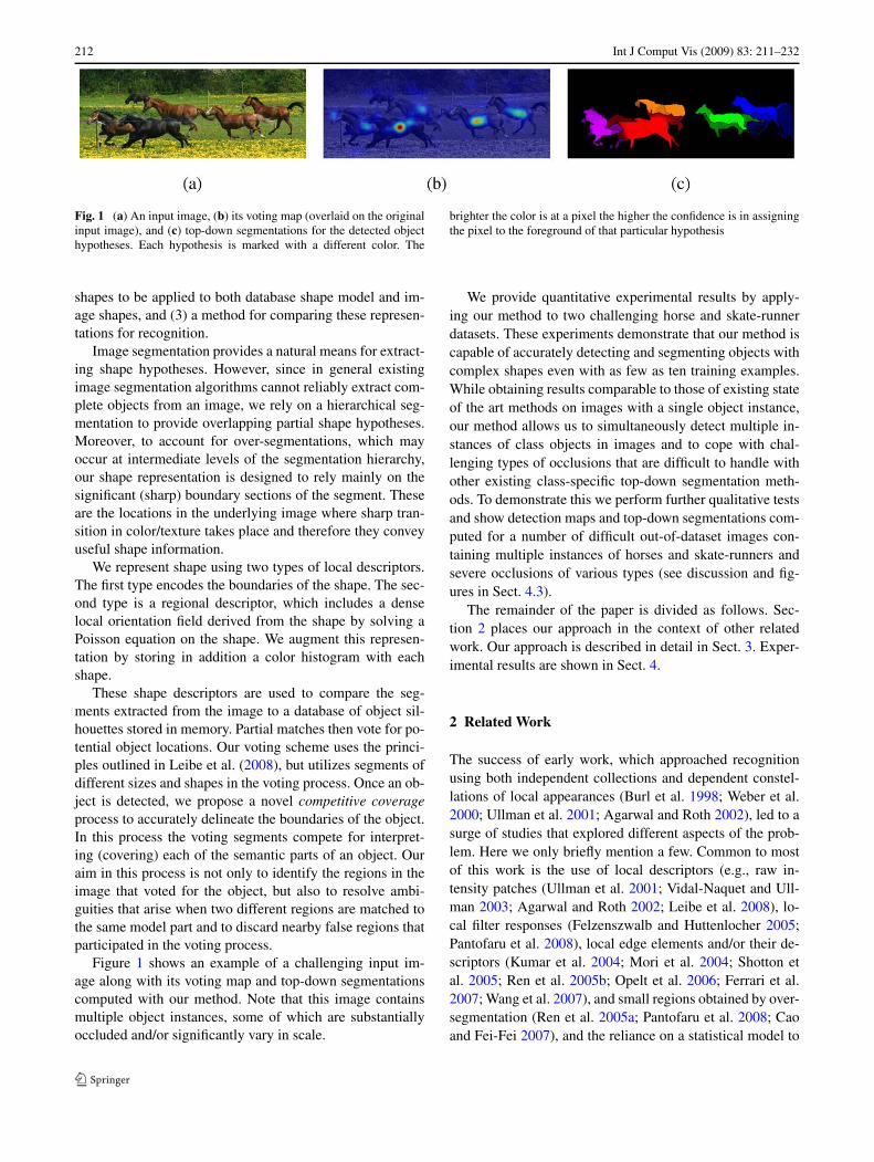
The main components of our detection algorithm areshown graphically in Fig. 2. Our algorithm receives as in-put an image in (a), along with its hierarchical segmenta-tion in (b). We use segmentations obtained with the methodof Sharon et al. (2006). This method gradually mergessegments according to criteria based on intensity and tex-ture, providing segmentation maps at several scales contain-ing segments of different shapes and sizes. We extend thismethod to cope with color images by applying all its arse-nal of multiscale measurements in a transformed HSV colorspace (tHSV) defined by (vs cosh,vs sinh,v) for a particu-lar (h, s, v) value.

Fig. 2 Given an input image in (a), and its hierarchical segmentationin (b), each segment is matched to a database of object silhouette ex-emplars in (d) based on its shape information, namely, boundary and

regional (interior) representation in (c) to obtain a set of segment inter-pretations in (e). Each interpretation then votes for a potential objectlocation in a probabilistic framework, resulting in voting map in (f)

Int J Comput Vis (2009) 83: 211–232 215

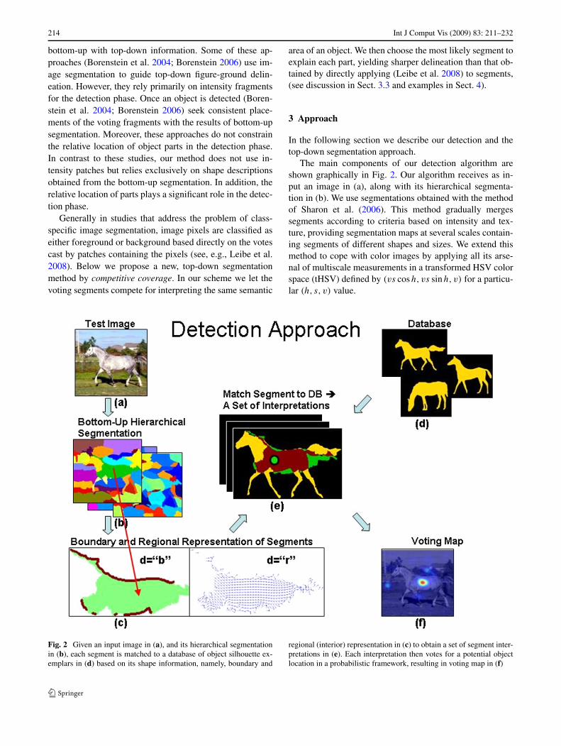
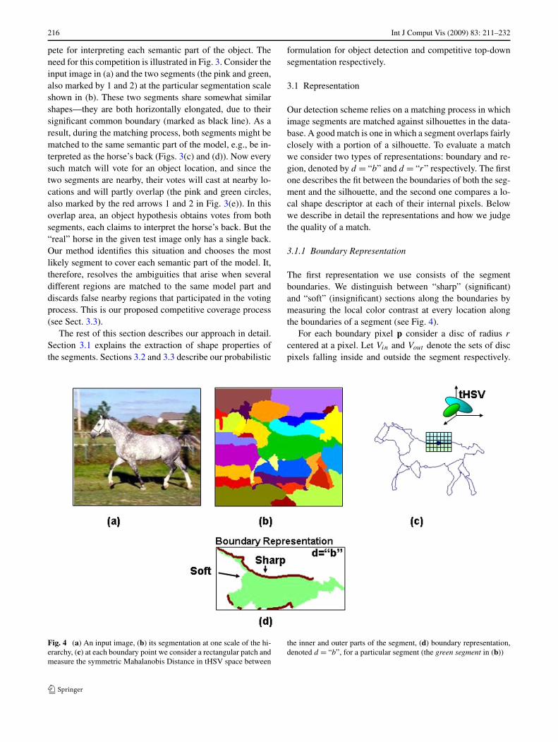
Fig. 3 Top-down, figure-ground segmentation: the need for a com-petitive coverage process. (a) An input image, (b) its hierarchicalsegmentation and an example of two neighboring segments (pink andgreen also marked by 1 and 2 for clarity) sharing a significant com-mon boundary (marked in black). (c, d) The above two segments arematched to the database of silhouette exemplars to activate twointer-pretations (both as horses’s back) along with the relative object centers

(marked by the pink and green circles accordingly). (e) A voting mapbased solely on the votes of the above two interpretations (markedby the blue and green circles). Both segments contributed to the hy-pothesis in the overlap area (marked by the black arrow) while beinginterpreted as horse’s back, but the “real” horse in the input image has asingle back

For each segment we then maintain its boundaries, whileidentifying the sections where sharp transitions in color ortexture occur. These boundary sections convey useful shapeinformation, and therefore are considered as significant or“sharp”. Figure 2(c) shows an example of an image seg-ment along with its boundary representation. The signifi-cant (“sharp”) portions of its boundaries are marked in red.(See Sect. 3.1.1 for more details.) We further store regionalproperties computed by solving a Poisson equation on thesegment. This descriptor assigns to each internal pixel thelocal orientation of the segment near that pixel. Figure 2(c)shows an example of a segment along with its regional rep-resentation (local orientation at every pixel is representedby small arrows). Note that all the body pixels are assignedwith horizontal orientation of the body, while the pixelsnear the neck region show diagonal orientation of the neck.(See Sect. 3.1.2 for more details.) Using these properties

we match each segment to a model of an object class rep-resented by a collection of segmented silhouette exemplarsstored in memory (shown in Fig. 2(d)), characterized bysimilar local shape properties, to activate a set of interpre-tations (shown in Fig. 2(e)). By interpretation we mean theeffective part of a database model (silhouette) that was ex-plained by the segment match, e.g., pixels of the back, leg orhead lying in the overlap area (the segment is green, the data-base model is yellow and the overlap/match area is brown).Each activated interpretation augmented with the color in-formation of its pixels votes for an object and its center lo-cation resulting in a voting map (shown in Fig. 2(f)). Ob-ject hypotheses are then found as local maxima in the votingspace.

Finally, for a given object hypothesis we apply a pixel-level figure-ground top-down segmentation process by“competitive coverage” in which the voting segments com-

216 Int J Comput Vis (2009) 83: 211–232

pete for interpreting each semantic part of the object. Theneed for this competition is illustrated in Fig. 3. Consider theinput image in (a) and the two segments (the pink and green,also marked by 1 and 2) at the particular segmentation scaleshown in (b). These two segments share somewhat similarshapes—they are both horizontally elongated, due to theirsignificant common boundary (marked as black line). As aresult, during the matching process, both segments might bematched to the same semantic part of the model, e.g., be in-terpreted as the horse’s back (Figs. 3(c) and (d)). Now everysuch match will vote for an object location, and since thetwo segments are nearby, their votes will cast at nearby lo-cations and will partly overlap (the pink and green circles,also marked by the red arrows 1 and 2 in Fig. 3(e)). In thisoverlap area, an object hypothesis obtains votes from bothsegments, each claims to interpret the horse’s back. But the“real” horse in the given test image only has a single back.Our method identifies this situation and chooses the mostlikely segment to cover each semantic part of the model. It,therefore, resolves the ambiguities that arise when severaldifferent regions are matched to the same model part anddiscards false nearby regions that participated in the votingprocess. This is our proposed competitive coverage process(see Sect. 3.3).

The rest of this section describes our approach in detail.Section 3.1 explains the extraction of shape properties ofthe segments. Sections 3.2 and 3.3 describe our probabilistic

formulation for object detection and competitive top-downsegmentation respectively.

3.1 Representation

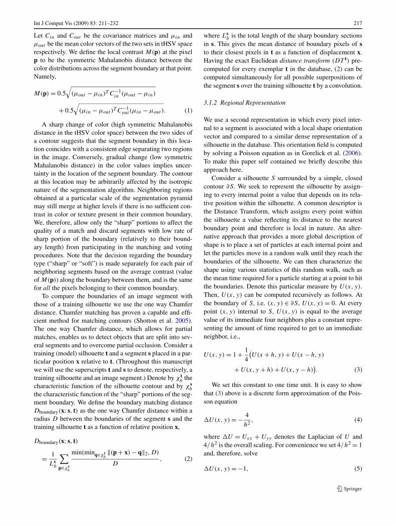
Our detection scheme relies on a matching process in whichimage segments are matched against silhouettes in the data-base. A good match is one in which a segment overlaps fairlyclosely with a portion of a silhouette. To evaluate a matchwe consider two types of representations: boundary and re-gion, denoted by d = “b” and d = “r” respectively. The firstone describes the fit between the boundaries of both the seg-ment and the silhouette, and the second one compares a lo-cal shape descriptor at each of their internal pixels. Belowwe describe in detail the representations and how we judgethe quality of a match.

3.1.1 Boundary Representation

The first representation we use consists of the segmentboundaries. We distinguish between “sharp” (significant)and “soft” (insignificant) sections along the boundaries bymeasuring the local color contrast at every location alongthe boundaries of a segment (see Fig. 4).

For each boundary pixel p consider a disc of radius r

centered at a pixel. Let Vin and Vout denote the sets of discpixels falling inside and outside the segment respectively.

Fig. 4 (a) An input image, (b) its segmentation at one scale of the hi-erarchy, (c) at each boundary point we consider a rectangular patch andmeasure the symmetric Mahalanobis Distance in tHSV space between

the inner and outer parts of the segment, (d) boundary representation,denoted d = “b”, for a particular segment (the green segment in (b))

Int J Comput Vis (2009) 83: 211–232 217

Let Cin and Cout be the covariance matrices and μin andμout be the mean color vectors of the two sets in tHSV spacerespectively. We define the local contrast M(p) at the pixelp to be the symmetric Mahalanobis distance between thecolor distributions across the segment boundary at that point.Namely,

M(p) = 0.5√

(μout − μin)T C−1in (μout − μin)

+ 0.5√

(μin − μout )T C−1out (μin − μout ). (1)

A sharp change of color (high symmetric Mahalanobisdistance in the tHSV color space) between the two sides ofa contour suggests that the segment boundary in this loca-tion coincides with a consistent edge separating two regionsin the image. Conversely, gradual change (low symmetricMahalanobis distance) in the color values implies uncer-tainty in the location of the segment boundary. The contourat this location may be arbitrarily affected by the isotropicnature of the segmentation algorithm. Neighboring regionsobtained at a particular scale of the segmentation pyramidmay still merge at higher levels if there is no sufficient con-trast in color or texture present in their common boundary.We, therefore, allow only the “sharp” portions to affect thequality of a match and discard segments with low rate ofsharp portion of the boundary (relatively to their bound-ary length) from participating in the matching and votingprocedures. Note that the decision regarding the boundarytype (“sharp” or “soft”) is made separately for each pair ofneighboring segments based on the average contrast (valueof M(p)) along the boundary between them, and is the samefor all the pixels belonging to their common boundary.

To compare the boundaries of an image segment withthose of a training silhouette we use the one way Chamferdistance. Chamfer matching has proven a capable and effi-cient method for matching contours (Shotton et al. 2005).The one way Chamfer distance, which allows for partialmatches, enables us to detect objects that are split into sev-eral segments and to overcome partial occlusion. Consider atraining (model) silhouette t and a segment s placed in a par-ticular position x relative to t. (Throughout this manuscriptwe will use the superscripts t and s to denote, respectively, atraining silhouette and an image segment.) Denote by χ t

b thecharacteristic function of the silhouette contour and by χ s

b

the characteristic function of the “sharp” portions of the seg-ment boundary. We define the boundary matching distanceDboundary(x; s, t) as the one way Chamfer distance within aradius D between the boundaries of the segment s and thetraining silhouette t as a function of relative position x,

Dboundary(x; s, t)

= 1

Lsb

∑p∈χ s

b

min(minq∈χ tb‖(p + x) − q‖2,D)

D, (2)

where Lsb is the total length of the sharp boundary sections

in s. This gives the mean distance of boundary pixels of sto their closest pixels in t as a function of displacement x.Having the exact Euclidean distance transform (DT t) pre-computed for every exemplar t in the database, (2) can becomputed simultaneously for all possible superpositions ofthe segment s over the training silhouette t by a convolution.

3.1.2 Regional Representation

We use a second representation in which every pixel inter-nal to a segment is associated with a local shape orientationvector and compared to a similar dense representation of asilhouette in the database. This orientation field is computedby solving a Poisson equation as in Gorelick et al. (2006).To make this paper self contained we briefly describe thisapproach here.

Consider a silhouette S surrounded by a simple, closedcontour ∂S. We seek to represent the silhouette by assign-ing to every internal point a value that depends on its rela-tive position within the silhouette. A common descriptor isthe Distance Transform, which assigns every point withinthe silhouette a value reflecting its distance to the nearestboundary point and therefore is local in nature. An alter-native approach that provides a more global description ofshape is to place a set of particles at each internal point andlet the particles move in a random walk until they reach theboundaries of the silhouette. We can then characterize theshape using various statistics of this random walk, such asthe mean time required for a particle starting at a point to hitthe boundaries. Denote this particular measure by U(x,y).Then, U(x,y) can be computed recursively as follows. Atthe boundary of S, i.e. (x, y) ∈ ∂S, U(x,y) = 0. At everypoint (x, y) internal to S, U(x,y) is equal to the averagevalue of its immediate four neighbors plus a constant repre-senting the amount of time required to get to an immediateneighbor, i.e.,

U(x,y) = 1 + 1

4

(U(x + h,y) + U(x − h,y)

+ U(x,y + h) + U(x,y − h)). (3)

We set this constant to one time unit. It is easy to showthat (3) above is a discrete form approximation of the Pois-son equation

�U(x,y) = − 4

h2, (4)

where �U = Uxx + Uyy denotes the Laplacian of U and4/h2 is the overall scaling. For convenience we set 4/h2 = 1and, therefore, solve

�U(x,y) = −1, (5)

218 Int J Comput Vis (2009) 83: 211–232

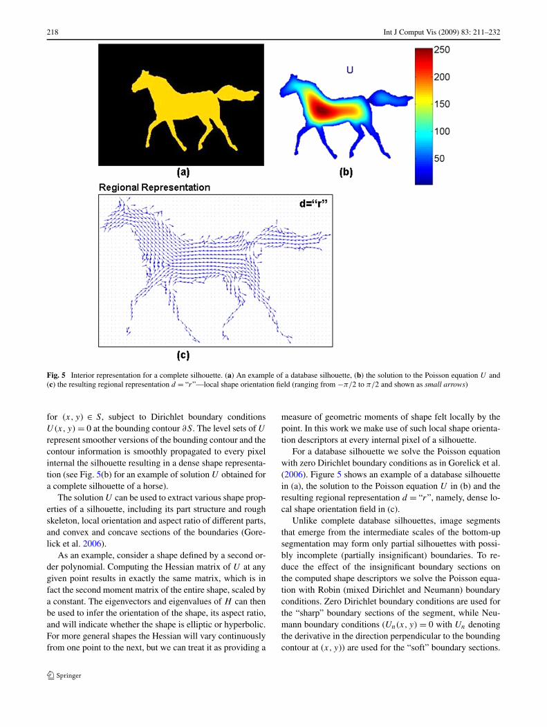
Fig. 5 Interior representation for a complete silhouette. (a) An example of a database silhouette, (b) the solution to the Poisson equation U and(c) the resulting regional representation d = “r”—local shape orientation field (ranging from −π/2 to π/2 and shown as small arrows)

for (x, y) ∈ S, subject to Dirichlet boundary conditionsU(x,y) = 0 at the bounding contour ∂S. The level sets of U

represent smoother versions of the bounding contour and thecontour information is smoothly propagated to every pixelinternal the silhouette resulting in a dense shape representa-tion (see Fig. 5(b) for an example of solution U obtained fora complete silhouette of a horse).

The solution U can be used to extract various shape prop-erties of a silhouette, including its part structure and roughskeleton, local orientation and aspect ratio of different parts,and convex and concave sections of the boundaries (Gore-lick et al. 2006).

As an example, consider a shape defined by a second or-der polynomial. Computing the Hessian matrix of U at anygiven point results in exactly the same matrix, which is infact the second moment matrix of the entire shape, scaled bya constant. The eigenvectors and eigenvalues of H can thenbe used to infer the orientation of the shape, its aspect ratio,and will indicate whether the shape is elliptic or hyperbolic.For more general shapes the Hessian will vary continuouslyfrom one point to the next, but we can treat it as providing a

measure of geometric moments of shape felt locally by thepoint. In this work we make use of such local shape orienta-tion descriptors at every internal pixel of a silhouette.

For a database silhouette we solve the Poisson equationwith zero Dirichlet boundary conditions as in Gorelick et al.(2006). Figure 5 shows an example of a database silhouettein (a), the solution to the Poisson equation U in (b) and theresulting regional representation d = “r”, namely, dense lo-cal shape orientation field in (c).

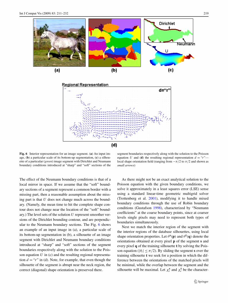
Unlike complete database silhouettes, image segmentsthat emerge from the intermediate scales of the bottom-upsegmentation may form only partial silhouettes with possi-bly incomplete (partially insignificant) boundaries. To re-duce the effect of the insignificant boundary sections onthe computed shape descriptors we solve the Poisson equa-tion with Robin (mixed Dirichlet and Neumann) boundaryconditions. Zero Dirichlet boundary conditions are used forthe “sharp” boundary sections of the segment, while Neu-mann boundary conditions (Un(x, y) = 0 with Un denotingthe derivative in the direction perpendicular to the boundingcontour at (x, y)) are used for the “soft” boundary sections.

Int J Comput Vis (2009) 83: 211–232 219

Fig. 6 Interior representation for an image segment. (a) An input im-age, (b) a particular scale of its bottom-up segmentation, (c) a silhou-ette of a particular (green) image segment with Dirichlet and Neumannboundary conditions introduced at “sharp” and “soft” sections of the

segment boundaries respectively along with the solution to the Poissonequation U and (d) the resulting regional representation d = “r”—local shape orientation field (ranging from −π/2 to π/2 and shown assmall arrows)

The effect of the Neumann boundary conditions is that of alocal mirror in space. If we assume that the “soft” bound-ary sections of a segment represent a common border with amissing part, then a reasonable assumption about the miss-ing part is that U does not change much across the bound-ary. (Namely, the mean time to hit the complete shape con-tour does not change near the location of the “soft” bound-ary.) The level sets of the solution U represent smoother ver-sions of the Dirichlet bounding contour, and are perpendic-ular to the Neumann boundary sections. The Fig. 6 showsan example of an input image in (a), a particular scale ofits bottom-up segmentation in (b), a silhouette of an imagesegment with Dirichlet and Neumann boundary conditionsintroduced at “sharp” and “soft” sections of the segmentboundaries respectively along with the solution to the Pois-son equation U in (c) and the resulting regional representa-tion d = “r” in (d). Note, for example, that even though thesilhouette of the segment is abrupt near the neck region, thecorrect (diagonal) shape orientation is preserved there.

As there might not be an exact analytical solution to thePoisson equation with the given boundary conditions, wesolve it approximately in a least squares error (LSE) senseusing a standard linear-time geometric multigrid solver(Trottenberg et al. 2001), modifying it to handle mixedboundary conditions through the use of Robin boundaryconditions (Gustafson 1998), characterized by “Neumanncoefficients” at the coarse boundary points, since at coarserlevels single pixels may need to represent both types ofboundaries simultaneously.

Next we match the interior region of the segment withthe interior regions of the database silhouettes, using localshape orientation properties. Let θ s(p) and θ t(q) denote theorientations obtained at every pixel p of the segment s andevery pixel q of the training silhouette t by solving the Pois-son equation (|θi | ≤ π/2). By sliding the segment s over thetraining silhouette t we seek for a position in which the dif-ference between the orientations of the matched pixels willbe minimal, while the overlap between the segment and thesilhouette will be maximal. Let χ s

r and χ tr be the character-

220 Int J Comput Vis (2009) 83: 211–232

istic functions of the segment s and the training silhouette trespectively, and let x be a displacement of s relative to t.We define the region matching distance as follows,

Dregion(x; s, t)

=∑p∈χ s

r

d(θ s(p), θ t(p + x)) · χ sr (p) · χ t

r (p + x)

+∑p∈χ s

r

1

2· χ s

r (p) · χ tr (p + x), (6)

where d(θ1, θ2) = 0.5(1 − cos 2(θ1 − θ2)) ranges from zero(for a perfect match) to one (no match) and χ t

r is the com-plement of the characteristic function.

The first term in (6) sums up the difference in orienta-tion of matching pixels in the overlap area, and the sec-ond term counts the number of non-overlapping pixels ofs, assuming that non-overlapping portions match with 1/2,the mean value of d(θ1, θ2). Clearly, Dregion(x; s, t) dependson the size of a segment of interest, but it is compara-ble between the different matches of the same segment.The distance Dregion(x; s, t) can be computed simultane-ously for all possible superpositions of the segment s overthe training silhouette t using the identity cos 2(α − β) =cos(2α) cos(2β) + sin(2α) sin(2β) by a convolution.

Note, that both our boundary and regional representationsare determined by the edges of a segment, but they substan-tially differ in the type of information they describe. Ourboundary representation is local in nature. It marks at everylocation the distance to the nearby edge element. Our re-gional representation, in contrast, provides a more global de-scription of the shape, determined for each location throughaveraging random walk times to all boundary locations.Therefore, for instance, to conclude that a shape is elon-gated in a certain direction we need information about thepresence of two adjacent image contours oriented in roughlythe same direction. This information is not available in theboundary representation of the contours.

3.1.3 Interpretations of a Segment

Consider the collection of training silhouettes in the data-base superimposed one on top the other so that their centersare aligned. We refer to the coordinate system with the ori-gin at their common center location as “an abstract model”or “an abstract coordinate system” of an object class.

Given a particular segment s, it is matched against eachof the training silhouettes in the database resulting in twosets of distance maps, namely {Dboundary(x; s, tk)}Kk=1 and{Dregion(x; s, tk)}Kk=1 (with tk denoting the kth training sil-houette in the database). We apply non-minimal suppressionto each map with a radius proportional to the area of the seg-ment. This results in a collection of preferred locations xi ,

i = 1 . . .Nb +Nr of the segment s relative to the object classabstract model, where Nb and Nr are the total number of se-lected peaks in the two sets of maps accordingly. We referto each such preferred location as an interpretation and de-note it with Ii (or Iij when the segment is denoted by sj ).We further assign a score to each interpretation, reflectingthe quality of the match for that interpretation, which willbe used as a voting weight.

The quality of a boundary based interpretation Ii, i =1 . . .Nb depends on the relative length of the sharp portionof the segment boundary and its Chamfer distance to theboundary of the related exemplar in the database ti , namely,

Qb(Ii) = Lsb

Ls (1 − Dboundary(xi; s, ti )), (7)

where Ls is the total length of the segment boundary in pix-els and Ls

b is the length of the sharp portion of the segmentboundary. We further define the normalized score as

Qb(Ii) = Qb(Ii)∑Nb

l=1 Qb(Il). (8)

The quality of a region based interpretation Ii, i = Nb +1 . . .Nb + Nr depends on the similarity in the orientation ofthe matched pixels and the size of the explained portion ofthe segment, that is

Qr(Ii) = 1

As

∑p∈χ s

r

(1 − d(θ s(p), θ ti (p + xi ))

)

× χ sr (p) · χ ti

r (p + xi ), (9)

where As denotes the area of the segment in pixels. Again,we define the normalized score as

Qr (Ii) = Qr(Ii)∑Nb+Nr

l=Nb+1 Qr(Il). (10)

Note, that the boundary and region matching distances in(2) and (6) are used to find the preferred interpretations (lo-cal minima in the distance map) among the interpretationsoriginating from the same training silhouette, whereas thequality scores of boundary and region interpretations in (8)and (10) are used to weight the interpretation relatively tointerpretations originating from other training silhouettes.

3.2 Detection

In this and the next sections we provide a probabilistic for-mulation for the detection and top-down segmentation.

Our detection scheme follows the principles proposedin Leibe et al. (2008) while being reformulated to handlesegments of varying shapes and sizes and to incorporatedense local shape properties into the voting process.

Int J Comput Vis (2009) 83: 211–232 221

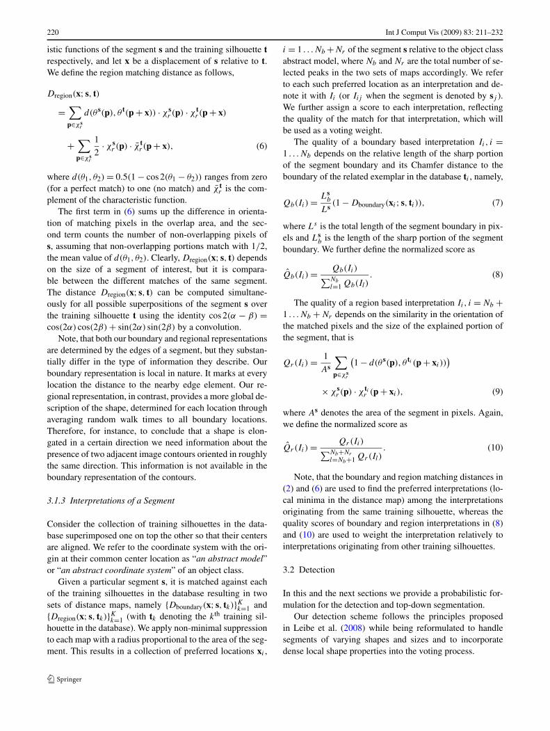
Fig. 7 The graphical model ofthe detection stage

Given a test image Img, consider a particular scale of thesegmentation pyramid. Let sj = (cj , θj , lj ,bj ) denote thecolor and orientation information associated with pixels ofa segment j observed at location lj along with its bound-ary information. Denote by s the random variable represent-ing the index of an image segment, s = sj , j ∈ {1, . . . , n}.Let d be the random variable corresponding to the consid-ered shape representation, (d ∈ {b, r} standing for boundaryor region representation). Let x and o denote the randomvariables corresponding to the location in the image of theobject of a certain class accordingly. See Fig. 7 for a depic-tion of the graphical model and a list of random variablesalong with their domains. (Note that the identity of the testimage Img is observed, and the computations derived fromthe graphical model and described hereafter are all condi-tioned on it. For clarity we omit the conditioning throughoutthis section.) The joint probability of observing an object ofthe class o at location x given the segment s and the chosenrepresentation d is defined by

p(o, x|s, d) = p(o|s, d)p(x|s, o, d)

= p(o|s)p(x|s, o, d) (11)

where we choose the first term, p(o|s, d), to reflect ourconfidence that the segment s belongs to the class o basedsolely on its appearance (e.g., its color), and so it is inde-pendent of the chosen shape representation d . The secondterm, p(x|s, o, d), is a probabilistic Hough vote for objectposition x based on the shape information of the segment.

For the term, p(o|s), we learn a discrete probability dis-tribution over the first two coordinates of a tHSV colorspace. Using segmented training data we construct two100 × 100 bins color histograms providing the probabili-ties to observe a specific color c at pixels belonging to classand non-class respectively, namely, p(c|o) and p(c|o). As-suming a uniform prior for p(o) and p(o), the probability

to observe an object class o given the color c is p(o|c) =p(c|o)/(p(c|o)+p(c|o)). Finally, for the confidence p(o|s)that a segment s belongs to a class based on its color we thenuse the mean of these probabilities over the pixels of s.

For the second term, p(x|s = sj , o, d) in (11), we use theset of interpretations {Ii |d, o, s = sj } obtained by match-ing the segment sj to the silhouettes in the database usingthe shape representation d as described in Sects. 3.1.1 and3.1.2. Given that s is a part of an object of class o, let theterm p(I = Ii |s = sj , o, d) reflect our confidence in inter-preting the segment s by I using the shape representation d .This confidence is set to be the normalized quality of thematch between the segment and the related training silhou-ette, Qd(I ) (see (8), (10)). Each interpretation then votesfor possible center locations x of the object with probabilityp(x|s, o, I, d) which is independent of the representation d

chosen. We model this probability by a Gaussian distribu-tion whose mean is determined by the relative location ofthe interpretation in the database silhouette and with con-stant variance σ (we used σ = 8). By marginalizing (11)over the set of interpretations we obtain

p(o, x|s, d) = p(o|s)p(x|s, o, d)

= p(o|s)∑I

p(x, I |s, o, d)

= p(o|s)∑I

p(x|s, o, I, d)p(I |s, o, d). (12)

The single-segment votes are marginalized to obtain theprobability of a hypothesis h = (o, x),

p(o, x) =∑

d∈{b,r}p(o, x, d)

=∑

d∈{b,r}p(d)p(o, x|d)

222 Int J Comput Vis (2009) 83: 211–232

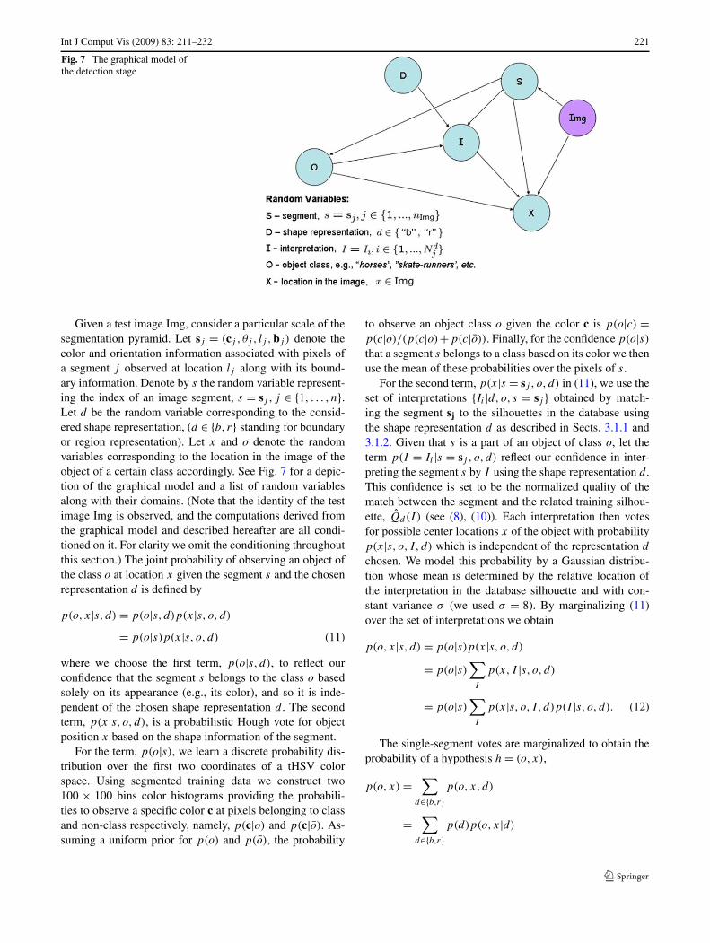
Fig. 8 The graphical model ofthe back-projection stage

=∑

d∈{b,r}p(d)

∑s

p(o, x, s|d)

=∑

d∈{b,r}p(d)

∑s

p(o, x|s, d)p(s|d) (13)

with a uniform prior p(d) and probability p(s|d) set to beproportional to the size of the segment s relatively to othersegments of the same scale in the segmentation pyramid.The probabilities p(o, x) are computed simultaneously forall x resulting in a “voting map” (see Fig. 10, second row,column (a)). See Table 1 for a pseudocode of the detectionalgorithm.

3.3 Top-Down Segmentation

Given a detection hypothesis h = (x, o) obtained with thebottom-up detection process, our next goal is to segment theobject from its background.

One way to do this is to simply select all the segmentsthat voted with significant probability for this hypothesisalong with their interpretations. For each such interpretationIi , it is possible to only consider the part of the segment sj

that is matched to the inside of the related database silhou-ette. Combining the information from all the interpretationsof the segment would result in a probability map determin-ing which pixels of the segment belongs to the foregroundor the background. This, back-projection approach is sim-ilar to the top-down segmentation proposed in Leibe et al.(2008). However, it does not distinguish between correctand erroneous votes of different segments that accidentallymatched to (or were interpreted by) the same semantic partof the model (e.g., the correct votes of the green segment vs.the erroneous votes of the pink segment shown in Fig. 3).Therefore, such a naive back-projection approach may give

rise to a “ghosting effect,” whereby the segmentation resultsinclude, e.g., “extra” back or limbs, see also Fig. 10, bot-tom row, column (b). To address this problem we introducea competitive coverage approach, in which we let the seg-ments compete for those parts.

We begin by formulating the back-projection approach.

3.3.1 Segmentation by Back-Projection

Our aim in this part is to identify the pixels that votedstrongly to the object in its considered location. Given anobject hypothesis h = (o, x) and segment s = sj , denote byum the event that a segment pixel pm ∈ sj belongs to theforeground object. The relevant graphical model is shown inFig. 8. The probability of this event is given by

p(um|o, x, s) =∑

d∈{b,r}p(um,d|o, x, s)

=∑

d∈{b,r}p(d|o, x, s)p(um|o, x, s, d) (14)

=∑

d∈{b,r}p(d)

p(um,o, x|s, d)

p(o, x|s, d). (15)

The first transition is a simple marginalization over the pos-sible shape representations. Assuming the shape representa-tion d is independent of the class object o, position x andsegment s, the last transition follows from the Bayes’ rule.

Consider the numerator p(um,o, x|s, d) in (15). This isthe joint probability for the hypothesis h = (o, x) and for thesegment pixel pm to belong to the foreground of the object,given the segment s = sj and using the shape representa-tion d . To compute it, we marginalize over those interpreta-tions of s in which pm participated as foreground pixel (i.e.,was matched to the inside of the related database silhouette)to obtain:

Int J Comput Vis (2009) 83: 211–232 223

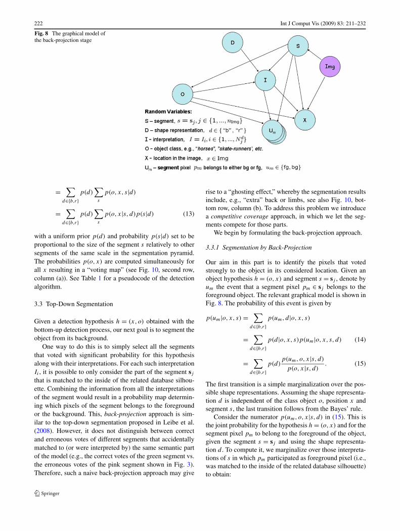
Fig. 9 The graphical model ofthe competitive-coverage stage

p(um,o, x|s, d)

= p(o|s, d)p(um,x|s, o, d) (16)

= p(o|s)∑I

p(um,x, I |s, o, d) (17)

= p(o|s)∑I

p(x|s, o, I, um,d)p(um|s, o, I, d)

× p(I |s, o, d) (18)

= p(o|s)∑I

p(x|s, o, I )p(um|s, o, I )p(I |s, o, d). (19)

The term p(o|s, d) in (16) depends solely on the appear-

ance of sj and is independent of the shape representation d .

The transition to (17) is due to marginalization of the inter-

pretations I of the segment s. The term p(x|s, o, I, um,d)

in (18) is the probabilistic Hough vote of the interpretation

I for an object location. It is dependent on the location of

the segment l and the interpretation I , but is independent of

a particular pixel um and the representation d chosen. The

term p(um|s, o, I, d) in (18) is one if pm is explained by

the interpretation I (i.e., matches to the inside of the related

database silhouette) and vanishes otherwise. It is, therefore,

independent of the shape representation d as well. Finally,

the last term p(I |s, o, d) in (19) is the normalized matching

quality, Qd(I ), computed as in (8) and (10).

The collection of the probabilities p(um|o, x, s = sj ) in

(14), computed ∀pm ∈ sj forms the “back-projection” map

of the segment. Figure 10, second row, column (b) shows an

example of back-projection map simultaneously for all the

segments of a particular segmentation scale.

3.3.2 Segmentation by Competitive Coverage

To incorporate competition in the process we distinguish be-tween the segment pixels pm, which may or may not belongto the foreground object o in the image, and the pixels in anabstract model of an object (defined in Sect. 3.1.3), whichmay or may not be covered (explained) by the image pix-els. We denote by k = (xk, yk) the coordinates of a pixel qk

in an abstract model of an object and seek the most proba-ble cover of the model pixel qk by an image segment. For agiven hypothesis h = (o, x), denote by vk the event that hy-pothesis h covers the pixel qk . The graphical model of thisprocess is illustrated in Fig. 9. The probability that (amongall the segments) a segment s = sj covers model pixel qk

can be written as

p(s|o, x, vk) =∑

d∈{b,r}p(d|o, x, vk)p(s|o, x, vk, d) (20)

=∑

d∈{b,r}p(d)

p(vk, o, x|s, d)p(s|d)

p(vk, o, x|d), (21)

where the first transition is a marginalization over the shaperepresentation d and the second transition follows Bayes’rule. Here again, we assume the shape representation d isindependent of the class object o, position x and pixel vk .

The term p(vk, o, x|s, d) in the numerator of (21) reflectsthe joint probability of the hypothesis h = (o, x) and theevent that the model pixel qk is covered by the segment s

using the shape representation d . Again, we sum only overthose interpretations of the segment s that explain the modelpixel qk , (i.e., have the pixel qk of the related database sil-houette in the overlap area),

224 Int J Comput Vis (2009) 83: 211–232

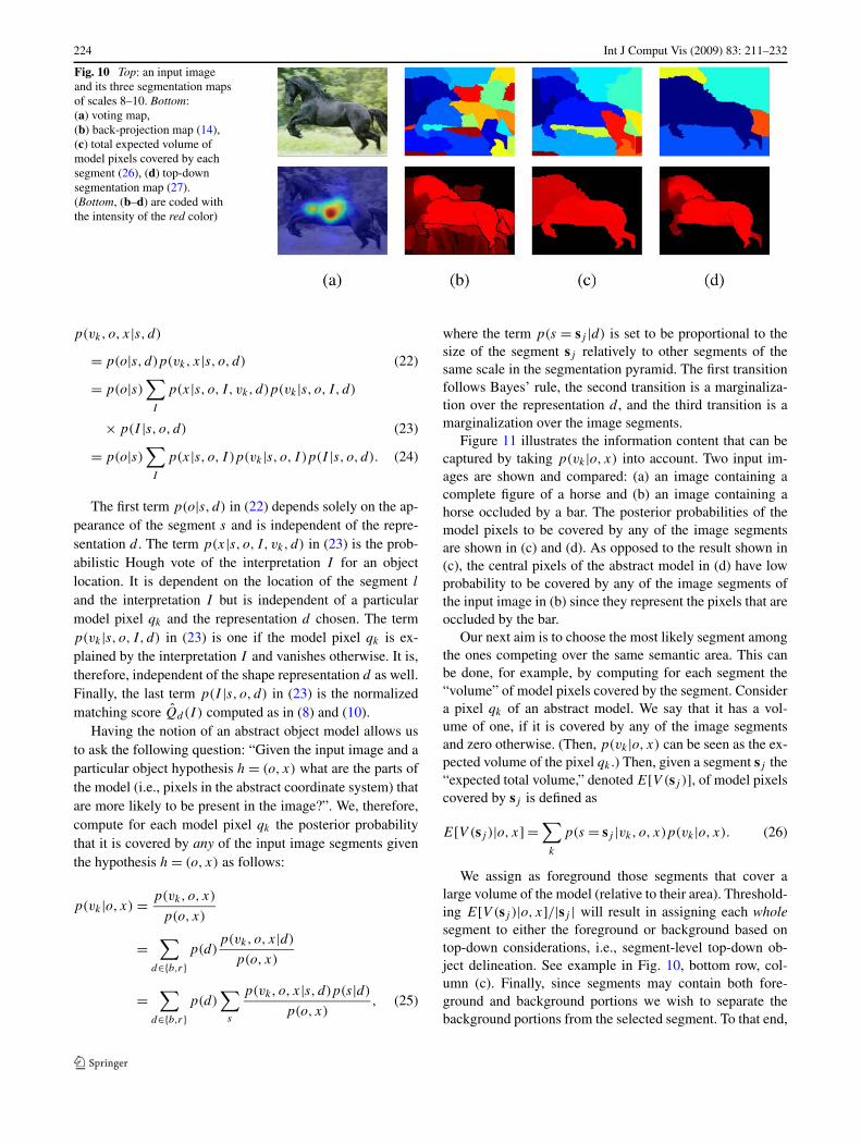
Fig. 10 Top: an input imageand its three segmentation mapsof scales 8–10. Bottom:(a) voting map,(b) back-projection map (14),(c) total expected volume ofmodel pixels covered by eachsegment (26), (d) top-downsegmentation map (27).(Bottom, (b–d) are coded withthe intensity of the red color)

p(vk, o, x|s, d)

= p(o|s, d)p(vk, x|s, o, d) (22)

= p(o|s)∑I

p(x|s, o, I, vk, d)p(vk|s, o, I, d)

× p(I |s, o, d) (23)

= p(o|s)∑I

p(x|s, o, I )p(vk|s, o, I )p(I |s, o, d). (24)

The first term p(o|s, d) in (22) depends solely on the ap-pearance of the segment s and is independent of the repre-sentation d . The term p(x|s, o, I, vk, d) in (23) is the prob-abilistic Hough vote of the interpretation I for an objectlocation. It is dependent on the location of the segment l

and the interpretation I but is independent of a particularmodel pixel qk and the representation d chosen. The termp(vk|s, o, I, d) in (23) is one if the model pixel qk is ex-plained by the interpretation I and vanishes otherwise. It is,therefore, independent of the shape representation d as well.Finally, the last term p(I |s, o, d) in (23) is the normalizedmatching score Qd(I ) computed as in (8) and (10).

Having the notion of an abstract object model allows usto ask the following question: “Given the input image and aparticular object hypothesis h = (o, x) what are the parts ofthe model (i.e., pixels in the abstract coordinate system) thatare more likely to be present in the image?”. We, therefore,compute for each model pixel qk the posterior probabilitythat it is covered by any of the input image segments giventhe hypothesis h = (o, x) as follows:

p(vk|o, x) = p(vk, o, x)

p(o, x)

=∑

d∈{b,r}p(d)

p(vk, o, x|d)

p(o, x)

=∑

d∈{b,r}p(d)

∑s

p(vk, o, x|s, d)p(s|d)

p(o, x), (25)

where the term p(s = sj |d) is set to be proportional to thesize of the segment sj relatively to other segments of thesame scale in the segmentation pyramid. The first transitionfollows Bayes’ rule, the second transition is a marginaliza-tion over the representation d , and the third transition is amarginalization over the image segments.

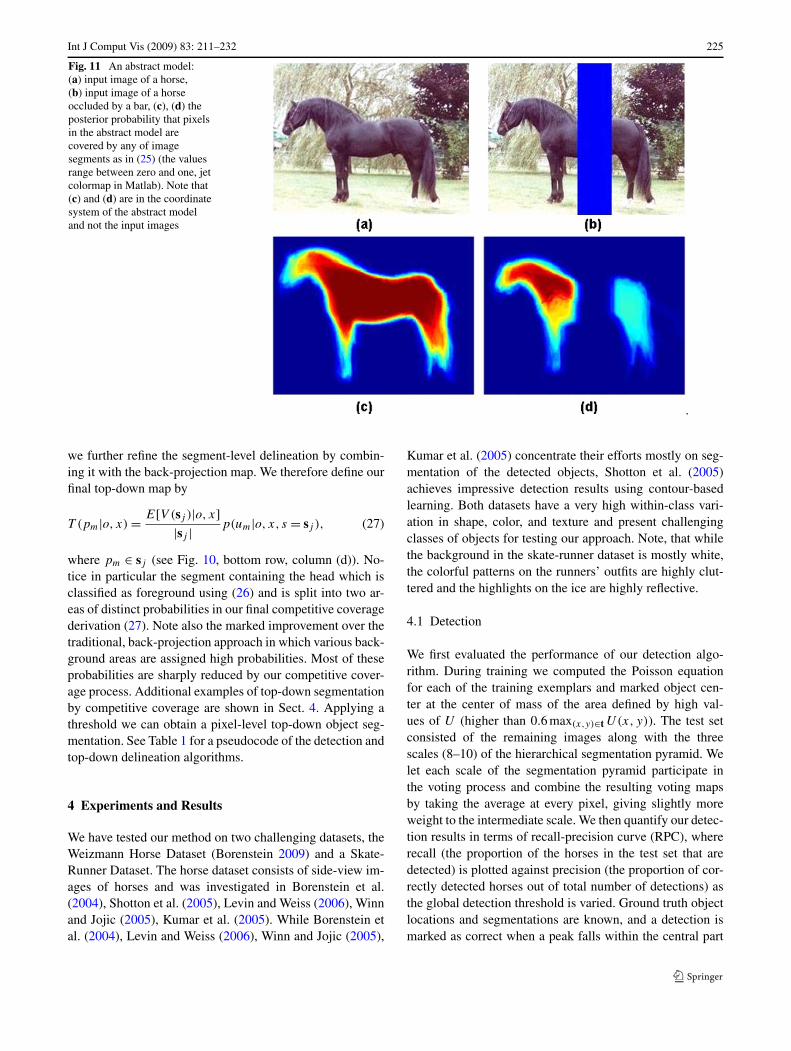
Figure 11 illustrates the information content that can becaptured by taking p(vk|o, x) into account. Two input im-ages are shown and compared: (a) an image containing acomplete figure of a horse and (b) an image containing ahorse occluded by a bar. The posterior probabilities of themodel pixels to be covered by any of the image segmentsare shown in (c) and (d). As opposed to the result shown in(c), the central pixels of the abstract model in (d) have lowprobability to be covered by any of the image segments ofthe input image in (b) since they represent the pixels that areoccluded by the bar.

Our next aim is to choose the most likely segment amongthe ones competing over the same semantic area. This canbe done, for example, by computing for each segment the“volume” of model pixels covered by the segment. Considera pixel qk of an abstract model. We say that it has a vol-ume of one, if it is covered by any of the image segmentsand zero otherwise. (Then, p(vk|o, x) can be seen as the ex-pected volume of the pixel qk .) Then, given a segment sj the“expected total volume,” denoted E[V (sj )], of model pixelscovered by sj is defined as

E[V (sj )|o, x] =∑

k

p(s = sj |vk, o, x)p(vk|o, x). (26)

We assign as foreground those segments that cover alarge volume of the model (relative to their area). Threshold-ing E[V (sj )|o, x]/|sj | will result in assigning each wholesegment to either the foreground or background based ontop-down considerations, i.e., segment-level top-down ob-ject delineation. See example in Fig. 10, bottom row, col-umn (c). Finally, since segments may contain both fore-ground and background portions we wish to separate thebackground portions from the selected segment. To that end,

Int J Comput Vis (2009) 83: 211–232 225

Fig. 11 An abstract model:(a) input image of a horse,(b) input image of a horseoccluded by a bar, (c), (d) theposterior probability that pixelsin the abstract model arecovered by any of imagesegments as in (25) (the valuesrange between zero and one, jetcolormap in Matlab). Note that(c) and (d) are in the coordinatesystem of the abstract modeland not the input images

.

we further refine the segment-level delineation by combin-ing it with the back-projection map. We therefore define ourfinal top-down map by

T (pm|o, x) = E[V (sj )|o, x]|sj | p(um|o, x, s = sj ), (27)

where pm ∈ sj (see Fig. 10, bottom row, column (d)). No-tice in particular the segment containing the head which isclassified as foreground using (26) and is split into two ar-eas of distinct probabilities in our final competitive coveragederivation (27). Note also the marked improvement over thetraditional, back-projection approach in which various back-ground areas are assigned high probabilities. Most of theseprobabilities are sharply reduced by our competitive cover-age process. Additional examples of top-down segmentationby competitive coverage are shown in Sect. 4. Applying athreshold we can obtain a pixel-level top-down object seg-mentation. See Table 1 for a pseudocode of the detection andtop-down delineation algorithms.

4 Experiments and Results

We have tested our method on two challenging datasets, theWeizmann Horse Dataset (Borenstein 2009) and a Skate-Runner Dataset. The horse dataset consists of side-view im-ages of horses and was investigated in Borenstein et al.(2004), Shotton et al. (2005), Levin and Weiss (2006), Winnand Jojic (2005), Kumar et al. (2005). While Borenstein etal. (2004), Levin and Weiss (2006), Winn and Jojic (2005),

Kumar et al. (2005) concentrate their efforts mostly on seg-mentation of the detected objects, Shotton et al. (2005)achieves impressive detection results using contour-basedlearning. Both datasets have a very high within-class vari-ation in shape, color, and texture and present challengingclasses of objects for testing our approach. Note, that whilethe background in the skate-runner dataset is mostly white,the colorful patterns on the runners’ outfits are highly clut-tered and the highlights on the ice are highly reflective.

4.1 Detection

We first evaluated the performance of our detection algo-rithm. During training we computed the Poisson equationfor each of the training exemplars and marked object cen-ter at the center of mass of the area defined by high val-ues of U (higher than 0.6 max(x,y)∈t U(x,y)). The test setconsisted of the remaining images along with the threescales (8–10) of the hierarchical segmentation pyramid. Welet each scale of the segmentation pyramid participate inthe voting process and combine the resulting voting mapsby taking the average at every pixel, giving slightly moreweight to the intermediate scale. We then quantify our detec-tion results in terms of recall-precision curve (RPC), whererecall (the proportion of the horses in the test set that aredetected) is plotted against precision (the proportion of cor-rectly detected horses out of total number of detections) asthe global detection threshold is varied. Ground truth objectlocations and segmentations are known, and a detection ismarked as correct when a peak falls within the central part

226 Int J Comput Vis (2009) 83: 211–232

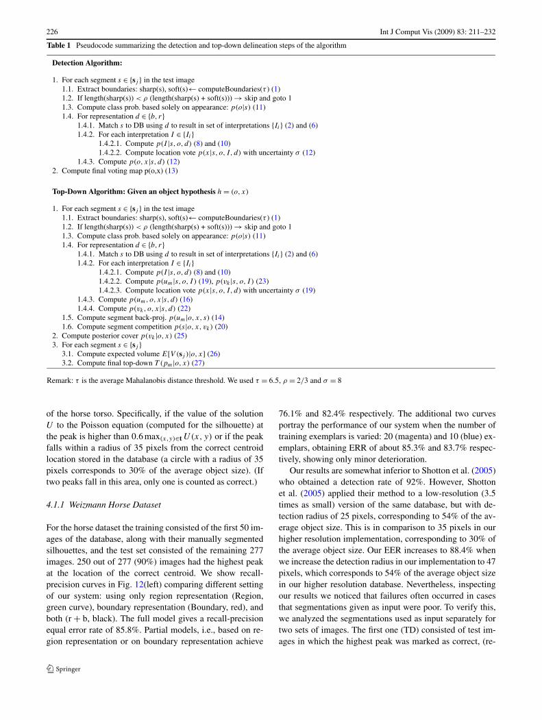
Table 1 Pseudocode summarizing the detection and top-down delineation steps of the algorithm

Detection Algorithm:

1. For each segment s ∈ {sj } in the test image1.1. Extract boundaries: sharp(s), soft(s)← computeBoundaries(τ ) (1)1.2. If length(sharp(s)) < ρ (length(sharp(s) + soft(s))) → skip and goto 11.3. Compute class prob. based solely on appearance: p(o|s) (11)1.4. For representation d ∈ {b, r}

1.4.1. Match s to DB using d to result in set of interpretations {Ii} (2) and (6)1.4.2. For each interpretation I ∈ {Ii}

1.4.2.1. Compute p(I |s, o, d) (8) and (10)1.4.2.2. Compute location vote p(x|s, o, I, d) with uncertainty σ (12)

1.4.3. Compute p(o, x|s, d) (12)2. Compute final voting map p(o,x) (13)

Top-Down Algorithm: Given an object hypothesis h = (o, x)

1. For each segment s ∈ {sj } in the test image1.1. Extract boundaries: sharp(s), soft(s)← computeBoundaries(τ ) (1)1.2. If length(sharp(s)) < ρ (length(sharp(s) + soft(s))) → skip and goto 11.3. Compute class prob. based solely on appearance: p(o|s) (11)1.4. For representation d ∈ {b, r}

1.4.1. Match s to DB using d to result in set of interpretations {Ii} (2) and (6)1.4.2. For each interpretation I ∈ {Ii}

1.4.2.1. Compute p(I |s, o, d) (8) and (10)1.4.2.2. Compute p(um|s, o, I ) (19), p(vk |s, o, I ) (23)1.4.2.3. Compute location vote p(x|s, o, I, d) with uncertainty σ (19)

1.4.3. Compute p(um,o, x|s, d) (16)1.4.4. Compute p(vk, o, x|s, d) (22)

1.5. Compute segment back-proj. p(um|o, x, s) (14)1.6. Compute segment competition p(s|o, x, vk) (20)

2. Compute posterior cover p(vk |o, x) (25)3. For each segment s ∈ {sj }

3.1. Compute expected volume E[V (sj )|o, x] (26)3.2. Compute final top-down T (pm|o, x) (27)

Remark: τ is the average Mahalanobis distance threshold. We used τ = 6.5, ρ = 2/3 and σ = 8

of the horse torso. Specifically, if the value of the solutionU to the Poisson equation (computed for the silhouette) atthe peak is higher than 0.6 max(x,y)∈t U(x,y) or if the peakfalls within a radius of 35 pixels from the correct centroidlocation stored in the database (a circle with a radius of 35pixels corresponds to 30% of the average object size). (Iftwo peaks fall in this area, only one is counted as correct.)

4.1.1 Weizmann Horse Dataset

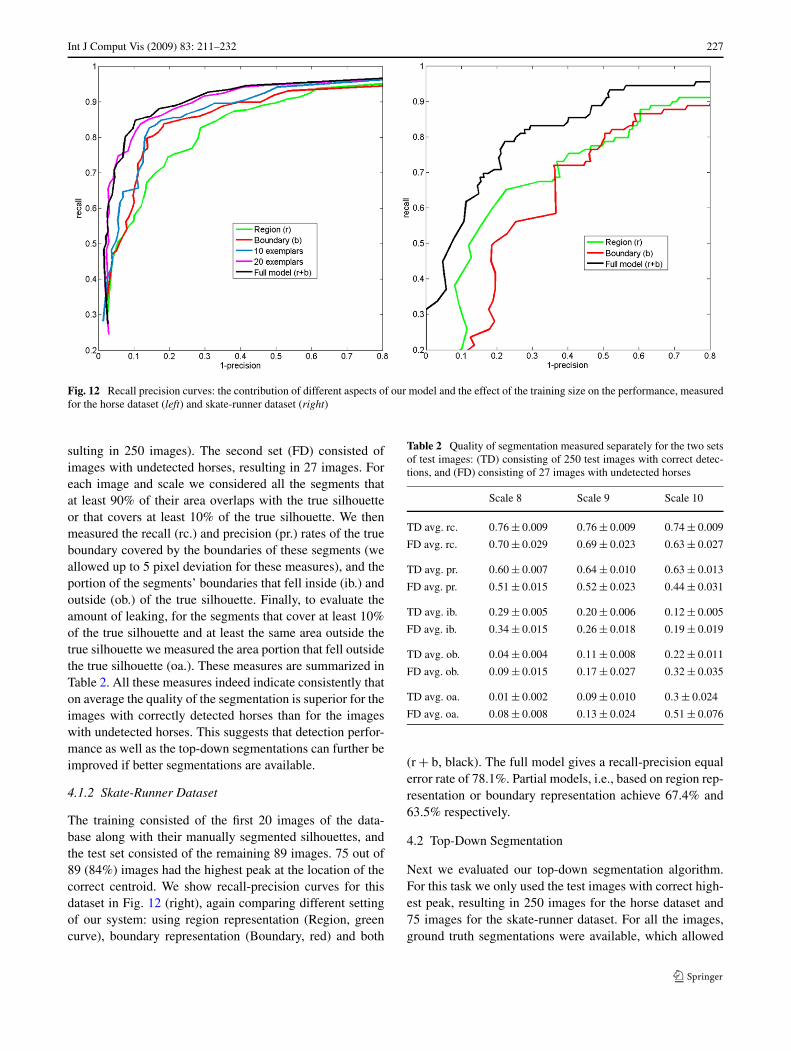
For the horse dataset the training consisted of the first 50 im-ages of the database, along with their manually segmentedsilhouettes, and the test set consisted of the remaining 277images. 250 out of 277 (90%) images had the highest peakat the location of the correct centroid. We show recall-precision curves in Fig. 12(left) comparing different settingof our system: using only region representation (Region,green curve), boundary representation (Boundary, red), andboth (r + b, black). The full model gives a recall-precisionequal error rate of 85.8%. Partial models, i.e., based on re-gion representation or on boundary representation achieve

76.1% and 82.4% respectively. The additional two curvesportray the performance of our system when the number oftraining exemplars is varied: 20 (magenta) and 10 (blue) ex-emplars, obtaining ERR of about 85.3% and 83.7% respec-tively, showing only minor deterioration.

Our results are somewhat inferior to Shotton et al. (2005)who obtained a detection rate of 92%. However, Shottonet al. (2005) applied their method to a low-resolution (3.5times as small) version of the same database, but with de-tection radius of 25 pixels, corresponding to 54% of the av-erage object size. This is in comparison to 35 pixels in ourhigher resolution implementation, corresponding to 30% ofthe average object size. Our EER increases to 88.4% whenwe increase the detection radius in our implementation to 47pixels, which corresponds to 54% of the average object sizein our higher resolution database. Nevertheless, inspectingour results we noticed that failures often occurred in casesthat segmentations given as input were poor. To verify this,we analyzed the segmentations used as input separately fortwo sets of images. The first one (TD) consisted of test im-ages in which the highest peak was marked as correct, (re-

Int J Comput Vis (2009) 83: 211–232 227

Fig. 12 Recall precision curves: the contribution of different aspects of our model and the effect of the training size on the performance, measuredfor the horse dataset (left) and skate-runner dataset (right)

sulting in 250 images). The second set (FD) consisted ofimages with undetected horses, resulting in 27 images. Foreach image and scale we considered all the segments thatat least 90% of their area overlaps with the true silhouetteor that covers at least 10% of the true silhouette. We thenmeasured the recall (rc.) and precision (pr.) rates of the trueboundary covered by the boundaries of these segments (weallowed up to 5 pixel deviation for these measures), and theportion of the segments’ boundaries that fell inside (ib.) andoutside (ob.) of the true silhouette. Finally, to evaluate theamount of leaking, for the segments that cover at least 10%of the true silhouette and at least the same area outside thetrue silhouette we measured the area portion that fell outsidethe true silhouette (oa.). These measures are summarized inTable 2. All these measures indeed indicate consistently thaton average the quality of the segmentation is superior for theimages with correctly detected horses than for the imageswith undetected horses. This suggests that detection perfor-mance as well as the top-down segmentations can further beimproved if better segmentations are available.

4.1.2 Skate-Runner Dataset

The training consisted of the first 20 images of the data-base along with their manually segmented silhouettes, andthe test set consisted of the remaining 89 images. 75 out of89 (84%) images had the highest peak at the location of thecorrect centroid. We show recall-precision curves for thisdataset in Fig. 12 (right), again comparing different settingof our system: using region representation (Region, greencurve), boundary representation (Boundary, red) and both

Table 2 Quality of segmentation measured separately for the two setsof test images: (TD) consisting of 250 test images with correct detec-tions, and (FD) consisting of 27 images with undetected horses

Scale 8 Scale 9 Scale 10

TD avg. rc. 0.76 ± 0.009 0.76 ± 0.009 0.74 ± 0.009

FD avg. rc. 0.70 ± 0.029 0.69 ± 0.023 0.63 ± 0.027

TD avg. pr. 0.60 ± 0.007 0.64 ± 0.010 0.63 ± 0.013

FD avg. pr. 0.51 ± 0.015 0.52 ± 0.023 0.44 ± 0.031

TD avg. ib. 0.29 ± 0.005 0.20 ± 0.006 0.12 ± 0.005

FD avg. ib. 0.34 ± 0.015 0.26 ± 0.018 0.19 ± 0.019

TD avg. ob. 0.04 ± 0.004 0.11 ± 0.008 0.22 ± 0.011

FD avg. ob. 0.09 ± 0.015 0.17 ± 0.027 0.32 ± 0.035

TD avg. oa. 0.01 ± 0.002 0.09 ± 0.010 0.3 ± 0.024

FD avg. oa. 0.08 ± 0.008 0.13 ± 0.024 0.51 ± 0.076

(r + b, black). The full model gives a recall-precision equalerror rate of 78.1%. Partial models, i.e., based on region rep-resentation or boundary representation achieve 67.4% and63.5% respectively.

4.2 Top-Down Segmentation

Next we evaluated our top-down segmentation algorithm.For this task we only used the test images with correct high-est peak, resulting in 250 images for the horse dataset and75 images for the skate-runner dataset. For all the images,ground truth segmentations were available, which allowed

228 Int J Comput Vis (2009) 83: 211–232

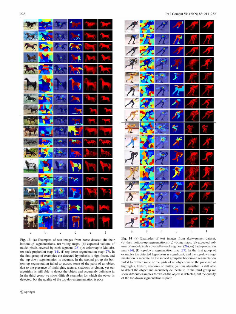
Fig. 13 (a) Examples of test images from horse dataset, (b) theirbottom-up segmentations, (c) voting maps, (d) expected volume ofmodel pixels covered by each segment (26) (jet colormap in Matlab),(e) back-projection map (14), (f) top-down segmentation map (27). Inthe first group of examples the detected hypothesis is significant, andthe top-down segmentation is accurate. In the second group the bot-tom-up segmentation failed to extract some of the parts of an objectdue to the presence of highlights, texture, shadows or clutter, yet ouralgorithm is still able to detect the object and accurately delineate it.In the third group we show difficult examples for which the object isdetected, but the quality of the top-down segmentation is poor

Fig. 14 (a) Examples of test images from skate-runner dataset,(b) their bottom-up segmentations, (c) voting maps, (d) expected vol-ume of model pixels covered by each segment (26), (e) back-projectionmap (14), (f) top-down segmentation map (27). In the first group ofexamples the detected hypothesis is significant, and the top-down seg-mentation is accurate. In the second group the bottom-up segmentationfailed to extract some of the parts of an object due to the presence ofhighlights, texture, shadows or clutter, yet our algorithm is still ableto detect the object and accurately delineate it. In the third group weshow difficult examples for which the object is detected, but the qualityof the top-down segmentation is poor

Int J Comput Vis (2009) 83: 211–232 229

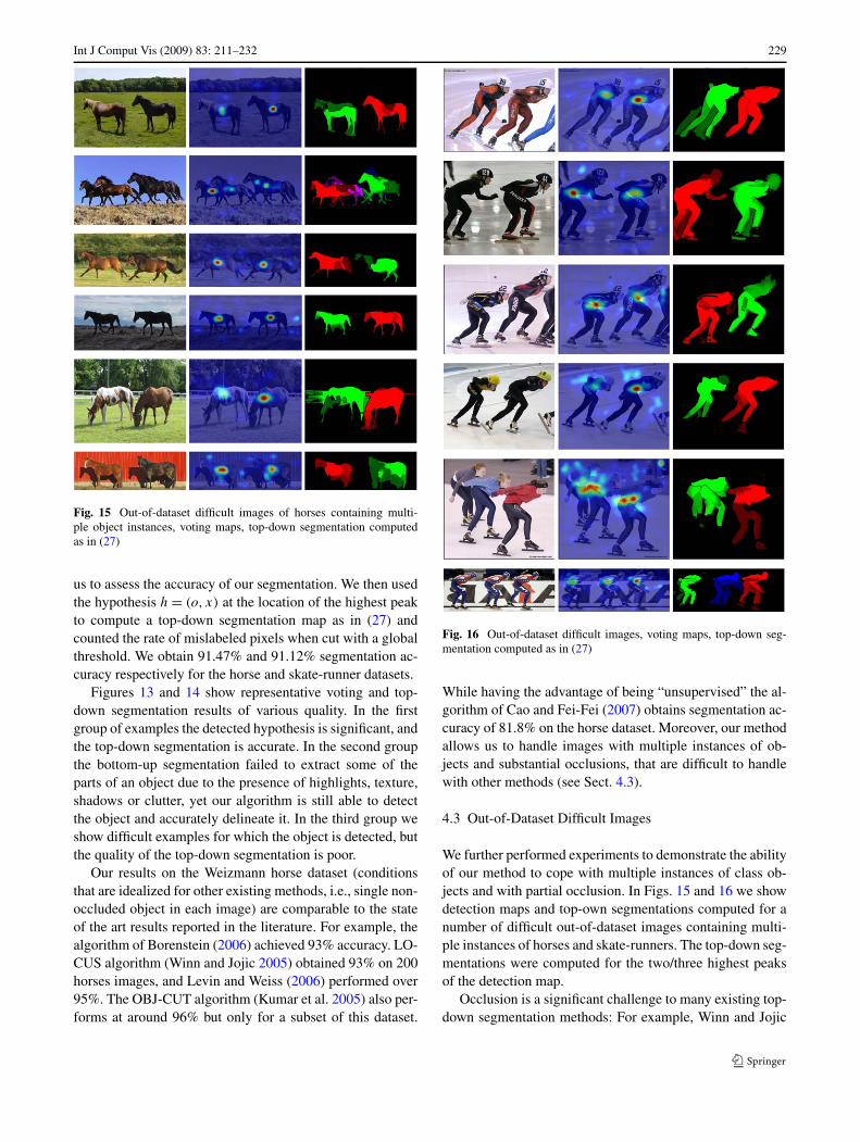
Fig. 15 Out-of-dataset difficult images of horses containing multi-ple object instances, voting maps, top-down segmentation computedas in (27)

us to assess the accuracy of our segmentation. We then usedthe hypothesis h = (o, x) at the location of the highest peakto compute a top-down segmentation map as in (27) andcounted the rate of mislabeled pixels when cut with a globalthreshold. We obtain 91.47% and 91.12% segmentation ac-curacy respectively for the horse and skate-runner datasets.

Figures 13 and 14 show representative voting and top-down segmentation results of various quality. In the firstgroup of examples the detected hypothesis is significant, andthe top-down segmentation is accurate. In the second groupthe bottom-up segmentation failed to extract some of theparts of an object due to the presence of highlights, texture,shadows or clutter, yet our algorithm is still able to detectthe object and accurately delineate it. In the third group weshow difficult examples for which the object is detected, butthe quality of the top-down segmentation is poor.

Our results on the Weizmann horse dataset (conditionsthat are idealized for other existing methods, i.e., single non-occluded object in each image) are comparable to the stateof the art results reported in the literature. For example, thealgorithm of Borenstein (2006) achieved 93% accuracy. LO-CUS algorithm (Winn and Jojic 2005) obtained 93% on 200horses images, and Levin and Weiss (2006) performed over95%. The OBJ-CUT algorithm (Kumar et al. 2005) also per-forms at around 96% but only for a subset of this dataset.

Fig. 16 Out-of-dataset difficult images, voting maps, top-down seg-mentation computed as in (27)

While having the advantage of being “unsupervised” the al-gorithm of Cao and Fei-Fei (2007) obtains segmentation ac-curacy of 81.8% on the horse dataset. Moreover, our methodallows us to handle images with multiple instances of ob-jects and substantial occlusions, that are difficult to handlewith other methods (see Sect. 4.3).

4.3 Out-of-Dataset Difficult Images

We further performed experiments to demonstrate the abilityof our method to cope with multiple instances of class ob-jects and with partial occlusion. In Figs. 15 and 16 we showdetection maps and top-own segmentations computed for anumber of difficult out-of-dataset images containing multi-ple instances of horses and skate-runners. The top-down seg-mentations were computed for the two/three highest peaksof the detection map.

Occlusion is a significant challenge to many existing top-down segmentation methods: For example, Winn and Jojic

230 Int J Comput Vis (2009) 83: 211–232

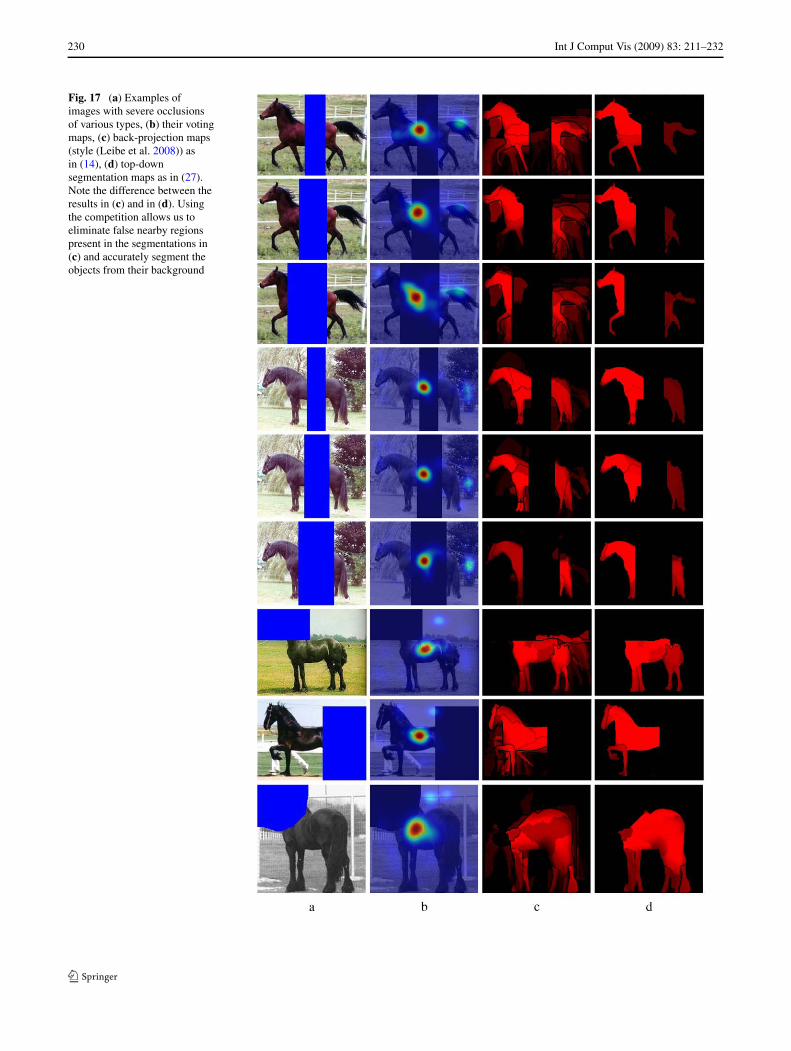
Fig. 17 (a) Examples ofimages with severe occlusionsof various types, (b) their votingmaps, (c) back-projection maps(style (Leibe et al. 2008)) asin (14), (d) top-downsegmentation maps as in (27).Note the difference between theresults in (c) and in (d). Usingthe competition allows us toeliminate false nearby regionspresent in the segmentations in(c) and accurately segment theobjects from their background

Int J Comput Vis (2009) 83: 211–232 231

Fig. 18 (a) Examples of images containing two instances of horsesand showing severe occlusions of various type, (b) their voting maps,(c) back-projection maps (style (Leibe et al. 2008)) as in (14), (d) top-down segmentation maps as in (27). As can be seen in column (d) our

competitive coverage process allows us to correctly assign image pix-els to either red or green object instances as well as sharply delineatetheir boundaries

(2005) assumes smooth deformation field of the object classmask. Levin and Weiss (2006) assumes detection resultingin a bounding box as a preprocessing stage to their algo-rithm and therefore do not handle multiple instances of ob-jects. Moreover, Levin and Weiss (2006) as well as Boren-stein et al. (2004) and Borenstein (2006) might have diffi-culties when the discriminative (most informative) parts ofthe object are occluded, (e.g., the front half of a horse) orwhen one horse is occluded by another horse of the samecolor. Others, e.g., Todorovic and Ahuja (2007), can iden-tify each of the visible parts of an object, but may fail toassemble these into a coherent object detection, a processwhich is necessary in case of occlusion by e.g., a bar. Themethod of Leibe et al. (2008) has been shown to handle thetypes of occlusions mentioned above, but often produces a“ghosting effect” of the type discussed in Sect. 3.3, wherecorrect votes cannot be distinguished from erroneous votesthat were matched to the same semantic part of the model.

Figure 17 shows examples of images with severe occlu-

sions of various types in (a), their voting maps in (b), back-

projection maps (style (Leibe et al. 2008)) (14) in (c), and

our final top-down segmentation maps (27) in (d) computed

respectively for the highest peak of the voting map. Note

the difference between the results in (c) and in (d). Using

the competition allows us to eliminate false nearby regions

present in the segmentations in (c) and accurately segment

the objects from their background. Figure 18 shows simi-

lar results for images containing two instances of horses,

with one occluding the other or where the overlap area is oc-

cluded by a bar. In this set of images each pixel is assigned

the object hypothesis with the highest normalized value of

the top-down segmentation. As can be seen in column (d)

our competitive coverage process allows us to correctly as-

sign image pixels to either red or green object instances as

well as sharply delineate their boundaries.

232 Int J Comput Vis (2009) 83: 211–232

5 Conclusions

We presented a new segmentation-based method for objectdetection and figure-ground delineation, which incorporatesshape information of coherent image regions emerging froma bottom-up segmentation, along with their bounding con-tours. Shape information provides a powerful cue for ob-ject recognition that can potentially survive differences inappearance due to lighting conditions, color and texture. Us-ing segments and their shape properties allows us to evaluatea smaller set of object hypotheses in the detection stage ofour algorithm and provides a natural way for the top-downdelineation.

We performed quantitative experimental tests on chal-lenging horse and skate-runner datasets showing that ourmethod can accurately detect and segment objects with com-plex shapes. Moreover, we showed further qualitative resultson a number of difficult out-of-dataset images containingmultiple object instances and severe occlusions.

Our work demonstrates that despite errors introduced bythe bottom-up segmentation process we can achieve a per-formance comparable to that obtained with local appearancefeatures, suggesting that those two types of information canpotentially be combined to further improve recognition.

Acknowledgements The authors thank Achi Brandt for his help par-ticularly in formalizing a multilevel solution to the Poisson equation.Research was supported in part by the US-Israel Binational ScienceFoundation grant number 2002/254 and by the European CommissionProject IST-2000-26001 VIBES. The vision group at the WeizmannInstitute is supported in part by the Moross Foundation.

References

Agarwal, S., & Roth, D. (2002). Learning a sparse representation forobject detection. European Conference on Computer Vision, 2,113–130.

Borenstein, E. (2006). Shape guided object segmentation. In Proceed-ings of the IEEE conference on computer vision and patternrecognition, 2006.

Borenstein, E. (2009). http://www.msri.org/people/members/eranb.Borenstein, E., Sharon, E., & Ullman, S. (2004). Combining top-down

and bottom-up segmentation. In Workshop on perceptual organi-zation in computer vision, IEEE conference on computer visionand pattern recognition, Washington, 2004.

Burl, M. C., Weber, M., & Perona, P. (1998). A probabilistic approachto object recognition using local photometry and global geometry.In Lecture notes in computer science (Vol. 1407).

Cao, L., & Fei-Fei, L. (2007). Spatially coherent latent topic modelfor concurrent object segmentation and classification. In Interna-tional conference on computer vision, 2007.

Felzenszwalb, P., & Huttenlocher, D. (2005). Pictorial structures forobject recognition. International Journal of Computer Vision,61(1), 55–79.

Ferrari, V., Jurie, F., & Schmid, C. (2007). Accurate object detectionwith deformable shape models learnt from images. In Proceedingsof the IEEE conference on computer vision and pattern recogni-tion, 2007.

Gorelick, L., Galun, M., Sharon, E., Brandt, A., & Basri, R. (2006).Shape representation and classification using the Poisson equa-tion. IEEE Transactions on Pattern Analysis and Machine Intelli-gence, 28(12), 2006.

Gustafson, K. (1998). Domain decomposition, operator trigonometry,robin condition. Contemporary Mathematics, 218, 432–437.

Kumar, M. P., Torr, P., & Zisserman, A. (2004). Extending pictorialstructures for object recognition. In British machine vision con-ference, 2004.

Kumar, M. P., Torr, P., & Zisserman, A. (2005). Obj cut. In IEEE con-ference on computer vision and pattern recognition (1) (pp. 18–25), 2005.

Leibe, B., Leonardis, A., & Schiele, B. (2008). Robust object detectionwith interleaved categorization and segmentation. InternationalJournal of Computer Vision, 77(1–3), 259–289.

Levin, A., & Weiss, Y. (2006). Learning to combine bottom-up and top-down segmentation. In European conference on computer vision,2006.

Mori, G., Ren, X., Efros, A., & Malik, J. (2004). Recovering humanbody configurations: Combining segmentation and recognition.In IEEE conference on computer vision and pattern recognition,2004.

Opelt, A., Pinz, A., & Zisserman, A. (2006). A boundary-fragment-model for object detection. In European conference on computervision, May 2006.

Pantofaru, C., Dorko, G., Schmid, C., & Hebert, M. (2008). Combiningregions and patches for object class localization (pp. 23–30), June2006.

Ren, X., Berg, A., & Malik, J. (2005a). Recovering human body con-figurations using pairwise constraints between parts. In Interna-tional conference on computer vision (Vol. 1, pp. 824–831).

Ren, X., Fowlkes, C., & Malik, J. (2005b). Cue integration for figureground labeling. In Advances in neural information processingsystems (Vol. 18), 2005.

Russell, B. C., Efros, A. A., Sivic, J., Freeman, W. T., & Zisserman, A.(2006). Using multiple segmentations to discover objects and theirextent in image collections. In Proceedings of the IEEE confer-ence on computer vision and pattern recognition, 2006.

Sharon, E., Galun, M., Sharon, D., Basri, R., & Brandt, A. (2006).Hierarchy and adaptivity in segmenting visual scenes. Nature,442(7104), 810–813.

Shotton, J., Blake, A., & Cipolla, R. (2005). Contour-based learning forobject detection. In International conference on computer vision,(Vol. 1, pp. 503–510), October 2005.

Todorovic, S., & Ahuja, N. (2007). Learning the taxonomy and modelsof categories present in arbitrary images. In International confer-ence on computer vision, 2007.

Trottenberg, U., Oosterlee, C., & Schuller, A. (2001). Multigrid. SanDiego: Academic Press.

Ullman, S., Sali, E., & Vidal-Naquet, M. (2001). A fragment-based ap-proach to object representation and classification. In Internationalworkshop on visual form 4, 2001.

Vidal-Naquet, M., & Ullman, S. (2003). Object recognition with infor-mative features and linear classification. In International confer-ence on computer vision (p. 281), 2003.

Wang, L., Shi, J., Song, G., & Shen, I.-F. (2007). Object detection com-bining recognition and segmentation. In Asian conference on com-puter vision, 2007.

Weber, M., Welling, M., & Perona, P. (2000). Towards automatic dis-covery of object categories. IEEE Conference on Computer Visionand Pattern Recognition, 2, 101–108.

Winn, J., & Jojic, N. (2005). Locus: Learning object classes with unsu-pervised segmentation. In International conference on computervision, Beijing, 2005.