session 1 introduction to spatial analysis in...

Session 1 Introduction to spatial analysis in R

Biodiversity in R workshop – November 2016 – Centre for Biodiversity Analysis

Session 1

Introduction to spatial analysis in R

1 Introduction Analysing biodiversity data to identify patterns and processes that are of ecological relevance

generally requires some use of spatial analysis techniques. At the minimum we may want to produce

maps to show our study sites while usually, and what is the focus of this workshop, we want to be

able to intersect our biodiversity information with spatial datasets representing abiotic (climate,

topography etc) descriptors of the environment and use these to produce statistical models. To do

this, a good understanding of the basics of geospatial analysis and data representation are required.

This exercise aims to:

Introduce users to the data types used to represent spatial information on computers .

Show users how to create and manipulate the standard spatial data structures used in R.

Teach some of the ways that different types of spatial data can be intersected for use in data

analysis.

Show how basic calculations can be performed on the most commonly used types of spatial

data.

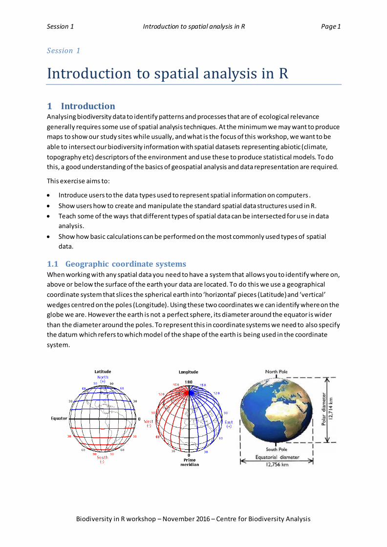
1.1 Geographic coordinate systems When working with any spatial data you need to have a system that allows you to identify where on,

above or below the surface of the earth your data are located. To do this we use a geographical

coordinate system that slices the spherical earth into ‘horizontal’ pieces (Latitude) and ‘vertical’

wedges centred on the poles (Longitude). Using these two coordinates we can identify where on the

globe we are. However the earth is not a perfect sphere, its diameter around the equator is wider

than the diameter around the poles. To represent this in coordinate systems we need to also specify

the datum which refers to which model of the shape of the earth is being used in the coordinate

system.



1.2 Main spatial packages used in R One of the great advantages of R is that it is completely open source software with a very active

development community. This means that for just about any analysis you can think of you can be

reasonably sure that somebody will have written and published a package/function that does it.

While this flexibility is one of the great strengths of R, it can also mean that developers have very

different ideas on data structure.

Developers of spatial analyses in R recognised early on the need for standardised data structures for

spatial information. This would allow any future analyses to become inter-operable, allowing

packages written by different people to be used without having convert your spatial data into

package specific data formats.

The sp package provides these standard data structures, this package also links with several other

open source geospatial libraries, via their R packages, to provide drivers for reading and accessing

different geospatial file formats (GDAL), translations between different coordinate syste ms (GDAL

and proj.4) and spatial geometry calculations (GEOS).

Although sp provides data classes that are excellent for dealing with most spatial data, it still

requires all data to be held in memory meaning that it can struggle when working with large

continuous surfaces (represented as grids), this lead to the raster package which is the primary

package for working with gridded spatial data.

During this session you will need the following R packages installed:

sp, rgdal, rgeos, maptools, fields, rworldmap, dismo, raster, ggmap

If not already installed, you can add them with the following code:

libraries <-

c('sp','rgdal','rgeos','maptools','fields','rworldmap','dismo'

,'raster'. 'ggmap')

install.packages(libraries)



1.3 Getting started To access all the data used in this session you will need to set your working directory to the correct

folder. To set your working directory, use the following code:

wd <- choose.dir() ## select the session 1 'datasets' folder

setwd(wd)

1.4 Representing spatial data on a computer While most spatial information can be stored as familiar data structures (e.g. spread sheets, tables

and arrays) there some standards and conventions to representing real world spatial information on

computers.

There are four main types of spatial data objects which are abstractions of real world information.

Point data are used to represent one, or many, individual locations. For example, these

could be the places where different species were recorded.

Line data are used to represent a continuous trajectory or path such as the foraging

movements of a species.

Polygon data show the boundaries of a closed shape where each shape represent a single

values or unit. For example, country boundaries.

Raster data are used to represent a three dimensional surface where two dimensions

denote the spatial position and the third dimension represents some other value. For

example, average annual temperature across the country.

In the sections below you will learn about how these types of data are stored, manipulated and

plotted in R. Before

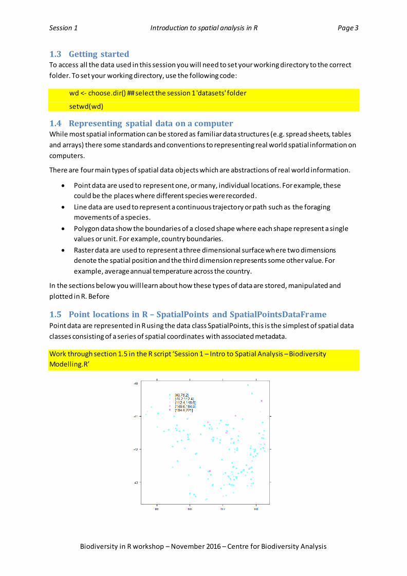
1.5 Point locations in R – SpatialPoints and SpatialPointsDataFrame Point data are represented in R using the data class SpatialPoints, this is the simplest of spatial data

classes consisting of a series of spatial coordinates with associated metadata.

Work through section 1.5 in the R script ‘Session 1 – Intro to Spatial Analysis – Biodiversity

Modelling.R’



1.6 Line data in R – SpatialLines and SpatialLinesDataFrame Line data are slightly more complex than point data, they consist of a series of ordered points that

represent a continuous path between each point. These are handled by the SpatialLines and

SpatialLinesDataFrame classes in R


Modelling.R

1.7 Polygon data in R – SpatialPolygons and SpatialPolygonsDataFrame Polygon data are handled by the data classes SpatialPolygons and SpatialPolygonsDataFrame. These

are structured in a similar way to SpatialLines but instead of representing a continuous path

between points, the points represent the boundary of an object.


Modelling.R’

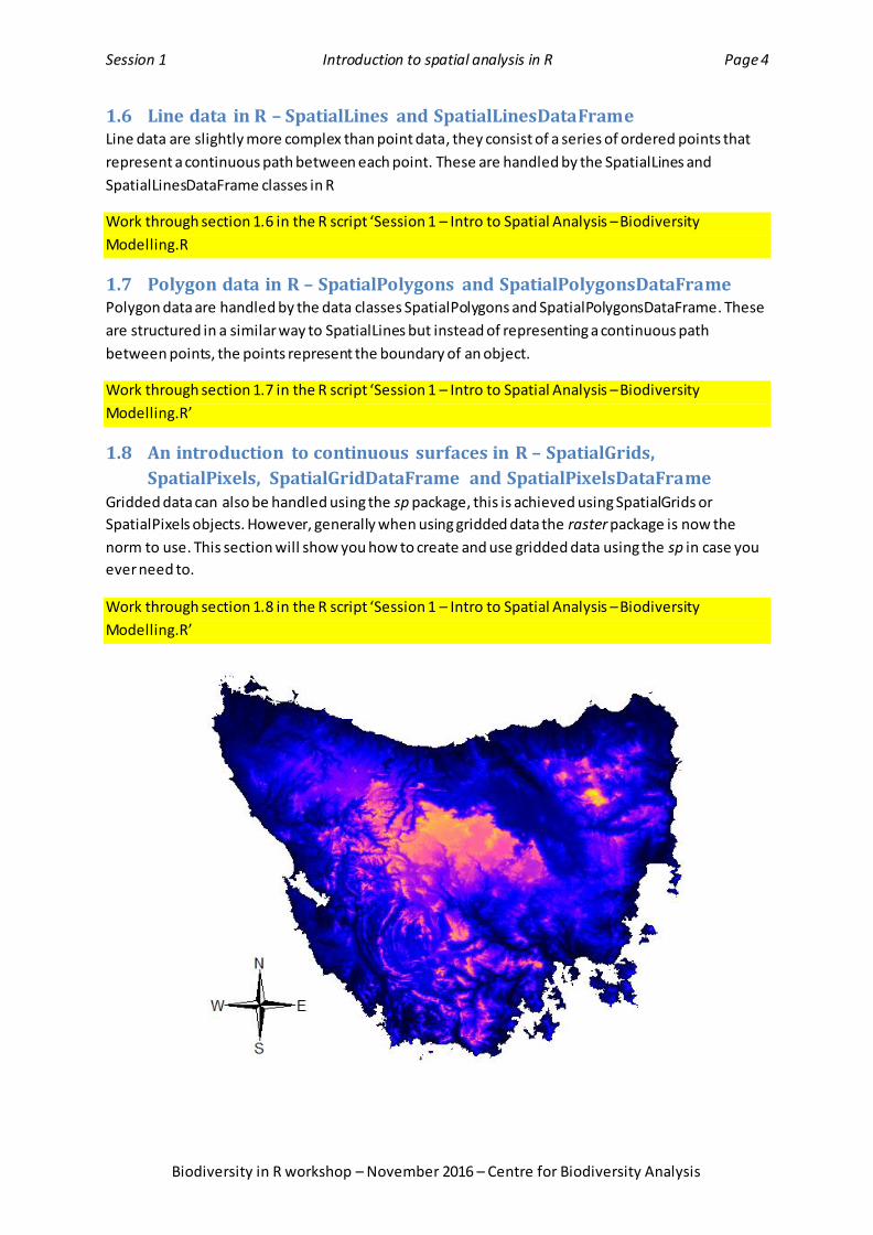
1.8 An introduction to continuous surfaces in R – SpatialGrids,

SpatialPixels, SpatialGridDataFrame and SpatialPixelsDataFrame Gridded data can also be handled using the sp package, this is achieved using SpatialGrids or

SpatialPixels objects. However, generally when using gridded data the raster package is now the

norm to use. This section will show you how to create and use gridded data using the sp in case you

ever need to.


Modelling.R’



1.9 More on geographic coordinate systems – map projections Beyond representing spatial locations as points on the globe, geographers have devised many ways

to represent the globe as a two-dimensional surface that can be displayed as a map or image. To do

this the three dimensional coordinates (Longitude and Latitude) must be projected onto a two

dimensional surface. This projection creates distortions in both distance between points and the

angle between points dependent on where on the globe you are. For example, by mapping longitude

and latitude directly to a planar surface there is extreme distortions of distance at the poles when

compared to the equator.

Geographers deal with this by using map projections. Projections are designed to show the globe, or

parts of the globe, to be as true in either distance or angle (or a trade-off between the two) as

possible. There are numerous map projections and which you use depends on your goal and the

area of the globe you’re working. A good website for more information on map pro jections is

http://egsc.usgs.gov/isb//pubs/MapProjections/projections.html

In R, defining map projections relies on the proj.4 library, using the standards of this library you can

define any projection and transform between them. Depending on the projection a proj.4 string can

have various parts, generally you have to define your projection “+proj=”, the ellipsoid “+ellps=”

and/or the datum “+datum=”. For example the proj.4 string for the WGS84 geographic projection is

"+proj=longlat +ellps=WGS84 +datum=WGS84 +no_defs".

The best way to use proj.4 strings is to determine which projection you require and then look up this

projection on online references to determine the specifics of that projection and how to define it

using a proj.4 string. Some links to useful online references are below.

http://proj4.org/projections/index.html <- This is the proj 4 page

http://www.epsg-registry.org/ <- If you wish to define your projection using the epsg code

http://www.spatialreference.org/ <- this has many useful projection definitions


Modelling.R’.

http://egsc.usgs.gov/isb/pubs/MapProjections/projections.html

http://proj4.org/projections/index.html

http://www.epsg-registry.org/

http://www.spatialreference.org/



1.10 Importing ArcGIS shapefiles into R The rgdal packages provides drivers for reading and writing many of the common spatial data file

types. Using this library, or packages that connect to this library, we are able to import most types of

spatial data that we would encounter. This allows us to import complex spatial objects rather than

having to build them from raw location data ourselves.


Modelling.R’. This will show you a couple of ways to import shape files, as well as building on

previous sections to access parts of the data, transform and plot them.

1.11 Google maps, Open street maps Who doesn’t like a pretty map?


Modelling.R’. This will show you a couple of ways to import and plot map data.



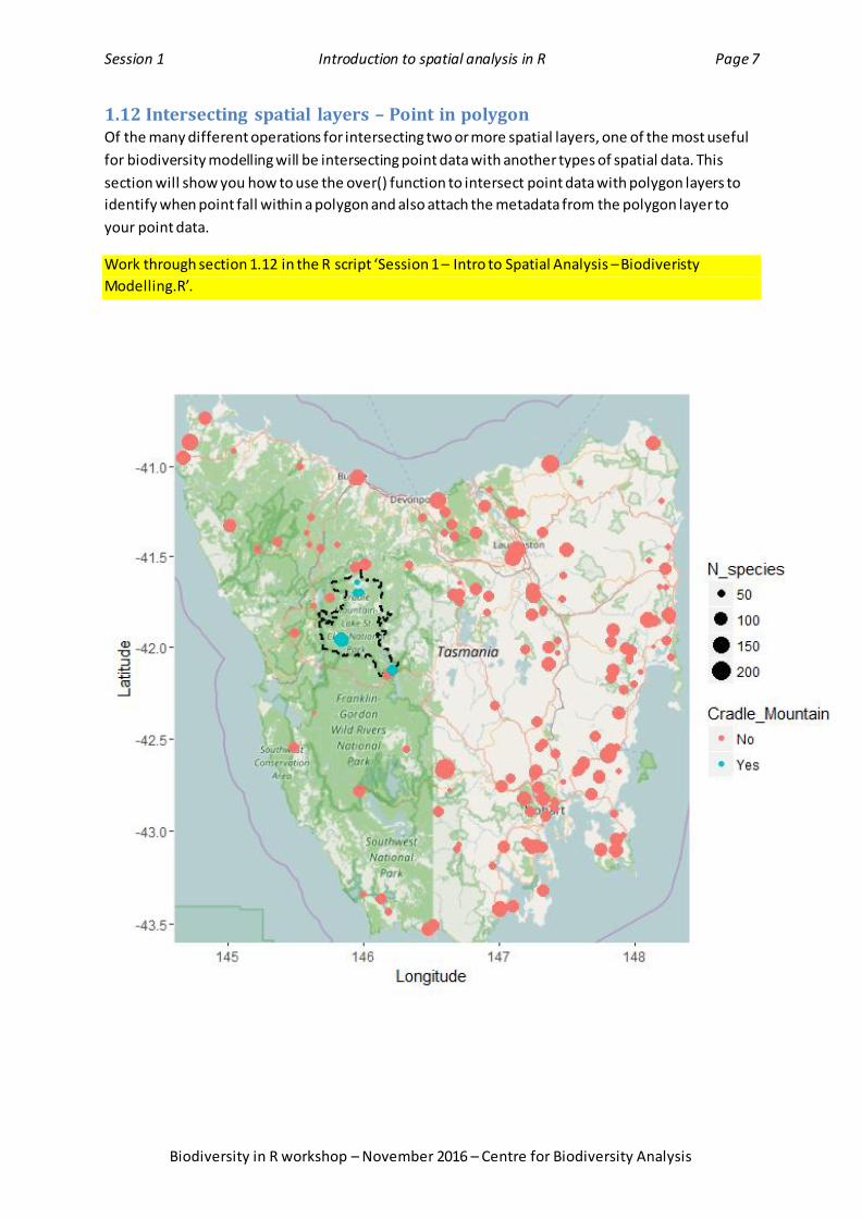
1.12 Intersecting spatial layers – Point in polygon Of the many different operations for intersecting two or more spatial layers, one of the most useful

for biodiversity modelling will be intersecting point data with another types of spatial data. This

section will show you how to use the over() function to intersect point data with polygon layers to

identify when point fall within a polygon and also attach the metadata from the polygon layer to

your point data.

Work through section 1.12 in the R script ‘Session 1 – Intro to Spatial Analysis – Biodiveristy

Modelling.R’.



2 Raster data During this section, we will explore data in raster format, and how we can work with this type of

data in R. A lot of data used in ecological modelling comes in raster format, and the R package

‘raster,’ in particular, provides very user-friendly classes and methods for handling and processing

raster data. See the vignette here:

https://cran.r-project.org/web/packages/raster/vignettes/Raster.pdf

Raster format describes data that is grid of pixels. The pixels are commonly, but not necessarily,

equally spaced. The use of the word ‘pixels’ is borrowed from the world of image files which

commonly also use raster format (e.g. .jpeg, .tif, .png), but when we refer to a ‘geospatial’ raster, we

often use the term ‘cells’ instead of pixels. A geospatial raster has data associated with it encoding

the geographical region depicted by the raster, and the values represent some characteristic of that

region. The geospatial data associated with the grid might be in a separate file (e.g. .flt), or

embedded in the file (e.g. .asc). Minimal associated information required to locate the raster in the

real world is as follows:

Geographical coordinates of a corner (commonly the lower left)

Number of rows and columns

Coordinate reference system.

Important considerations when using raster data in ecological models are the resolution of the data,

and the determining whether different rasters are comparable in terms of their geospatial

attributes. Resolution describes the level of aggregation of raster values, and can be interpreted as

the level of spatial precision (or level of averaging). When using multiple rasters, it is often imp ortant

(or at the very least helpful) if they are spatially comparable. For example, where the land and ocean

are is often not the same in different rasters. We will cover some ways to ‘massage’ rasters so they

become comparable.

While raster data is a commonly used data format for representing gridded spatial data, it isn’t the

only way. Here we’ll also briefly cover how to use another form of commonly used spatial data

(netCDF), and how to use this data format in a raster-based workflow.

To begin, we’ll set up some filepaths to directories that we will work with during the session. Run the

first line of code below to set your working directory. Set this to wherever you have save the folder

‘CAB_COURSE’ (e.g. navigate to the folder 'CBA_COURSE' in the pop-up window).

The raster package holds files (rasters) you are working with in memory in a temporary folder. On

windows, raster will create a folder somewhere like here:

C:\Users\war42q\AppData\Local\Temp\Rtmp21PTuu\raster\ This folder will keeping filling up as you work with more data, and won’t clear until you end the

current R session. So… if you are working with large amounts of data, you will likely want to specify a

different location for raster to hold temporary data.

https://cran.r-project.org/web/packages/raster/vignettes/Raster.pdf



2.1 Raster input In this section we will look at some ways to read in raster data into R, different classes used for

raster data, how to visualise a raster, and how these are stored in memory.

Work through section 2.1 in the R script ‘Session 1 – Intro to raster.’

2.2 Accessing raster properties Here we will look at global and cell-based properties of rasters. In this section we will cover how to

get values out of a raster at particular locations, and digress into the slightly off -topic – but relevant -

exercise of obtaining biological spatial occurrence data from within R. We will get data from GBIF

and the ALA, but the purpose is to expose you to the packages which interact with both databases,

rather than go into detail of the extensive functionality provided.


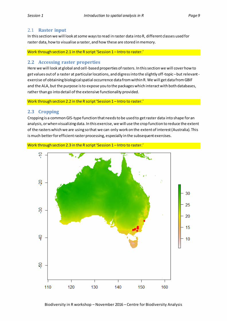
2.3 Cropping Cropping is a common GIS-type function that needs to be used to get raster data into shape for an

analysis, or when visualizing data. In this exercise, we will use the crop function to reduce the extent

of the rasters which we are using so that we can only work on the extent of interest (Australia). This

is much better for efficient raster processing, especially in the subsequent exercises.




2.4 Working with raster values: math and indexing The ease with which you can perform calculations on rasters in the raster package is one of its

strengths. Here we will go through a few simple exercises to demonstrate how you can do ‘raster

math’ and use indexing to modify values.


2.5 Creating rasters There are several ways to create raster data depending on the data from which it is created. Here,

the exercises will demonstrate how to create a dummy raster in R, a raster from points, a raster

from a vector format, and assign and modify spatial information associated with raster.


2.6 Projection Building from the previous section on vector data, we will look here at how projection information is

handled for raster data.


2.7 Writing rasters to disk Here, the exercises will cover how to save raster files to your computer. We will look at different file

and data types, and some important parameters to consider when writing rasters to disk (especially

if the rasters will be used in other software).


2.8 Working with netCDF netCDF files are a common data format used, especially for any sort of climate data. They come into

their own where data which has greater than three dimensions needs to be stored.

ncdf packages, but also the raster package, provide classes and methods for working with netCDF

data. Given our focus here is on raster data, we will look at ways to work with netCDF files in a

raster-based workflow. Given many common tasks performed when setting up to data to use in



models are catered to so well by the raster package, handling netCDF data as raster data may often

be the simplest.


2.9 Making rasters align (stack) The exercises in this section focus on a few ways force different rasters to be spatially consistent.

This often involves modifying the data in some way, so it is important that what you are doing when

massaging data into shape is well understood!


2.10 Masking Masking a raster by values (or no data values) in another raster is a common GIS-type function which

we often need to perform. Here we will simply mask areas (i.e. convert to no data) in an

environmental variable which are not in the protected areas raster which we created above.


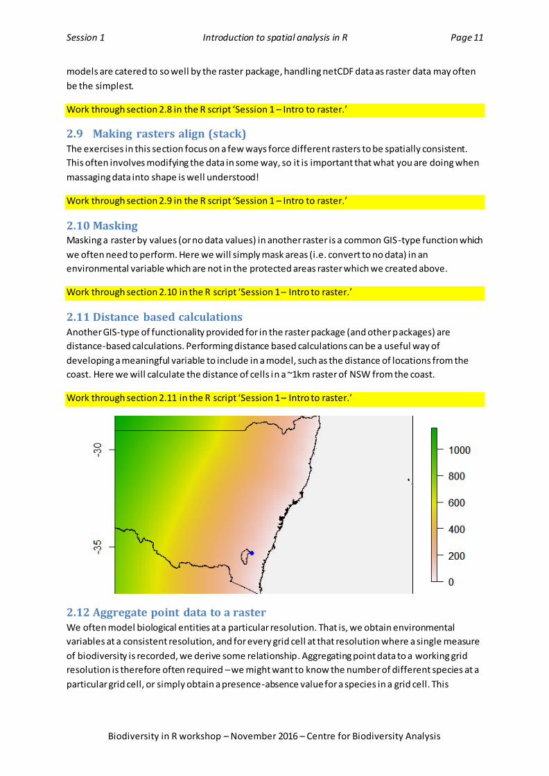
2.11 Distance based calculations Another GIS-type of functionality provided for in the raster package (and other packages) are

distance-based calculations. Performing distance based calculations can be a useful way of

developing a meaningful variable to include in a model, such as the distance of locations from the

coast. Here we will calculate the distance of cells in a ~1km raster of NSW from the coast.


2.12 Aggregate point data to a raster We often model biological entities at a particular resolution. That is, we obtain environmental

variables at a consistent resolution, and for every grid cell at that resolution where a single measure

of biodiversity is recorded, we derive some relationship. Aggregating point data to a working grid

resolution is therefore often required – we might want to know the number of different species at a

particular grid cell, or simply obtain a presence-absence value for a species in a grid cell. This



exercise will cover one way of achieving this, and plotting the output to visualise the effect of

aggregating biological occurrence data.


2.13 Zonal statistics. Obtaining summary statistics over some region is often useful when preparing inputs for a model, or

perhaps more so, when summarizing results of a model. The zonal statistics function allows us to do

this with raster data.


2.14 Rasters and model predictions Here, we will go through an exercise of fitting a model to some occurrence records and

environmental data, and then obtaining predictions based on that across a raster surface for an

entire region (Tasmania). We’ll use environmental raster data already loaded in memory, and a .csv

file of (fabricated) presence/absence data. This isn’t a community model exercise… but instead a

(hopefully) simple exercise in generating predictions for a raster surface.




2.15 Many more relevant functions available... So far, we have only scraped the surface of what the raster package (and other packages in R) are

capable of doing. Hopefully, we have covered the most-common tasks required when working with

raster data in a modelling workflow.


2.16 (brief) plotting section Plotting and creating figures/mapped outputs is an entire course on its own. It’s possible to spend a

large amount of a PhD/postdoc finessing figures – these exercises won’t help with this, sorry! The

first two exercises in this section are basic, and just demonstrate how to change a colour ramp in

raster plot (a common task), and how to write an image file to disk. The second two are by no means

exhaustive, but are just mean to demonstrate two extensions of figure generation/mapping over the

base functions using raster data – just to demonstrate some of what is possible. These will introduce

you to plotting in an additional graphics package (ggplot2) and how to create an interactive map.




3 Some places to get spatial information – Biological and

Environmental Species records: Atlas of Living Australia: www.ala.org.au There is an additional exercise showing you some of the ways the ALA4R package can be used to

access species records from the Atlas of Living Australia via R. If you have time – or feel free to do it

later – work through the script ‘ALA4R_example.R’

Global Biodiversity Information Facility: www.gbif.org OBIS seamap: www. http://seamap.env.duke.edu/

Map of Life: https://mol.org/

Environmental data:

WorldClim: http://www.worldclim.org/

AnuClim: http://fennerschool.anu.edu.au/research/products

Global substrate info: https://soilgrids.org/

Australian soil data: http://www.clw.csiro.au/aclep/soilandlandscapegrid/

Australian land-cover: http://www.ga.gov.au/scientific-topics/earth-obs/landcover

Global 1km land cover, habitat heterogeneity, cloud cover and more: http://www.earthenv.org/

Anthropogenic data:

Protected planet for global protected areas layer: www.protectedplanet.net

CAPAD for Australian protected area layers:

http://www.environment.gov.au/land/nrs/science/capad

http://www.ala.org.au/

http://www.gbif.org/

http://seamap.env.duke.edu/

https://mol.org/

http://www.worldclim.org/

http://fennerschool.anu.edu.au/research/products

https://soilgrids.org/

http://www.clw.csiro.au/aclep/soilandlandscapegrid/

http://www.ga.gov.au/scientific-topics/earth-obs/landcover

http://www.earthenv.org/

http://www.protectedplanet.net/

http://www.environment.gov.au/land/nrs/science/capad

session 1 introduction to spatial analysis in...

Documents