serum biomarkers: promising tool for predicting … · 2/26/2015 · serum biomarkers: promising...

Lab in Statistical Design and Analysis

Final Lab Report

Serum Biomarkers: Promising Tool for Predicting Survival and

Tumor Response in Malignant Mesothelioma

Abstract

Introduction

Malignant Mesothelioma (MM) is an aggressive form of cancer with median survival less than 1

year. The number of MM cases has risen steadily over the past two decades. Radiologic

assessment of the tumor response for MM is difficult, therefore researchers are trying to

identify an alternative approach to monitor tumor response. In this study, we are interested in

using serum biomarkers (CA125, SMRP, MPF and CYFRA) as a tool to monitor tumor response

and predict survival outcome.

Methods

Data from patients diagnosed with MM between 2005 and 2010 at the University Health

Network were collected retrospectively from chart review. Baseline biomarkers values and

other covariates were used in survival analysis. Tumor response between pre and post

treatment, showing progression, stable and response were compared to corresponding changes

in the biomarkers values.

Results

Seventy-three patients (median age: 64 years old (range: 29-83)) were included in the overall survival

analysis with median follow-up time of 1.1 years (range: 0.05 – 3.5). Forty-four patients were

deceased and 29 still alive. The median survival was 1.5 years. Multi-variate analysis indicated

that the biomarker CYFRA (p=0.0005), baseline platelet (p=0.0012) and surgery (p=0.0004) were

predictive of survival. Associations were identified for biomarker CYFRA (p=0.037) and SMPR

(p=0.04) with the tumor response for patients treated with chemotherapy. No association was

observed for biomarker MPF and CA125.

Conclusion

Baseline CYFRA, platelet and surgery are potential predictors for survival outcome. Percentage

change or difference in SMRP or CYFRA pre and post treatment are potential useful markers of

tumor response. A prospective study with larger sample is recommended to validate the

findings in this study.

Table of Content

Abstract ----------------------------------------------------------------------------------------------------------------------------- 2

Table of Content ------------------------------------------------------------------------------------------------------------------ 3

Introduction ----------------------------------------------------------------------------------------------------------------------- 4

Materials and Methods --------------------------------------------------------------------------------------------------------- 5

1. Study Design/Population --------------------------------------------------------------------------------------------- 5

1.1 Study participants ------------------------------------------------------------------------------------------------ 5

1.2 Variable ------------------------------------------------------------------------------------------------------------- 6

2. Outcome ------------------------------------------------------------------------------------------------------------------ 7

3. Statistical Analysis ------------------------------------------------------------------------------------------------------ 7

3.1 Overall Survival --------------------------------------------------------------------------------------------------- 7

3.2 Association between the difference or percentage change in the pre and post values of the

biomarkers CA125, CYFRA, SMRP and MPF and the tumor response in each type of treatment ------ 8

4. Software ------------------------------------------------------------------------------------------------------------------ 8

Results ------------------------------------------------------------------------------------------------------------------------------- 9

5.1 Overall Survival ------------------------------------------------------------------------------------------------------ 9

5.2 Association between the difference or percentage change in the pre and post values of the

biomarkers CA125, CYFRA, SMRP and MPF and the response in each type of treatment ----------------- 13

Discussion ------------------------------------------------------------------------------------------------------------------------- 17

Conclusion ------------------------------------------------------------------------------------------------------------------------- 19

Reference-------------------------------------------------------------------------------------------------------------------------- 20

Appendices ------------------------------------------------------------------------------------------------------------------------ 21

A. Tables --------------------------------------------------------------------------------------------------------------------- 21

B. Figures -------------------------------------------------------------------------------------------------------------------- 23

SAS codes -------------------------------------------------------------------------------------------------------------------------- 48

4 | P a g e

Introduction

Asbestos, a silicate mineral which is resistant to fire and heat, is often used as electrical

insulation for hotplate wiring and in building insulation. It has been mined and exported from

Canada for centuries. Although asbestos has lucrative commercial qualities, it is carcinogenic.

Since 1960, industrial exposure to asbestos has led to a dramatic rise in the number of cases of

malignant mesothelioma (MM). MM is a rare form of cancer that affects the thin membrane of

the mesothelium (lining of lung, heart and abdomen). Malignant mesothelioma is highly

aggressive with median survival less than 1 year. Symptoms may not appear 20-50 years after

exposure. In Canada, the rate of diagnosed mesothelioma cases has risen steadily over the

past two decades, from 153 cases in 1984 to 344 cases in 20036.

Malignant mesothelioma does not usually grow spherically, rather as an increased

thickening of the pleural rind. Therefore, it is difficult to monitor the response to treatment for

MM patients. Non-invasive biomarker, which is defined as a characteristic that can be

objectively measured and evaluated as an indicator of normal and disease processes or

pharmacological responses5, have been widely used to predict, detect and monitor cancer

disease. Several immunohistochemical markers have been identified as a useful tool to monitor

the response. In this study, we are interested in using serum biomarkers as a tool to monitor

the response to treatment and predict survival outcome.

The four candidate serum biomarkers examined in this study are i) Cancer Antigen 125

(CA125), ii) Soluable mesothelin-related peptide (SMRP), iii) soluble cytokeratin 19 fragment

(CYFRA) and iv) megakaryocyte potentiating factor (MPF). These biomarkers are proteins found

5 | P a g e

on the surface of the cancerous cells. Previous studies have indicated that increased levels of

these biomarkers have a positive correlation with the metastases, tumor progression and

invasion. The two main objectives of this study are to examine the relationship between the

biomarkers and overall survival, as well as how the changes in values of the biomarkers related

to response to treatment (i.e. progression, response or stable).

As workplace exposure to asbestos continues in Canada, primarily in the mining and

construction sectors, it is important to identify non-invasive biological tools which can be used

to monitor or detect the disease so patient’s quality of life and life expectancy can be extended.

It will have positive impact on patients’ health as well as the economy, as billions of dollars will

be saved in treatment and compensation.

Materials and Methods

1. Study Design/Population

1.1 Study participants

This is a single institute retrospective chart-review study, which 117 UHN (University Health

Network) patients diagnosed with MM between 2005 and 2010 were included in the study.

Patients’ information was collected from clinical records, radiotherapy, surgical, pathology and

pharmacy records and recorded in MS Access database. No a priori calculation on sample size

was done and all available patients satisfied the above criteria were included.

In order to qualify for the survival analysis, a patient must have baseline biomarker values

obtained within 3 months of diagnosis and follow up data. For the analysis on response to

treatment, patients must have a pair of measurements pre and post treatment. Biomarker

6 | P a g e

values and CT scan results must be obtained both pre and post treatment. The pre-treatment

biomarker values must be within 1 month of the pre-treatment CT scan, same criteria apply for

the post-treatment.

1.2 Variable

The main variables of interest are the four biomarkers CA125, SMRP, CYFRA and MPF. Those

values were captured as continuous variables. For survival analysis, follow-up time

(continuous) was calculated from date of diagnosis to the last follow up date for alive patients,

and date of death for deceased patients. Covariates were examined in both uni-variate and

multi-variate survival analyses. Categorical covariates were sex (M/F), stage (1-4), thorax

involved (Y/N), histological subtype (epitheliod/biphasic), surgery (Y/N), ECOG (0/0+),

chemotherapy (Y/N), white cell count (≤8.3/>8.3), haemoglobin (≤140/>140), platelet count

(≤400/>400), chest pain (Y/N), weight loss (Y/N), smoking status (current/former/never).

Continuous covariate was age at diagnosis (calculated from date of diagnosis and date of birth).

For the analysis on response to treatment, radiological stage of the response was assessed

using the modified Response Evaluation Criteria In Solid Tumors (mRECIST), which measure

pleural tumor thickness perpendicular to the chest wall at three separate levels. CT scan was

obtained pre and post treatment, the change in tumor was classified as response (>30%

decrease in size), stable or progression (>20% increase in size). Difference and percentage

change were calculated from pre and post measurements of the four biomarkers. Difference

was calculated from subtracting the pre from the post measurement. Percentage change was

calculated from subtracting the pre from the post measurement then divided by the pre

treatment measurement. Missing data could not be imputed, they were treated as missing.

7 | P a g e

2. Outcome

There are two outcomes of interest i) Overall survival analysis ii) the association between the

difference or percentage change in the pre and post values of the biomarkers CA125, CYFRA,

SMRP and MPF and the tumor response in each type of treatment (chemotherapy, best

supportive care (BSC) and radiation). The difference and percentage change were used

because these are the two clinical standards that the clinicians were interested in to examine

the changes. Also clinicians were trying to mimic the analyses that were done in an earlier

study7.

3. Statistical Analysis

3.1 Overall Survival

Kaplan-Meier (non-parametric) and Cox proportional hazard (semi-parametric) were used for

the analyses. A patient had an event if the patient deceased. The follow-up time and the

covariates used in the analysis were provided in section 1.1. Uni-variate analyses on the 18

covariates were performed. Purposeful selection of covariates was used to select covariates for

the multi-variate model. Variables which were significant in the uni-variate model were

included in the multi-variate model. The variables that were significant in the new model

remained in the model and the ones that were not significant were removed. The remaining

variables (which were not significant in the uni-variate analysis) were added one by one to

decide the final model. The Cox proportional hazard assumption was tested by introducing

interaction between the covariate and the log of follow-up time. If the p-value of the

interaction term is not significant, the Cox proportional hazard assumption is not violated.

Interactions between the covariates in the final multi-variate model were examined. The

8 | P a g e

martingale residuals and deviance residuals were used to access the goodness of fit of the final

model.

3.2 Association between the difference or percentage change in the pre and

post values of the biomarkers CA125, CYFRA, SMRP and MPF and the tumor

response in each type of treatment

Box plots and waterfall plots were created to explore the difference and percentage change in

the biomarkers in each treatment group. Krustal-Wallis non-parametric test was used to

compare the difference or percentage change in the pre and post values of the biomarkers and

the response to treatment (progression, stable and response) in the chemotherapy group.

Wilcoxin-Mann-Whitney non-parametric test was used for the treatment group Best-

Supportive-Care because there were only two response types (progression and stable). There

were only a few patients in the radiation group, no analysis was carried out. Recognizing there

are other methodologies such as ANCOVA that can be used for the analysis, based on the

constraint to mimic analyses done in a previous study mentioned above, the described

methodologies were chosen. Correlation between the four biomarkers was evaluated using

spearman’s rank correlation coefficient.

4. Software

The SAS procedures: proc means, proc univariate, proc freq, proc npar1way, proc lifetest and

proc tphreg were used to carry out the statistical analysis. All analyses were performed using

SAS v9.1 for windows and all reported p-values were 2-sided. P-value < 0.05 was considered

significant. Reported p-values will not be adjusted for multiple testing; results should be

interpreted with caution.

9 | P a g e

Results

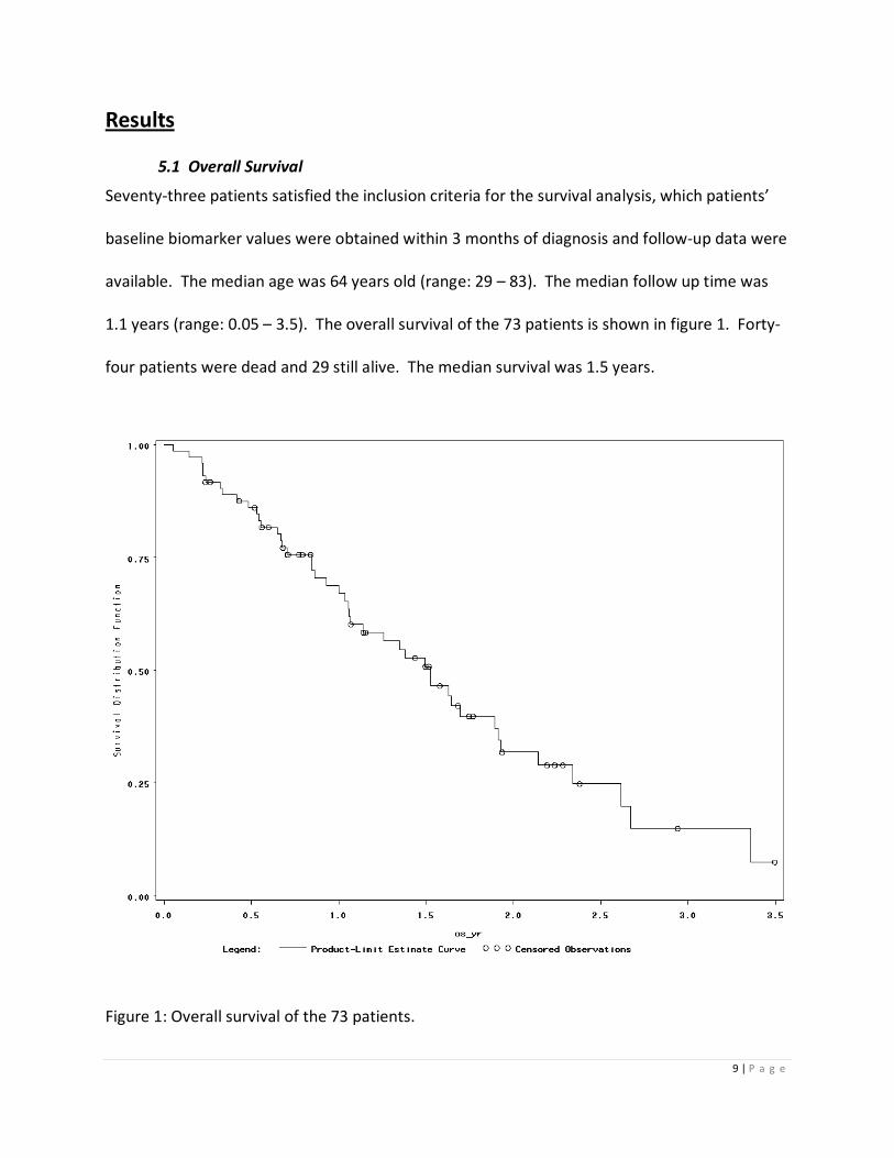
5.1 Overall Survival

Seventy-three patients satisfied the inclusion criteria for the survival analysis, which patients’

baseline biomarker values were obtained within 3 months of diagnosis and follow-up data were

available. The median age was 64 years old (range: 29 – 83). The median follow up time was

1.1 years (range: 0.05 – 3.5). The overall survival of the 73 patients is shown in figure 1. Forty-

four patients were dead and 29 still alive. The median survival was 1.5 years.

Figure 1: Overall survival of the 73 patients.

10 | P a g e

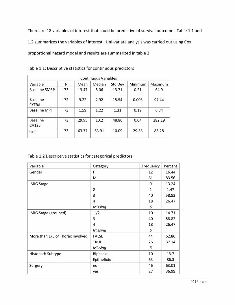
There are 18 variables of interest that could be predictive of survival outcome. Table 1.1 and

1.2 summarizes the variables of interest. Uni-variate analysis was carried out using Cox

proportional hazard model and results are summarized in table 2.

Table 1.1: Descriptive statistics for continuous predictors

Continuous Variables

Variable N Mean Median Std Dev Minimum Maximum

Baseline SMRP 73 13.47 8.06 13.71 0.21 64.9

Baseline

CYFRA

72 9.22 2.92 15.54 0.003 97.44

Baseline MPF 73 1.59 1.22 1.31 0.19 6.34

Baseline

CA125

73 29.95 10.2 48.86 0.04 282.19

age 73 63.77 63.91 10.09 29.33 83.28

Table 1.2 Descriptive statistics for categorical predictors

Variable Category Frequency Percent

Gender F 12 16.44

M 61 83.56

IMIG Stage 1 9 13.24

2 1 1.47

3 40 58.82

4 18 26.47

Missing 5

IMIG Stage (grouped) 1/2 10 14.71

3 40 58.82

4 18 26.47

Missing 5

More than 1/3 of Thorax Involved FALSE 44 62.86

TRUE 26 37.14

Missing 3

Histopath Subtype Biphasic 10 13.7

Epithelioid 63 86.3

Surgery no 46 63.01

yes 27 36.99

11 | P a g e

Chest Pain No 22 42.31

Yes 30 57.69

Missing 21

Weight Loss No 25 40.32

Yes 37 59.68

Missing 11

ECOG 0 37 50.68

1 27 36.99

2 5 6.85

3 4 5.48

ECOG (grouped) 0 37 50.68

1/2/3 36 49.32

Smoking Status Current 9 13.43

Former (>1 yr) 3 4.48

Former (>1 yr) Pack

years- 1 1.49

Never 32 47.76

former (>1 yr) 22 32.84

Missing 6

Smoking Status (grouped) never 32 47.76

former 26 38.81

current 9 13.43

Missing 6

Chemotherapy Yes 47 64.38

no 26 35.62

White Cell Count ≤ 8.3 37 60.66

> 8.3 24 39.34

Missing 12

Platelet ≤ 400 41 66.13

> 400 21 33.87

Missing 11

Haemoglobin ≤ 140 41 66.13

> 140 21 33.87

Missing 11

12 | P a g e

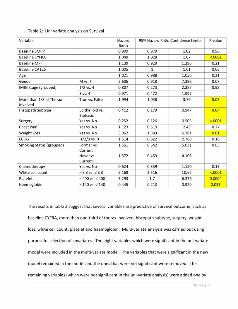
Table 2: Uni-variate analysis on Survival

Variable Hazard

Ratio

95% Hazard Ratio Confidence Limits P-value

Baseline SMRP 0.999 0.979 1.02 0.96

Baseline CYFRA 1.049 1.028 1.07 <.0001

Baseline MPF 1.139 0.929 1.396 0.21

Baseline CA125 1.005 1 1.01 0.06

Age 1.021 0.988 1.056 0.21

Gender M vs. F 2.606 0.918 7.396 0.07

IMIG Stage (grouped) 1/2 vs. 4 0.807 0.273 2.387 0.92

3 vs. 4 0.971 0.472 1.997

More than 1/3 of Thorax

Involved

True vs. False 1.994 1.058 3.76 0.03

Histopath Subtype Epithelioid vs.

Biphasic

0.412 0.179 0.947 0.04

Surgery Yes vs. No 0.252 0.126 0.503 <.0001

Chest Pain Yes vs. No 1.123 0.519 2.43 0.77

Weight Loss Yes vs. No 3.062 1.383 6.781 0.01

ECOG 1/2/3 vs. 0 1.514 0.822 2.788 0.18

Smoking Status (grouped) Former vs.

Current

1.651 0.542 5.031 0.65

Never vs.

Current

1.372 0.459 4.106

Chemotherapy Yes vs. No 0.624 0.339 1.150 0.13

White cell count > 8.3 vs. ≤ 8.3 5.169 2.516 10.62 <.0001

Platelet > 400 vs. ≤ 400 3.293 1.7 6.376 0.0004

Haemoglobin > 140 vs. ≤ 140 0.445 0.213 0.929 0.031

The results in table 2 suggest that several variables are predictive of survival outcome, such as

baseline CYFRA, more than one-third of thorax involved, histopath subtype, surgery, weight

loss, white cell count, platelet and haemoglobin. Multi-variate analysis was carried out using

purposeful selection of covariates. The eight variables which were significant in the uni-variate

model were included in the multi-variate model. The variables that were significant in the new

model remained in the model and the ones that were not significant were removed. The

remaining variables (which were not significant in the uni-variate analysis) were added one by

13 | P a g e

one to decide the final model. Table 3 presents the results for the multi-variate model. For

every unit increases in baseline CYFRA, the risk for event of death increases by 4%. The group

with platelet > 400 has 3 times the risk to experience of outcome of death whereas the group

with surgery has lower risk compare to the group without surgery. Interactions of the variables

in table 3 were examined and results are provided in Appendix A1. The proportional hazard

assumption was tested by introducing interaction between the covariate and the log of follow-

up time, results provided in Appendix A2. The goodness of fit of the model was examined using

martingale residuals and deviance residuals. The results are provided in Appendix B1 and B2.

The goodness of fit indicated this multi-variate model was suitable.

Table 3: Multi-variate analysis on Survival

Variable Hazard

Ratio

95% Hazard Ratio Confidence Limits P-value

Baseline CYFRA 1.04 1.02 1.07 0.0005

Platelet > 400 vs. ≤ 400 3.29 1.6 6.8 0.0012

Surgery Yes vs. No 0.22 0.1 0.5 0.0004

5.2 Association between the difference or percentage change in the pre and post

values of the biomarkers CA125, CYFRA, SMRP and MPF and the response in each

type of treatment

There were 104 patients satisfied the inclusion criteria and were included in this analysis. All of

these patients have a pair of pre and post treatment blood measurement and CT scan. Also the

blood measurements were obtained within 1 month from the CT scan. The analysis was carried

out separately for each of the treatment group (i.e. chemotherapy, best supportive care and

radiation). Table 4 summarizes the number of patients included in the analysis for each of the

treatment group. There were only 7 patients in the radiation group, therefore analysis was

deemed unsuitable and only exploratory work such as box plots and waterfall plots were

14 | P a g e

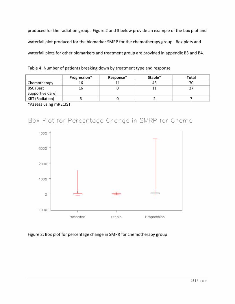
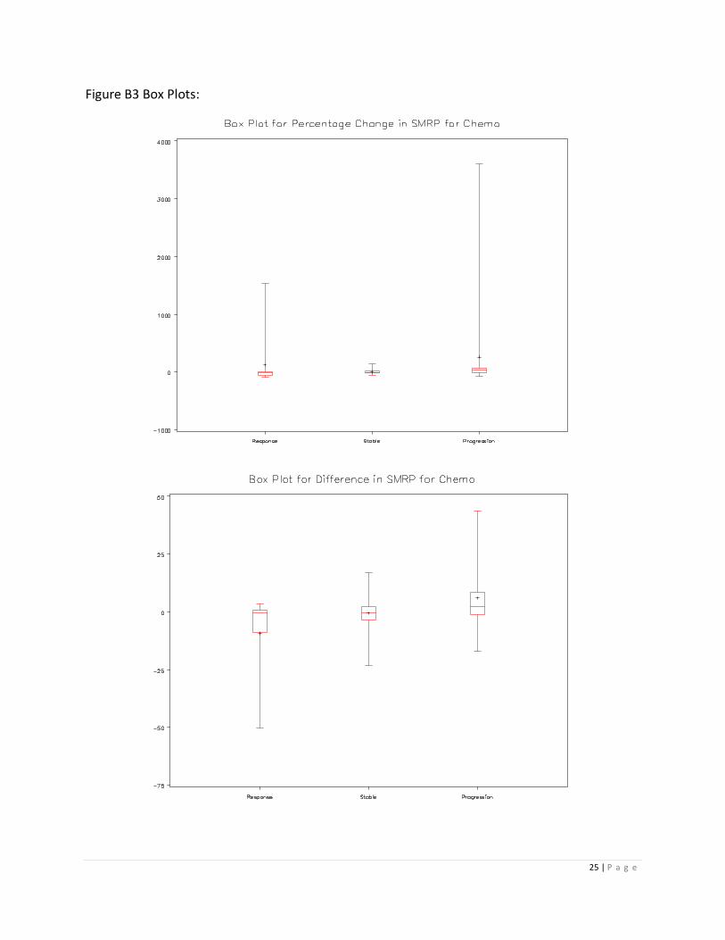
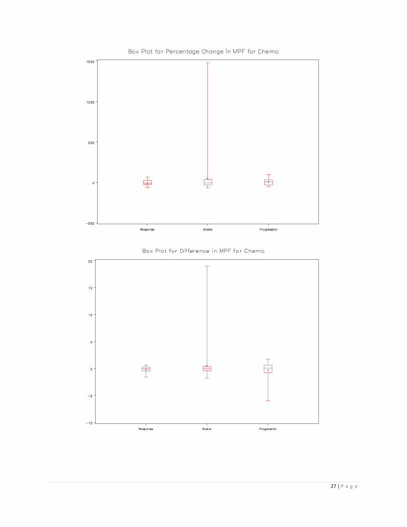
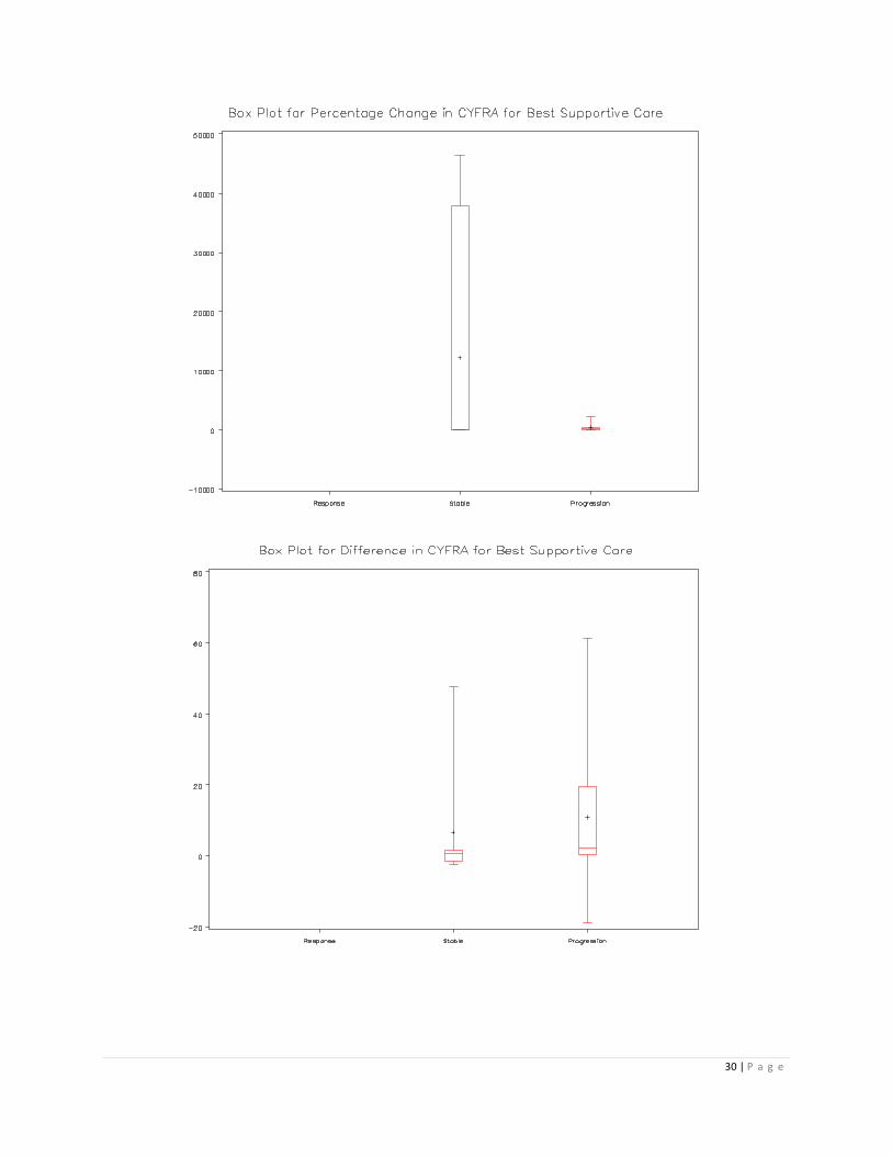
produced for the radiation group. Figure 2 and 3 below provide an example of the box plot and

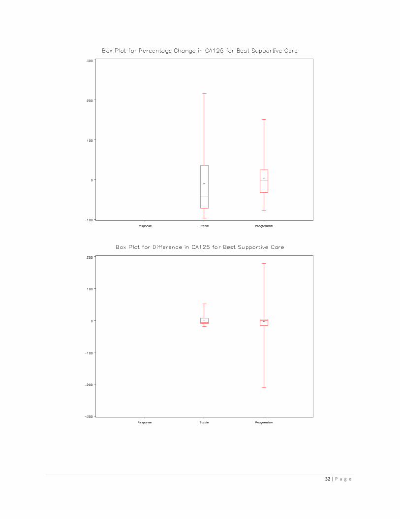
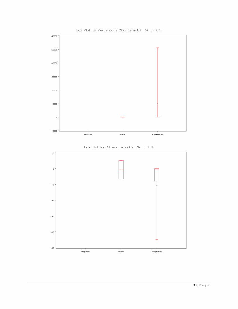
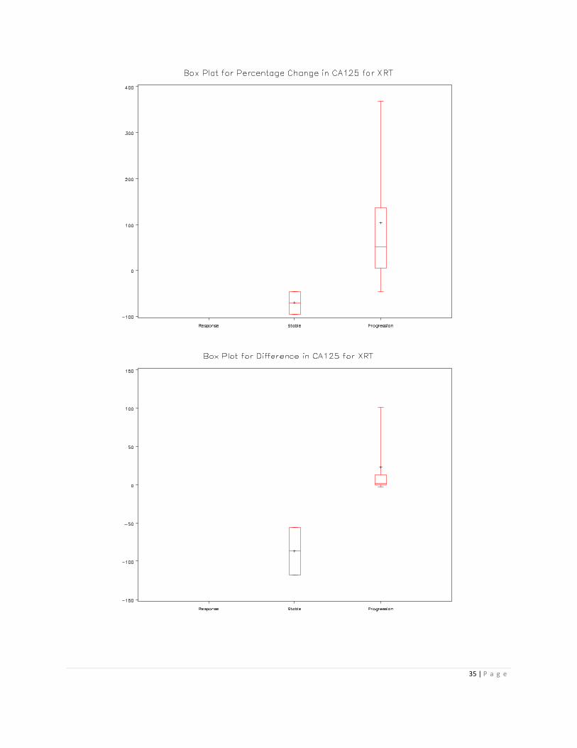
waterfall plot produced for the biomarker SMRP for the chemotherapy group. Box plots and

waterfall plots for other biomarkers and treatment group are provided in appendix B3 and B4.

Table 4: Number of patients breaking down by treatment type and response

N=104 Progression* Response* Stable* Total

Chemotherapy 16 11 43 70

BSC (Best

Supportive Care)

16 0 11 27

XRT (Radiation) 5 0 2 7

*Assess using mRECIST

Figure 2: Box plot for percentage change in SMPR for chemotherapy group

15 | P a g e

05

00

15

00

25

00

35

00

StableResponse

Progression

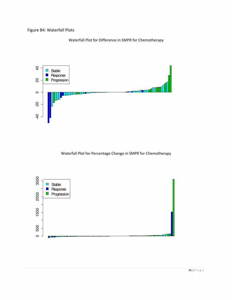
Figure 3: Waterfall plot for percentage change in SMPR for chemotherapy group

As one can observed in figure 2 and 3, there are some outliers for the percentage change and

the difference. Those outliers have been verified with the clinician to ensure data accuracy.

Non-parametric test such as Krustal-Wallis and Wilcoxin-Mann-Whitney were employed for the

analysis which utilizes the rank, transformation was not applied to data. Descriptive statistics of

the difference and percentage change of the four biomarkers are presented in table 5 for the

chemotherapy group and table 6 for the best supportive care group. The descriptive statistics

for the radiation group is provided in appendix A3.

16 | P a g e

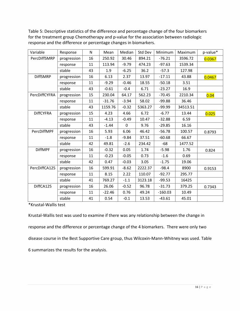
Table 5: Descriptive statistics of the difference and percentage change of the four biomarkers

for the treatment group Chemotherapy and p-value for the association between radiologic

response and the difference or percentage changes in biomarkers.

Variable Response N Mean Median Std Dev Minimum Maximum p-value*

PercDiffSMRP progression 16 250.92 30.46 894.21 -76.21 3596.72 0.0367

response 11 113.94 -9.79 474.23 -97.63 1539.34

stable 43 1.9 -6.25 36.2 -57.3 127.98

DiffSMRP progression 16 6.13 2.37 13.97 -17.11 43.88 0.0467

response 11 -9.29 -0.46 18.55 -50.18 3.51

stable 43 -0.61 -0.4 6.71 -23.27 16.9

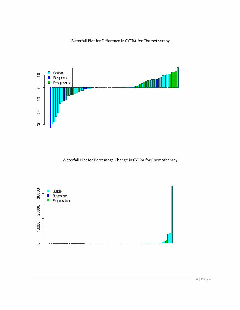
PercDiffCYFRA progression 15 230.04 64.17 562.23 -70.45 2210.34 0.04

response 11 -31.76 -3.94 58.02 -99.88 36.46

stable 43 1159.76 -0.32 5363.27 -99.99 34513.51

DiffCYFRA progression 15 4.23 4.66 6.72 -6.77 13.44 0.025

response 11 -4.13 -0.49 10.47 -32.88 6.59

stable 43 -1.44 0 9.76 -29.85 16.16

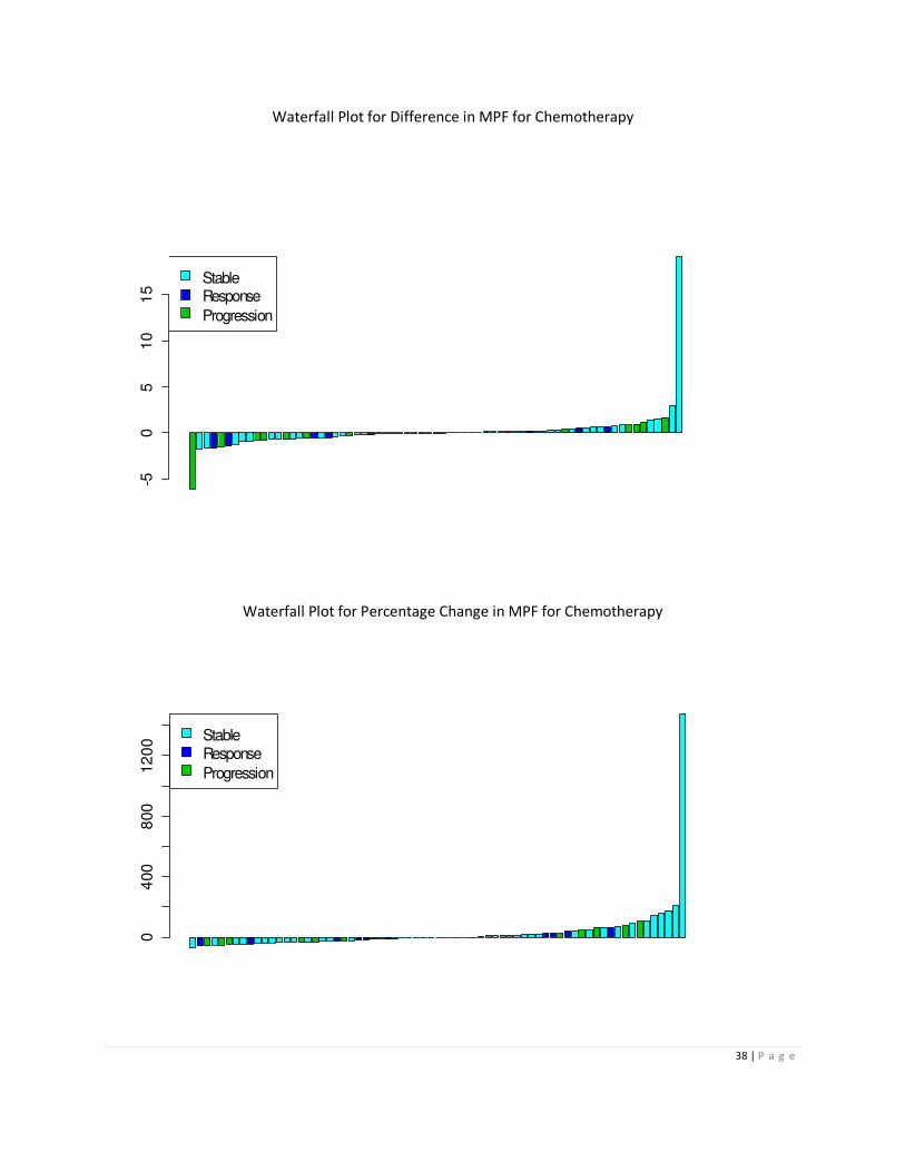
PercDiffMPF progression 16 5.93 6.06 46.42 -56.78 100.57 0.8793

response 11 -1.8 -9.84 37.51 -60.68 66.67

stable 42 49.81 -2.6 234.42 -68 1477.52

DiffMPF progression 16 -0.32 0.05 1.74 -5.98 1.76 0.824

response 11 -0.23 -0.05 0.73 -1.6 0.69

stable 42 0.47 -0.03 3.05 -1.75 19.06

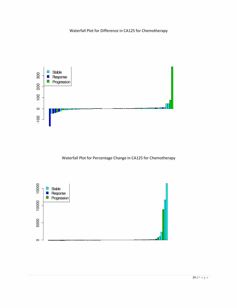
PercDiffCA125 progression 16 599.91 -8.62 2222.37 -98.4 8900 0.9153

response 11 8.15 2.22 110.07 -92.77 295.77

stable 41 769.27 -1.1 3123.18 -99.53 16425

DiffCA125 progression 16 26.06 -0.52 96.78 -31.73 379.25 0.7343

response 11 -22.46 0.76 49.24 -160.03 10.49

stable 41 0.54 -0.1 13.53 -43.61 45.01

*Krustal-Wallis test

Krustal-Wallis test was used to examine if there was any relationship between the change in

response and the difference or percentage change of the 4 biomarkers. There were only two

disease course in the Best Supportive Care group, thus Wilcoxin-Mann-Whitney was used. Table

6 summarizes the results for the analysis.

17 | P a g e

Table 6: Descriptive statistics of the difference and percentage change of the four biomarkers

for the treatment group Best Supportive Care and p-value for the association between

radiologic response and the difference or percentage changes in biomarkers.

Variable Response N Mean Median Std Dev Minimum Maximum p-value*

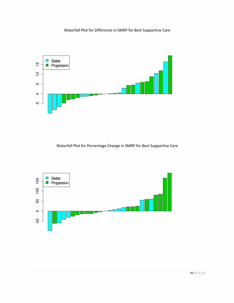
PercDiffSMRP progression 16 31.4 10.7 68.72 -59.88 189.17 0.2669

stable 11 -6.49 3.79 46.79 -95.41 60.48

DiffSMRP progression 16 2.97 0.16 6.37 -4.7 19.4 0.5053

stable 11 0.83 0.1 7.87 -9.8 16.42

PercDiffCYFRA progression 16 408.39 142.73 653.54 -92.24 2263.64 0.8243

stable 11 12206 46.15 19796.9 -82.58 46400

DiffCYFRA progression 16 10.86 1.97 21.71 -18.78 61.23 0.1748

stable 11 6.55 0.76 15.86 -2.6 47.72

PercDiffMPF progression 16 41.01 33.17 56.89 -46.05 176.26 0.1201

stable 11 9.98 6.14 37.28 -36.82 97.3

DiffMPF progression 16 0.55 0.16 0.95 -0.7 2.67 0.2361

stable 11 0.04 0.06 0.48 -1.09 0.72

PercDiffCA125 progression 16 4.28 -1.45 54.92 -77.56 151.41 0.2083

stable 11 -9.62 -42.99 90.07 -96.08 217.43

DiffCA125 progression 16 -2.87 -0.18 74.98 -210.71 178.85 0.7113

stable 11 0.48 -6.74 19.31 -19.6 52.5

* Wilcoxon-Mann-Whitney

Spearman correlation was used to examine any relationship between the biomarkers.

Correlation was identified between SMPR and MPF in both chemotherapy (pre-treatment:

corr= 0.46, p-value: < 0.0001; post-treatment: corr=0.53, p-value: 0.0047) and Best Supportive

Care (pre-treatment: corr= 0.45, p-value: < 0.0001; post-treatment: corr=0.62, p-value: 0.0006).

Discussion

Previous large-scale radiologic screening studies with plain chest X-ray and CT scanning have

proved ineffective for detecting early stage MM among asbestos-exposed individuals.1 Future

prospects hinge on the identification and validation of effective biomarkers for the non-invasive

detection of MM, hoping to identify patients at an earlier, more treatable stage as well as

prolonging the survival of this deadly disease. In this study, four serum biomarkers were

18 | P a g e

examined, SMRP, CYFRA, CA125 and MPF, and their relationship with survival outcome and

radiological stage of the response. These 4 biomarkers have been identified by various studies

as potential candidates predictive of the tumor response. Seventy-three patients were

included in the survival analysis and the results in table 2 and 3 suggested that CYFRA is

predictive of survival outcome in both uni-variate and multi-variate analysis. This finding is

consistent with the study conducted by Bonfrer et al, which amongst the 52 MM patients that

were examined, CYFRA levels were highly correlated with survival analysis2.

In the analysis of association between the 4 serum biomarkers and the radiological stage of

response, an increase in the SMRP and CYFRA level seems to associate with the progression of

MM. The results coincide with earlier finding published by Robinson et al2 and Grigoriu et al3.

Both of the study findings concluded that increasing serum levels of SMRP and CYFRA were

associated with disease progression, whereas stable or decreasing values suggested response

to treatment. In addition, percentage change is a better measure than difference in pre and

post biomarkers value because the change in size of a tumor is best presented by percentage

change8.

Correlation was identified between SMRP and MPF, however the results have indicated that

SMRP is predictive of MM whereas MPF is not. This contradicts with the finding of the study

conducted by Tomasetti et al5, which showed both SMRP and MPF had equivalent diagnostic

performance.

There are several limitations to the study such as the usage of mRECIST as the assessing tool

for the radiologic response, the sample size and the retrospective nature of the study. mRECIST

is identified to be suitable because of its ability to measure the pleural tumor thickness

19 | P a g e

perpendicular to the chest wall. However this method has not been widely adopted and no

validation studies have been published to confirm the utility of this approach. MM is a rare

disease, recruiting a sufficient sample size is always difficult. Although many studies have

examined the predictive ability of the biomarkers, all of them are retrospective studies. At

present, there is no validation of these biomarkers in prospective trials. This is possibly related

to the latency of this disease, usually 20-50 years after the exposure to asbestos. Therefore, it

is difficult to prove the sensitivity and specificity of these biomarkers for adaption to the clinic.

Conclusion

Serum biomarker CYFRA is potentially a promising marker predictive of survival outcome and

tumor response in patients with MM. Biomarker SMRP is consistent with other literatures in its

association with response to treatment. A prospective study with larger sample is

recommended to validate the findings in this study and an alternative tool to assess the

response to treatment such as naked eye would confirm the suitability of mRECIST.

Identification of serum biomarkers that can be used clinically will not only benefit patients, but

would also save billions of dollars in compensation and treatment on patients with MM.

20 | P a g e

Reference

1Pass H and Carbone M. Current Status of Screening for Malignant Pleural Mesothelioma.

Semin Thorac Cardiovasc Surg 21:97-104. 2009

2Bonfrer JM, Schouwink JH, Korse CM, et al: 21-1 and TPA as markers in MM. Anticancer Res

17:2971-2973, 1997

3Robinson BW, Creaney J, Lake R, et al. Mesothelin-family proteins and diagnosis of

mesothelioma. Lancet 362:1612-1616, 2003

4 Grigoriu BD, Chahine B, Scherpereel A. Kinetics of soluble mesothelin in patients with

malignant pleural mesothelioma during treatment. Am J Respir Crit Care Med 179(10):950-954,

2009

5 Tomasetti M, Santarelli L et al. Biomarkers for Early Detection of Malignant Mesothelioma:

Diagnostic and Therapeutic Application. Cancers 2010, 2, 523-548. 2010

6 Canadian Medical Association or its licensors. Canadian cancer statistics at a glance:

mesothelioma. CMAJ 677-678. 2008

7 Wheatley-Price P, Xu W, Liu G et al. Soluble mesothelin-related peptide and osteopontin as

markers of response in malignant mesothelioma. Journal of Clinical Oncology V28:3316-3322,

2010

8 De Cupis A, Pirani P, Favoni R. Establishment and preliminary characterization of human

malignant mesothelioma cell lines. Monaldi Arch Chest Dis 53:188-192, 1998

21 | P a g e

Appendices

A. Tables

The interactions below were not significant, thus the interaction terms were removed and the

final model was presented in table 3.

Table A1: Multi-variate model on overall survival including the interactive terms

Parameter Estimate SE P-value

PLATELET 1.076 0.458 0.0189

Surgery -1.431 0.494 0.0038

CYFRA_result_1 0.038 0.021 0.0664

CYFRA_result*PLATELET 0.010 0.026 0.7058

CYFRA_result*Surgery -0.005 0.042 0.9114

The interaction terms with log of time were added in the model to verify the proportional

hazard assumption. None of the interaction term was significant, thus they were removed and

the final model was presented in table 3.

Table A2:Multi-variate model on overall survival including the interaction terms with logT

Parameter Estimate SE P-value

PLATELET 1.25 2.41 0.6021

Surgery -8.12 5.22 0.1195

CYFRA_result_1 -0.12 0.04 0.6963

LogT*PLATELET -0.05 0.42 0.9014

LogT*Surgery 1.10 0.94 0.1892

LogT*CYFRA_result_1 0.01 0.01 0.2079

22 | P a g e

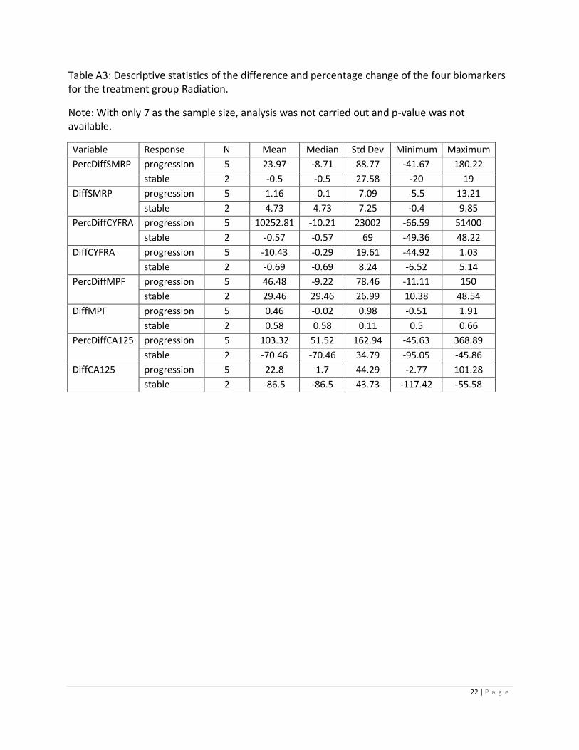
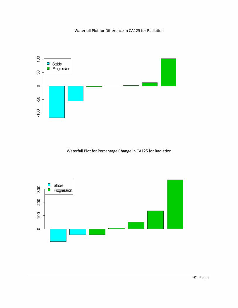
Table A3: Descriptive statistics of the difference and percentage change of the four biomarkers

for the treatment group Radiation.

Note: With only 7 as the sample size, analysis was not carried out and p-value was not

available.

Variable Response N Mean Median Std Dev Minimum Maximum

PercDiffSMRP progression 5 23.97 -8.71 88.77 -41.67 180.22

stable 2 -0.5 -0.5 27.58 -20 19

DiffSMRP progression 5 1.16 -0.1 7.09 -5.5 13.21

stable 2 4.73 4.73 7.25 -0.4 9.85

PercDiffCYFRA progression 5 10252.81 -10.21 23002 -66.59 51400

stable 2 -0.57 -0.57 69 -49.36 48.22

DiffCYFRA progression 5 -10.43 -0.29 19.61 -44.92 1.03

stable 2 -0.69 -0.69 8.24 -6.52 5.14

PercDiffMPF progression 5 46.48 -9.22 78.46 -11.11 150

stable 2 29.46 29.46 26.99 10.38 48.54

DiffMPF progression 5 0.46 -0.02 0.98 -0.51 1.91

stable 2 0.58 0.58 0.11 0.5 0.66

PercDiffCA125 progression 5 103.32 51.52 162.94 -45.63 368.89

stable 2 -70.46 -70.46 34.79 -95.05 -45.86

DiffCA125 progression 5 22.8 1.7 44.29 -2.77 101.28

stable 2 -86.5 -86.5 43.73 -117.42 -55.58

23 | P a g e

B. Figures

The deviance plot and martingale plots were used to assess the goodness-of-fit. Based on the

figures, deviance and martingale residual were bounded between [-1,1], the multi-variate

model was a good fit to the data.

Devi ance Resi dual

-2

-1

0

1

2

3

Li near Predi ct or

-2 -1 0 1 2 3 4 5 6

Figure B1: Deviance Plot

24 | P a g e

Mart i ngal e Resi dual

-3

-2

-1

0

1

Li near Predi ct or

-2 -1 0 1 2 3 4 5 6

Figure B2: Martingale residual

25 | P a g e

Figure B3 Box Plots:

26 | P a g e

27 | P a g e

28 | P a g e

29 | P a g e

30 | P a g e

31 | P a g e

32 | P a g e

33 | P a g e

34 | P a g e

35 | P a g e

36 | P a g e

Figure B4: Waterfall Plots

Waterfall Plot for Difference in SMPR for Chemotherapy -4

0-2

00

20

40

StableResponse

Progression

Waterfall Plot for Percentage Change in SMPR for Chemotherapy

05

00

15

00

25

00

35

00

StableResponse

Progression

37 | P a g e

Waterfall Plot for Difference in CYFRA for Chemotherapy -3

0-2

0-1

00

10 Stable

Response

Progression

Waterfall Plot for Percentage Change in CYFRA for Chemotherapy

01

00

00

20

00

03

00

00

StableResponse

Progression

38 | P a g e

Waterfall Plot for Difference in MPF for Chemotherapy

-5

05

10

15

StableResponse

Progression

Waterfall Plot for Percentage Change in MPF for Chemotherapy

04

00

800

12

00 Stable

Response

Progression

39 | P a g e

Waterfall Plot for Difference in CA125 for Chemotherapy

-1

00

010

02

00

30

0 Stable

Response

Progression

Waterfall Plot for Percentage Change in CA125 for Chemotherapy

05

00

01

00

00

15

00

0

StableResponse

Progression

40 | P a g e

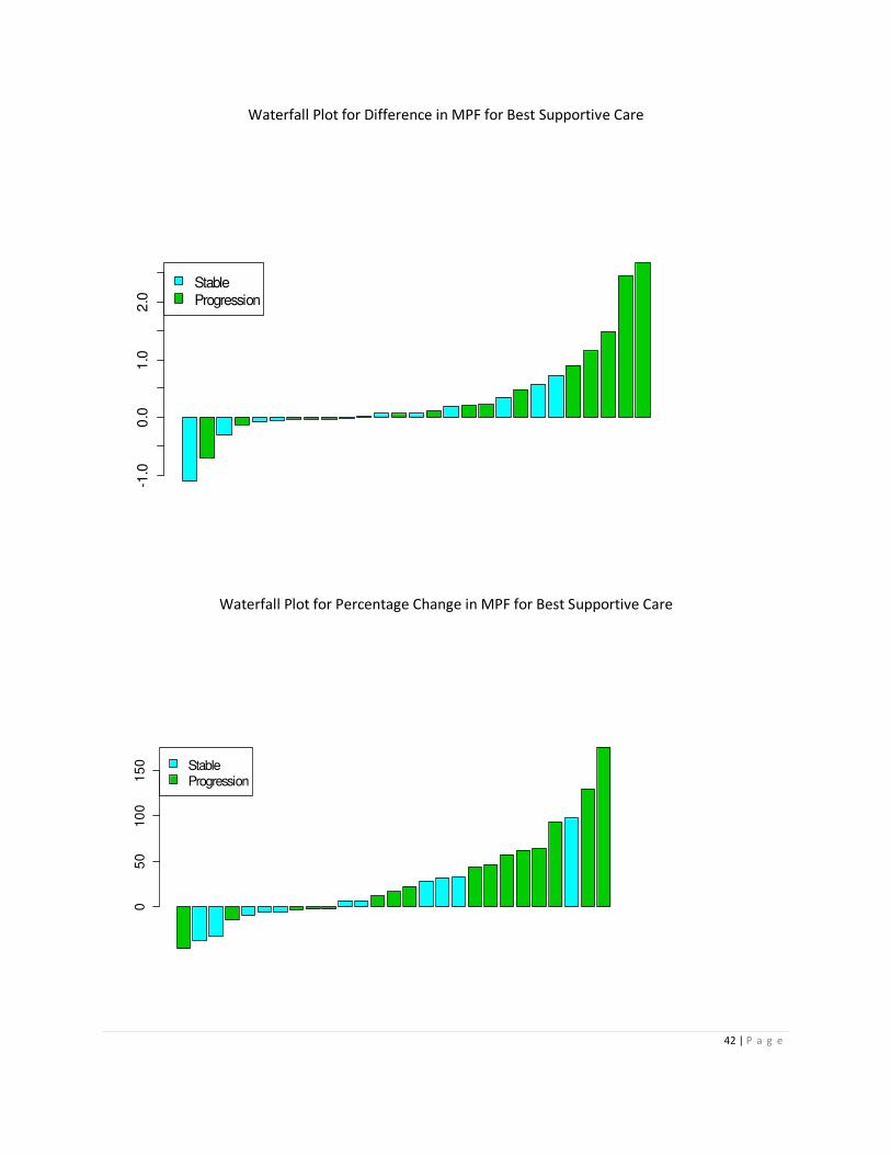
Waterfall Plot for Difference in SMRP for Best Supportive Care

-50

51

01

5

StableProgression

Waterfall Plot for Percentage Change in SMRP for Best Supportive Care

-50

05

01

00

150 Stable

Progression

41 | P a g e

Waterfall Plot for Difference in CYFRA for Best Supportive Care

020

40

60

StableProgression

Waterfall Plot for Percentage Change in CYFRA for Best Supportive Care

010

00

03

00

00

StableProgression

42 | P a g e

Waterfall Plot for Difference in MPF for Best Supportive Care

-1

.00

.01

.02

.0

Stable

Progression

Waterfall Plot for Percentage Change in MPF for Best Supportive Care

05

010

01

50 Stable

Progression

43 | P a g e

Waterfall Plot for Difference in CA125 for Best Supportive Care

-20

0-1

00

01

00

StableProgression

Waterfall Plot for Percentage Change in Ca125 for Best Supportive Care

-50

05

01

00

20

0

StableProgression

44 | P a g e

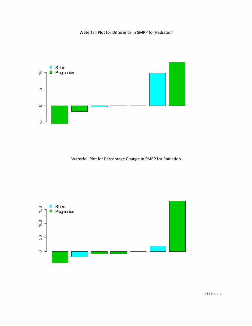
Waterfall Plot for Difference in SMRP for Radiation

-50

510

StableProgression

Waterfall Plot for Percentage Change in SMRP for Radiation

05

010

01

50 Stable

Progression

45 | P a g e

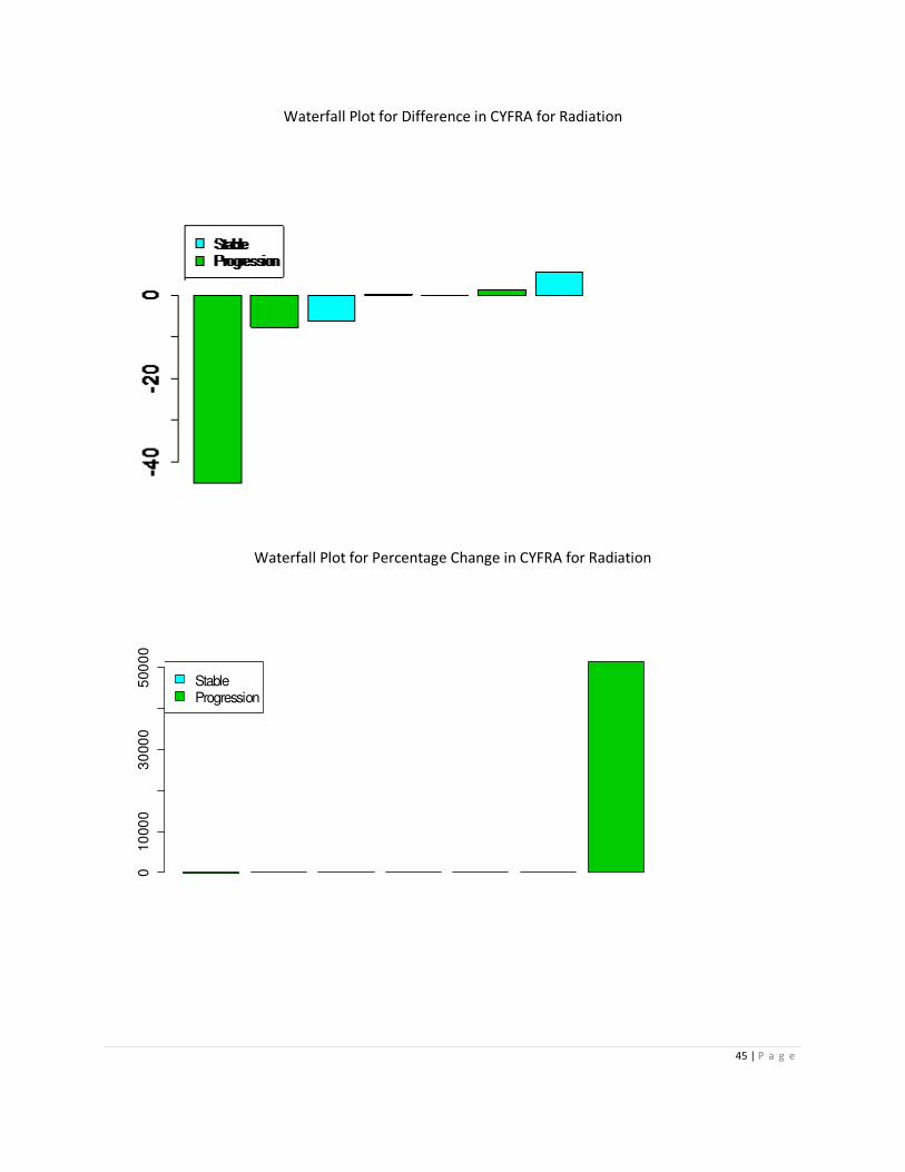
Waterfall Plot for Difference in CYFRA for Radiation

Waterfall Plot for Percentage Change in CYFRA for Radiation

010

00

03

000

05

00

00

StableProgression

46 | P a g e

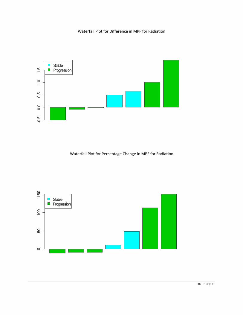
Waterfall Plot for Difference in MPF for Radiation

-0.5

0.0

0.5

1.0

1.5

StableProgression

Waterfall Plot for Percentage Change in MPF for Radiation

050

100

15

0

StableProgression

47 | P a g e

Waterfall Plot for Difference in CA125 for Radiation

-100

-50

050

100

StableProgression

Waterfall Plot for Percentage Change in CA125 for Radiation

01

00

20

03

00 Stable

Progression

48 | P a g e

SAS codes

libname m 'C:\Desktop\Geof Project';

/*Data preparation for overall survival*/

/*obtain the date of diagnosis and vital status*/

proc sort data = m.diagnosis out = dia (keep=study_no Date_of_Diagnosis); by study_no; run;

proc sort data = m.vital out = death (keep=study_no Date_of_Death If_Alive_date_last_seen);

by study_no; run;

data surv_date; merge dia death; by study_no; run;

/*calculate follow up day and assign censor info*/

data surv_date; set surv_date;

if not missing(Date_of_Death) then do;

os_cen =1;

os_day = (Date_of_Death - Date_of_Diagnosis) + 1;

end;

else if not missing(If_Alive_date_last_seen) then do;

os_cen = 0;

os_day = (If_Alive_date_last_seen - Date_of_Diagnosis) + 1;

end;

run;

*check how many patients with both pre/post and their vital;

PROC SORT DATA = m.ct_response (where=(prognosis = 'TRUE')) out=prognosis ; BY STUDY_NO

blood_1_date; RUN;

DATA PROGNOSIS; MERGE PROGNOSIS (IN=A) SURV_DATE(IN=B); BY STUDY_NO; IF A; RUN;

/*obtain baseline covariates*/

proc sort data = prognosis; by study_no; run;

proc sort data = m.pt_info out = pt_info; by study_no; run;

data prognosis; merge prognosis(in=a) pt_info(in=b); by study_no; if a; run;

/*calculate age of diagnosis*/

data prognosis; set prognosis;

age = (Date_of_Diagnosis - DOB)/365.25; run;

/*stage*/

proc sort data = m.stage out = stage; by study_no; run;

49 | P a g e

data prognosis; merge prognosis (in=a) stage (in=b); by study_no; if a; run;

/*histopath subtype*/

proc sort data = m.diagnosis out = diagnosis(keep=study_no Histopath_subtype); by study_no;

run;

data prognosis; merge prognosis (in=a) diagnosis (in=b); by study_no; if a; run;

/*surgery*/

proc sort data = m.surg out = surg(rename=(pid=study_no)); by pid; run;

data prognosis; merge prognosis (in=a) surg (in=b); by study_no; if a; run;

/*symptom*/

proc sort data = m.baseline_symptom out = baseline_symptom; by study_no; run;

data prognosis; merge prognosis (in=a) baseline_symptom (in=b); by study_no; if a; run;

/*chemo*/

proc sort data = m.chemo out = chemo (keep=study_no) nodupkey; by study_no; run;

data chemo; set chemo;

chemo = 'Yes'; run;

data prognosis; merge prognosis (in=a) chemo (in=b); by study_no; if a; run;

/*Platelet, Hemoglobin, White cell count*/

proc sort data = m.baseline_bloodtests out = baseline_bloodtests(keep=study_no WCC

Haemoglobin Platelet); by study_no; run;

data prognosis; merge prognosis (in=a) baseline_bloodtests (in=b); by study_no; if a; run;

/*grouping*/

proc format;

value ecog 0 = '0' 1 = '1/2/3';

value imig 1 = '1/2' 2 = '2' 3='3';

value smoke 0 = 'never' 1 = 'former' 2 = 'current';

run;

data prognosis; set prognosis;

if ecog = 0 then ecog_new = 0;

else if ecog > 0 then ecog_new = 1;

format ecog_new ecog.;

if imig_stage in (1,2) then imig_stage_new = 1;

else imig_stage_new = imig_stage;

format imig_stage_new imig.;

if Smoking_Status in ('Former (>1 yr)' 'Former (>1 yr) Pack years-' 'former (>1 yr)') then

smoking_status_new = 1;

else if smoking_status = 'Never' then smoking_status_new = 0;

else if smoking_status = 'Current' then smoking_status_new = 2;

50 | P a g e

format smoking_status_new smoke.;

run;

data m.prognosis; set prognosis; run;

/*Descriptive Statistics*/

ODS CSV FILE='C:\Desktop\TEMP.CSV';

proc freq data = prognosis;

table os_cen gender IMIG_Stage IMIG_Stage_new morethanonethird Histopath_subtype

Surgery Chest_Pain Weight_Loss ECOG ECOG_new Smoking_Status Smoking_Status_new

chemo WCC PLATELET HAEMOGLOBIN; run;

proc means data = prognosis n mean median std min max maxdec =2;

var os_day SMRP_result_1 CYFRA_result_1 MPF_result_1 CA125_result_1 age ; run;

proc corr data = prognosis spearman;

var SMRP_result_1 CYFRA_result_1 MPF_result_1 CA125_result_1; run;

ods csv close;

/*Survival*/

ODS CSV FILE='C:\Desktop\TEMP1.CSV';

data km; set m.prognosis;

os_yr = os_day/365.25;run;

proc lifetest data = km plots=(s);

time os_yr*os_cen(0);

run;

*continuous variables;

%macro os(var);

proc phreg data = prognosis;

model os_day*os_cen(0) = &var/risklimits; run;

%mend;

*categorical variables;

%macro os_cat(var, refvar);

proc tphreg data = prognosis;

class &var/REF=first;

model os_day*os_cen(0) = &var/risklimits; run;

%mend;

51 | P a g e

%os(SMRP_result_1);

%os(CYFRA_result_1);

%os(MPF_result_1);

%os(CA125_result_1);

%os(age);

%os_cat(gender);

%os_cat(IMIG_Stage_new);

%os_cat(morethanonethird);

%os_cat(Histopath_subtype);

%os_cat(Surgery);

%os_cat(Chest_Pain);

%os_cat(Weight_Loss);

%os_cat(ECOG_new);

%os_cat(Smoking_Status_new);

%os_cat(chemo);

%os_cat(WCC);

%os_cat(PLATELET);

%os_cat(HAEMOGLOBIN);

ods csv close;

ODS CSV FILE='C:\ Desktop\TEMP2.CSV';

*Multi-variate model;


class PLATELET Surgery /REF=first;

model os_day*os_cen(0) = PLATELET Surgery CYFRA_result_1/risklimits; run;

*interaction;


class PLATELET Surgery /REF=first;

model os_day*os_cen(0) = PLATELET Surgery CYFRA_result_1 Platelet*CYFRA_result_1

Surgery*CYFRA_result_1/risklimits; run;

*Goodness-of-fit – martingale and deviance plot;

PROC TPHREG DATA=PROGNOSIS NOPRINT;

class PLATELET Surgery/REF=first;

MODEL os_day*os_cen(0)= PLATELET Surgery CYFRA_result_1/RL ;

OUTPUT OUT=RESOUT XBETA=XB RESMART=MART RESDEV=DEV;

RUN;

SYMBOL COLOR=BLUE VALUE=DOT HEIGHT=1.0;

PROC GPLOT DATA=RESOUT;

52 | P a g e

PLOT MART*XB;

RUN;

PROC GPLOT DATA=RESOUT;

PLOT DEV*XB;

RUN; QUIT;

ods csv close;

/*Analysis on tumor response and change in biomarker value*/

*number of patients;

proc sql;

select count (distinct Study_no) from m.pt_info; quit;

*data checking;

data ct_response; set m.ct_response;

if Study_no = 116 and blood_1_date = '01MAY2010'd then blood_1_date = '01MAY2007'd;

*switch the two records;

if Study_no = 85 and blood_1_date = '06APR2010'd and blood_2_date = '10FEB2010'd then do;

blood_1_date = '10FEB2010'd;

SMRP_result_1 = 1.5;

CYFRA_result_1 = 10.76;

MPF_result_1 = 1.15;

CA125_result_1 = 2.9;

blood_2_date = '06APR2010'd;

SMRP_result_2 = 1.3;

CYFRA_result_2 = 0.36;

MPF_result_2 = 1.18;

CA125_result_2 = 8.56;

end;

run;

data ct_response; set ct_response;

if Study_no = 5 and blood_1_date = . and blood_2_date = '13NOV2009'd then tracking =

'FALSE'; run;

Data ct_response;

Set ct_response (rename =(

Study_no = PID

blood_1_date = Test1

blood_2_date = Test2

Overall_Response_of_CT = Response

SMRP_result_1 = PreSMRP

53 | P a g e

SMRP_result_2 = PostSMRP

CYFRA_result_1 = PreCYFRA

CYFRA_result_2 = PostCYFRA

MPF_result_1 = PreMPF

MPF_result_2 = PostMPF

CA125_result_1 = PreCA125

CA125_result_2 = PostCA125));

where tracking = 'TRUE';

RUN;

/*calculate difference or percentage change*/

Data ct_response_tracking; Set ct_response (drop=POST_CYFRA_NEW PRE_CYFRA_NEW);

Length response_new $20;

if response in ('Complete Response' 'Partial Response') then response_new = 'response';

else if response = 'Progressive Disease' then response_new = 'progression';

else if response = 'Stable Disease' then response_new = 'stable';

if (PreSMRP ne . and PostSMRP ne .) then do; DiffSMRP = PostSMRP - PreSMRP; PercDiffSMRP =

100*(PostSMRP - PreSMRP)/PreSMRP; end;

if (PreCYFRA ne . and PostCYFRA ne .) then do; DiffCYFRA = PostCYFRA - PreCYFRA;

PercDiffCYFRA = 100*(PostCYFRA - PreCYFRA)/PreCYFRA; end;

if (PreMPF ne . and PostMPF ne .) then do; DiffMPF = PostMPF - PreMPF; PercDiffMPF =

100*(PostMPF - PreMPF)/PreMPF; end;

if (PreCA125 ne . and PostCA125 ne .) then do; DiffCA125 = PostCA125 - PreCA125;

PercDiffCA125 = 100*(PostCA125 - PreCA125)/PreCA125; end;

Run;

/*108 RECORD WHERE TRACKING IS TRUE*/

*NOW UPDATE WHETHER IS CHEM/SURGERY OR BEST SUPPORTIVE CARE

*use the file that Sinead generate for the different category;

PROC SORT DATA = ct_response_tracking; BY PID TEST1 TEST2; RUN;

PROC SORT DATA = M.TX_RECEIVED OUT = TX_RECEIVED; BY PID TEST1 TEST2; RUN;

DATA M.ct_response_tracking; MERGE ct_response_tracking TX_RECEIVED; BY PID TEST1

TEST2; RUN;

proc corr data = M.ct_response_tracking spearman;

54 | P a g e

where chemo = 'Yes';

var preSMRP preCYFRA preMPF preCA125; run;


where bsc = 'Yes';

var preSMRP preCYFRA preMPF preCA125; run;


where chemo = 'Yes';

var postSMRP postCYFRA postMPF postCA125; run;


where bsc = 'Yes';

var postSMRP postCYFRA postMPF postCA125; run;

*descritpive statistics;

proc freq data = m.ct_response_tracking;

table (chemo bsc xrt)*response_new; run;

*boxplot;

proc format;

value resp 1 = 'Response' 2 = 'Stable' 3 = 'Progression'; run;

data boxplotdata; set m.ct_response_tracking;

if response_new = 'progression' then response_new_num = 3;

if response_new = 'stable' then response_new_num = 2;

if response_new = 'response' then response_new_num = 1;

format response_new_num resp.;

run;

proc sort data = boxplotdata; by response_new_num; run;

goptions reset = all ftext=simplex;

options pageno=1 center;

options orientation=portrait nodate nonumber;

ods rtf file = 'C:\ Desktop\graph.rtf';

ods graphics on;

%macro plot_box(title_name,categ,var1);

axis1 label=("");

axis2 label=("") order=(1 to 3 by 1) ;

title "Box Plot for &title_name";

proc boxplot data= boxplotdata;

55 | P a g e

where &categ = 'Yes';

plot &var1*response_new_num/vaxis = axis1 haxis=axis2;

run;

%mend;

%plot_box(Percentage Change in SMRP for Chemo, chemo, PercDiffSMRP);

%plot_box(Difference in SMRP for Chemo, chemo, DiffSMRP);

%plot_box(Percentage Change in CYFRA for Chemo, chemo, PercDiffCYFRA);

%plot_box(Difference in CYFRA for Chemo, chemo, DiffCYFRA);

%plot_box(Percentage Change in MPF for Chemo, chemo, PercDiffMPF);

%plot_box(Difference in MPF for Chemo, chemo, DiffMPF);

%plot_box(Percentage Change in CA125 for Chemo, chemo, PercDiffCA125);

%plot_box(Difference in CA125 for Chemo, chemo, DiffCA125);

%plot_box(Percentage Change in SMRP for Best Supportive Care, BSC, PercDiffSMRP);

%plot_box(Difference in SMRP for Best Supportive Care, BSC, DiffSMRP);

%plot_box(Percentage Change in CYFRA for Best Supportive Care, BSC, PercDiffCYFRA);

%plot_box(Difference in CYFRA for Best Supportive Care, BSC, DiffCYFRA);

%plot_box(Percentage Change in MPF for Best Supportive Care, BSC, PercDiffMPF);

%plot_box(Difference in MPF for Best Supportive Care, BSC, DiffMPF);

%plot_box(Percentage Change in CA125 for Best Supportive Care, BSC, PercDiffCA125);

%plot_box(Difference in CA125 for Best Supportive Care, BSC, DiffCA125);

%plot_box(Percentage Change in SMRP for XRT, XRT, PercDiffXRT);

%plot_box(Difference in SMRP for XRT, XRT, DiffXRT);

%plot_box(Percentage Change in CYFRA for XRT, XRT, PercDiffCYFRA);

%plot_box(Difference in CYFRA for XRT, XRT, DiffCYFRA);

%plot_box(Percentage Change in MPF for XRT, XRT, PercDiffMPF);

%plot_box(Difference in MPF for XRT, XRT, DiffMPF);

%plot_box(Percentage Change in CA125 for XRT, XRT, PercDiffCA125);

%plot_box(Difference in CA125 for XRT, XRT, DiffCA125);

ods graphics off;

ods rtf close;

*Krustal-Wallis or Mann-Whiteney;


Proc Npar1way data = m.ct_response_tracking Wilcoxon;

Class response_new;

Var PercDiffSMRP DiffSMRP PercDiffCYFRA DiffCYFRA PercDiffMPF DiffMPF PercDiffCA125

DiffCA125;

Where Chemo = "Yes";

Run;

56 | P a g e


Class response_new;


DiffCA125;

Where BSC = "Yes";

Run;


Class response_new;


DiffCA125;

Where XRT = "Yes";

Run;

ods csv close;

*descriptive statistics;


proc means data = m.ct_response_tracking n mean median std min max maxdec = 2;

Class response_new;


DiffCA125;

Where Chemo = "Yes";

run;


Class response_new;


DiffCA125;

Where BSC = "Yes";

run;


Class response_new;


DiffCA125;

Where XRT = "Yes";

run;

ods csv close;

57 | P a g e

R Code was used to generate waterfall plots. A sample of the code used to generate the graphs

for the chemotherapy group and biomarker SMRP is shown below. Codes for Best Supportive

Care and Radiation are very similar and thus they are not provided here.

#Chemo

x<- read.csv("C:\\Documents and Settings\\XPMUser\\Desktop\\clean.csv", sep=',', dec='.',

na.strings='')

x$Response2 <- as.numeric(x$Response)+2

x2<-x[x$Chemo=='Yes',]

x2<-x2[order(x2$DiffSMRP),]

plot(x2$DiffSMRP, col=x2$Response, type='h', lwd=5, ylim=c(-100,4000), xlab='', ylab='',

cex.axis=1.5, cex.lab=1.5)

abline(h=0)

temp<-cbind(x2$DiffSMRP,x2$Response)

barplot(x2$DiffSMRP, col=as.numeric(x2$Response)+2)

legend("topleft", legend=c("Stable","Response","Progression"), col=c(5,4,3), fill=c(5,4,3))

x2<-x2[order(x2$PercDiffSMRP),]

plot(x2$PercDiffSMRP, col=x2$Response, type='h', lwd=5, ylim=c(-100,4000), xlab='', ylab='',

cex.axis=1.5, cex.lab=1.5)

abline(h=0)

temp<-cbind(x2$PercDiffSMRP,x2$Response)

barplot(x2$PercDiffSMRP, col=as.numeric(x2$Response)+2)

legend("topleft", legend=c("Stable","Response","Progression"), col=c(5,4,3), fill=c(5,4,3))