series: ecmwf - esa contract report...... esa contract report a full list of ... are from the...
TRANSCRIPT


Series: ECMWF - ESA Contract Report A full list of ECMWF Publications can be found on our web site under: http://www.ecmwf.int/publications/ © Copyright 2006 European Centre for Medium Range Weather Forecasts Shinfield Park, Reading, RG2 9AX, England
Literary and scientific copyrights belong to ECMWF and are reserved in all countries. This publication is not to be reprinted or translated in whole or in part without the written permission of the Director. Appropriate non-commercial use will normally be granted under the condition that reference is made to ECMWF.
The information within this publication is given in good faith and considered to be true, but ECMWF accepts no liability for error, omission and for loss or damage arising from its use.

Contract Report to the European Space Agency
The technical support for global validation of ERS Wind and Wave Products at ECMWF
(April 2004 - June 2006)
Authors: Saleh Abdalla and Hans Hersbach
Final report for ESA contract 18212/04/I-OL
European Centre for Medium-Range Weather Forecasts
Shinfield Park, Reading, Berkshire, UK
August 2006

ESA report on ERS Wind and Wave Products
Abstract
Contracted by ESA/ESRIN, ECMWF is involved in the global validation and long-term performance mon-itoring of the wind and wave Fast Delivery products that are retrieved from the Radar Altimeter (RA), theSynthetic Aperture Radar (SAR) and the Active Microwave Instrument (AMI), on-board the ERS spacecraft.Their geophysical content is compared with corresponding parameters from the ECMWF atmospheric andwave model as well as in-situ observations (when possible). Also, tests on internal data consistency areperformed.
The project (18212/04/I-OL), which ran from 1 April 2004 to 30 June 2006, is the continuation of previ-ous contracts initiated with ESA/ESRIN and ESTEC. This note presents the final report on the activitiesperformed within the scope of this contract.
An ERS-2 on-board failure in January 2001 degraded attitude control. It had a negative, though acceptable,effect on the quality of the RA and SAR related products; however, a detrimental effect on AMI scatterom-eter winds. The problems in attitude control were gradually resolved, and since August 2003 the quality ofall products is nominal. After 21 June 2003, ERS-2 lost its global coverage permanently due to the failureof both on-board tape recorders. However, the remaining coverage (North Atlantic and western coasts ofNorth America And at a later stage the Southern Ocean and the coasts of East Asia) provides valuable datafor assimilation in atmospheric models. Focus of this report will be on that period.
Furthermore, an overview evaluation of the wind and wave products from the entire ERS mission is carriedout. The products involved are the fast delivery AMI scatterometer wind and SAR wave mode spectra andthe off-line ocean product (OPR) wind and wave data from both ERS-1 and ERS-2 missions.
1 Introduction
The ERS mission is a great opportunity for the meteorological and ocean-wave communities. The wind andwave products from ERS-1/2 provide an invaluable data set. They form some kind of benchmarks against whichmodel products can be validated. In addition, they are assimilated in the models to improve the predictions. Onthe other hand, consistent model products, especially first-guess products, can be used to validate and monitorthe performance of the satellite products.
The European Centre for Medium-Range Weather Forecasts (ECMWF) has been collaborating with the Euro-pean Space Agency (ESA) since the beginning of the ERS-1 mission in performing the global validation andlong-term performance monitoring of the wind and wave products. These products are retrieved from threeinstruments, defining three Fast Delivery (FD) products that are received at ECMWF in BUFR format. Signif-icant wave height and surface wind speed (URA product) are obtained from the Radar Altimeter (RA). Oceanimage spectra (UWA product) are from the Synthetic Aperture Radar (SAR). Surface wind speed and direction(UWI product), finally, are retrieved from the Active Microwave Instrument (AMI) scatterometer. In-housedeveloped monitoring tools are used for the comparison of these products with corresponding parameters fromthe ECMWF atmospheric (IFS) and wave (ECWAM) models (IFS Documentation, 2004). Whenever possible,these tools include a comparison with in-situ measurements. In addition, tests are performed on the internalconsistency of the underlying observed quantities measured by the three instruments.
This support has been carried out within the framework of several consecutive contracts with ESA. The cur-rent contract (18212/04/I-OL), which is supervised by the European Space Research Institute (ESRIN), ranfrom 1 April 2004 to 30 June 2006. Findings from the monitoring activities described above are summarizedin monthly or cyclic (depending on the product) data quality and validation reports. These reports are sentregularly to ESRIN. Besides giving an overview on instrument performance and scientific interpretation, these
ESA report 1
ESA report on ERS Wind and Wave Products
reports also include recommendations to ESA for refinements of calibrations, further algorithm developmentand model tuning. Such recommendations are based on a long-term analysis of the relevant parameters.
In addition to these monitoring activities, dedicated studies on data quality and related scientific research havebeen carried out. These embrace, among others, collocation studies, algorithm development and the incorpo-ration of ERS wind and wave data in the operational ECMWF assimilation system. As a result, ERS altimeterwave heights have been assimilated in the ECMWF wave model since 15 August 1993 (Janssen et al. 1997).It was replaced by ENVISAT Radar Altimeter-2 (RA-2) on 22 October 2003. Scatterometer winds were intro-duced in the atmospheric variational assimilation system on 30 January 1996 (for a description of its impact,see Isaksen and Janssen 2004). It was re-introduced on 8 March 2004 (Hersbach et al. , 2004a), after the sus-pension in January 2001. The assimilation of SAR wave mode spectra in the ECMWF wave model, on theother hand, was realised on 13 January 2003. ERS-2 SAR assimilation was replaced by ENVISAT AdvancedSynthetic Aperture Radar (ASAR) Level 1b wave mode spectra on 1 February 2006.
This document presents the final report of the present contract. It provides a focus on the performance of thewind and wave products over a period of about three years.
Since the ERS mission is approaching the end of its lifetime, it is thought opportune to make a review of thequality of the various products from both ERS-1 and ERS-2 satellites. Those products are the fast delivery (FD)scatterometer wind (UWI) product, FD SAR Wave Mode (UWA) product and both FD (URA) and the off-lineOPR (Ocean Product) altimeter wind and wave products.
In Section 2, the performance of altimeter FD URA data in the North Atlantic will be considered. Section 3presents the global performance of the altimeter OPR product for the whole lifetime of the ERS mission. Anoverview of the performance of the SAR significant wave height, both globally and in the North Atlantic, willbe presented in Section 4, and of UWI wind data in Section 5. In Section 6, conclusions are formulated, andthe report ends with a list of ECMWF model changes since November 2000.
2 ESA report

ESA report on ERS Wind and Wave Products
Acronyms
AMI Active Microwave InstrumentASPS Advanced Scatterometer Processing SystemAOCS Attitude and Orbit Control SystemASAR Advanced Synthetic Aperture RadarASCAT Advanced SCATterometerASCII American Standard Code for Information InterchangeBUFR Binary Universal Form for the Representation of meteorological dataCERSAT French ERS Processing and Archiving Facility (Centre ERS d’Archivage et de Traitement)CMEDS Canadian Marine Environmental Data ServiceCMOD C-band Geophysical MODel functionEBM Extra Back-up ModeECMWF European Centre for Medium-range Weather ForecastsECWAM ECMWF WAve Model (an enhanced version of WAM model)ENVISAT ENVIronmental SATelliteERA-40 ECMWF 40-Year ReanalysisERS European Remote sensing SatelliteESA European Space AgencyESACA ERS Scatterometer Attitude Corrected AlgorithmESTEC European Space research and TEchnology CentreESRIN European Space Research INstituteFD Fast Delivery productFEEDBACK data to which information on usage in the ECMWF assimilation system has been addedFG ECMWF First Guess with a time resolution of 3 hoursFGAT First Guess at Appropriate TimeGMF scatterometer Geophysical Model FunctionGTS Global Telecommunication SystemHRES High RESolutionIDL Interactive Data LanguageIFREMER French Research Institute for Exploitation of the Sea
(Institut francais de recherche pour l’exploitation de la mer)IFS Integrated Forecast SystemJPL Jet Propulsion LaboratoryKNMI Koninklijk Nederlands Meteorologisch InstituutLRDPF Low Rate Data Processing FacilityLBR Low Bit RateMPI Max-Planck-Institut for meteorology, HamburgNESDIS National Environmental Satellite Data and Information ServiceNDBC U.S. National Data Buoy CenterNH Northern HemisphereNRES Nominal RESolutionNRT Near-Real TimeNSCAT NASA (National Aeronautics and Space Agency) ScatterometterOPR (ERS Radar Altimeter) Ocean PRoduct
ESA report 3

ESA report on ERS Wind and Wave Products
QC Quality ControlQSCAT QuikSCAT (Quick Scatterometer)RA Radar AltimeterRA-2 (ENVISAT) Radar Altimeter-2RMSE Root-Mean Square ErrorSAR Synthetic Aperture RadarSH Southern HemisphereSI Scatter IndexSTDV STandard DeViation (of the Difference)SWH Significant Wave HeightTAO Tropical Atmosphere Ocean projectUKMO UK Met OfficeURA User FD Radar Altimeter productUTC Coordinated Universal TimeUWA User FD SAR WAve productUWI User FD scatterometer WInd productWAM third-generation ocean-WAve ModelWMO World Meteorological OrganizationZGM Zero-Gyro Mode
4 ESA report

ESA report on ERS Wind and Wave Products
2 The Radar Altimeter URA Product
Each URA (User fast delivery Radar Altimeter) product is sampled at 7 km along the satellite ground track. Firstthe altimeter data stream is divided into sequences of 30 individual neighbouring observations. Erroneous andsuspicious individual observations are removed and the remaining data in each sequence are averaged to forma representative super-observation, provided that the sequence has at least 20 ”good” individual observations.Then, further monitoring is performed with respect to these super-observations, which, for this purpose arecollocated with ECMWF model parameters and buoy data. Focus is on URA backscatter, URA wind speed andURA significant wave height.
2.1 Data Coverage after June 2003
The loss of the global coverage due to the failure of the on-board low-bit rate tape recorders in June 2003reduced the number of observations received at ECMWF to about 13% of the full coverage data volume as canbe seen in Figure 1 which shows the daily rate of total number of the altimeter super-observations processedat ECMWF. Assessment of the long-term quality of the product after the loss of the global coverage can notbe done by comparing it with statistics when there was full coverage. For practical reasons it is not easy to re-process the product over a rather long period for the exact area under current coverage. Instead, readily availablelong-term statistics for the closest region is considered for comparison. The region covering the extra-tropicalNorthern Atlantic (north of latitude 20
�
N) is used as a common area with almost complete coverage before andafter the loss of the global coverage. The 7-day running average of daily number of altimeter super-observationsin the North Atlantic since the beginning of year 2000 is shown in Figure 2. It is clear that the current coveragein the North Atlantic is slightly lower than the usual coverage. The missing coverage is towards the southernedge of the region as can be seen in Figure 3. For the URA product, we will focus our attention on the qualityof the altimeter products for the current coverage or specifically in the North Atlantic.
2.2 Monitoring of URA Significant Wave Height in the North Atlantic
As usual, URA significant wave heights (SWH) are rather stable and of good quality, apart from the overes-timation of small SWH values. Figure 4 shows the time history of the daily bias between the altimeter andthe ECMWF operational model wave heights in the North Atlantic since the beginning of year 2000. Afterexcluding the apparent anomalous altimeter behaviour during March-April 2000 and February 2001 one candistinguish a seasonal cycle of bias in Figure 4 with a minimum value taking place around April-May and amaximum value occurring around October-November before the loss of the global coverage. This seasonalcycle became stronger after the loss of the global coverage with the minimum and maximum values shiftedearlier by about one month. Although it is difficult to pinpoint the reason for the stronger cycle, recent modelchanges like the unresolved bathymetry treatment introduced on 9 March 2004 and the change of wave modeldissipation introduced on 5 April 2005 are possible candidates. Another possible reason could be related to theuncovered part towards the southern edge of the area (see Figure 3) which shows less variability than the higherlatitudes. Figure 4 displays a clear general trend of reduced bias over the years as well. This is mainly due tothe model improvements. Recently, the bias seems to fluctuate around the zero value. Apart from that, the biasbetween the altimeter and the model wave heights did not suffer any abrupt changes after the loss of the globalcoverage.
Figure 5 shows the time history of the daily scatter index (SI) of the altimeter significant wave height withrespect to the ECMWF wave model (ECWAM) in the North Atlantic since the beginning of year 2000. Boththe seasonal variation (maximum during July-August and minimum during December-January) and the general
ESA report 5

ESA report on ERS Wind and Wave Products
01-01-00 31-12-00 01-01-02 01-01-03 01-01-04 31-12-04 01-01-06 01-01-070
200
400
600
800
1000
1200
1400
1600
1800
Num
ber
of
RA
Sup
er-O
bser
vatio
ns p
er D
ay
Figure 1: Time history of the total number of ERS-2 altimeter super-observations processed at ECMWF per day since 1January 2000. Date of loss of global coverage is represented by a red thick vertical line.
01-01-00 31-12-00 01-01-02 01-01-03 01-01-04 31-12-04 01-01-06 01-01-0750
100
150
200
250
Num
ber
of
RA
Sup
er-O
bser
vatio
ns p
er D
ay
Figure 2: Time history of the 7-day running average of daily number of altimeter super-observations in the North Atlanticsince 1 January 2000. Date of loss of global coverage is represented by a red thick vertical line.
6 ESA report

ESA report on ERS Wind and Wave Products
Figure 3: Typical recent ERS-2 radar altimeter monthly coverage (June 2006).
01-01-00 31-12-00 01-01-02 01-01-03 01-01-04 31-12-04 01-01-06 01-01-07-0.2
-0.1
0.0
0.1
0.2
0.3
ER
S-2
RA
SW
H B
ias
= E
RS
- W
AM
(m
)
Figure 4: Time history of the 7-day running average of daily bias of altimeter significant wave height with respect to wavemodel in the North Atlantic since 1 January 2000. Date of loss of global coverage is represented by a red thick verticalline.
ESA report 7

ESA report on ERS Wind and Wave Products
01-01-00 31-12-00 01-01-02 01-01-03 01-01-04 31-12-04 01-01-06 01-01-070.05
0.10
0.15
0.20
0.25E
RS-
2 R
A S
WH
Sca
tter
Inde
x w
.r.t.
WA
M
7-day running average365-day running average
Figure 5: Time history of the 7-day running average of daily scatter index of altimeter significant wave height withrespect to wave model in the North Atlantic since 1 January 2000. The thick black line shows the SI trend (365-dayrunning average). Date of loss of global coverage is represented by a red thick vertical line.
trend of the reduction in SI (the 365-day running average) can be seen. Again the seasonal variation seems tobe stronger after the loss of global coverage. The higher SI values during July and August 2004 are due to atechnical problem that prevented the ENVISAT RA-2 SWH product from being assimilated in the wave model.
In summary, it is possible to say that the altimeter significant wave height product is as good as it used to be.Other statistics (not shown) deliver the same message. It is worth mentioning that the ERS-2 altimeter waveheight product was assimilated in the ECMWF wave model until it was replaced by the corresponding productfrom ENVISAT on 21 October 2003.
2.3 Monitoring of URA Surface Wind Speed in the North Atlantic
Before the loss of the global coverage, URA wind speed observations were not as good as the wave heights.They suffered several periods of degraded quality, especially after the start of the problems with the on-boardgyros early 2000 as will be described later in Section 3.4. The ”sun blinding effect” is responsible for most ofthe degradation in the Southern Hemisphere (SH) during the period between mid-January to early March eachyear since year 2000.
Figure 6 shows the time history of the daily bias of URA surface wind speed with respect to the ECMWFoperational atmospheric model in the North Atlantic since 1 January 2000. The wind speed bias in the NorthAtlantic follows a seasonal cycle with positive bias (maximum) in the Northern Hemispheric (NH) winter andnegative (minimum) in the NH summer can be clearly seen. Since early 2001, this seasonal cycle startedto be symmetric around the zero line. This can be attributed to the ECMWF high-resolution model T511implemented on 20 November 2000. The same behaviour continued after the loss of the global coverage.On the other hand, Figure 7 shows the time history of the daily SI of surface wind speed with respect to the
8 ESA report

ESA report on ERS Wind and Wave Products
01-01-00 31-12-00 01-01-02 01-01-03 01-01-04 31-12-04 01-01-06 01-01-07-1.5
-1.0
-0.5
0.0
0.5
1.0
1.5
ER
S-2
RA
Win
d Sp
eed
Bia
s =
ER
S -
Mod
el
(
m/s
)
Figure 6: Time history of the 7-day running average of daily bias of altimeter surface wind speed with respect to theECMWF atmospheric model in the North Atlantic since 1 January 2000. Date of loss of global coverage is representedby a red thick vertical line.
ECMWF operational atmospheric model in the North Atlantic since 1 January 2000. The SI follows a seasonalcycle with low values occurring during the NH winter and vice versa in summer. The exception to this cycleis the period from early January to early March each year since 2001. This may be due the residual effect ofthe ”sun blinding effect”. Continuous improvements of the ECMWF operational atmospheric model result inlower wind speed scatter index values between this model and the altimeter. A drop in SI early 2002 can beclearly recognised. This coincides with a model change including the assimilation of QuikSCAT wind speeds.The usual trend of the SI reduction continued after the reduction of ERS-2 coverage. The only exception is therelatively higher scatter index during January and February 2004.
2.4 Monitoring of URA Altimeter Backscatter
Altimeter backscatter is the raw observation that is translated into surface wind speed. Figure 8 displays thelong-term monthly global mean backscatter coefficient values since December 1996. Before the loss of theglobal coverage, the monthly mean value used to be around 11.0 dB. However, the mean values used to increaseto more than 11.4 dB for the month of July in years 1997 to 1999. Those peaks disappeared in year 2000 andlater. Instead, the mean backscatter coefficient started to be rather low in the month of February (or March)each year from 2000. This is a direct result from the sun blinding effect.
After the loss of the global coverage, the monthly mean started to have a strong seasonal cycle varies between10.4 and 12.2 dB. This cycle has a peak during the NH summer (July-August) and a trough during winter(December-January). This is an expected behaviour in the NH. After the extension of the ERS-2 coverage byincluding more ground stations especially in the SH, the amplitude of the seasonal cycle of mean backscattercoefficient started to get smaller. The impact of including McMurdo and Hobart ground stations can not bemissed in Figure 8.
ESA report 9

ESA report on ERS Wind and Wave Products
01-01-00 31-12-00 01-01-02 01-01-03 01-01-04 31-12-04 01-01-06 01-01-070.10
0.15
0.20
0.25
0.30
ER
S-2
RA
Win
d Sp
eed
Sca
tter
Inde
x w
.r.t.
Mod
el
Figure 7: Time history of the 7-day running average of daily scatter index of altimeter surface wind speed with respect tothe ECMWF atmospheric model in the North Atlantic since 1 January 2000. Date of loss of global coverage is representedby a red thick vertical line.
Dec
96
Jun
97
Dec
97
Jun
98
Dec
98
Jun
99
Dec
99
Jun
00
Dec
00
Jun
01
Dec
01
Jun
02
Dec
02
Jun
03
Dec
03
Jun
04
Dec
04
Jun
05
Dec
05
Jun
06
10.4
10.6
10.8
11.0
11.2
11.4
11.6
11.8
12.0
12.2
12.4
Bac
ksca
tter,
σo
(dB
)
Reduced Coverage
McMurdo
Hob
art
Figure 8: Time history of the monthly global mean of ERS-2 altimeter backscatter coefficient after QC since December1996.
10 ESA report

ESA report on ERS Wind and Wave Products
3 The Radar Altimeter OPR Product
3.1 Introduction
The ERS missions started with the launch of ERS-1 (the first sun-synchronous polar-orbiting mission of ESA)on 17 July 1991. It was followed by ERS-2 which was launched on 21 April 1995. The Radar Altimeter (RA)and the Active Microwave Instrument (AMI) which consists of two separate radars; namely: the Synthetic-Aperture Radar (SAR) and the Scatterometer, are the instruments which are able to provide wind and wave dataon-board both satellites.
According to ESA (2005), the launch and early orbit phase (LEOP) of ERS-1 began with the launch andended with the satellite achieving nominal attitude and orbit. The duration of this initial phase was less thantwo weeks. A 3-day repeat cycle was adopted to provide frequent revisits to a number of dedicated sitesfor calibration purposes. The remaining effective life of the ERS-1 mission is sub-divided into the followingphases:
� Phase A - Commissioning Phase: 3-day repeat cycle. Lasted 138 days (from 25 July to 10 December1991). Mainly to perform engineering calibration and geophysical validation.
� Phase B - First Ice Phase: 3-day repeat cycle. Lasted 93 days (from 28 December 1991 to 31 March1992). Optimised for the specific requirements of Arctic ice experiments.
� Phase R - Experimental Roll Tilt Mode Campaign: 35-day repeat cycle. Lasted 12 days (from 2 to 14April 1992). The satellite body was rotated by 9.5 degrees allowing operation of the SAR imaging modeat an incidence angle of 35 degrees. Performance of the RA Altimeter is slightly degraded because of thegeocentric pointing instead of the local normal pointing.
� Phase C - Multi-Disciplinary Phase: 35-day repeat cycle. Lasted 20 months (14 April 1992 to 23December 1993). Mean sea surface determination, ocean variability studies and surface mappings areamong various uses during this phase.
� Phase D - Second Ice Phase: 3-day repeat cycle similar to the First Ice Phase (Phase B). Lasted 108days (from 23 December 1993 to 10 April 1994).
� Phase E - Geodetic Phase: 168-day repeat cycle. Lasted about 5 months (from 10 April 1994 to 28September 1994). Enables high-density measurements to improve the determination of the geode usingRA.
� Phase F - Shifted Geodetic Phase: 168-day repeat cycle similar to the Geodetic Phase (Phase E) butwith an 8 km spatial shift. Lasted about 6 months (from 28 September 1994 to 21 March 1995).
� Phase G - Second Multi-Disciplinary Phase: 35-day repeat cycle similar to the first Multi-DisciplinaryPhase (Phase C). Lasted about 14 months (from 21 March 1995 to 2 June 1996). Tandem mission withERS-2 (from 17 August 1995 to 2 June 1996) was within this phase.
Phase G concluded the nominal ERS-1 mission. ERS-1 stayed in this configuration while serving as a back upfor ERS-2. ERS-1 finally retired on 10 March 2000 after a failure in its on-board attitude control system.
On the other hand, ERS-2 had only two phases of operations both with the same orbital configuration of 35-dayrepeat cycle:
ESA report 11
ESA report on ERS Wind and Wave Products
� Phase A - Commissioning Phase: Lasted from 2 May 1995 to 17 August 1995. Mainly to performengineering calibration and geophysical validation.
� Phase B - Routine Phase: Started on 17 August 1995 and still going on. Similar to ERS-1 Phases C andG. This phase started with the tandem mission from 17 August 1995 to 2 June 1996.
ERS-2 was unfortunate to start loosing its gyroscopes in early 2000. This lead to the implementation of theAttitude and Orbit Control System (AOCS) mono-gyro attitude software early February 2000 (c.f. Femeniasand Martini, 2000). Further loss of gyroscopes on 17 January 2001, which left a single working gyroscope,forced the piloting of the spacecraft without any gyroscopes in the Extra Back-up Mode (EBM). This led todegradation of some ERS-2 products. The implementation of the zero-gyro mode (ZGM) was introduced inJune 2001 to assist the piloting of the spacecraft without any need for the frequent use of the only availablegyroscope.
Finally, the permanent failure of the ERS-2 low bit rate (LBR) tape recorders on 21 June 2003 prevented thecontinuation of the ERS-2 global coverage. ERS-2 LBR data coverage is limited within the vicinity of theground stations. The recent coverage map is shown in Figure 3.
3.2 Data Sources and Collocations
ERS altimeter OPR data products were obtained from the French ERS Processing and Archiving Facility (CER-SAT) of the French Research Institute for Exploitation of the Sea (IFREMER). The data were converted intoBUFR format. The same operational pre-processing and quality control procedures (c.f. Abdalla and Hersbach,2004) were applied before the use of the data. The only exception is that the number of 1-Hz observations av-eraged to produce one super-observation was selected to be 11 (rather than the value of 30 used operationallyfor ERS-2).
As both operational atmospheric and wave models at ECMWF are changing frequently, the operational ECMWFdata archive does not represent a consistent data set to be used for the evaluation of the ERS products. The qual-ity of both wind and wave fields are improving with time. Since we are after a long-term evaluation of ERSproducts, a more consistent data set (free of other changes) is needed. Therefore, it was found appropriate to usethe ECMWF 40-Year Reanalysis (ERA-40) wind fields for the validation. ERA-40 fields were produced usingthe same atmospheric model for the entire period of the reanalysis from September 1957 to August 2002. Themodel used in the reanalysis has a spectral resolution of T159 (c.f. Uppala et al., 2005) which corresponds toabout 125 km. Although this is much coarser than the operational resolution during the last few years, ERA-40resolution is much higher than the operational resolutions at earlier times. Furthermore, ERA-40 represents arather consistent data set as far as the model is concerned. The amount and quality of the observations assimi-lated in ERA-40 varied by time during the ERA-40 period. This, of course, has some (hopefully minor) impacton the consistency of ERA-40 products. However, in the absence of another alternative, one can make use ofthis data set.
The wave model used in ERA-40 was of rather coarser resolution (1.5 degree which is about 156 km). Althoughthis may not be a major concern in the open ocean, it has a definite detrimental impact on wave fields in theinner seas and near the coasts. Therefore, we decided not to use ERA-40 wave fields for the evaluation of ERSOPR wave products. Instead a long term stand-alone wave model hindcast run (without any data assimilation)was used. The model used for this run is the latest version of the ECMWF wave model (ECWAM) whichincludes several enhancements, both physics and numerics, over the standard WAM model (c.f. Janssen, 2004,Janssen et al., 2005 and Bidlot et al., 2006). The model resolution is 0.5 degrees (about 55 km). ERA-40 windfields were used to force the model.
12 ESA report
ESA report on ERS Wind and Wave Products
1991
-01-
01
1992
-01-
01
1992
-12-
31
1994
-01-
01
1995
-01-
01
1996
-01-
01
1996
-12-
31
10000
15000
20000
25000
30000
Num
ber
of S
uper
-obs
. / w
eek
Phase A
Phase B
Phase C Phase D
Phase E
Phase F
Phase G
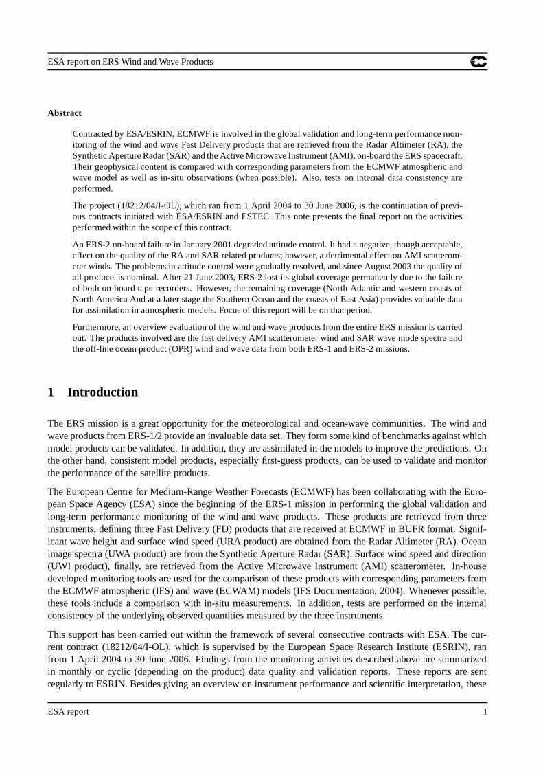
Figure 9: Time history of the 5-week running average of weekly number of ERS-1 altimeter super-observations during theeffective lifetime of ERS-1 (August 1991 to May 1996). Various ERS-1 phases are displayed.
The ERA-40 data set covers the period until 31 August 2002. After that date, operational wind fields were usedfor ERS-2 wind speed products. The same wind fields were used to force the wave model beyond ERA-40period. It is important to note that the operational wind fields are of much better quality than ERA-40 due tothe recent model enhancements and to the higher resolution. Naturally one should expect better wave fields asa result of using such wind fields for the hindcast run.
The radar altimeter super-observations were collocated with the corresponding model counterparts. Each weekworth of collocations are used to compute various statistics. The time histories of those statistics are examinedto draw conclusions related to the altimeter wind and wave products. To concentrate on long-term changes itwas necessary to filter out the short term variability (noise) of those plots by using 5-weekly running averages.
3.3 ERS-1 Altimeter OPR Product
Figure 9 shows the time history of the weekly number of super-observations of ERS-1 altimeter OPR productsduring the effective lifetime of ERS-1 (August 1991 to May 1996). Note that the number of 1-Hz observationsaveraged to form each super-observation is 11. This is the reason for the higher number of super-observationscompared to the operational plots of URA product (e.g. ERS-2 URA plot of Figure 1).
Figure 10 shows the time history of the weekly bias of ERS-1 altimeter significant wave height with respectto the ECWAM model hindcast (using ERA-40 reanalysis wind fields) during the effective lifetime of ERS-1. Both (absolute) bias and bias relative to the model mean (relative bias) are shown. It is clear that ERS-1OPR SWH is in general lower than the model by about 18 cm (about 7%). The seasonal cycle of the biascan not be missed. Normalising with the mean model wave height does not totally eliminate this seasonalcycle. The underestimation of ERS-1 SWH with respect to the model varies between about 12 cm (during theNH summer) and about 24 cm (in NH winter). This corresponds to about 5% and 11%, respectively. It isworthwhile mentioning that during the first two months of the ERS-1 mission (August-September 1991), the
ESA report 13

ESA report on ERS Wind and Wave Products
1991
-01-
01
1992
-01-
01
1992
-12-
31
1994
-01-
01
1995
-01-
01
1996
-01-
01
1996
-12-
31
-0.40
-0.30
-0.20
-0.10
0.00
0.10
Bia
s
(m
)
or
R
elat
ive
Bia
s
Relative BiasBias
Phase A
Phase B
Phase C Phase D
Phase E
Phase F
Phase G
Figure 10: Time history of the 5-week running average of weekly global bias and relative bias (i.e. the bias normalised bythe model mean) of ERS-1 altimeter significant wave height with respect to the ECWAM model hindcast (using ECMWFERA-40 reanalysis wind fields) during the effective lifetime of ERS-1 (August 1991 to May 1996). Various ERS-1 phasesare displayed.
SWH bias was the smallest ever during the entire mission. It seems that the various ERS-1 phases do not haveany impact on SWH bias.
The time history of the weekly SI of ERS-1 OPR SWH with respect to the same wave model hindcast duringthe whole effective lifetime of ERS-1 is shown in Figure 11. The SI fluctuated around a mean value of about16% with a seasonal cycle especially for the period starting from early 1993. Before that the SI was fluctuatingat a higher level of about 17%. Unlike the SWH bias, SI was the highest during the first two months of themission. Again, there is no clear evidence on any impact of orbit configuration changes (phases) on the SWHSI.
Figure 12 shows the time history of the weekly bias of ERS-1 altimeter surface wind speed with respect toERA-40 wind fields during the entire effective lifetime of ERS-1 (August 1991 to May 1996). It is clear that theERS-1 lifetime can be divided into four main distinct periods in terms of wind speed bias characteristics. Thelimits of each period coincide with ERS-1 orbital configuration changes (phases). During the Commissioning(Phase A) and the First Ice (Phase B) phases, which share the same orbital configurations of 3-day repeat cycle,the wind speed bias was around -0.10 ms � 1 . The start of the Multi-Disciplinary Phase (Phase C), which has a35-day repeat cycle, coincides with a jump in the wind speed bias to about +0.40 ms � 1 . Within the above twoperiods, there is a linear increase in the wind speed bias. A bias drop occurred at the beginning of the SecondIce Phase (D), which has a 3-day repeat cycle, to about +0.07 ms � 1 . The same bias continued until the end ofthe Shifted Geodetic Phase (F), when the repeat cycle was 168 days. One can even notice a slight change inbias (drop to about +0.13 ms � 1 ) in the transition from Phase E to Phase F. Finally, with the start of the 35-dayrepeat-cycle Phase G (Second Multi-Disciplinary), the wind speed bias jumped to about +0.50 ms � 1 . Evenwithin Phase G, there is also a systematic trend in the bias.
14 ESA report

ESA report on ERS Wind and Wave Products
1991
-01-
01
1992
-01-
01
1992
-12-
31
1994
-01-
01
1995
-01-
01
1996
-01-
01
1996
-12-
31
0.10
0.12
0.14
0.16
0.18
0.20
0.22
SI
Phase A
Phase B
Phase C Phase D
Phase E
Phase F
Phase G
Figure 11: Time history of the 5-week running average of weekly global scatter index of ERS-1 altimeter significant waveheight with respect to the ECWAM model hindcast (using ECMWF ERA-40 reanalysis wind fields) during the effectivelifetime of ERS-1 (August 1991 to May 1996). Various ERS-1 phases are displayed.
The above correlation may suggest some dependency of the wind speed bias on the orbit configuration. How-ever, it is difficult to explain the different bias levels between Phases B and D which have same repeat cycle of3 days and between Phases E and F which have repeat cycles of 168 days. Furthermore, Phases D and E havedifferent repeat cycles (3 for the former and 168 for the latter) but have the same level of bias.
The use of a rather consistent model wind data set (ERA-40) reduces the responsibility of the model for theabrupt changes in wind speed bias. Furthermore, the coincidence of the wind speed bias jumps with the changeof ERS-1 phases, make us confident that the problem lies in the ERS-1 OPR wind speed product.
Figure 13 displays the long-term 5 week running average of weekly global mean backscatter coefficient valuesover the effective lifetime of ERS-1. The mean backscatter coefficient is slightly below 11 dB. It is possible todistinguish periods similar to those described in the wind speed bias (Figure 12). This confirms that the changesof wind speed bias are due to the changes in the altimeter instrument or the processing algorithms to providethe backscatter coefficients.
The time history of the weekly SI of the ERS-1 OPR surface wind speed with respect to ERA-40 is shown inFigure 14. During the Commissioning Phase, the wind speed SI was relatively high and reached about 25%.With the start of Phase B (the First Ice Phase), the SI reduced considerably to about 22%. During Phases B andC, there seems to be a seasonal cycle with high SI during the NH winter and low values during the summer.This cycle was interrupted with local peaks at the start of each phase. During the Second Multi-DisciplinaryPhase the wind speed SI was stabilised at a level slightly below 22%.
ESA report 15

ESA report on ERS Wind and Wave Products
1991
-01-
01
1992
-01-
01
1992
-12-
31
1994
-01-
01
1995
-01-
01
1996
-01-
01
1996
-12-
31
-0.40
-0.20
0.00
0.20
0.40
0.60
0.80
Bia
s
(m/s
)
Phase A
Phase B
Phase C Phase D
Phase E
Phase F
Phase G
Figure 12: Time history of the 5-week running average of weekly global bias of ERS-1 altimeter surface wind speed withrespect to the ECMWF ERA-40 re-analysis during the effective lifetime of ERS-1 (August 1991 to May 1996). VariousERS-1 phases are displayed.
1991
-01-
01
1992
-01-
01
1992
-12-
31
1994
-01-
01
1995
-01-
01
1996
-01-
01
1996
-12-
31
10.0
10.5
11.0
11.5
12.0
Mea
n B
acks
catte
r C
oeff
icie
nt,
<σo >
(dB
)
Phase A
Phase B
Phase C Phase D
Phase E
Phase F
Phase G
Figure 13: Time history of the 5-week running average of weekly global mean ERS-1 altimeter backscatter coefficientafter QC during the effective lifetime of ERS-1 (August 1991 to May 1996). Various ERS-1 phases are displayed.
16 ESA report

ESA report on ERS Wind and Wave Products
1991
-01-
01
1992
-01-
01
1992
-12-
31
1994
-01-
01
1995
-01-
01
1996
-01-
01
1996
-12-
31
0.16
0.18
0.20
0.22
0.24
0.26
SI
Phase A
Phase B
Phase C Phase D
Phase E
Phase F
Phase G
Figure 14: Time history of the 5-week running average of weekly global scatter index of ERS-1 altimeter surface windspeed with respect to the ECMWF ERA-40 re-analysis during the effective lifetime of ERS-1 (August 1991 to May 1996).Various ERS-1 phases are displayed.
3.4 ERS-2 Altimeter OPR Product
Figure 15 shows the time history of the weekly number of super-observations of ERS-2 altimeter OPR productsduring the period from May 1995 to June 2003. Note that the number of 1-Hz observations averaged to formeach super-observation is 11 as was the case for Figure 9. It is clear that apart from several short gaps, thevolume of observations was rather constant.
Figure 16 shows the time history of the weekly bias and SI of ERS-2 altimeter SWH with respect to thewave model hindcast (using ERA-40 wind fields before the end of August 2002 and operational wind fieldsafterwards) during the period from May 1995 to June 2003. In general, ERS-2 OPR SWH seems to be ofconsistent quality over the whole effective lifetime of spacecraft. The bias shows a seasonal cycle with peaks ashigh as 16 cm (about 20 cm in 1995 and 1996) in the NH summer and troughs as low as a few centimetres in thewinter. The drastic change in bias is due to the use of the higher-quality operational wind fields on 1 September2002. The SWH SI level is about 16%. There is also a seasonal cycle which is anti-phased with respect to thebias cycle. The amplitude of this cycle is rather small. Again a noticeable change in SI is due to the use of theoperational wind fields. It seems that the loss of gyroscopes has no impact on ERS-2 SHW quality.
Figure 17 shows the time history of the weekly relative bias (normalised with model mean wind speed) and SIof ERS-2 altimeter OPR surface wind speed with respect to ERA-40 before the end of August 2002 and theoperational wind fields afterwards during the effective lifetime of the satellite (from May 1995 to June 2003).It is clear that until the beginning of 2000, both wind speed bias and SI values were stable. The bias was about+2% of the model mean (about 0.20 ms � 1 ) and the SI was about 21%. Due to an unknown reason, the windspeed bias jumped on 16 January 2000 to more than 10% (about 0.80 ms � 1 ) together with a slight increase inSI. Although a few days earlier, this may not have any connection with the AOCS mono-gyro piloting in earlyFebruary 2000 (c.f. Femenias and Martini, 2000). However, it is possible that this was an indication of the
ESA report 17

ESA report on ERS Wind and Wave Products
1995
-01-
01
1996
-01-
01
1996
-12-
31
1998
-01-
01
1999
-01-
01
2000
-01-
01
2000
-12-
31
2002
-01-
01
2003
-01-
01
2004
-01-
01
0
10000
20000
30000
40000
Num
ber
of S
uper
-Obs
erva
tions
per
Wee
k
Figure 15: Time history of the 5-week running average of weekly number of ERS-2 altimeter super-observations duringthe period from May 1995 to June 2003.
1995
-01-
01
1996
-01-
01
1996
-12-
31
1998
-01-
01
1999
-01-
01
2000
-01-
01
2000
-12-
31
2002
-01-
01
2003
-01-
01
2004
-01-
01
-0.10
0.00
0.10
0.20
0.30
Bia
s
(m
)
or
SI
SIBias
ERA-40 Operational
AOCSmono-gyro
EBM
ZGM
Figure 16: Time history of the 5-week running average of weekly global bias and scatter index of ERS-2 altimeter signif-icant wave height with respect to the ECWAM model hindcast (using ECMWF ERA-40 reanalysis wind fields before theend of August 2002 and operational winds afterwards) during the period from May 1995 to June 2003. Important ERS-2gyroscope related events are displayed.
18 ESA report

ESA report on ERS Wind and Wave Products
1995
-01-
01
1996
-01-
01
1996
-12-
31
1998
-01-
01
1999
-01-
01
2000
-01-
01
2000
-12-
31
2002
-01-
01
2003
-01-
01
2004
-01-
01
0.00
0.10
0.20
0.30
0.40
Rel
ativ
e B
ias
or
S
I
. SI
Relative Bias
ERA-40 Operational AOCSmono-gyro
EBM
ZGM
Figure 17: Time history of the 5-week running average of weekly global relative bias and scatter index of ERS-2 altimetersurface wind speed with respect to the ECMWF ERA-40 re-analysis (before the end of August 2002 and operational windsafterwards) during the period from May 1995 to June 2003. Important ERS-2 gyroscope related events are displayed.
forthcoming gyro problems. Further loss of gyroscopes in January 2001, which led to the EBM piloting, furtherdegraded the altimeter wind speeds. An uploaded wrong configuration file after the recovery is responsible forthe spike degradation of the product. The impact of using better model wind fields on the bias and SI can beseen after August 2002. The sun blinding effect, which is only effective in the SH, can be noticed in the smallspikes around the month of February each year since 2000.
The long-term 5 week running average of weekly global mean backscatter coefficient values over the effectivelifetime of ERS-2 shown in Figure 18 is in line with the developments with the wind speed product. The meanbackscatter coefficient before January 2000 was stable and fluctuating around a value slightly above 11 dB.After the January 2000 event, the mean value reduced by about 0.2 dB. During the EBM operations the meanbackscatter was not stable. The ZGM stabilised this parameter after June 2001.
4 The Synthetic Aperture Radar (SAR) UWA product
For the UWA product, SAR records are provided at 200 km intervals, each containing an image spectrum foran area of about 5 km x 5 km. Records for which all parameters are within an acceptable range are collocatedwith ECWAM model spectra. The SAR image spectra are then transformed into corresponding ocean-wavespectra using an iterative inversion scheme based on the forward closed integral transformation (MPI scheme,Hasselmann and Hasselmann, 1991). For this procedure the collocated ECWAM model spectra serve as a first-guess. Depending on the outcome of the inversion process, further QC is applied. Long-term monitoring isbased on integrated parameters such as the significant wave height, mean wave period and mean directionalspread. Monitoring of the one-dimensional energy spectrum is performed as well.
ESA report 19

ESA report on ERS Wind and Wave Products
1995
-01-
01
1996
-01-
01
1996
-12-
31
1998
-01-
01
1999
-01-
01
2000
-01-
01
2000
-12-
31
2002
-01-
01
2003
-01-
01
2004
-01-
01
10.00
10.50
11.00
11.50
12.00
Mea
n B
acks
catte
r C
oeff
icie
nt
(dB
)
AO
CS
mon
o-gy
ro
EB
M
ZG
M
Figure 18: Time history of the 5-week running average of weekly global mean ERS-2 altimeter backscatter coefficientafter QC during the period from May 1995 to June 2003. Important ERS-2 gyroscope related events are displayed.
4.1 ERS-2 SAR Data Coverage after June 2003
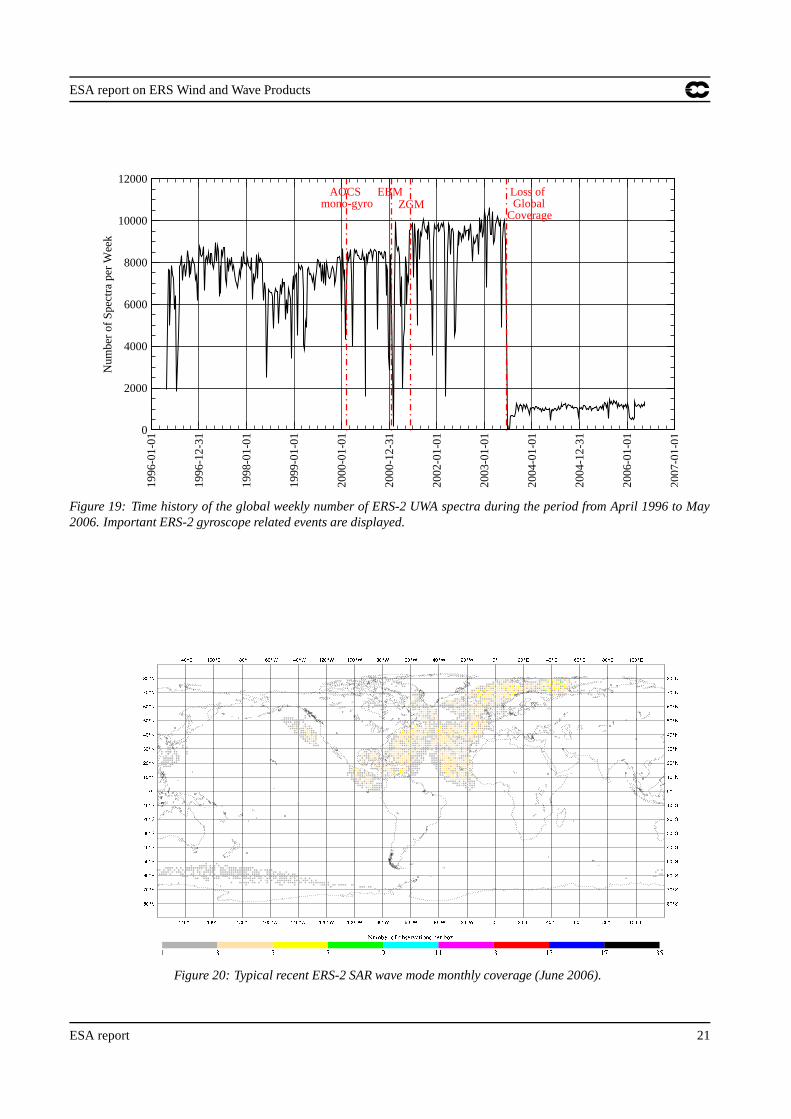
The loss of the global coverage due to the failure of the on-board low-bit rate tape recorders in June 2003reduced the number of observations received at ECMWF to about 13% of the full coverage data volume as canbe seen in Figure 19 which shows the global weekly number of SAR wave mode spectra processed at ECMWF.The current ERS-2 SAR coverage can be seen in Figure 20. As was done for the altimeter, the extra-tropicalNorthern Atlantic (north of latitude 20
�
N) is used for monitoring the FD SAR wave mode UWA product. Thisis very close to the bulk of the current coverage. The weekly number of SAR wave mode spectra in the NorthAtlantic since the beginning of the ERS-2 mission is shown in Figure 21. It is clear that the current coveragein the North Atlantic is slightly less than the nominal coverage. The difference is small and is due to the smallgap at the southern edge of the North Atlantic. The quality of the products in this area is investigated here.
4.2 ERS-2 SAR Wave Height in the North Atlantic
A long-term monitoring of the significant wave height computed from the inverted ERS-2 SAR spectra wasperformed. It is worthwhile mentioning that on 28 June 1998 the SAR inversion software was unable to properlyhandle the SAR data with the new calibration procedure introduced around that time. This was fixed with theimplementation of the ECWAM model change on 20 November 2000. Furthermore, SAR data have beenassimilated in the wave model since 13 January 2003. Further related events are mentioned in Section 4.4.
Figure 22 shows the time history of the daily bias of the significant wave height computed from the invertedSAR wave mode spectrum with respect to the model wave height in the North Atlantic since April 1996. Byignoring the period with the inversion bug (from 28 June 1998 to 20 November 2000) and the period with EBM(from 17 January 2001 to mid June 2001), it is possible to recognise a seasonal cyclic variation similar to thealtimeter SWH (i.e. with minima during the NH winter and maxima during the summer). It is clear that thebias behaviour since the loss of the global coverage is similar to that of 2-3 years before.
20 ESA report
ESA report on ERS Wind and Wave Products
1996
-01-
01
1996
-12-
31
1998
-01-
01
1999
-01-
01
2000
-01-
01
2000
-12-
31
2002
-01-
01
2003
-01-
01
2004
-01-
01
2004
-12-
31
2006
-01-
01
2007
-01-
01
0
2000
4000
6000
8000
10000
12000
Num
ber
of S
pect
ra p
er W
eek
AOCSmono-gyro
EBMZGM
Loss of GlobalCoverage
Figure 19: Time history of the global weekly number of ERS-2 UWA spectra during the period from April 1996 to May2006. Important ERS-2 gyroscope related events are displayed.
Figure 20: Typical recent ERS-2 SAR wave mode monthly coverage (June 2006).
ESA report 21

ESA report on ERS Wind and Wave Products
01-0
1-19
96
31-1
2-19
96
01-0
1-19
98
01-0
1-19
99
01-0
1-20
00
31-1
2-20
00
01-0
1-20
02
01-0
1-20
03
01-0
1-20
04
31-1
2-20
04
01-0
1-20
06
01-0
1-20
07
0
200
400
600
800
1000
1200
1400
1600
Num
ber
of
SA
R O
bser
vatio
ns p
er W
eek
Figure 21: Time history of the 7-day running average of daily number of SAR wave mode spectra in the North Atlanticsince 1 January 1996. Date of loss of global coverage is represented by a red thick vertical line.
01-0
1-19
96
31-1
2-19
96
01-0
1-19
98
01-0
1-19
99
01-0
1-20
00
31-1
2-20
00
01-0
1-20
02
01-0
1-20
03
01-0
1-20
04
31-1
2-20
04
01-0
1-20
06
01-0
1-20
07
-0.2
-0.1
0.0
0.1
0.2
ER
S-2
SA
R S
WH
Bia
s =
ER
S -
WA
M
(m
)
Figure 22: Time history of the 7-day running average of daily bias of SAR wave mode significant wave height with respectto wave model in the North Atlantic since 1 January 1996. Date of loss of global coverage is represented by a red thickvertical line.
22 ESA report

ESA report on ERS Wind and Wave Products
01-0
1-19
96
31-1
2-19
96
01-0
1-19
98
01-0
1-19
99
01-0
1-20
00
31-1
2-20
00
01-0
1-20
02
01-0
1-20
03
01-0
1-20
04
31-1
2-20
04
01-0
1-20
06
01-0
1-20
07
0.10
0.12
0.14
0.16
0.18
0.20
0.22
ER
S-2
SA
R S
WH
Sca
tter
Inde
x w
.r.t.
WA
M
Figure 23: Time history of the 7-day running average of daily scatter index of SAR wave mode significant wave heightwith respect to wave model in the North Atlantic since 1 January 1996. Date of loss of global coverage is represented bya red thick vertical line.
Figure 23 shows the time history of the daily scatter index of the SWH of the inverted SAR wave mode productwith respect to the operational wave model in the North Atlantic since April 1996. There tends to be a kindof seasonal cycle (in phase with the bias cycle) of variation in SI after the recovery from the EBM using theZGM. This seasonal cycle continued after the loss of the global coverage. Furthermore, the general trend of SIreduction continued over the period of limited coverage. Even the errors became smaller than ever; especiallyduring the winter. This may be a consequence of assimilating the SAR wave mode product in the ECMWFoperational wave model since 13 January 2003. A step change in SI can not be seen at that specific date.However, the SI peak values started to be the lowest during the NH summer of 2003.
4.3 Global ERS-1 SAR Significant Wave Height
Figure 24 shows the time history of the weekly number of ERS-1 FD SAR Wave Mode spectra (UWA) productsover the entire globe during the period from April 1993 to April 1996. There is no UWA data available atECMWF before April 1993. The number of observations increased slightly towards the end of 1993.
Figure 25 shows the time history of the weekly bias and scatter index of the SWH derived from the invertedERS-1 SAR spectra with respect to the operational ECMWF wave model during the period from April 1993to April 1996. The bias started at a level of about 27 cm before it increased linearly to about 44 cm duringJuly 1993. The reason of this change could not be correlated with any model or SAR related changes. Anotherlinear increase occurred during Phase D (the Second Ice Phase). The bias then fluctuated around 50 cm. Thebeginning of Phase G (the Second Multi-Disciplinary Phase) witnessed another bias increase to the level of 60cm. It is clear that almost all phase changes were associated with a local bias change (drop).
ESA report 23

ESA report on ERS Wind and Wave Products
1992
-12-
31
1994
-01-
01
1995
-01-
01
1996
-01-
01
1996
-12-
31
0
2000
4000
6000
8000
10000
12000
Num
ber
of
spe
ctra
per
wee
k
Phase C Phase D
Phase E Phase F Phase G
Figure 24: Time history of the 5-week running average of weekly number of ERS-1 UWA spectra during the period fromApril 1993 to April 1996. Various ERS-1 phases are displayed.
On the other hand, the SI values were small (about 21%) at the beginning. Gradual, but small, increase of SIcan be noticed. A significant SI jump happened at the beginning of Phase G together with the last bias jumpmentioned above. The SI exceeded 32% during the period from May to September 1995.
It should be noted that one can not rule out the impact of possible undocumented model changes on the observedchanges in Figure 25.
4.4 Global ERS-2 SAR Significant Wave Height
The time history of the weekly number of global ERS-2 SAR Wave Mode spectra products during the periodfrom April 1996 to May 2006 is shown in Figure 19. It should be noted that the LBR data coverage of ERS-2 was significantly reduced after the failure of the on-board tape recorders on 21 June 2003. Therefore, asdescribed earlier, any comparison after that date does not represent the global situation.
Figure 26 shows the time history of the global weekly bias and scatter index of the SWH computed from ERS-2 SAR wave mode spectra with respect to the operational ECMWF wave model during the period from April1996 to May 2006. It is worthwhile reminding that on 28 June 1998 a change in the SAR calibration procedureadversely impacted the SAR inversion process. This was fixed on 20 November 2000. The impact of this bugcan be clearly seen in Figure 26. Unfortunately, less than two months after the recovery from this bug, thespacecraft lost its gyroscopes on 17 January 2001 and was piloted, as a result, in the EBM. This resulted ina degraded UWA product during the period of EBM as can be clearly seen in Figure 26. The introduction ofthe ZGM later that year (June 2003), restored the UWA quality. The loss of the global coverage in June 2003limited the data to be mainly in the Northern Hemisphere. This fact is reflected into a strong seasonal bias cycleand a mild SI cycle both in phase. Another point to note is the gradual reduction of the SI by time.
24 ESA report

ESA report on ERS Wind and Wave Products
1992
-12-
31
1994
-01-
01
1995
-01-
01
1996
-01-
01
1996
-12-
31
0.00
0.20
0.40
0.60
0.80
SI
or
B
ias
(m
)
BiasSI
Phase C Phase D
Phase E Phase F Phase G
Figure 25: Time history of the 5-week running average of weekly global bias and scatter index of ERS-1 SAR significantwave height with respect to the operational ECMWF wave model during the period from April 1993 to April 1996. VariousERS-1 phases are displayed.
1996
-01-
01
1996
-12-
31
1998
-01-
01
1999
-01-
01
2000
-01-
01
2000
-12-
31
2002
-01-
01
2003
-01-
01
2004
-01-
01
2004
-12-
31
2006
-01-
01
2007
-01-
01
-0.20
-0.10
0.00
0.10
0.20
0.30
Bia
s (
m)
or
SI
SIBias
AOCSmono-gyro
EBM
ZGM
Inve
rsio
n B
ug R
emov
ed
SAR
Inv
ersi
on B
ug
Loss of GlobalCoverage
Figure 26: Time history of the 5-week running average of weekly global bias and scatter index of ERS-2 SAR signifi-cant wave height with respect to the operational ECMWF wave model during the period from April 1996 to May 2006.Important ERS-2 gyroscope related events and relevant model changes are displayed.
ESA report 25

ESA report on ERS Wind and Wave Products
J1991
A J O J1992
A J O J1993
A J O J1994
A J O J1995
A J O J1996
A J O J1997
A J O J1998
A J O J1999
A J O J2000
A J O J2001
A J O J2002
A J O J2003
A J O J2004
A J O J2005
A J O J2006
A0
2
4
6
8
10
Vo
lum
e (M
Byt
e)
for NRT ERS1 (RED) and ERS2 (BLUE) and off-line ERS2 (BLACK) data Daily data volume (light colours) and one-month moving average (dark colours)
MAGICS 6.10 noatun - dal Wed Jul 12 16:27:31 2006
Figure 27: Volume of received ERS-1 and ERS-2 UWI data at ECMWF subject to the data cut-off time in Mbyte per day.
5 The Scatterometer UWI product
5.1 Overview
The AMI instrument on board ERS-2, and previously ERS-1, obtains backscatter measurements from threeantennas, illuminating a swath of 500 km, in which 19 nodes define a 25 km product (for details on configurationand geometry see Attema, 1986). From these backscatter triplets, two wind solutions are retrieved one ofwhich is reported in a by ESA disseminated near-real time product, called UWI. For this the geophysical modelfunction CMOD4 (Stoffelen and Anderson, 1997) is used.
ERS-1 was launched on 17 July 1991 and has provided scatterometer data from September 1991 until December1999. At ECMWF, ERS-1 UWI data was received from 9 May 1991 to 3 June 1996 (red curve in Figure 27),i.e., including some pre-launch test data from 9 May to 4 July 1991. In April 1995 ERS-2 was launchedand is still operational. At ECMWF some preliminary data was received on 24 April 1995, while operationaldata flow started on 22 November 1995 (left-hand blue curve in Figure 27). Due to an on-board anomaly inJanuary 2001, ESA was forced to suspend data dissemination between 18 February 2001 and 21 August 2003.However, off-line data was obtained from ESRIN between 12 December 2001 and 7 November 2003 (blackcurve in Figure 27). Two months before public re-dissemination, ERS-2 had lost its storage capacity of LBRdata, including scatterometer data. After this event, data only remained available when in contact with a groundstation. As a consequence, global coverage was lost for the newly disseminated stream, resulting in much lowerdata volumes (right-hand blue curve in Figure 27).
Within the framework of various contracts with ESA and ESRIN, ECMWF has been monitoring UWI data fora number of years. By passing derived scatterometer winds to the ECMWF operational assimilation system(initially passively, since January 1996 actively), an accurate comparison with model winds can be obtained.Findings of such comparison are, amongst other quality checks, recorded in cyclic reports on 5-weekly inter-vals. Elements of these reports are described in Section 5.2.
A summary of the monitoring of the entire ERS-2 period will be presented in Section 5.3. It includes a com-parison with QuikSCAT data. Seasonal trends in wind speed bias will be discussed in Section 5.4.
26 ESA report

ESA report on ERS Wind and Wave Products
Besides being used in the operational data assimilation system, ERS-1 and ERS-2 data have been assimilatedin the ECMWF 40-year reanalysis (ERA-40, Uppala et al. , 2005). In Section 5.5 results of a triple collocationstudy of assimilated ERS-1 and ERS-2 winds (1 January 1993 to January 2001), ERA-40 first-guess modelwinds, and height-corrected buoy data will be presented.
At ECMWF and KNMI the improved geophysical model function CMOD5 had been developed some timeago (Hersbach 2003, Hersbach et al. 2004b). In Section 5.6 preliminary results on a refit of CMOD5 will bediscussed, that resolves residual biases relative to buoy wind data.
At ESRIN, the entire ERS-1 and ERS-2 record is currently being reprocessed, and for this a new processor(named ASPS20) has been developed (Crapolicchio et al. 2004). As a check, at ECMWF, some test data fromthis processor was compared with archived UWI data. Results are presented in Section 5.7.
5.2 5-weekly cyclic UWI ERS-2 monitoring reports
The routine monitoring of the ERS-2 UWI product at ECMWF is summarized in the form of 5-weekly cyclicreports. At http://earth.esa.int/pcs/ers/scatt/reports/ecmwf/, these reports are available from Cycle 41 (start date14 July 1998) up to, at the time of this writing, Cycle 116 (end date 26 June 2006).
Up to Cycle 60 (nominal period) the UWI product has been compared with ECMWF first-guess winds as avail-able within the assimilation system. These FGAT (first-guess at appropriate time) winds are well collocatedwith the scatterometer observation time and location. From Cycle 69 onwards, e.g., with the start of the re-ception of offline data from ESRIN, collocation was performed with archived first-guess wind fields instead(available at 3-hourly resolution; and will be called FG winds). Collocation errors are slightly larger, but on theother hand it enables the monitoring of data that does not pass pre-assimilation quality control.
From Cycle 69 onwards, the quality of winds inverted on the basis of CMOD5 are monitored as well. AtECMWF, such retrieved ERS-2 scatterometer winds have been assimilated from 9 March 2004 onwards.
The ECMWF scatterometer cyclic monitoring reports contain the following elements:
� An introduction, giving a general summary of the quality of the UWI data and trends w.r.t. previouscycles. Data coverage, and interruptions in data reception are listed. Also, since Cycle 69 (12 November2001) it is mentioned whether there was an enhancement of solar activity, and whether it could haveaffected the UWI wind product. Finally, it is informed whether the ECMWF assimilation system haschanged and whether this had an anticipated impact on the quality of the ECMWF surface winds.
� A section giving a detailed description of performance during the cycle. It includes the following plots.
� Evolution of 5-weekly averaged performance of the cone distance, bias and standard deviation of UWIand CMOD4 wind speed and direction compared to ECMWF FG winds starting from Cycle 69. The plotfor Cycle 116 is given in Figure 28.
� Data coverage and geographical averages of UWI wind speed, and relative bias and standard deviationcompared to ECMWF FG winds (Cycle 91 onwards; for Cycle 116, see Figure 29).
� Backscatter (σ0) bias for the three beams (fore, mid, aft) as function of across-node number (1 to 19) andstratified with respect to ascending and descending tracks:
dz ��� z � � � zCMOD � θ � FGAT ����
ESA report 27

ESA report on ERS Wind and Wave Products
Figure 28: Evolution of the performance of the ERS-2 scatterometer averaged over 5-weekly cycles from 12 December2001 (Cycle 69) to 26 June 2006 (end Cycle 116) for the UWI product (solid, star) and de-aliased winds based on CMOD4(dashed, diamond). Results are based on data that passed the UWI QC flags. For Cycle 85 two values are plotted; thefirst value for the global set, the second one for the regional set (see text for more details). Dotted lines represent valuesfor Cycle 59 (5 December 2000 to 17 January 2001), i.e. the last stable cycle of the nominal period. From top to bottompanel are shown the normalized distance to the cone (CMOD4 only) the standard deviation of the wind speed compared toFG winds, the corresponding bias (for UWI winds the extreme inter-node averages are shown as well), and the standarddeviation of wind direction compared to FG.
28 ESA report

ESA report on ERS Wind and Wave Products
where z � σ 0 � 6250 , and θ the node and beam-dependent incidence angle. This bias depends on the under-
lying model function. Results are produced on the basis of CMOD4. Trends in the inter-node and inter-beam relationship indicate changes in the antenna patterns, because trends in the normalizing ECMWFwinds would appear as integral shifts. Examples (Cycle 110 and 116) are given in Figure 30.
� Time series of the difference between the fore and aft incidence angle of node 10 (Cycle 81 onwards), andthe UWI kp-yaw quality flag (Cycle 88 onwards). Asymmetries indicate errors in yaw attitude control.
� Plots of time series of quantities averaged over 6-hourly data batches and stratified w.r.t. six classes ofnodes (1-2, 3-4, 5-7, 8-10, 11-14 and 15-19) of
– The normalized distance to the cone, the fraction of rejected data on the basis of CMOD4 inversion,ESA flags or ECMWF land and sea-ice mask, and the total number of received data over sea.
– Bias and standard deviation of UWI versus ECMWF first-guess winds for wind speed and direction.
– The same for CMOD4 winds as inverted at ECMWF from level 1b.
� Global plots of locations where UWI winds were more than 8 ms� 1 weaker or stronger than ECMWF
FG winds (included from Cycle 79). Usually two specific cases are highlighted in a separate plot.
� Accumulated histograms (scatter plots) between UWI and ECMWF first-guess wind speed and direction.Scatter plots for FG winds versus de-aliased CMOD4 winds and CMOD5-based winds have been pro-duced from Cycle 74 onwards. Examples for a one-year accumulation period (1 July 2005 to 30 June2006) are presented in Figure 31.
� Time series for at ECMWF assimilated CMOD5 winds, and QuikSCAT winds relative to ECMWF FGATwinds for a region covering the North Atlantic and part of Europe (Cycle 94 onwards; for Cycle 116 seeFigure 33).
5.3 General Overview for ERS-2
22 November 1995 - 19 March 1996Pre calibration phase. Large but constant σ0 biases were encountered.
19 March 1996 - 6 August 1996End of commissioning phase. A thorough calibration has resulted in revised look-up tables. Scatterometer datafrom ERS-2 (bias-corrected CMOD4 winds) is included in the ECMWF assimilation system on 1 June 1996,replacing the assimilation from ERS-1 that had been used from 30 January 1996. Details may be found inIsaksen and Janssen (2004).
6 August 1996 - 18 June 1997Due to an erroneous switch to a redundant calibration subsystem σ0 values increase by 0.2 dB, leading to windbiases � 0 � 5ms
� 1 .
18 June 1997 - 17 January 2001 (Cycle 22 to Cycle 60)Nominal period. Backscatter values return to old, well-calibrated levels.
The performance of the UWI product is stable, although in the fall of 2000 there are some problems with thefunctioning of several of the six gyroscopes on-board the spacecraft. On average, backscatter levels are around0.5 dB too low, leading to winds that are on average 0.7-0.8 ms
� 1 slower than FGAT winds. Although the inter-node and inter-beam sigma biases are small, the UWI wind-speed bias does depend on node number (from
ESA report 29

ESA report on ERS Wind and Wave Products
80°S80°S
70°S 70°S
60°S60°S
50°S 50°S
40°S40°S
30°S 30°S
20°S20°S
10°S 10°S
0°0°
10°N 10°N
20°N20°N
30°N 30°N
40°N40°N
50°N 50°N
60°N60°N
70°N 70°N
80°N80°N
160°W
160°W 140°W
140°W 120°W
120°W 100°W
100°W 80°W
80°W 60°W
60°W 40°W
40°W 20°W
20°W 0°
0° 20°E
20°E 40°E
40°E 60°E
60°E 80°E
80°E 100°E
100°E 120°E
120°E 140°E
140°E 160°E
160°E
average from 2006052300 to 2006062618 GLOB:3.15NOBS ( ERS-2 CMOD5 ), per 12H, per 125km box
0.1
1
2
4
8
16
32
80°S80°S
70°S 70°S
60°S60°S
50°S 50°S
40°S40°S
30°S 30°S
20°S20°S
10°S 10°S
0°0°
10°N 10°N
20°N20°N
30°N 30°N
40°N40°N
50°N 50°N
60°N60°N
70°N 70°N
80°N80°N
160°W
160°W 140°W
140°W 120°W
120°W 100°W
100°W 80°W
80°W 60°W
60°W 40°W
40°W 20°W
20°W 0°
0° 20°E
20°E 40°E
40°E 60°E
60°E 80°E
80°E 100°E
100°E 120°E
120°E 140°E
140°E 160°E
160°E
average from 2006052300 to 2006062618 GLOB:-0.43BIAS ( ERS-2 CMOD5 vs FIRST-GUESS ), in m/s.
-5
-2.5
-1
-0.5
0
0.5
1
2.5
5
80°S80°S
70°S 70°S
60°S60°S
50°S 50°S
40°S40°S
30°S 30°S
20°S20°S
10°S 10°S
0°0°
10°N 10°N
20°N20°N
30°N 30°N
40°N40°N
50°N 50°N
60°N60°N
70°N 70°N
80°N80°N
160°W
160°W 140°W
140°W 120°W
120°W 100°W
100°W 80°W
80°W 60°W
60°W 40°W
40°W 20°W
20°W 0°
0° 20°E
20°E 40°E
40°E 60°E
60°E 80°E
80°E 100°E
100°E 120°E
120°E 140°E
140°E 160°E
160°E
average from 2006052300 to 2006062618 GLOB:1.22STDV ( ERS-2 CMOD5 vs FIRST-GUESS ), in m/s.
0
0.5
0.75
1
1.5
2.5
5
Figure 29: Average number (top) of observations per 12H and per N80 reduced Gaussian grid box ( � 125 km), relativebias (middle) respectively standard deviation (lower panel) compared to ECMWF FG 10-meter winds, ( � 125 km) ofUWI winds that passed quality control at ECMWF for data in Cycle 116 (23 May - 26 June 2006). Only data are plottedfor grid cells that contained at least 5 observations.
30 ESA report

ESA report on ERS Wind and Wave Products
-1.1 ms� 1 for low to -0.6 ms
� 1 for high incidence angle). It is induced by imperfections in the CMOD4 modelfunction (and do not appear for CMOD5). Standard deviation between UWI and FGAT winds are around 1.6ms
� 1 . For Cycle 59, values of the average cone distance, (UWI - FGAT) and (CMOD4 - FGAT) statistics aredisplayed by the horizontal dotted lines in Figure 28.
17 January 2001 - July 2001 (Cycle 60 to 65)As a result of the on-board failure there are no gyroscopes left for the platform’s attitude control. The controlsystem is switched to Extra Back-up Mode. The dissemination of scatterometer data is suspended after 2February 2001; empty cyclic reports are made for Cycles 62 to 68.
July 2001 - 12 December 2001 (Cycle 65 to 69)Introduction of the Zero-Gyro Mode (ZGM). Satellite pointing is achieved through payload data and the digitalearth sensor. Although pitch and roll can be controlled accurately, large errors in the yaw attitude (severaldegrees) still occur. Such errors especially affect the quality of the scatterometer measurements. Disseminationof scatterometer data remains suspended.
12 December 2001 - 4 February 2003 (Cycle 69 to 81).Restart of dissemination of UWI data, however, to a restricted group of users only. At ECMWF, the monitoringis resumed. Existing tools are updated where necessary.
Large errors in yaw, which especially seem to occur around periods of enhanced solar activity, have a largenegative impact on the data quality. During these events, part of the backscatter signal is destroyed, which,after inversion, results in far too low winds. Peaks of more than -3 ms
� 1 frequently occur, especially in January2002 (Cycle 70), which marks a period of considerable solar activity. These incorrect data are also visible in thescatter diagrams of UWI versus FG wind speed as anomalously large numbers of collocations between strongECMWF winds and weak UWI winds. For later cycles the situation improves.
Initially, also extremely large negative biases are observed in the backscatter levels, including data that wasless affected by yaw errors. Large inter-node and inter-beam differences induce large cone distances. Thesituation is worst for Cycle 70 but later slowly improves. However, the increasing negative bias towards highernodes remains. In line with the average reduction in σ0 bias, the cone distance and wind-speed biases graduallyimprove (see Figure 28).
For the random error of the UWI and CMOD4 wind speeds a similar trend is observed: worst for Cycle 70(almost 2 ms
� 1 ) and then first improving rapidly and later stabilizing. From Cycle 75 onwards its level isaround the value obtained for the nominal period (see Figure 28). In general best results are obtained for windsinverted on the basis of CMOD5. Both the negative bias level and standard deviation are smaller for suchderived winds.
The performance in wind direction is found to be much less affected. Although initially wind direction performssomewhat worse, at Cycle 72 it is on the level of the nominal period, and after Cycle 75 it has even becomebetter (see lower panel of Figure 28).
4 February 2003 - 22 June 2003 (Cycle 81 to 85)Start of the validation phase of ESACA, the new processor. Aim of this complete revision of the originalLRDPF, was to bring the quality of the UWI product back to its nominal level. It is capable of the interpretationof on-board filter characteristics appropriately according to an estimation of the yaw attitude error. Duringthe test phase, ESACA data is distributed for Kiruna station only, which leads to daily data gaps betweenapproximately 21 UTC and 06 UTC.
The new de-aliasing algorithm, being part of ESACA, (and developed at DNMI) appears to perform well.The UWI winds agree considerably more often to the wind solution that is closest to the ECMWF FG wind
ESA report 31

ESA report on ERS Wind and Wave Products
direction. Values of standard deviations drop from 50 to less than 30 degrees (see Figure 28).
The UWI winds do not coincide anymore with one of the two solutions from the CMOD4 inversion at ECMWF.At ECMWF inverted CMOD4 winds appear to be of much higher quality than the by ESRIN disseminatedUWI winds (see Figure 28). At ESRIN, the cause for this non-ideal situation is tracked down quickly. At thebeginning of April 2003 appropriate corrections to ESACA are implemented and since then UWI winds arein line with CMOD4 again (though not yet for Kiruna station; i.e., the discrepancy in winds remains for thedata as received at ECMWF). The standard deviation w.r.t. FGAT winds are below 1.50 ms
� 1 , i.e., about 0.1ms
� 1 better than it used to be during the nominal period.
Large fractions of high kp values are found, especially for nodes at high incidence angles (more than 50%).Consideration between the (UK) MetOffice and ESRIN reveals that there is a problem with the BUFR encodingalgorithm. A solution is formulated and implemented (again, not yet at Kiruna).
In the near range the fore and aft beam show large negative biases in the average backscatter levels. As a result,very large negative wind-speed biases are found for low nodes (-1.6 ms
� 1 ). At ESRIN its cause is identifiedand resolved (though, not visible at Kiruna). Apart from the initially large near-range biases, the inter-nodeand inter-beam differences in backscatter levels are small. Their level is comparable to that during the nominalperiod.
The incidence angles between the fore and aft beam are not equal anymore. They now show a rapid vari-ation in time and peaks up to 7 degrees are observed. This asymmetry is a direct result of errors in yawattitude. A large anomaly on April 1 2003 (while the Earth was inside a gusty solar wind stream, source:www.spaceweather.com) results in low-quality winds. This event illustrates the potential usefulness of a yawflag in the UWI product.
Along with improved quality of the CMOD4 winds, the normalized distance to the cone is now below the levelof the nominal period.
22 June 2003 - 21 August 2003 (Cycle 85 to 87)On 22 June 2003 the second Low Bit-Rate recorder on-board ERS-2 fails, and is found to be beyond repair.As the first recorder had become unusable in December 2002, this means that now there is no facility left tostore LBR data, including scatterometer data. After a data-void period of three weeks, data flow is resumed on16 July 2003, however, only for observations for which there is a direct contact with a ground station. For theKiruna test data received at ECMWF, this means that coverage is limited to the Atlantic north of 40
�
N, makingstatistics very sparse.
21 August 2003 - 26 June 2006 (Cycle 88 to 116)On 21 August 2003, the public dissemination of UWI data is restarted. This fortunate event makes an end to therestricted distribution. From this date onwards data is received in the original manner (via the UK Met-Office),and is stored in the usual ECMWF analysis-input archives (the restricted data had been archived at a lessaccessible location). The original monitoring in the assimilation system (e.g., comparison with FGAT winds)is restored. However, cyclic reports are still based on the off-line monitoring (FG winds), since it includes datathat is rejected in an early stage of the assimilation system. Besides Kiruna station, data is now also receivedfrom Maspalomas, Gatineau and Prince Albert, which, bearing in mind the loss of the LBR recorders, resultsin a coverage over the North Atlantic, part of the Mediterranean, the Gulf of Mexico, and a small part of thePacific north-west from the US and Canada. An initial gap in the North Atlantic is resolved on 15 January2004, when a station at West Freugh (Scotland) is included. Coverage in the Caribbean is obtained by a stationat Miami (February 2005), in the Chinese Sea by a station at Beijing (July 2005), and partial coverage over theSouthern Hemisphere by the inclusion of McMurdo (Antarctica, June 2005) and Hobart (Tasmania, February2006) stations. All joined together lead to a (for Cycle 116) coverage as indicated in Figure 29. The areas
32 ESA report

ESA report on ERS Wind and Wave Products
15 20 25 30 35 40 45 50 55 60
Incidence Angle (degree)
-2
-1
0
1
B
ias
(dB
)
___ Fore _ _Mid ...Aft thin: Error Bar 567479 Entries, 55.9 % used (flat wind dir. dist.)
ASCENDING TRACKSERS-2 obs. from 28/11/2005 21:04 UTC to 02/01/2006 20:58 UTC
BIAS: (s0obs**0.625)/(s0fg3h**0.625)
15 20 25 30 35 40 45 50 55 60
Incidence Angle (degree)-2
-1
0
1
B
ias
(dB
)
___ Fore _ _Mid ...Aft thin: Error Bar 391786 Entries, 49.7 % used (flat wind dir. dist.)
DESCENDING TRACKSERS-2 obs. from 28/11/2005 21:04 UTC to 02/01/2006 20:58 UTC
BIAS: (s0obs**0.625)/(s0fg3h**0.625)
15 20 25 30 35 40 45 50 55 60
Incidence Angle (degree)
-2
-1
0
1
B
ias
(dB
)
___ Fore _ _Mid ...Aft thin: Error Bar 715312 Entries, 57.2 % used (flat wind dir. dist.)
ASCENDING TRACKSERS-2 obs. from 22/05/2006 21:01 UTC to 26/06/2006 20:56 UTC
BIAS: (s0obs**0.625)/(s0fg3h**0.625)
15 20 25 30 35 40 45 50 55 60
Incidence Angle (degree)-2
-1
0
1
B
ias
(dB
)
___ Fore _ _Mid ...Aft thin: Error Bar 617722 Entries, 61.6 % used (flat wind dir. dist.)
DESCENDING TRACKSERS-2 obs. from 22/05/2006 21:01 UTC to 26/06/2006 20:56 UTC
BIAS: (s0obs**0.625)/(s0fg3h**0.625)
Figure 30: Ratio of� σ 0 � 625
0����� CMOD4 � FGAT � 0 � 625 � converted in dB for the fore beam (solid line), mid beam
(dashed line) and aft beam (dotted line), as a function of incidence angle for and ascending tracks of data within Cycles111 (left panel) and 116 (right panel). The thin lines indicate the error bars on the estimated mean.
covered by Miami and Beijing station allow for the accurate observation of a number of tropical cyclones.
The recording by separate ground stations means that in certain areas observations are reported more thanonce. For each ground station gridding into 25-km cells and de-aliasing is performed separately. It is foundthat overlapping cells may be dislocated (by 12.5 km), and that regularly not the same wind solution is selectedfor all ground stations.
The operational ESACA processor has resolved all non-optimal features that had been detected during thevalidation period. Data quality is found to be high, although the cone distance has increased and is now 10%higher than for nominal data (see top panel of Figure 28). Assimilation experiments with winds inverted on thebasis of CMOD5, show a small positive impact in global forecast skill (Hersbach et al. 2004a). It leads to there-introduction of ERS-2 scatterometer data in the ECMWF assimilation system on 8 March 2004.
An original flag for high kp values is now also set for yaw attitude errors exceeding 2 degrees. It appears towork well and a close correlation with the asymmetry in incidence angle is observed.
Since the loss of global coverage, a seasonal trend has been introduced in the now regional data set, makingobjective monitoring more difficult. A clear example of such a trend is observed for the relative standarddeviation of the UWI wind speed compared to FG winds (see second panel of Figure 28); a more intense andvolatile wind climate in winter time will naturally lead to an increased RMSE.
A seasonal trend also appears for bias levels of both wind speed and backscatter. For backscatter, bias patternsare found to be flat in winter time (at levels that are less negative than for nominal data), but large asymme-tries emerge during summer. Typical examples for this consistent yearly trend are given in Figure 30. Forwind speed, bias relative to ECMWF FG winds, are found to be (like backscatter) most negative around July( � 1 � 1ms
� 1 ) and least negative around January ( � 0 � 7ms� 1 ). In the next Section, this issue will be studied
in some detail.
Yearly averaged (over all 19 nodes) UWI winds are about 0 � 8 � 0 � 9m s� 1 biased low compared to ECMWF
FG winds (see e.g., top left-hand panel of Figure 31 for the period July 2005 - June 2006). This is slightlymore negative than for nominal data (before January 2001), and is probably due to a gradual slight increasein average wind speed of the ECMWF first-guess winds. This trend emerges, e.g., from longterm monitoringof QuikSCAT winds and of buoy winds (not shown). For CMOD5, average wind bias is around � 0 � 35ms
� 1 .
ESA report 33

ESA report on ERS Wind and Wave Products
0 5 10 15 20 25 30 35
Wind Speed (m/s) 3-hourly First-Guess�0
5
10
15
20
25
30
35
Win
d S
peed
(m
/s)
U
WI
W
ind
m(y-x)= -0.86 sd(y-x)= 1.51 sdx= 3.76 sdy= 3.55 pcxy= 0.957 = 11286658, db contour levels, 5 db step, 1st level at 15.5 db
from 2005070100 to 2006063018ECMWF 3-hourly First-Guess winds versus UWI winds
0 5 10 15 20 25 30 35
Wind Speed (m/s) 3-hourly First-Guess�0
5
10
15
20
25
30
35
Win
d S
peed
(m
/s)
C
MO
D5
Win
d
m(y-x)= -0.36 sd(y-x)= 1.47 sdx= 3.69 sdy= 3.63 pcxy= 0.959 = 10955520, db contour levels, 5 db step, 1st level at 15.4 db
from 2005070100 to 2006063018ECMWF 3-hourly First-Guess winds versus CMOD5 winds
0 45 90 135 180 225 270 315 360
Wind Direction (deg) 3-hourly First-Guess�0
45
90
135
180
225
270
315
360
Win
d D
irect
ion
(deg
) U
WI
W
ind
m(y-x)= -2.67 sd(y-x)= 32.78 sdx=106.26 sdy=106.80 pcxy= 0.976 = 9045094 ( |f| gt 4.00 m/s ), db contour levels, 5 db step, 1st level at 14.6 db
from 2005070100 to 2006063018ECMWF 3-hourly First-Guess winds versus UWI winds
0 45 90 135 180 225 270 315 360
Wind Direction (deg) 3-hourly First-Guess�0
45
90
135
180
225
270
315
360
Win
d D
irect
ion
(deg
) C
MO
D5
Win
d
m(y-x)= -2.27 sd(y-x)= 20.07 sdx=105.35 sdy=104.59 pcxy= 0.991 = 9517396 ( |f| gt 4.00 m/s ), db contour levels, 5 db step, 1st level at 14.8 db
from 2005070100 to 2006063018ECMWF 3-hourly First-Guess winds versus CMOD5 winds
Figure 31: Two-dimensional histogram of UWI (left hand panels) or de-aliased CMOD5 (right hand panels) relative toECMWF FG for wind speed (top panels) and wind direction (lower panels) over the one-year period from 1 July 2005 to30 June 2006. Blue circles denote averages for bins in the x-direction, and red squares averages for bins in the y-direction.
34 ESA report

ESA report on ERS Wind and Wave Products
30°
N 30°N
32°N
32°
N
136°E 138°E 140°E
SAOLA 20050924 13:15 UTCCMOD5 winds (red) versus FGAT winds (blue)
28°N
28°
N30
°N 30°N
32°N
32°
N
72°W 70°W 68°W
20050409 15:10 UTCCMOD4 winds (red) versus FGAT winds (blue)
Figure 32: Two examples for situations where scatterometer and ECMWF winds differ significantly.
This relative bias seems fairly independent on wind speed, as e.g. can be seen from the histogram displayedin the top right-hand panel of Figure 31. The one-year accumulated relative standard deviation of UWI windsis about 0.1 ms �
1 lower than for nominal data (1.5 ms �1 versus 1.6 ms �
1 ), but this can be the result of theomission of the strong winds in the Southern Hemispheric storm tracks, combined with the gradually improvedquality of ECMWF winds.
As observed during the ESACA test phase, the quality of UWI wind direction is (as a result of the improvedde-aliasing algorithm) superior to that of nominal data (see lower panel of Figure 28). Nevertheless, incorrectwind solutions are still frequently reported as can be seen from the lower panels of Figure 31. Occasionally,peaks of degraded performance occur, which usually can be traced back to temporarily missing input (modelwinds) in the ESACA de-aliasing software. Such peaks are not observed for at ECMWF de-aliased CMOD5winds.
A previously non-existing bias is observed for wind direction. On average, (de-aliased) ERS-2 winds arefound to be rotated by 3 degrees counter-clockwise compared to ECMWF first-guess fields. One reason forthis consistent bias appears the lack of cross-isobar flow (Hollingsworth 1994) at warm advection of ECMWFsurface winds. A similar, opposite, effect is found on the Southern Hemisphere, and, therefore, this bias isaveraged out in a global verification. A study for QuikSCAT data versus model winds may be found in Brownet al. 2005.
Locations for large differences between UWI (or CMOD5) winds are usually isolated. They often indicate me-teorologically active regions, for which UWI data and ECMWF model field show reasonably small differencesin phase and/or intensity. Tropical cyclones and frontal systems are typical candidates. One example is theobservation of typhoon Saola from Beijing ground station on 24 September 2005, which is displayed in theleft panel of Figure 32. Hardly affected by rain, the ERS-2 scatterometer winds are able to provide a detailedpicture. It shows that ECMWF first-winds are, besides suffering from a lack of cross-isobar flow, too weak nearthe cyclone centre.
Besides large differences that pin point errors in the ECMWF first-guess field, occasionally cases are observedin which UWI winds seem clearly incorrect. This is often manifested as odd patches within a surrounding wind
ESA report 35

ESA report on ERS Wind and Wave Products
J2004
F M A M J J A S O N D J2005
F M A M J J A S O N D J2006
F M A M J-1
-0.8
-0.6
-0.4
-0.2
0
0.2
0.4
0.6
BIA
S (
m/s
)
WIND SPEED, nodes 1-19, 15-day moving average, AREA= NATLERS2 scatterometer versus ECMWF FGAT (BLUE) and Analysis (RED)
J2004
F M A M J J A S O N D J2005
F M A M J J A S O N D J2006
F M A M J-1
-0.8
-0.6
-0.4
-0.2
0
0.2
0.4
0.6
BIA
S (
m/s
)
WIND SPEED, nodes 5-34, 15-day moving average, AREA= NATLQuikSCAT (50km) versus ECMWF FGAT (BLUE) and Analysis (RED)
MAGICS 6.10 noatun - dal Tue Aug 1 15:11:06 2006
Figure 33: Wind-speed bias relative to FG winds for actively assimilated ERS-2 winds (based on CMOD5) for nodes1-19 (top panel) respectively 50-km QuikSCAT (based on the QSCAT-1 model function and reduced by 4%) for nodes5-34 (lower panel), averaged over the area (20N-90N, 80W-20E), and displayed for the period 01 January 2004 - 26 June2006. Fat curves represent centred 15-day running means, thin curves values for 6-hourly periods. Vertical dashed bluelines mark ECMWF model changes.
field that looks sensible. An example is shown in the right-hand panel of Figure 32. Problems are found mostlikely to occur at light wind conditions relatively close to land, and at lower incidence angles in general.
5.4 Seasonal fluctuations in wind speed bias
The evolution in wind bias of the regional data set can also be well-observed from the monitoring of the windproduct as used in the ECMWF assimilation system. Figure 33 presents a time series for ERS-2 (based onCMOD5), and QuikSCAT data (50-km product based on QSCAT-1 model function, minus 4% bias correction)restricted to an area that is well-covered by ERS-2. It shows that a similar (though somewhat weaker) trendfor the regional ERS-2 data is also found for QuikSCAT data. This indicates that the variations have probablya geophysical nature, and therefore do not indicate changes in the ERS-2 antenna pattern. Several reasons forthe yearly trend can be suggested. One obvious contribution is the fact that a scatterometer measures wind viathe surface stress. Direct transformation from surface stress to 10-metre wind (called equivalent neutral winds)does not take local stability effects into account. Typically, in unstable conditions, equivalent neutral windsare about 0.2 ms
� 1 stronger, and vice versa for stable conditions. Since (ECMWF) model 10-metre winds do
36 ESA report
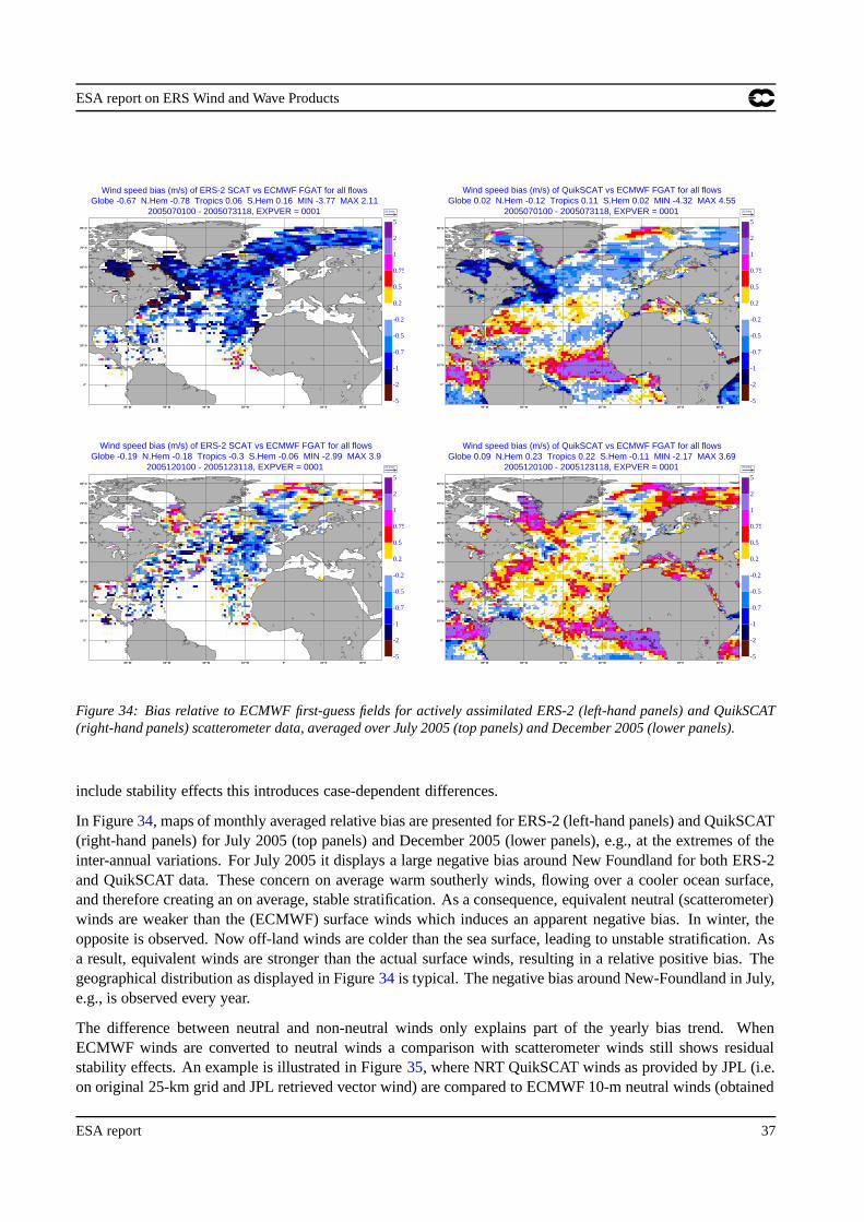
ESA report on ERS Wind and Wave Products
25.0m/s
0°0°
10°N 10°N
20°N20°N
30°N 30°N
40°N40°N
50°N 50°N
60°N60°N
70°N 70°N
80°N80°N
80°W
80°W 60°W
60°W 40°W
40°W 20°W
20°W 0°
0° 20°E
20°E 40°E
40°E
2005070100 - 2005073118, EXPVER = 0001 Globe 0.02 N.Hem -0.12 Tropics 0.11 S.Hem 0.02 MIN -4.32 MAX 4.55
Wind speed bias (m/s) of QuikSCAT vs ECMWF FGAT for all flows
-5
-2
-1
-0.75
-0.5
-0.2
0.2
0.5
0.75
1
2
5
25.0m/s
0°0°
10°N 10°N
20°N20°N
30°N 30°N
40°N40°N
50°N 50°N
60°N60°N
70°N 70°N
80°N80°N
80°W
80°W 60°W
60°W 40°W
40°W 20°W
20°W 0°
0° 20°E
20°E 40°E
40°E
2005120100 - 2005123118, EXPVER = 0001 Globe 0.09 N.Hem 0.23 Tropics 0.22 S.Hem -0.11 MIN -2.17 MAX 3.69
Wind speed bias (m/s) of QuikSCAT vs ECMWF FGAT for all flows
-5
-2
-1
-0.75
-0.5
-0.2
0.2
0.5
0.75
1
2
5
25.0m/s
0°0°
10°N 10°N
20°N20°N
30°N 30°N
40°N40°N
50°N 50°N
60°N60°N
70°N 70°N
80°N80°N
80°W
80°W 60°W
60°W 40°W
40°W 20°W
20°W 0°
0° 20°E
20°E 40°E
40°E
2005070100 - 2005073118, EXPVER = 0001 Globe -0.67 N.Hem -0.78 Tropics 0.06 S.Hem 0.16 MIN -3.77 MAX 2.11
Wind speed bias (m/s) of ERS-2 SCAT vs ECMWF FGAT for all flows
-5
-2
-1
-0.75
-0.5
-0.2
0.2
0.5
0.75
1
2
5
25.0m/s
0°0°
10°N 10°N
20°N20°N
30°N 30°N
40°N40°N
50°N 50°N
60°N60°N
70°N 70°N
80°N80°N
80°W
80°W 60°W
60°W 40°W
40°W 20°W
20°W 0°
0° 20°E
20°E 40°E
40°E
2005120100 - 2005123118, EXPVER = 0001 Globe -0.19 N.Hem -0.18 Tropics -0.3 S.Hem -0.06 MIN -2.99 MAX 3.9
Wind speed bias (m/s) of ERS-2 SCAT vs ECMWF FGAT for all flows
-5
-2
-1
-0.75
-0.5
-0.2
0.2
0.5
0.75
1
2
5
Figure 34: Bias relative to ECMWF first-guess fields for actively assimilated ERS-2 (left-hand panels) and QuikSCAT(right-hand panels) scatterometer data, averaged over July 2005 (top panels) and December 2005 (lower panels).
include stability effects this introduces case-dependent differences.
In Figure 34, maps of monthly averaged relative bias are presented for ERS-2 (left-hand panels) and QuikSCAT(right-hand panels) for July 2005 (top panels) and December 2005 (lower panels), e.g., at the extremes of theinter-annual variations. For July 2005 it displays a large negative bias around New Foundland for both ERS-2and QuikSCAT data. These concern on average warm southerly winds, flowing over a cooler ocean surface,and therefore creating an on average, stable stratification. As a consequence, equivalent neutral (scatterometer)winds are weaker than the (ECMWF) surface winds which induces an apparent negative bias. In winter, theopposite is observed. Now off-land winds are colder than the sea surface, leading to unstable stratification. Asa result, equivalent winds are stronger than the actual surface winds, resulting in a relative positive bias. Thegeographical distribution as displayed in Figure 34 is typical. The negative bias around New-Foundland in July,e.g., is observed every year.
The difference between neutral and non-neutral winds only explains part of the yearly bias trend. WhenECMWF winds are converted to neutral winds a comparison with scatterometer winds still shows residualstability effects. An example is illustrated in Figure 35, where NRT QuikSCAT winds as provided by JPL (i.e.on original 25-km grid and JPL retrieved vector wind) are compared to ECMWF 10-m neutral winds (obtained
ESA report 37

ESA report on ERS Wind and Wave Products
0 5 10 15 20 25 30 35
Wind Speed (m/s) ECMWF neutral FG0
5
10
15
20
25
30
35
Win
d S
peed
(m
/s)
JP
L Q
uikS
CA
T
m(y-x)= 0.67 sd(y-x)= 1.99 sdx= 3.79 sdy= 4.16 pcxy= 0.938ncol = 11958259, 5 db contour steps, 1st level at 15.8 db
AREA=NHEM From 2000120100 to 2001022818ECMWF neutral FG winds versus JPL QuikSCAT winds
0 5 10 15 20 25 30 35
Wind Speed (m/s) ECMWF neutral FG0
5
10
15
20
25
30
35
Win
d S
peed
(m
/s)
JP
L Q
uikS
CA
T
m(y-x)= 0.12 sd(y-x)= 2.25 sdx= 3.92 sdy= 3.96 pcxy= 0.915ncol = 1613253, 5 db contour steps, 1st level at 7.1 db
AREA=NHEM From 2000120100 to 2001022818ECMWF neutral FG winds versus JPL QuikSCAT winds
Figure 35: Scatter plot of NRT NESDIS QuikSCAT product versus equivalent neutral ECMWF first-guess winds over theNorthern Hemisphere for December 2000 to February 2001 for unstable winds (left panel) and stable winds (right-handpanel). Blue circles denote averages for bins in the x-direction, and red squares averages for bins in the y-direction.
U.S. National Data Buoy Center (NDBC)41001 41002 41010 42001 42002 42003 44004 44008 44011 4600246004 46005 46006 46035 51001 51002 51003 51004 46059Canadian Marine Environmental Data Service (CMEDS)46036 46184Met Office (UKMO)62029 62081 62105 62106 62108 64045
Table 1: Five-digit WMO identifiers of buoys that were taken in consideration for the collocation with UWI winds, groupedinto originating data provider.
from information at lowest model level and the sea surface; see IFS Documentation, 2004, Chapter IV.3.2 fordetails). Data is stratified into an unstable (left-hand panel) and a stable class (right-hand panel) accordingto the sign of the model surface buoyance flux. In addition, only data on the Northern Hemisphere for oneseason (December 2003 to February 2004) is considered to ensure a similar geographic coverage within bothclasses (for a global and longer set each stratification class will appear in specific areas/seasons which couldintroduce spurious correlations). It shows that the relative bias is 0.67 ms
� 1 for unstable and 0.12 ms� 1 for
unstable winds, i.e., a difference of 0.55 ms� 1 . In case ECMWF winds are not converted to equivalent neutral
winds, this difference appears to be 1.03 ms� 1 (not shown). Therefore, the obvious correction for neutral ef-
fects explains about half of the variation in bias. The remainder could be due to stability-dependent errors inthe ECMWF boundary layer formulation (see Brown et al. 2006). However, differences could also arise fromnon-resolved dependencies in the relation between scatterometer backscatter and surface stress. Dependenciescould, e.g., be found on the seastate, such as the steepness of ocean-surface waves. More insight on this issuecould be obtained from a comparison with a third, independent data set. Buoy winds are the obvious candidate.
38 ESA report

ESA report on ERS Wind and Wave Products
20°N20°N
30°N 30°N
40°N40°N
50°N 50°N
60°N60°N
180°
180° 160°W
160°W 140°W
140°W 120°W
120°W 100°W
100°W 80°W
80°W 60°W
60°W 40°W
40°W 20°W
20°W 0°
0°
19950801 - 19950831, EXPVER = ers1 Globe 85 N.Hem 80 Tropics 123 S.Hem 0 MIN 12 MAX 164
Number of wind speed collocations of FGAT vs BUOY for all flows
5
10
20
50
100
200
Figure 36: Number of collocations over August 1995 for which buoy and ERS-1 UWI location are within 30 minutes and50 km.
5.5 Overview of the ERS-1 and ERS-2 scatterometer product by collocation with Buoy dataand ERA-40 winds
Scatterometer data from both ERS-1 and ERS-2 have been assimilated within the ECMWF ERA-40 re-analysis(Uppala et al. , 2005) from 1 January 1993. Instead of using the provided UWI wind solution, AMI winds weredetermined in-house by first bias correcting level 1B backscatter values, then inverting on the basis of CMOD4,and finally bias correcting the obtained wind solutions. This product will be denoted by ECMOD. During theERS-2 period (22 November 1995 to 17 January 2001), the level of bias correction for backscatter was adaptedseveral times, in order to counterbalance for known calibration problems in the level-1B UWI product. Anexample is the pre-calibration phase (up to 19 March 1996). For ERS-1 bias files were held constant for theentire period (1 January 1993 to 3 June 1996).
Although the changing observational network has improved the quality of the reanalysis model fields overtime considerably, the numerical model and assimilation method were fixed during the entire period. Thisfacilitates the path for an objective long-term inter-comparison between ERS-1 and ERS-2 data. For this, the (inFEEDBACK files) available UWI and ERA-40 FGAT wind pairs are collocated with wind observations frombuoy platforms. All buoys as received via GTS at ECMWF are considered for which long-term monitoringroutinely performed at ECMWF has revealed confidence on their quality (Bidlot et al. , 2002). Only buoyswith observation height between 4 and 10m, being far enough from land and for which data was reportedduring most of both the ERS-1 and ERS-2 periods are included. As a result, 27 platforms remain, covering anarea around Hawaii, the U.S. and Canadian East and West coasts, and Northern Europe. Buoy WMO identifiersare presented in Table 1, and their locations in Figure 36. Wind speed at buoy observation height is transformed(Bidlot et al. , 2002) to 10-m height by applying a logarithmic profile, using a Charnock constant of 0 � 018(other values in that range give very similar results).
Using an at ECMWF developed collocation package, all locations are found for which (ERA-40 FGAT, UWI)pairs are separated by less than 50 km and 30 minutes from the 27 selected buoys. On average, about 2,000collocations are found per month (see lower panel of Figure 38). Only for the overlap period between ERS-1and ERS-2 (22 November 1995 to 3 June 1996), much lower amounts are obtained. This is due to a too lowupper limit on the number of allowed ERS scatterometer winds in the ERA-40 assimilation system.
From the collocation set, statistics between the various sources of wind information (UWI, ECMOD, buoy,and ERA-40 FGAT) can be evaluated and compared. Figure 37 shows results for wind speed. The top panelshows the bias of UWI (black), ECMOD (red) and ERA40 FGAT (blue), relative to the buoy observations.
ESA report 39

ESA report on ERS Wind and Wave Products
J1993
A J O J1994
A J O J1995
A J O J1996
A J O J1997
A J O J1998
A J O J1999
A J O J2000
A J O2001
-1.4-1.2
-1-0.8-0.6-0.4-0.2
00.20.40.6
BIA
S (
m/s
) UWI (BLACK), ECMOD (RED) and ERA40 FGAT (BLUE) versus BUOY
WIND SPEED, nodes 1-19, 3-month (dash), 12-month (solid) MA
J1993
A J O J1994
A J O J1995
A J O J1996
A J O J1997
A J O J1998
A J O J1999
A J O J2000
A J O2001
11.21.41.61.8
22.2
ST
DV
(m
/s)
UWI (BLACK), ECMOD (RED) and ERA40 FGAT (BLUE) versus BUOYWIND SPEED, nodes 1-19, 3-month (dash), 12-month (solid) MA
J1993
A J O J1994
A J O J1995
A J O J1996
A J O J1997
A J O J1998
A J O J1999
A J O J2000
A J O2001
00.20.40.60.8
11.21.41.61.8
ST
DV
(m
/s)
ECMOD (RED), FGAT (BLUE), and BUOY (YELLOW)WIND SPEED, nodes 1-19, 3-month (dash), 12-month (solid) MA
J1993
A J O J1994
A J O J1995
A J O J1996
A J O J1997
A J O J1998
A J O J1999
A J O J2000
A J O2001
-10
-5
0
5
10
BIA
S (
deg
)
UWI (BLACK), ECMOD (RED) and ERA40 FGAT (BLUE) versus BUOYWIND DIRECTION, nodes 1-19, 3-month (dash), 12-month (solid) MA
J1993
A J O J1994
A J O J1995
A J O J1996
A J O J1997
A J O J1998
A J O J1999
A J O J2000
A J O2001
10
20
30
40
50
60
ST
DV
(d
eg)
UWI (BLACK), ECMOD (RED) and ERA40 FGAT (BLUE) versus BUOYWIND DIRECTION, nodes 1-19, 3-month (dash), 12-month (solid) MA
J1993
A J O J1994
A J O J1995
A J O J1996
A J O J1997
A J O J1998
A J O J1999
A J O J2000
A J O2001
0
500
1000
1500
2000
2500
Co
lloca
tio
ns
Monthly amount over nodes 1-19, 3-month (dash), 12-month (solid) MA
MAGICS 6.10 noatun - dal Thu Jul 27 09:17:48 2006Figure 37: Time series for ERS-1 and ERS-2 UWI (black) at ECMWF assimilated product (ECMOD, red) and ERA-40FGAT (blue) winds versus buoy wind speed (relative bias in top and standard deviation in middle panel). Based on triplecollocation, the lower panel displays estimates of random errors for the individual wind sources (buoy in yellow). Dashcurves represent 3-monthly mean averages; solid curves 1-yearly mean averages. Lighter colours are for ERS-1, darkercolours for ERS-2. Grey vertical lines mark (in chronological order) the start of assimilation of ERS-2 (22 November1995), the end of the ERS-2 pre-calibration phase (19 March 1996), the last date of assimilation of ERS-1 (3 June 1996),the switch to a redundant calibration sub-system (6 August 1996), and the nominal ERS-2 period (18 June 1997 to 17January 2001).
40 ESA report

ESA report on ERS Wind and Wave Products
J1993
A J O J1994
A J O J1995
A J O J1996
A J O J1997
A J O J1998
A J O J1999
A J O J2000
A J O2001
-1.4-1.2
-1-0.8-0.6-0.4-0.2
00.20.40.6
BIA
S (
m/s
)
UWI (BLACK), ECMOD (RED) and ERA40 FGAT (BLUE) versus BUOYWIND SPEED, nodes 1-19, 3-month (dash), 12-month (solid) MA
J1993
A J O J1994
A J O J1995
A J O J1996
A J O J1997
A J O J1998
A J O J1999
A J O J2000
A J O2001
11.21.41.61.8
22.2
ST
DV
(m
/s)
UWI (BLACK), ECMOD (RED) and ERA40 FGAT (BLUE) versus BUOYWIND SPEED, nodes 1-19, 3-month (dash), 12-month (solid) MA
J1993
A J O J1994
A J O J1995
A J O J1996
A J O J1997
A J O J1998
A J O J1999
A J O J2000
A J O2001
00.20.40.60.8
11.21.41.61.8
ST
DV
(m
/s)
ECMOD (RED), FGAT (BLUE), and BUOY (YELLOW)WIND SPEED, nodes 1-19, 3-month (dash), 12-month (solid) MA
J1993
A J O J1994
A J O J1995
A J O J1996
A J O J1997
A J O J1998
A J O J1999
A J O J2000
A J O2001
-10
-5
0
5
10
BIA
S (
deg
)
UWI (BLACK), ECMOD (RED) and ERA40 FGAT (BLUE) versus BUOYWIND DIRECTION, nodes 1-19, 3-month (dash), 12-month (solid) MA
J1993
A J O J1994
A J O J1995
A J O J1996
A J O J1997
A J O J1998
A J O J1999
A J O J2000
A J O2001
10
20
30
40
50
60
ST
DV
(d
eg)
UWI (BLACK), ECMOD (RED) and ERA40 FGAT (BLUE) versus BUOYWIND DIRECTION, nodes 1-19, 3-month (dash), 12-month (solid) MA
J1993
A J O J1994
A J O J1995
A J O J1996
A J O J1997
A J O J1998
A J O J1999
A J O J2000
A J O2001
0
500
1000
1500
2000
2500
Co
lloca
tio
ns
Monthly amount over nodes 1-19, 3-month (dash), 12-month (solid) MA
MAGICS 6.10 noatun - dal Thu Jul 27 09:17:48 2006Figure 38: Top and middle panel as for Figure 37, but now for wind direction, and number of triple collocations permonth in lower panel.
ESA report 41
ESA report on ERS Wind and Wave Products
It is common practise to assume that the buoy observations are unbiased. In case this assumption is used, itfollows UWI winds are, on average, about 0.9 ms
� 1 biased low for ERS-2 and 0.8 ms� 1 for ERS-1. The
strong time-dependency during the pre-calibration period of ERS-2 (22 November 1996 to 19 March 1996) isa reflection of variation in the level 1B calibration, since such variations are hardly present for the correctedECMOD winds (red). However, significantly different bias levels are found for those winds between ERS-1and ERS-2. It indicates a non-optimal tuning of the applied bias corrections. During the period in which theredundant calibration sub-system had been used (6 August 1996 to 18 June 1997), a trend is observed in biaslevels for both the UWI and ECMOD product (also indicating a non-optimal correction for ECMOD). Duringthe nominal period (18 June 1997 to 17 January 2001) bias levels are stable. For the ERA-40 FGAT windsthe long-term bias is flat, however, being more negative ( � 0 � 4ms
� 1 ) during the ERS-1 period than during theERS-2 period ( � � 0 � 2ms
� 1 ). Although this might be a reflection of the changing observation system (e.g.,the switch of assimilating from ERS-1 to ERS-2 itself), changing properties in the buoy observational networkcannot be ruled out either.
Note that the seasonal fluctuations in bias, as discussed in Section 5.4, are clearly visible within the entire ERS-1 and ERS-2 record. The fluctuations in the relative bias for the UWI and ECMOD winds are, at least partly, dueto the difference between the (neutral) scatterometer winds and non-neutral buoy winds. Yearly variations in the(also non-neutral) ERA-40 FGAT winds, however, are realistic, and show that during (Northern-Hemispheric)Summer, ECMWF model winds are biased low the most. Since these concern on average stable conditions(versus unstable conditions during winter), this seems to confirm a dependency of the ECMWF surface windbias on atmospheric stability, as was, e.g. conjectured in Figure 35.
As emerges from the top panel of Figure 37, seasonal fluctuations in bias are averaged out effectively by yearlyaveraging. Therefore, buoy collocation studies should preferably embrace an integer number of years.
Time-series for standard deviation in wind speed relative to buoy are displayed in the middle panel of Figure 37.It shows that the large values for UWI during the ERS-2 pre-calibration phase are not present for the properlycorrected ECMOD winds. In general, the standard deviation of the ECMOD winds are somewhat lower thanfor UWI, and, therefore, indicate the potential quality of the AMI instrument. Largest deviation from the buoysis found for the ERA-40 FGAT winds. Part of this error, however, probably arises from the large difference inthe temporal and spatial scales represented by the two wind sources. Random relative errors are smaller duringthe ERS-1 period than during the ERS-2 period for UWI, ECMOD, and ERA-40 FGAT. This would suggestthat the AMI on-board ERS-1 was the more accurate one. However, the error in the ERA-40 FGAT wind shouldnot be higher (by 0.2 ms
� 1 ) for the ERS-2 period.
A way to disentangle this issue is to estimate the error of each system separately. In case three sets of obser-vations, say X , Y and Z, are available, and if these sets are mutually independent, then this, indeed, appearspossible. The random error of each subset σX , σY and σZ , can then be estimated from the (observed) relativeerror σX � Y between set X and Y , and other combinations, by:
σ 2X � Y
� σ 2X� σ 2
Y
σ 2Y � Z
� σ 2Y� σ 2
Z
σ 2Z � X
� σ 2Z� σ 2
X
��������������� σ 2
X� 1
2 � σ 2X � Y
� σ 2Z � X � σ 2
Y � Z (1)
For the present collocation set, such triples are available, e.g., ECMOD, ERA-40 FGAT and buoy. The differ-ence in represented scales between the three sets will introduce correlations, though. Since largest mismatchin scale occurs for the ERA-40 FGAT winds, the three sets can still be regarded as independent, however, withthe price that most representativeness errors will be absorbed by the model winds. The results are displayed inthe lower panel of Figure 37. From this it appears that, for at least the first three years of the ERS-2 period, the
42 ESA report

ESA report on ERS Wind and Wave Products
buoy network is of lower quality than it is during the ERS-1 period. This explains the apparent lower relativeerrors in the middle panel of Figure 37 during the ERS-1 period. In fact, it now emerges that the error of theERA-40 FGAT winds is comparable across both periods. In particular, the error of the ECMOD wind nowappears very stable, and on the same low level of � 0 � 6ms
� 1 for both ERS-1 and ERS-2 periods. An analysiswith replacement of the ECMOD winds by UWI winds gives very similar results for the ECMWF FGAT andbuoy error, though with a slightly increased UWI error ( � 0 � 7ms
� 1 , not shown).
To summarize, the triple-collocation analysis indicates that the quality in wind speed from both ERS-1 andERS-2 AMI instruments is similar, stable, and high.
Statistics for wind direction are presented in Figure 38. For relative bias (top panel) it is found that ERA-40FGAT winds are about two degrees biased clock-wise compared to ECMOD winds. It represents the lack of thepreviously described cross-isobar flow (Hollingsworth 1994, Brown et al. 2005), as e.g., visible for typhoonSaola in the left panel of Figure 32. However, it appears that the biases compared to the buoy wind directionare in the order of 5 degrees. It slowly involves in time, and is largest for the first few years of the ERS-2period. Although the reason for this bias is not known, a similar relative bias for NSCAT versus NDBC buoyswas observed by Freilich and Dunbar (1999). For TAO buoys, a firmware bias of 6.8 degrees is known to exist(TAO, 2005), however, the present study nor the study by Freilich and Dunbar (1999) involved such tropicalbuoys.
Wind direction for the UWI product is more unbiased, however, due to the large fraction of incorrect de-aliasing, this quantity is somewhat meaningless. This is seen from the middle panel of Figure 38, where therelative STDV of the UWI wind is much higher than that for properly de-aliased ECMOD winds. The differencein level, indicates that the de-aliasing of the UWI product had a higher success rate for ERS-1 than for ERS-2.The quality of the de-aliased ECMOD wind direction is very stable over the entire ERS era, and scatter issomewhat higher than for ERA-40 FGAT wind.
5.6 Post-calibration of Geophysical model function CMOD5
A comparison between routine monitoring of CMOD5 versus FGAT and QuikSCAT versus FGAT winds (seee.g., Figure 33) shows that CMOD5 winds are about 0.5 ms
� 1 slower than QuikSCAT winds. A one-year (1August 1998 to 31 July 1999) triple collocation study with NDBC buoy data was performed in similar manneras described in the previous Section. From this a negative bias of 0.45 ms
� 1 did indeed emerge. In additionthe bias appears to be quite constant over the wind speed range. A refit of the 28 coefficients of CMOD5 wasperformed to correct for this bias. At the time of this writing, however, results are still preliminary, and detailswill be recorded at a later stage.
5.7 Validation of reprocessed UWI data
Currently, reprocessing activities for ERS-1 and ERS-2 scatterometer data are taking place at ESRIN (Crapolic-chio et al. , 2004). Reprocessing is done from level 0, using a specially designed data (re)processor (calledASPS20). In addition to a (nominal NRES) 25 km product, a 12.5 km product (HRES) is to be created. Objec-tives are
� to obtain a well-calibrated, homogeneous level 1B (backscatter triplets) product, throughout the entireERS-1 and ERS-2 archive.
� to include data that had not met the operational dissemination cut-off slot.
ESA report 43

ESA report on ERS Wind and Wave Products
� to include, and correct, the data-void period from January 2001 to August 2003
� to provide a level 2 wind product based on CMOD5, containing up to four wind solutions, in contrast tothe single solution in the operational UWI product.
� to add information on sea-ice, and provide enhanced information on quality control in general.
During the 27th ASCAT SAG meeting (6-7 April 2005) two DVD-ROM’s were distributed containing test datafor Cycle 43 (25 May - 28 June 1999) produced by ASPS15; the at that time latest version of the reprocessor.Among other differences, winds had been inverted on the basis of CMOD4, rather than CMOD5. SAG mem-bers were invited to test its contents. At ECMWF, data for 15 June 1999 was collocated with archived UWIdata as it had been assimilated at ECMWF. In this way, differences between the reprocessed and the opera-tional UWI product could be studied efficiently. Also, such archived FEEDBACK files contain well-collocatedECMWF FGAT winds, which enables assessment of data quality as well. The reprocessed data is presented inunformatted IDL output. Since it appeared difficult to read this data into Fortran, a small IDL routine was usedto dump data to ASCII. These files were then collocated with UWI BUFR files, using the ECMWF collocationpackage. Collocation limits between the two data sets were set to 5 minutes and 15 km. Both HRES and NRESdata were regarded.
5.7.1 Comparison with operational UWI winds
For the NRES product, one wind solution was usually found to be very similar to the wind recorded in the UWIproduct. Relative bias in wind speed was small (NRES winds are 0.03 ms
� 1 weaker than UWI) and the scatterwas low ( � 0 � 3ms
� 1 ). Largest deviations were found for winds between 5 and 10 ms� 1 . For wind direction,
some noticeable deviations were found, with a relative standard deviation of 10 degrees (i.e., about half of thestandard deviation between UWI and FGAT winds). For HRES data differences were larger. The reason for this,obviously, is the difference in resolution. Scatter diagrams between UWI winds and the closest HRES solutionare presented in the top panels of Figure 39. Differences in wind speed are in general small (STDV=0.49 ms
� 1 ,and with HRES 0.06 ms
� 1 weaker). For wind direction, differences are larger (STDV=12.7 degrees), and areconcentrated around angles of 45, 135, 225 and 315 degrees (see top right panel of Figure 39).
5.7.2 Comparison with ECMWF FGAT winds
The question arises whether the reprocessed data are of higher quality. An indication can be obtained bycomparing both the reprocessed and operational UWI product with ECMWF FGAT winds. It appears (notshown) that for NRES winds, there is slightly more scatter in wind speed (1.50 ms
� 1 versus 1.48 ms� 1 ),
but the quality of the de-aliased wind direction (for the operational UWI winds the second wind solutions isdetermined at ECMWF, using CMOD4) seems higher (17.0 versus 18.3 degrees). Success rate for the selectedwind solution (i.e., for operational UWI the only reported one) is very similar (59% versus 58%).
Again, for HRES data, larger scatter is obtained (see middle and lower panels of Figure 39). Scatter comparedto FGAT winds is 1.56 ms
� 1 (versus 1.50 ms� 1 for operational UWI) in wind speed and 18.8 degrees (versus
18.2 degrees for operational UWI) in wind direction. This result was to be expected for two reasons. First ofall, the HRES are defined on a finer grid, which induces (small) collocation errors compared to the FGAT-UWIpairs that are perfectly collocated by definition. Secondly, level 1B HRES data is determined from smallerareas, which induces more noise, and, therefore, more scatter.
To conclude, differences between the operational UWI data and reprocessed data are found to be small. Thequality of both sets is comparable. A more in-depth analysis with preferably data from ASPS20 is to be
44 ESA report

ESA report on ERS Wind and Wave Products
0 5 10 15 20 25 30
Wind Speed (m/s) CMOD40
5
10
15
20
25
30
Win
d S
peed
(m
/s)
HR
ES
m(y-x)= -0.06 sd(y-x)= 0.49 sdx= 3.21 sdy= 3.22 pcxy= 0.994ncol = 206553, 5 db contour steps, 1st level at -1.9 db
AREA=GLOB From 19990615 to 19990615CMOD4 winds versus HRES winds
0 45 90 135 180 225 270 315 360
Wind Direction (Deg) CMOD40
45
90
135
180
225
270
315
360
Win
d D
irect
ion
(Deg
)
HR
ES
m(y-x)= 0.52 sd(y-x)= 12.72 sdx= 94.27 sdy= 93.98 pcxy= 0.995ncol = 161748 ( |f| gt 4.00 m/s ), db contour steps, 1st level at -2.9 db
AREA=GLOB From 19990615 to 19990615CMOD4 winds versus HRES winds
0 5 10 15 20 25 30
Wind Speed (m/s) FGAT0
5
10
15
20
25
30
Win
d S
peed
(m
/s)
HR
ES
m(y-x)= -0.62 sd(y-x)= 1.56 sdx= 3.28 sdy= 3.22 pcxy= 0.941ncol = 206553, 5 db contour steps, 1st level at -1.9 db
AREA=GLOB From 19990615 to 19990615FGAT winds versus HRES winds
0 45 90 135 180 225 270 315 360
Wind Direction (Deg) FGAT0
45
90
135
180
225
270
315
360
Win
d D
irect
ion
(Deg
)
HR
ES
m(y-x)= 0.09 sd(y-x)= 18.78 sdx= 95.04 sdy= 95.38 pcxy= 0.990ncol = 155759 ( |f| gt 4.00 m/s ), db contour steps, 1st level at -3.1 db
AREA=GLOB From 19990615 to 19990615FGAT winds versus HRES winds
0 5 10 15 20 25 30
Wind Speed (m/s) FGAT0
5
10
15
20
25
30
Win
d S
peed
(m
/s)
CM
OD
4
m(y-x)= -0.56 sd(y-x)= 1.50 sdx= 3.28 sdy= 3.21 pcxy= 0.945ncol = 206553, 5 db contour steps, 1st level at -1.9 db
AREA=GLOB From 19990615 to 19990615FGAT winds versus CMOD4 winds
0 45 90 135 180 225 270 315 360
Wind Direction (Deg) FGAT0
45
90
135
180
225
270
315
360
Win
d D
irect
ion
(Deg
)
CM
OD
4
m(y-x)= -0.42 sd(y-x)= 18.21 sdx= 95.25 sdy= 95.75 pcxy= 0.991ncol = 162638 ( |f| gt 4.00 m/s ), db contour steps, 1st level at -2.9 db
AREA=GLOB From 19990615 to 19990615FGAT winds versus CMOD4 winds
Figure 39: Collocation of HRES reprocessed scatterometer data with the NRT UWI product. Blue circles denote averagesfor bins in the x-direction, and red squares averages for bins in the y-direction.
ESA report 45

ESA report on ERS Wind and Wave Products
performed in the coming year, where besides overall comparison, it is to be investigated whether reprocesseddata outperforms operational UWI data for periods of known anomalous behaviour.
6 Concluding remarks
Continuous monitoring and verification of the ERS-2 fast delivery wind and wave products from RA (URA),SAR (UWA) and scatterometer (UWI) are carried out routinely at ECMWF. Data from ECMWF atmospheric(IFS) and wave (ECWAM) models and from in-situ buoy observations are used for this purpose. As a resultof the loss of gyros in early 2001, several products were degraded. The main victim was the UWI product,which became of poor quality forcing ESA to halt its dissemination. ESA managed to improve the qualityof the UWI product which culminated in the public re-dissemination on 21 August 2003. The quality of theUWI product has been closely monitored at ECMWF since 12 December 2001. On 8 March 2004 ERS-2scatterometer data was reintroduced at the ECMWF assimilation system. The degradation impact of zero-gyromode was less pronounced on the URA and UWA products. Since the failure of the ERS-2 low bit rate taperecorders on 22 June 2003, data coverage has been restricted to the North Atlantic and western coasts of NorthAmerica. More ground stations were later utilized to extend the coverage to the Southern Ocean and the easterncoasts of China. Despite the lack of the global coverage of LBR ERS-2 data, the remaining coverage representsan important area for many applications. Even positive impact on global forecast skill was found in severalassimilation experiments (Hersbach 2004a), which led to the re-introduction of the usage of ERS scatterometerdata at ECMWF on 8 March 2004. Among others, for these reasons maximum possible continuation of theERS-2 mission is important.
Long-term evaluation of ERS wind and wave products was carried out for the whole lifetimes of both ERS-1and ERS-2 missions. Offline altimeter ocean product (OPR) and fast delivery products from SAR (UWA) andscatterometer (UWI) were evaluated and the following results were obtained:
� OPR SWH products from both satellites are of good quality. ERS-2 SWH product is about 30 cm higherthan ERS-1. It seems, however, that ERS-1 SWH product is slightly better than ERS-2 product.
� The OPR wind speed product had several problems by time. ERS-1 OPR wind product suffered signif-icant abrupt changes in bias at least 3 times. On the other hand, ERS-2 OPR wind speed product wasrather stable for the first 4.5 years before it started to degrade (especially in the Southern Hemisphere)after the gyro problems started in early 2000. Therefore, one should handle the altimeter wind speedproduct with care especially for climate studies.
� SWH from ERS-1 UWA product is too high with respect to the wave model with at least two significantjumps in bias. The product seems to be degraded during Phase G (after March 1995). On the other hand,ERS-2 UWA product seems to much better with lower bias and standard difference with respect to thewave model. However, a calibration bug (July 1998-November 2000), the loss of the gyros (January-June2001) and the loss of the global coverage (starting from June 2003 onwards) are all degraded the product(or its inversion) during most of ERS-2 lifetime.
� The quality of the operationally disseminated UWI wind product is in principle high, stable and compa-rable for ERS-1 and ERS-2. A triple collocation study with ECMWF reanalysis and buoy winds indicatesan intrinsic random error of � 0 � 6ms
� 1 . On average, the UWI wind speed is about 0.9 ms� 1 biased low
compared to the buoy observations. The potential quality (i.e., after proper de-aliasing) in wind directionis similar between both platforms as well, though for ERS-2 more often the incorrect wind solution isreported.
46 ESA report

ESA report on ERS Wind and Wave Products
Basic analysis on test data from the reprocessing activities at ESRIN for UWI data gave satisfactory results.The following recommendation can be formulated:
� The current data format (unformatted output from IDL scripts) appears not very portable. Another, morestandardized and portable format, such as BUFR, would be preferable.
� The data-void period (January 2001 - August 2003) should be reprocessed first. Not only will this fillthe gap in the UWI history, it will also provide an excellent quality test for reprocessed data during thisanomalous period.
Monthly or cyclic monitoring reports can be found at:URA (monthly): http://earth.esa.int/pcs/ers/ra/reports/ecmwfUWA (monthly): http://earth.esa.int/pcs/ers/sar/reports/ecmwf (password protected)UWI (5-weekly): http://earth.esa.int/pcs/ers/scatt/reports/ecmwf
Acknowledgements
The work presented in this paper was funded by ESRIN (Project Ref. 18212/04/I-OL). We would like tothank Peter Janssen, Jean-Raymond Bidlot, Lars Isaksen and Raffaele Crapolicchio, for support and valuablediscussions. Conversion of OPR products into BUFR and the wave model hindcast using ERA-40 wind fieldswhich was used for OPR wave product verification were carried out by Jean-Raymond Bidlot.
A Appendix: Related Model Changes
Note: All changes were introduced for the 6-hour time-window centred at 18:00 UTC.
21 Jun. 1992 Operational implementation of the global model on a 3 degree latitude-longitude grid (63�
S to72
�
N). The wave spectrum is discretized using 12 directions and 25 frequencies (from 0.041772Hz).
15 Aug. 1993 Assimilation of ERS-1 RA wave heights in global model.
3 Jul. 1994 The global model horizontal resolution was increased to 1.5 degree (from 81�
N to 81�
S).
19 Sep. 1995 New windsea/swell separation scheme.
30 Jan. 1996 Changes to IFS (e.g. 3DVAR operational).
1 May 1996 Assimilation switch from ERS-1 to ERS-2 RA wave heights.
1 Jun. 1996 Changes to IFS to switch the assimilation of scatterometer winds from ERS-1 to ERS-2.
4 Dec. 1996 The global model horizontal resolution was changed to a 0.5 irregular latitude-longitude grid, withan effective resolution of about 55 km (from 81oN to 81oS). Change the wave-model integration scheme toaccommodate Hersbach and Janssen new limiter.
13 May 1997 Modification of the advection scheme by defining the first direction as half the directional bin.
27 Aug. 1997 Changes to IFS (e.g. scatterometer winds are no longer blacklisted for speeds above 20 m/s andmodification to the scatterometer bias).
ESA report 47

ESA report on ERS Wind and Wave Products
11 Nov. 1997 Changes to IFS (e.g. modification of the scatterometer QC).
25 Nov. 1997 Changes to IFS to implement the 4D-Var assimilation scheme.
1 Apr. 1998 Changes to IFS model (e.g. change horizontal resolution to T319).
28 Jun. 1998 Operational implementation of the coupling between WAM and IFS.
9 Mar. 1999 10 m winds are used in coupled model. IFS changes (e.g. change vertical resolution to 50 levels,and modification of the scatterometer QC).
13 Jul. 1999 RA wave height correction based on non-gaussianity of the sea surface elevation. Change to thefrequency cut-off in the integration scheme. IFS changes (new physics/dynamics coupling).
12 Oct. 1999 Changes to IFS model (e.g. change vertical resolution to 60 levels, and new orography)
11 Apr. 2000 RA data quality control based on peakiness factor. Penalization of low altimeter wave heights indata assimilation. An extra iterative loop to determine the surface stress.
27 Jun. 2000 Sea ice fraction is used for the ice mask. The buoy validation software was upgraded to use theproper anemometer height.
11 Sep. 2000 Assimilation scheme in IFS changed to 12 hour 4D-Var.
20 Nov. 2000 Increase the horizontal resolution of the atmospheric model to T511 (around 40 km). Increasespectral resolution in the global deterministic WAM model to 24 directions and 30 frequencies. Improvedadvection scheme on irregular grids. New empirical growth curves in the RA data assimilation. Bug fix of theSAR inversion software to properly use SAR data with the new calibration procedure (the bug was effectivesince June 1998).
11 Jun. 2001 IFS modifications.
21 Jan. 2002 Modified scheme for the time integration of the source terms. Assimilation of QuikSCAT data inIFS model.
8 Apr. 2002 Inclusion of wind gustiness and air density effect. Removal of spurious values for the Charnockparameter. Blacklisting procedure for wave data.
16 Apr. 2002 Extra quality control for QuikSCAT.
13 Jan. 2003 Assimilation of ERS-2 SAR data. Background check for altimeter data during assimilation.Significant changes to IFS model, including a new minimisation scheme and improved background error in theassimilation part.
22 Oct. 2003 Assimilation of ENVISAT Radar Altimeter-2 Ku-Band significant wave heights. ERS-2 RAwave height assimilation was discontinued. (This change was introduced at 6-hour time-window centred at00:00 UTC.)
8 Mar. 2004 Use of unresolved bathymetry in wave model. Wave model is now driven by neutral 10-metrewind. Re-introduction of ERS-2 scatterometer data based on CMOD5.
28 Jun. 2004 The implementation of the early delivery system.
27 Sep. 2004 Proper treatment of the initialisation of wave fields for time windows 06:00 and 18:00 UTC.
5 Oct. 2004 Stop erroneously discarding some ENVISAT altimeter data in wave analysis.
5 Apr. 2005 Implementation of a revised formulation for ocean wave dissipation due to wave breaking.
48 ESA report

ESA report on ERS Wind and Wave Products
1 Feb. 2006 Implementation of the high resolution atmospheric (T799) and wave (0 � 36�
) models. ENVISATASAR Level 1b Wave Mode spectra replaced ERS-2 SAR in assimilation. Jason altimeter wave height data areassimilated.
References
Abdalla S. and Hersbach H. (2004). The technical support for global validation of ERS Wind and WaveProducts at ECMWF, Final report for ESA contract 15988/02/I-LG, ECMWF, Shinfield Park, Reading.http://www.ecmwf.int/publications/library/ecpublications/ pdf/esa/ESA abdalla hersbach.pdf
Attema, E., P., W. (1986). An experimental campaign for the determination of the radar signature of the oceanat C-band, Proc. Third International Colloquium on Spectral Signatures of Objects in Remote Sensing, LesArcs, France, ESA, SP-247, 791-799, 1986.
Bidlot, . R., D. J. Holmes, P. A. Wittmann, R. Lalbeharry, H. S. Chen(2002). Intercomparison of theperformance of operational ocean wave forecasting systems with buoy data. Wea. Forecasting, 17., 287-310.
Bidlot, J. R., Janssen, P. A. E. M., Abdalla, S. (2006). Impact of the revised formulation for ocean wavedissipation on ECMWF operational wave models. ECMWF Technical Memorandum (In preparation).
Brown, A. R., Beljaars, A. C. M., Hersbach, H., Hollingsworth, A., Miller, M., Vasiljevic, D. (2005). Windturning across the marine atmospheric boundary layer Quart. J. Roy. Meteor. Soc. 607, 233-1250.
Brown, A. R., Beljaars, A. C. M., Hersbach, H. (2006). Errors in parametrizations of convective boundarylayer turbulent moment mixing Accepted for publication in: Quart. J. Roy. Meteor. Soc..
Crapolicchio, R., P. Lecomte, X. Neyt (2004). The advanced scatterometer processing system for ERS data:design, products and performance. Procedings of the ENVISAT and ERS Symposium, Salzburg, Austria, 6-10September 2004.
ESA (2005). ERS-1 Mission Phases (from 1991 onwards). An Internet web page accessible from:http://earth.esa.int/rootcollection/eeo/ERS1.1.7.htmlLast visited: 21 July 2006.
Femenias P., and Martini A. (2000). ERS-2 AOCS mono-gyro attitude software Qualification Period - RadarAltimeter Data Analysis. ESA-ESRIN Technical Note, accessible from:http://earth.esa.int/pcs/ers/ra/events/monogyro/
Freilich, M. H., and Dunbar R. S. (1999). The accuracy of the NSCAT 1 vector winds: comparisons withNational Data Buoy Center buoys, J. Geophys. Res., 104 (C5), 11,231-11,246.
Hersbach, H. (2003). CMOD5. An improved geophysical model function. ECMWF Technical memorandum395, ECMWF, Reading, England.
Hersbach H., Janssen P. A. E. M., Isaksen, L. (2004a). Re-introduction of ERS-2 scatterometer data inthe operational ECMWF assimilation system. Procedings of the ENVISAT and ERS Symposium, Salzburg,Austria, 6-10 September 2004.
Hersbach H., Stoffelen A., Haan de S. (2004b). The improved C-band geophysical model function CMOD5.Procedings of the ENVISAT and ERS Symposium, Salzburg, Austria, 6-10 September 2004.
IFS documentation, (2004). edited by P. White, http://www.ecmwf.int/research/ifsdocs/CY28r1/
ESA report 49

ESA report on ERS Wind and Wave Products
Isaksen, L., and Janssen P. A. E. M. (2004). The benefit of ERS Scatterometer Winds in ECMWF’s variationalassimilation system. Q. J. R. Meteorol. Soc. 130 1793-1814,
Janssen, P. A. E. M. (2004). The interaction of ocean waves and wind., Cambridge Univ. Press, 300p.
Janssen, P. A. E. M., B. Hansen, Bidlot J. R. (1997). Verification of the ECMWF wave forecasting systemagainst buoy and altimeter data, Wea. Forecasting, 12, 763-784.
Janssen, P., Bidlot, J. R., Abdalla, S., Hersbach H. (2005). Progress in Ocean Wave Forecasting at ECMWF.ECMWF Technical Memorandum 478, ECMWF, Reading, UK. Available online from:http://www.ecmwf.int/publications/library/ecpublications/ pdf/tm/401-500/tm478.pdf
Stoffelen, A. C. M., and Anderson D. L. T. (1997). Scatterometer Data Interpretation: Derivation of theTransfer Function CMOD4, J. Geophys. Res., 102 (C3) 5,767-5,780.
TAO (2005) Tropical Atmosphere Ocean project, Sensor specifications.Web pagehttp://www.pmel.noaa.gov/tao/proj over/sensors.shtmlLast visited 1 August 2006.
Uppala, S. M., Kallberg, P. W., Simmons, A. J., Andrae, U., Da Costa Bechtold, V., Fiorino, M., Gibson,J. K., Haseler, J., Hernandez, A., Kelly, G. A., Li, X., Onogi, K., Saarinen, S., Sokka, N., Allan, R. P.,Andersson, E., Arpe, K., Balmaseda, M. A., Beljaars, A. C. M., Van De Berg, L., Bidlot, J., Bormann, N.,Caires, S., Chevallier, F., Dethof, A., Dragosavac, M., Fisher, M., Fuentes, M., Hagemann, S.; Holm, E.,Hoskins, B. J., Isaksen, L., Janssen, P. A. E. M., Jenne, R., McNally, A. P., Mahfouf, J. F., Morcrette, J. J.,Rayner, N. A., Saunders, R. W., Simon, P., Sterl, A., Trenberth, K. E., Untch, A., Vasiljevic, D., Viterbo,P., Woollen, J. (2005). The ERA-40 re-analysis Quart. J. Roy. Meteor. Soc. 131, 2961-3012.
50 ESA report