Sequential School Choice:

Theory and Evidence from the Field and Lab∗

Umut Dur† Robert G. Hammond‡ Onur Kesten§

October 30, 2017

∗First and foremost, we thank Thayer Morrill, whose collaborations at an earlier stage of this project are gre-atly appreciated. We also thank Zhiyi (Alicia) Xu for excellent research assistance and seminar participants at DukeUniversity, Koc University, Matching Markets Workshop in Berlin, Workshop on Matching and Market Design in San-tiago, 2016 ESA Conference, Academia Sinica, 2017 Econometric Society Conference, Southern Methodist University,2017 Informs Conference, and University of Rennes for comments.†Department of Economics, North Carolina State University. Contact: udur@ncsu.edu.‡Department of Economics, North Carolina State University. Contact: robert hammond@ncsu.edu.§Tepper School of Business, Carnegie Mellon University. Contact: okesten@andrew.cmu.edu.

Sequential School Choice:

Theory and Evidence from the Field and Lab

Abstract

We analyze sequential preference submission in centralized matching problems such as school

choice. Our motivation is school districts and colleges that use an application website where

students submit their preferences over schools sequentially, after learning information about

previous submissions. Comparing the widely used Boston Mechanism (BM) to the celebrated

student-proposing Deferred Acceptance (DA) mechanism, we show that a sequential imple-

mentation of BM is more efficient than a sequential implementation of DA under a natural

equilibrium refinement. For any problem, any equilibrium outcome under BM (weakly) Pareto

dominates the student optimal stable matching (SOSM). These gains occur because sequentia-

lity serves as a coordination device. We present two sets of empirical tests. First, we study a field

setting in which sequential BM was used in practice. The field data provide suggestive evidence

that is consistent with our theory. Second, we conduct a laboratory experiment to compare the

sequential mechanisms in a controlled environment. We find that BM Pareto improves upon DA

when students submit sequentially but not when students submit simultaneously. We conclude

that sequential preference submission allows students to overcome the coordination problem in

school choice.

Keywords: School choice, student assignment, matching theory, sequential-move games

JEL classification: C78, D61, D78, I20

1

1 Introduction

We study matching problems such as school choice (Balinski and Sonmez, 1999; Abdulkadiroglu

and Sonmez, 2003). The Boston Mechanism (BM) is the most commonly used mechanism in

practice, while the student-proposing Deferred Acceptance algorithm (DA) of Gale and Shapley

(1962) has been adopted in Boston, New York, and New Orleans (Abdulkadiroglu et al., 2006;

Abdulkadiroglu et al., 2009; Abdulkadiroglu et al., 2017) and is the predominant mechanism used

for college admissions in China and much of east Asia (Chen and Kesten, 2017).1 BM assigns

more students to their reported first choice than DA and media reports often focus on the fraction

of students assigned to their top choice or one of their top three choices.2 BM is easy for school

districts to explain and easy for parents and students to understand.3 Despite the prevalence of BM,

economists emphasize the advantages of DA: it is strategyproof, stable, and Pareto dominates any

stable assignment. While DA is not efficient, no strategyproof mechanism, whether efficient or not,

Pareto dominates it (Abdulkadiroglu et al., 2009; Kesten, 2010; Kesten and Kurino, 2012).4 When

students submit their preferences simultaneously, BM cannot improve efficiency in equilibrium

relative to DA (Ergin and Sonmez, 2006).

Our contribution is to study sequential preference submission in school choice. The idea is that

students submit their preferences over schools in an application website sequentially, after learning

information about the submissions of students who have previously submitted. The assignment is

done via a matching mechanism, such as BM and DA, by considering the final submitted preferences

and schools’ priorities over students. We show that this sequential implementation of BM improves

upon its simultaneous-move analogue that has been studied in the literature. The following example

illustrates the main insight behind our approach.

Example 1. There are 3 schools, S = a, b, c, and 4 students, I = 1, 2, 3, 4. Each school has

one available seat. The preferences and priorities are:

1Pathak and Sonmez (2008) emphasize the disadvantages of BM and state that: “It is remarkable that such aflawed mechanism is so widely used.”

2Vaznis (2014) provides one example of a media report that focuses on the fraction of students assigned to one oftheir top three choices. Educational policy professionals have also advocated for maximizing the fraction of studentswho are assigned to one of their top choices. See the discussions in Cookson (1995) and Glenn (1991).

3US school districts that use BM include Cambridge, MA; Charlotte-Mecklenburg, NC; Denver, CO; Miami-Dade, FL; Minneapolis, MN; and Tampa-St. Petersburg, FL. Strikingly, the Seattle school district replaced BM witha strategyproof mechanism only to reinstitute BM in 2011 (Kojima and Unver, 2014).

4However, using data from in Cambridge, MA, Agarwal and Somaini (2014) estimate that the welfare of theaverage student would be lower under DA than under BM.

2

1 2 3 4 a b c

a c a b 4 3 1

c ∅ b a 1 4 2

∅ ∅ ∅ 3 1 3

2 2 4

Here, student 1 prefers school a to c and considers school b unacceptable. Similarly, school a gives

the highest priority to student 4 and the lowest priority to student 2. Suppose students sequentially

submit their preferences in turn according to the order 1-2-3-4 and all this information is common

knowledge. Each student observes the preference lists submitted before her turn. The outcome of

this game is determined by BM considering the submitted preferences and priorities.5 We claim

that any subgame perfect Nash equilibrium (SPNE) outcome of this game leads to the following

assignment µ = (1, c), (2,∅), (3, a), (4, b), where student 1 is assigned to school c, student 2

remains unassigned, and so on. Indeed, since student 3 has the highest priority at b, in any SPNE

outcome, student 3 is assigned to either a or b. Similarly, in any SPNE outcome, student 4 is

assigned to either a or b. Therefore, in any SPNE outcome, student 1 cannot be assigned to a and

in order to take the seat at c, she needs to rank c first. In the following subgames, a and b will be

achievable for 3 and 4, respectively. The DA outcome under its weakly dominant strategy (truth-

telling) is the Pareto inferior assignment v = (1, c), (2,∅), (3, b), (4, a). This coincides with the

unique Nash equilibrium outcome of the static BM game. ♦

Example 1 illustrates that when students play sequentially, Ergin and Sonmez’s result may be

reversed. Moreover, it can be verified that this does not depend on the specific order of play in

the example. Loosely speaking, what’s going on in the example is that, when a strategy profile

is not an equilibrium, there are students whose profitable deviations can set rejections in motion

in subsequent subgames that resemble the rejection chains under DA. That is, equilibrium play

in the sequential game effectively precludes the rejection chains that cause the DA outcome to

be inefficient, leading to welfare gains over DA. The efficiency gains under sequential BM occur

because sequentiality serves as a coordination device and helps to avoid the welfare loss under

5BM selects its outcome via a multi-step procedure. In each step k, unassigned students apply to their kth choicesand each school permanently accepts its applicants up to its remaining seats according to its priority order. WithDA, assignments are tentative until the final step.

3

its simultaneous-move analogue. More importantly, it is costly to cause a rejection cycle under

sequential BM; therefore, a student will not rank an unachievable school as her top choice.

We show that for any problem and any order of play, there exists an SPNE outcome of sequential

BM, that Pareto dominates the SOSM under true preferences. It turns out that sequential BM

may also have a SPNE outcome that is Pareto inferior to the SOSM. However, we find that such

inferior equilibria can only be sustained via “bossy” strategies that require a student to reverse

the true ranking of schools without any change to her own assignment. In practice, such strategies

are highly risky to use under BM as they require the student to deliberately postpone her target

assignment to a future round although it is achievable in an earlier round. To eliminate such

implausible equilibria we adopt Bernheim and Whinston’s (1986) truthful equilibrium refinement

and show that any truthful equilibrium outcome of sequential BM Pareto dominates the SOSM.

Moreover, for any problem and any order of play, any SPNE outcome of sequential BM Pareto

dominates the student pessimal stable matching under true preferences.

We assume that students have complete information. This is a strong assumption, but it is

standard in the literature (e.g., Ergin and Sonmez (2006); Pathak and Sonmez (2008); Haeringer

and Klijn (2009); Bando (2014); Jaramillo et al. (2017)). While this is done for tractability, all

that is necessary for our result is that students are able to anticipate their best achievable school

and react accordingly. The intuition for our result is that under sequential BM, strategic manipu-

lations provide a positive externality. By ranking her best achievable school first, a student weakly

expands the set of achievable schools for students who move later. Pathak and Sonmez (2008)

provide anecdotal evidence that at least some of the parents in Boston were quite sophisticated

in their ability to manipulate the mechanism. Dur et al. (2017) provide more direct evidence of

strategic sophistication. These results suggest that even in an incomplete information environment,

sequential implementation of BM would still Pareto improve the DA assignment.

We assume that students submit their preferences according to a commonly known order. In

practice, students might submit preferences in a dynamic manner and revise their preferences in

a less structured way. We also consider convergence with myopic best-response dynamics under

BM. Specifically, we allow students to best respond to the current profile of preference reports of

other students one at a time. Such iterative best-responding behavior can be considered as a focal

strategy used by many students in practice. We find that regardless of the order chosen, this process

4

always leads to the SOSM. This finding further supports the idea that a sequential implementation

of BM could lead to higher welfare compared to its simultaneous analogue.6

The equilibrium construction under sequential BM requires inductive reasoning by students.

We present two sets of empirical tests of whether students play in ways that are consistent with

our theoretical predictions using data from the field and data from a laboratory experiment. The

field setting of interest is the Wake County Public School System (WCPSS), which is the 15th

largest in the US with nearly 160,000 students (WCPSS, 2015). In Wake County, students may

submit their preferences at any point during a two-week application period. Further, students are

given information about the submitted preferences of students who visited the website earlier. The

screenshot in Figure 1 shows the number of “Current 1st Choice Applicants.” This is the number of

other students who currently have a given school ranked first (Dur et al., 2017). The field data offer

evidence that preferences are submitted in ways that are consistent with the model’s predictions. We

identify students who change their submitted preferences from their initial visit to the application

website upon a later visit. When students switch from a relatively overdemanded school, they move

to a less overdemanded school; when they switch from a relatively underdemanded school, they

move to a more overdemanded school. The result is that switching continually brings the overall

demand into balance. While our field data do not provide a formal test of equilibrium play, the

evidence is suggestive of behavior that is consistent with our theory.

Given the limitations of these field data, we also conduct a lab experiment. The design of the

experiment was inspired by the WCPSS application website. The experimental data provide strong

support our theoretical results. BM Pareto improves upon DA when students submit sequentially

but not when students submit simultaneously. The efficiency improvements are large in magnitude,

around 7% higher efficiency with sequential BM. We use three environments to compare BM and

DA in the lab to ensure a robust comparison. When theory says that sequential BM will Pareto

improve upon sequential DA in equilibrium, our results find this to be the case. When theory says

that sequential BM cannot be more efficient than sequential DA, we find that sequential BM is

no less efficient than sequential DA. Further, students play equilibrium strategies 84% of the time

6We provide field evidence in Figure 2 that more than 25% of students submitted their preferences on the firstday of a two-week application period and did not revise their submitted preferences, even though this was possible.This is consistent with a sequential game, rather than a fully dynamic game where all students wait until the end ofthe application period to submit preferences.

5

under sequential BM, which is very high. Our final result shows that the Pareto improvements

with sequential BM occur in the cases predicted by theory.

Our analysis focuses on settings where students submit their preferences during an application

period, rather than all at the exact same time. As in our field setting, the existence of a multiple

day/week application period is very common in school choice. Intuitively, this reflects the fact

that in many real-life applications of matching mechanisms, all participants cannot be expected to

participate at the same time. In such settings, we find that BM performs well when information is

shared about previous submissions.

1.1 Related Literature

There is a strand of literature that highlights potential ex ante welfare gains under BM. For

a setting where students have identical ordinal preferences and schools have no priorities, Abdul-

kadiroglu et al. (2011) show that ex ante equilibria of BM generate more welfare for each student

than the dominant strategy outcome of DA. By contrast, our approach is ex post and does not im-

pose any restrictions on preferences and priorities (other than that they be strict). Indeed, Troyan

(2012) shows that the conclusion of Abdulkadiroglu et al. (2011) does not extend to settings that

impose additional structure on priorities.

A sequential preference revelation game under matching markets has been studied by Alcalde

et al. (1998), Alcalde and Romero-Medina (2000), Sotomayor (2004), Echenique and Oviedo (2006),

Romero-Medina and Triossi (2014), Romero-Medina and Triossi (2016), and Bonkoungou (2016).

In one-to-one matching markets with money, Alcalde et al. (1998) shows that stable outcomes can

be implemented via SPNE. Alcalde and Romero-Medina (2000) consider many-to-one matching

markets (e.g., college admissions) and introduce two mechanisms that implement the set of core

allocations in equilibrium when agents act sequentially. Similarly, Sotomayor (2004), Echenique and

Oviedo (2006) and Romero-Medina and Triossi (2016) focus on many-to-many matching markets

where agents act strategically in a sequential manner; they show that the set of stable allocations

can be implemented as equilibrium outcomes. These papers allow one side of the market to act

simultaneously by applying to their possible partners on the other side and the agents on the other

side pick the best applicants. In contrast, we study a centralized school choice model.

We next discuss the related literature in the context of practical concerns associated with

6

implementing sequential BM in the field. Bo and Hakimov (2016b) theoretically analyze an iterative

version of DA, which is then experimentally tested in Bo and Hakimov (2016a). Gong and Liang

(2016) study a dynamic implementation of DA that is motivated by college admissions in the Inner

Mongolia province of China. The mechanisms in Bo and Hakimov (2016b) and Gong and Liang

(2016) are closely related to one another; the key difference is that the Inner Mongolia mechanism

allows students to change their submitted preferences between steps of the mechanism even if they

are tentatively matched in that step, which is only allowed for tentatively unmatched students

in Bo and Hakimov (2016b). Klijn et al. (2016) is also closely related to the two papers above.

The dynamic implementation of DA in Klijn et al. (2016) is equivalent to one mechanism in Bo

and Hakimov (2016b) but the latter paper also studies additional variants of the mechanism in

which students are given iterative feedback about their admission probabilities between steps of

the mechanism. Finally, Stephenson (2016) analyzes mechanisms that provide continuous feedback

on tentative assignments, where students continuously update their lists until a fixed end time.

A sequential school choice mechanism is quite different than these related papers in that a

sequential mechanism is static in the sense that the assignment is run only once, after all students

have submitted their preferences. For this reason, we refer to sequential mechanisms and not dyn-

amic mechanisms. The advantage of running the mechanism only once is that it is straightforward

to implement in practice for school districts and colleges in the field. Students would be given an

interval of time to submit their preferences. The school district or college simply has to collect

these preferences over time and run the assignment mechanism at the end. In fact, this is exactly

what is already being done in practice. Specifically, school districts collect preferences across an

application period (several days or weeks) and colleges accept applications up until a deadline. To

implement our mechanism, districts/colleges would supplement their existing procedure with an

exogenously determined order of moves and provide information to students about the submitted

preferences of the earlier movers.7

We emphasize that the information revealed to students between steps of our mechanism (steps

of the sequential move game) is different than the information revealed to students between steps

of the mechanisms discussed above (repetitions of the stage game in a repeated game). We reveal

7Consider college students signing up for classes during enrollment. Typically, seniors are assigned a block of daysduring which they can enroll, followed by a block of days for juniors, etc. For university housing, Harvard implementsa similar procedure where potential tenants have assigned times to make housing selections.

7

information about the lists of students who moved earlier, while the dynamic mechanisms reveal

tentative assignments. Our view is that the practical disadvantage of revealing tentative assign-

ments to students is the potential for confusion (e.g., “I thought I was assigned to . . . ”) or inducing

an endowment (e.g., “I was assigned but then . . .”). In contrast, our mechanism only requires that

districts/colleges provide information on what has been submitted earlier. One perceived disad-

vantage of our mechanism is that it requires an order of moves and students might dislike being

exogenously placed earlier or later in the submission order. However, our theoretical analysis shows

that students do not have a monotonic preference over their move position.8 This should reassure

districts/colleges regarding the field implementation of our mechanism.9

2 Model

2.1 Basics

A school choice problem (Abdulkadiroglu and Sonmez, 2003) consists of

• a finite set of schools denoted by S,

• a finite set of students denoted by I,

• a quota vector q = (qs)s∈S where qs is the number of available seats at school s,

• a preference list P = (Pi)i∈I where Pi is the strict preference order of student i over S ∪ ∅

such that ∅ represents being unassigned,

• a priority list = (s)s∈S where s is the strict priority order of school s over I.

We set q∅ = |I|. We fix the set of students, I, the set of schools, S, the quota vector, q, and the

priority list, , and represent a problem with the preference list P . Let Ri be the at-least-as-good-as

relation associated with Pi for all i ∈ I. Let R = (Ri)i∈I .

8For some problems, there exists a student who prefers to move earlier and a student who prefers to move later.9We view the order of moves as a benefit of sequential mechanisms because it does not require all students to

submit at or around the same time. The related experimental literature discusses two field settings that implement adynamic mechanism, college admissions in Brazil and college admissions in Inner Mongolia. Both of these mechanismsrequire that students visit the application website on the first day of the process, then visit again on the followingdays. In contrast, in the simplest implementation of our mechanism, students are asked to submit only once on theirspecified day. The key practical advantage of the dynamic mechanisms of Bo and Hakimov (2016b), Gong and Liang(2016), and Klijn et al. (2016) is that students list only one school at each step.

8

A matching µ : I → S∪∅ is a function such that µ(i) ∈ S∪∅, |µ(i)| ≤ 1 and |µ−1(s)| ≤ qs

for all i ∈ I and s ∈ S. Let N denote the set of matchings.

A matching µ is individually rational if there does not exist a student i where ∅ Pi µ(i).

A matching µ is nonwasteful if there does not exist a student-school pair (i, s) where s Pi µ(i)

and |µ−1(s)| < qs. A matching µ is fair if there does not exist a student-school pair (i, s) where

s Pi µ(i) and i s j for some j ∈ µ−1(s). A matching µ is stable if and only if it is individually

rational, nonwasteful, and fair. Let Γ(P ) be the set of stable matchings under problem P . By Gale

and Shapley (1962), Γ(P ) is nonempty for any problem P .

A matching µ Pareto dominates another matching ν ∈ N if µ(i) Ri ν(i) for each student

i ∈ I and µ(j) Pj ν(j) for at least one student j ∈ I. A matching µ is Pareto efficient if there

does not exist another matching ν ∈ N that Pareto dominates µ. By Gale and Shapley (1962),

there exists a unique matching µ ∈ Γ(P ) that Pareto dominates any other ν ∈ Γ(P ) \ µ. Such a

stable matching is known as the student-optimal stable matching (SOSM).

A mechanism Φ is a procedure that selects a matching for each problem P . The matching

selected by mechanism Φ in problem P is denoted by Φ(P ) and the assignment of each student

i ∈ I is denoted by Φi(P ).

A mechanism Φ is strategyproof if there do not exist a problem P, a student i ∈ I and a

preference relation P ′i such that Φi(P′i , P−i) Pi Φi(P ). That is, under a strategyproof mechanism,

truth-telling is a weakly dominant strategy for each student.

A mechanism Φ is Pareto efficient (stable) if for any problem P its outcome Φ(P ) is a Pareto

efficient (stable) matching.

2.2 Two Mechanisms

Next, we describe two prominent mechanisms that have attracted attention in theory and

practice, namely the student-proposing deferred acceptance mechanism (Gale and Shapley, 1962;

Abdulkadiroglu and Sonmez, 2003) and the Boston mechanism (Abdulkadiroglu and Sonmez, 2003).

Deferred Acceptance (DA) Mechanism:

For a given problem, DA selects its outcome through the following algorithm:

Step 1: Each student applies to her most-preferred school (possibly ∅). Each school s tentatively

accepts up to qs highest s−priority applicants and rejects the rest.

9

Step k > 1: Each student rejected in step k−1 applies to her next most-preferred school (possibly

∅). Each school s tentatively accepts up to qs highest s−priority applicants among the new

applicants and those tentatively accepted in step k − 1 and rejects the rest.

The algorithm terminates when no more students are rejected.

Boston Mechanism (BM):10

For a given problem, BM selects its outcome through the following algorithm:

Step 1: Each student applies to her first-choice school (possibly ∅). Each school s permanently

accepts up to qs highest s−priority applicants and rejects the rest.

Step k > 1: Each student rejected in step k − 1 applies to her kth choice (possibly ∅). Each

school s permanently accepts the highest s−priority applicants among the new applicants up to its

remaining quota and rejects the rest.

The algorithm terminates when no more students are rejected.

2.3 Sequential Game

We consider a sequential preference revelation game that is composed of |I| steps and each

student i ∈ I plays once.11 There are |I|! different orders in which students can play sequentially.

Let Ω be the set of all possible orders. For a given order ω ∈ Ω, let ωk be the student who plays in

step k ∈ 1, 2, . . . , |I|.

We focus on the preference revelation game under perfect and complete information, i.e., each

student knows preferences and priorities of all students as well as the order of play and all of this

is common knowledge.

For any ω ∈ Ω, student ωk’s action (message) set, denoted Ak, is the set of all preference orders.

A strategy for student ωk is a function Mk : Πk−1j=1Aj → Ak. Let Mk be the set of all strategies

for student ωk and let M = Π|I|j=1Mj be the set of all strategy profiles. For any given strategy

profile m ∈ M one can define an action profile a(m) ∈ Π|I|j=1Aj that specifies the action played by

each student when students adhere to strategies in m. Due to the sequential play, each strategy

profile m induces a unique action profile a(m). In the sequential preference revelation game under

mechanism Φ, the outcome induced by the strategy profile m is the matching selected by mechanism

10The Boston Mechanism is also referred to as the Immediate Acceptance mechanism.11This assumption has no effect on our results because all results hold for any given exogenous order in which each

student plays at least once.

10

Φ at problem a(m), i.e., Φ(a(m)).

A strategy profile m ∈ M is a Nash equilibrium if there exist no student i and strategy mi

such that Φi(a(m)) Pi Φi(a(mi,m−i)). A strategy profile m ∈ M is a subgame perfect Nash

equilibrium (SPNE) if it induces a Nash equilibrium in every subgame. Throughout the paper,

we restrict our attention to pure strategy equilibria. Since our primary focus is on equilibrium

outcomes, it will often suffice to restrict attention to strategies on the equilibrium path. For a

given problem P and order ω, let E(P, ω) denote the set of all SPNE outcomes.

3 Theoretical Results

Ergin and Sonmez (2006) studied the simultaneous preference revelation game under BM. They

showed that, for any problem, the set of Nash equilibrium outcomes coincide with the set of stable

outcomes under true preferences. This result indicates that the outcome of DA under true prefe-

rences (weakly) Pareto dominates any Nash equilibrium outcome of the simultaneous preference

revelation game under BM; this result played a role in the replacement of BM with DA by school

districts (Abdulkadiroglu et al., 2006). Example 1 showed that it is possible for any equilibrium

outcome of sequential BM to Pareto dominate any stable matching. Example 1 illustrates another

interesting point: the set of SPNE outcomes and the set of stable matchings may be disjoint.

Proposition 1. Under sequential BM, there may exist a problem P and an order ω such that

Γ(P ) ∩ E(P, ω) = ∅.

Proof. Follows from Example 1.

The existence of an SPNE outcome Pareto dominating the SOSM is not specific to Example 1.

In particular, for any problem and order of students, there always exists a SPNE of the sequential

preference revelation game induced by BM that Pareto dominates any stable matching under true

preferences. We present this result in Proposition 2.

Proposition 2. Consider an arbitrary problem P . Let ω ∈ Ω be an arbitrary order. Given order

ω, under the sequential BM game, there always exists at least one SPNE outcome that (weakly)

Pareto dominates the student optimal stable matching under true preferences.

11

Proof. Let ik = ωk. That is, student ik plays in step k ∈ 1, . . . , |I| of the sequential BM game.

Let Nk denote the set of nodes in step k ∈ 1, . . . , |I| of sequential BM. Note that there is a unique

node in N1. For any node n ∈ Nk, let anj be the action of student ij connecting the unique node

in N1 and node n, where j ∈ 1, . . . , k − 1. Given k ∈ 1, 2, . . . , |I|, let Ik = ik, ik+1, . . . , i|I|,

i.e., Ik is the set of the successors of ik together with herself.

We invoke the following lemma in our proof. In Lemma 1, we show that in any subgame,

the number of successor students assigned to any given school is the same at any SPNE outcome.

Furthermore, there always exists a SPNE strategy profile where the first-moving student in that

subgame ranks her DA outcome at the problem in which all the successor students play their true

preferences and all her predecessors only rank their top choice under the actions connecting that

node to the initial node.

Lemma 1. For any k ∈ 1, . . . , |I| and n ∈ Nk, let ν be an arbitrary SPNE outcome of the

subgame starting from node n. Let Qni = Pi for each i ∈ Ik and let Qnj be a preference order

such that only the top-ranked school under anj is ranked acceptable for each ij ∈ I \ Ik. Then,

ν(ik) = DAik(Qn) and for each s ∈ S we have |i ∈ Ik : ν(i) = s| = |i ∈ Ik : DAi(Qn) = s|.

Moreover, there exists a SPNE strategy profile of the subgame starting from node n in which ik

ranks ν(ik) as her top choice.

Proof. We prove by backward induction. We start with k = |I|. Consider any node n ∈ N |I|. Since

|I| is the last step, I |I| = i|I|. Let s′ = DAi|I|(Qn). Note that s′ can be ∅. Recall that Qni|I| = Pi|I| .

Under DA, for any s ∈ S with s Pi|I| s′ the number of students in I\I |I| (note that I\I |I| = I\i|I|)

ranking s as first choice under Qn and having higher priority than i|I| is at least qs. Similarly, the

number of students in I \ I |I| ranking s′ as first choice under Qn and having higher priority than

i|I| is strictly less than qs′ . Hence, under BM, at any SPNE outcome of the subgame starting from

node n ∈ N |I|, i|I| is assigned to s′. Therefore, |i ∈ I |I| : ν(i) = s| = |i ∈ I |I| : DAi(Qn) = s|

for all s ∈ S. In particular, i ∈ I |I| : ν(i) = s′ = i ∈ I |I| : DAi(Qn) = s′ = i|I| = I |I| and

i ∈ I |I| : ν(i) = s = i ∈ I |I| : DAi(Qn) = s = ∅ for all s ∈ S \ s′. Under BM, i|I| gets s′ by

ranking it as her top choice and it is a part of a SPNE strategy profile for the game starting from

node n.

Suppose that for all k ∈ k+1, . . . , |I| our inductive hypothesis holds where k ≥ 1. We consider

12

a node n ∈ N k and action profile Qn described as above. Let s′ = DAik(Qn). We first show that

in any SPNE of the subgame starting from node n ∈ Ak, ik will be assigned to s′, i.e., her DA

assignment under problem Qn. On the contrary, suppose in some SPNE outcome of the subgame

starting from node n, ik is assigned to a better school than s′ under Pik . In the subgame starting

from node n, let m be a SPNE strategy profile that induces an equilibrium outcome such that ik

is assigned to better school than s′. Let s be the top ranked school under ak(m). Since ik plays

first in the subgame starting from node n, mk = ak(m). Because of DA’s individual rationality

and sPiks′, s 6= ∅. Let Q′ be a strategy for ik in which s is the only acceptable school. Consider

problem (Q′, Qn−ik), where µ = DA(Q′, Qn−ik). We apply the sequential version of DA introduced

by McVitie and Wilson (1971). Sequential DA is composed of steps and in each step only one

student who is not tentatively held by a school applies to a school according to an exogenously

determined order. In particular, in each step the student with the highest order whose offer has

not been held in the previous step applies to her next best school that has not rejected her yet.

Since sequential DA is order independent, without loss of generality, we consider an order in which

ik plays last. That is, all the other students are tentatively held by some school including ∅ before

ik applies to her first choice under Q′, i.e., school s.

Let ν ′ be the prematching obtained just before ik’s turn when we apply sequential DA to the

problem (Q′, Qn−ik). Under DA, for each s with sPiks′ we have |ν ′−1(s)| = qs and any i ∈ ν ′(s) \ I k

has higher priority for s than ik. Otherwise, ik would be assigned to s under problem Qn when DA

is applied. Due to DA’s strategyproofness, ik cannot be assigned to a better school than s′ under

Pik at matching µ. Let n′ ∈ N k+1, which is connected to node n ∈ N k by strategy Q′. By our

inductive hypothesis, when ik plays Q′ at node n in any SPNE outcome of the subgame starting

from node n′ ∈ N k+1 the seats of schools that ik prefers to s′ are filled with other students. This

follows from the fact that, at node n′, we need to consider problem (Q′, Qn−ik) where under Q′ only

the top choice of Q′ is acceptable. Hence, in any SPNE outcome of the subgame starting from node

n student ik is assigned to a school weakly worse than s′. Next, we show ik can always achieve s′

by ranking it as first choice.

Now consider a strategy Q in which ik ranks only s′ acceptable. Due to the strategyproofness

and the individual rationality of DA, DAik(Q,Qn−ik) = s′. By our inductive hypothesis, student

ik will be assigned to s′ in any SPNE of the subgame starting from the node n ∈ N k+1, which is

13

connected to n ∈ N k by strategy Q. Hence, ik will be assigned to s′ in any SPNE outcome of the

subgame starting from node n by ranking it first.

Next we will show that our hypothesis holds for the students in I k+1. It is clear to see that

in any SPNE of the subgame starting from node n in which ik ranks s′ as the top choice, we

have |i ∈ I k : ν(i) = s| = |i ∈ I k : DAi(Qn) = s| for each s ∈ S where ν is the induced

SPNE outcome. Suppose there exists a SPNE in which ik ranks another school s at the top and

assigned to s′ in the equilibrium outcome of the subgame starting from node n ∈ N k. Let Q

be such a strategy (which is also an action). By our inductive hypothesis, if all seats of s′ are

filled in the prematching obtained from applying DA in problem Qn−ik ,12 then ik cannot get s′ in

that equilibrium outcome. Hence, in prematching DA(Qn−ik) school s′ is unfilled. Moreover, ik

has to start a rejection cycle in problem (Q,Qn−ik) and since all the students in I \ I k rank ∅

at the top two positions under Qn, that rejection cycle only includes students in I k+1. Hence,

|i ∈ I k+1 : DAi(Qn−ik) = s| = |i ∈ I k+1 : DAi(Q

′, Qn−ik) = s| for all s ∈ S. Here Q′ is a

strategy in which s is the only acceptable school. Since in any equilibrium ik is assigned to s′, this

concludes the proof.

Lemma 1 implies that i1 is assigned to DAi1(P ) in any SPNE outcome. Then, by Lemma 1

there exists a SPNE strategy profile in which i1 only ranks DAi1(P ) as acceptable. Let this strategy

of i1 be m′1. By the definition of DA, DAi(m′1, P−i1) Ri DAi(P ) for all i ∈ I \ i1. Hence, in any

SPNE outcome of the subgame in which i1 plays m′1, i2 is assigned to DAi2(m′1, P−i1). We can

proceed for the other students similarly. This completes the proof.

Existence of a pure strategy SPNE of sequential BM follows as an immediate corollary of

Proposition 2.

Corollary 1. For any problem P and order ω, there exists at least one pure strategy SPNE.

In Proposition 2, we show that in any problem there always exists a SPNE outcome that

weakly Pareto dominates the SOSM. Unfortunately, we might have a SPNE outcome that is Pareto

dominated by the SOSM. We illustrate this in the next example.

12 That is, s′ is overdemanded in problem (Q,Qn−ik

).

14

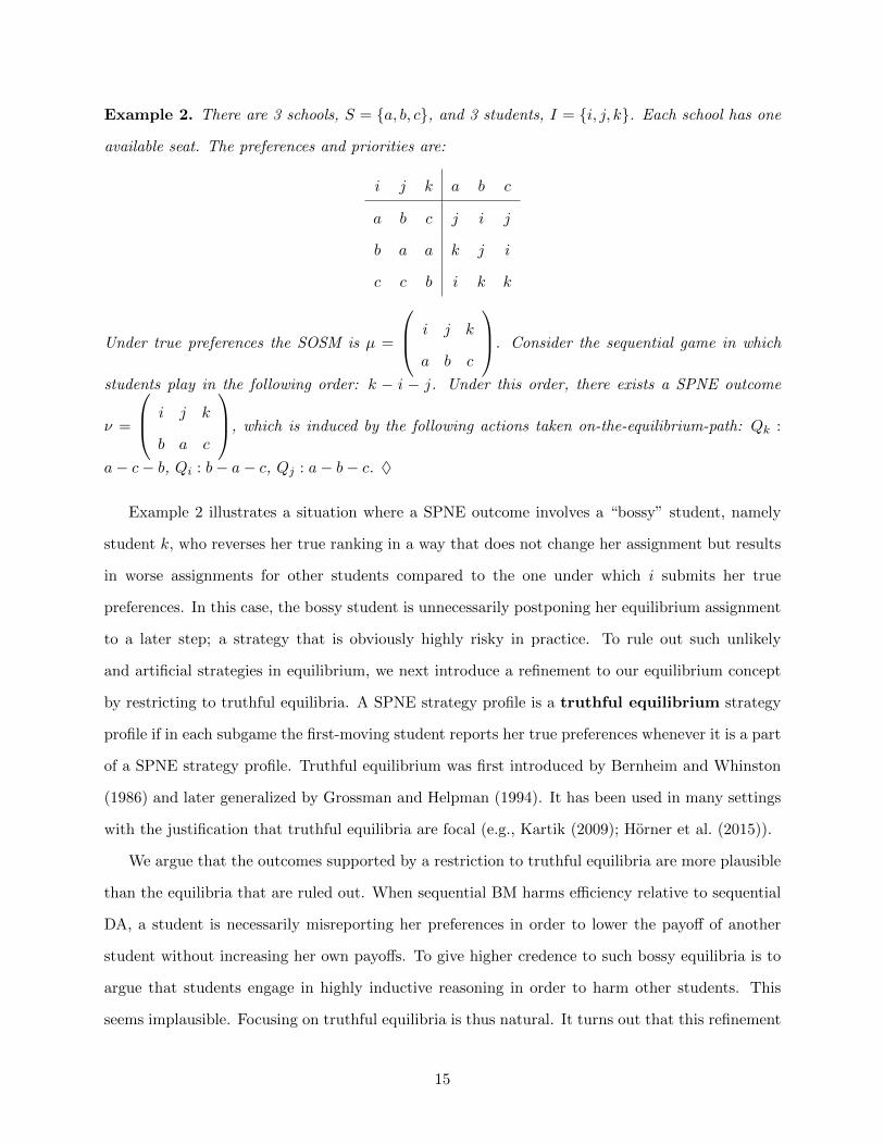
Example 2. There are 3 schools, S = a, b, c, and 3 students, I = i, j, k. Each school has one

available seat. The preferences and priorities are:

i j k a b c

a b c j i j

b a a k j i

c c b i k k

Under true preferences the SOSM is µ =

i

a

j

b

k

c

. Consider the sequential game in which

students play in the following order: k − i − j. Under this order, there exists a SPNE outcome

ν =

i

b

j

a

k

c

, which is induced by the following actions taken on-the-equilibrium-path: Qk :

a− c− b, Qi : b− a− c, Qj : a− b− c. ♦

Example 2 illustrates a situation where a SPNE outcome involves a “bossy” student, namely

student k, who reverses her true ranking in a way that does not change her assignment but results

in worse assignments for other students compared to the one under which i submits her true

preferences. In this case, the bossy student is unnecessarily postponing her equilibrium assignment

to a later step; a strategy that is obviously highly risky in practice. To rule out such unlikely

and artificial strategies in equilibrium, we next introduce a refinement to our equilibrium concept

by restricting to truthful equilibria. A SPNE strategy profile is a truthful equilibrium strategy

profile if in each subgame the first-moving student reports her true preferences whenever it is a part

of a SPNE strategy profile. Truthful equilibrium was first introduced by Bernheim and Whinston

(1986) and later generalized by Grossman and Helpman (1994). It has been used in many settings

with the justification that truthful equilibria are focal (e.g., Kartik (2009); Horner et al. (2015)).

We argue that the outcomes supported by a restriction to truthful equilibria are more plausible

than the equilibria that are ruled out. When sequential BM harms efficiency relative to sequential

DA, a student is necessarily misreporting her preferences in order to lower the payoff of another

student without increasing her own payoffs. To give higher credence to such bossy equilibria is to

argue that students engage in highly inductive reasoning in order to harm other students. This

seems implausible. Focusing on truthful equilibria is thus natural. It turns out that this refinement

15

leads to a unique equilibrium prediction that can improve upon the outcome of DA, implemented

either sequentially or simultaneously.

Proposition 3. For any problem P and any order ω, under the sequential BM game

• there exists a unique truthful equilibrium outcome, and

• it (weakly) Pareto dominates the SOSM under P .

Proof. Consider an arbitrary problem P and order ω. By the proof of Proposition 2, if DAω1(P ) is

an overdemanded school, then in any SPNE strategy profile ω1 ranks DAω1(P ) as the first choice.

Otherwise, reporting her true preferences Pω1 is a part of a SPNE strategy profile. Let Q1 be such an

equilibrium strategy for ω1. That is, if DAω1(P ) is overdemanded, then DAω1(P ) is the top choice

under Q1. Otherwise, Q1 = Pω1 . In both cases, DAi(Q1, Pω1)RiDAi(P ) for all students i ∈ I. We

can follow the same reasoning for the remaining students and obtain the desired result.

With sequential DA, it is easy to see that any truthful equilibrium outcome is equivalent to the

SOSM, which gives us the following corollary.

Corollary 2. For any problem P and order ω, the unique truthful equilibrium outcome under

the sequential BM game (weakly) Pareto dominates the unique truthful equilibrium outcome under

sequential DA.

Example 2 shows that some SPNE outcomes might be worse than the SOSM. One can wonder

whether some SPNE outcomes might be even worse than all stable outcomes. In the following

proposition, under any order and problem, we show that any SPNE outcome is weakly better than

the student pessimal stable matching under true preferences.

Proposition 4. Consider an arbitrary problem P . Let ω ∈ Ω be an arbitrary order. Given order ω,

under the sequential BM game, any SPNE outcome (weakly) Pareto dominates the student pessimal

stable matching under true preferences.

Proof. Let ν be the student pessimal stable matching under problem P . Let m be a SPNE strategy

profile and µ = BM(a(m)). With slight abuse of notation, let ak be the action played by student θk

under a(m) and ak be the action obtained from ak by truncating from the top choice (i.e., reporting

16

only the top choice under ak as acceptable). It is worth mentioning for any problem, the outcome

of the school proposing DA (sDA) mechanism is the student pessimal stable matching under that

problem.

We prove the desired result by considering students according to θ, starting with student θ1.

By Lemma 1, student θ1 is assigned to her match under DA(P ). Hence, µ(θ1)Rθ1ν(θ1). If θ1 ranks a

school weakly better than µ(θ1), then Lemma 1 implies that µ(θ1) = DAθ2(a1, P−θ1)Rθ2DAθ2(P )Rθ2ν(θ1).

Otherwise, by Lemma 1, DAθ1(a1, P−θ1) = ∅. The Rural Hospital Theorem (Roth, 1986) implies

that θ1 is unassigned under the student pessimal stable matching of the problem (a1, P−θ1). Since

sDA is individually rational and non-bossy (Afacan and Dur, 2017), sDA(a1, P−θ1) = sDA(a, P−θ1),

where ∅ is the top choice under a. Then, one can easily show that sDAj(a, P−θ1)RjsDAj(P ) for

any j ∈ I \ θ1. By Lemma 1, µ(θ2) = DAθ2(a, P−θ1)Rθ2sDAθ2(a, P−θ1)Rθ2sDAθ2(P ).

We can show the desired result by following the same reasoning for the remaining students.

3.1 Restricted Environments

We discuss two environments for which sequential BM weakly Pareto dominates any stable

outcome under true preferences in equilibrium without any refinement. First, we restrict attention

to single-choice mechanisms that impose a hard constraint on a student’s action space. With single-

choice mechanisms, students are allowed to rank at most one school in their submitted preferences.13

Proposition 5. For any problem P and order ω, under the restriction to single-choice mechanisms,

let m be a SPNE strategy profile such that under ai(m) the first ranked school is not unacceptable

for any i ∈ I. Then, BM(a(m)) (weakly) Pareto dominates the SOSM under P .

Proof. Consider a problem P and an order ω. Let µ be the SOSM under P , i.e., DA(P ) =

µ. Under our restriction to single-choice mechanisms, for each k ∈ 1, 2, . . . , |I|, student ik’s

action (message) space coincides with the preference orders over the schools and being unassigned

such that being unassigned is ranked either as the first choice or the second choice. This simply

says that each student may rank at most one school. First, by Proposition 2, existence of a

SPNE outcome that (weakly) Pareto dominates µ is guaranteed. Without loss of generality, let

ik = ωk, i.e., ik plays in step k. By Lemma 1 under any SPNE of sequential BM i1 is assigned

13 Restricting the action space has been done in several related matching papers (e.g., Bonkoungou (2016)).

17

to µ(i1). If µ(i1) 6= ∅, then in any SPNE strategy profile i1 ranks µ(i1) first. If µ(i1) = ∅,

then under our restriction to single-choice mechanisms, under m i1 ranks an acceptable school

first. Under both case, DAi2(ai1(m), P−i1)Ri2µ(i2). Hence, Lemma 1 implies that BMi2(a(m)) =

DAi2(ai1(m), P−i1)Ri2µ(i2). By using the same arguments, we can show that BMi(a(m))Riµ(i)

for all i ∈ I. This completes the proof.

Second, we consider overdemanded environments where it is not possible to assign all students

to a (real) school at the same time. In particular, we assume each student considers all schools

acceptable and the number of students is more than the number of available seats, i.e., |I| >∑s∈S qs. An overdemanded environment is consistent with many empirically relevant settings,

including elite exam schools and the magnet school environment of WCPSS that is analyzed in the

field data of the next section.14

Proposition 6. In an overdemanded environment, for any problem P , there exists an order ω such

that all SPNE outcomes of the sequential BM game Pareto dominate the SOSM under P .

Proof. Let µ be the student optimal stable matching under P , i.e., DA(P ) = µ. Assume that each

student i considers all schools acceptable and the number of students is more than the number

of available seats. In any such problem, some of the students are unassigned and all schools are

overdemanded. Let U be the set of unassigned students under µ, i.e., µ(i) = ∅ for all i ∈ U . Let

ω be an order in which each student i ∈ I \ U plays before each j ∈ U . Then, Lemma 1 and

Proposition 5 imply the desired result.

We next ask the following question: for any given problem, does there exist an order of play

that induces a SPNE outcome that is Pareto efficient? The answer to this question is affirmative

and follows from the consent idea of Kesten (2010) and Lemma 1.

Proposition 7. For any problem P , there exists an order ω such that the SPNE outcome of the

sequential BM game is Pareto efficient.

14In Wake County, around 6,000 students submit applications for less than 4,000 seats and more than 90% of theschools are overdemanded.

18

Proof. For any problem if we allow the students assigned to the underdemanded schools to play

first and play their related DA outcome as first choice we can construct a SPNE strategy profile;

by Kesten (2010) the related SPNE outcome is Pareto efficient.

4 Nonequilibrium Convergence under Myopic Best Responding

Thus far through an equilibrium analysis, we have demonstrated that sequential BM can im-

prove upon the one-shot implementation of BM. We now consider the robustness of this finding

when students are “short-sighted” and do not necessarily engage in equilibrium play, but rather

myopically best respond to the current situation when it is their turn to play. This approach is

reminiscent of the random paths to stability approach pioneered by Roth and Vate (1991).15 To

this end we consider an environment in which students can update their preferences as many times

as they want and there is no predetermined order in which students update. In this environment,

we assume that when a student updates her preferences, she can observe the last submitted pre-

ferences of each student, and in order to best respond, she ranks her best achievable school when

BM is applied to the last updated preference profile. The process of best responding terminates

when no student needs to update her submitted preferences to improve her assignment; the final

outcome is obtained by running BM. We show that for any problem, irrespective of the order of

play, this dynamic game always converges to a unique outcome, which is equivalent to the SOSM.

Proposition 8. For any problem P , if students best respond following our assumption above, then

the outcome of the dynamic BM game is the SOSM under P .

Proof. Let µ be the SOSM for problem P . Without loss of generality, we name each instance when

a student updates her preferences as a round. Let it be the student who updates her preferences in

round t. Since each student can update her preferences more than once, it is possible that it = it′

and t 6= t′. Let It = ∪t′<tit′ and Pt be the last submitted preferences of students in It for any t.

By using induction, we show that for any t, student it can achieve a school weakly better than

µ(it) (according to her true preferences) when she updates her preferences at round t. Hence, it

ranks a school weakly better than µ(it) as her top choice when she updates her preferences at round

15For subsequent studies of this approach in various types of problems, see Diamantoudi et al. (2004), Kojima andUnver (2014), and Klaus and Payot (2013).

19

t.

We start with student i1. By definition, i1 is the first player and she can get her top choice

under her true preferences by ranking it first under the submitted list. Hence, she can get a weakly

better school than µ(i1) when she submits her preferences in round 1.

Suppose up until round t each student it′ can get a school weakly better than µ(it′) when she

updates her preferences in round t′, where t′ < t . Hence, in round t student it can see that under

Pt the students who rank µ(it) as their top choices are the ones who weakly prefer µ(it) to their

assignment under µ. That is, under Pt the number of students in It \ it ranking µ(it) as their

top choices and having higher priority than it is strictly less than qµ(it). Therefore, it can achieve

either µ(it) or a school better than µ(it).

Induction also shows that, when the updating procedure terminates, there does not exist a

student-school pair (i, s) such that i prefers s to her match when the procedure terminates and

either s has unfilled seats or some student with lower priority than i is matched to s under this

procedure. This observation follows from the fact that i can update her preferences by ranking s

as her top choice and be better off.

Hence, the final assignment under dynamic BM is stable under true preferences and every

student weakly prefers her dynamic BM assignment to her assignment under the SOSM. Since

preferences are strict, this implies that the final matching is the SOSM.

Differently than with sequential BM, this “dynamic” version of BM produces a unique equili-

brium, which is the SOSM. Under our restriction to truthful equilibria, DA produces the SOSM

as its unique equilibrium. Thus, we find that dynamic BM cannot Pareto improve upon DA but

does no worse. This is in stark contrast to the result of Ergin and Sonmez (2006), which says that

simultaneous BM cannot Pareto improve upon DA but might do worse.

Our interpretation of the theoretical analysis thus far is as follows: (1) BM will not harm

efficiency with respect to DA (with a fully dynamic game) and (2) BM may Pareto improve upon

DA (when the final round of preference submissions is sequential). To evaluate whether we should

expect efficiency improvements with BM in practice, we now analyze data from a school district

that implemented BM in a way that we will argue is consistent with our sequential model.

20

5 Evidence from the Field

We now present evidence on the performance of sequential BM in practice. Our setting is the

Wake County Public School System (WCPSS) in North Carolina, which is the 15th largest district

in the nation with nearly 160,000 students. Our data are from 2014, when assignments were being

made for the 2014-2015 academic year. At this time, there were 170 schools in the system, including

38 magnet schools, which are partially-choice-based assignment schools aimed at “reduc[ing] high

concentrations of poverty and support[ing] diverse populations.”16 This is an interesting setting to

study because of the school district’s size and its diversity in terms of race/ethnicity and urbanicity.

Students in WCPSS are assigned to a base school and can apply for reassignment through the

magnet-school application process. Assignment of a student’s base school is determined by an

optimization algorithm, which is not choice based. Magnet seats are assigned (up to a school’s

capacity of magnet seats) using students’ submitted lists of preferences over schools and students’

priority points. Students submit their preferences in an application website during a two-week

application period. Students can change their ranking at any point during the two-week period.

Figure 1 shows a screenshot of the list of schools available to a given student, along with several

other pieces of information, including the magnet program(s) available at the school (programs

such as Gifted and Talented, International Baccalaureate, and Language Immersion).

An important component of the application website is that students are prominently shown the

number of “Current 1st Choice Applicants” (as shown in Figure 1). As a result, a student can

log into the application website multiple times to observe the change in relative demand for each

school. Dur et al. (2017) use these data to show that a student’s number of logins reflects her level

of strategic sophistication. They show that multiple-login students are 15.1% more likely to receive

a magnet assignment, relative to single-login students. The authors take this as evidence that

multiple-login students are responding to their admission probabilities, while single-login students

are not. This result is consistent with the sophisticated/sincere distinction of Pathak and Sonmez

(2008), where sophisticated students strategize and sincere students submit their true preferences.

Figure 2 shows the number of students whose last visit occurred on each day of the application

period. Of the 3,790 students, more than 1,000 visited on the first day of the application period

16See http://www.wcpss.net/magnet.

21

and did not visit the website again. Further, the last visit of between 300-400 students occurred on

the second, second-to-last, and last day. This pattern of visits suggests that preference submission

in WCPSS follows a sequential game, rather than a fully dynamic game where all students wait

until the end of the application period to submit preferences. That is, the field implementation of

BM is consistent with our main analysis of sequential BM but not with the dynamic BM analysis

in Section 4. As a result, we expect that an BM implementation similar to that of WCPSS has the

potential to improve efficiency with respect to a counterfactual implementation of DA.

Since we do not have field data on a counterfactual implementation of DA, we analyze our

field data with respect to how students submit preferences under sequential BM. Our goal in this

section is to understand whether students in the WCPSS implementation of sequential BM behave

in ways that are consistent with our theoretical analysis. To do so, we use data on each student’s

rank-ordered list of schools that she entered upon first visiting the application website as well as

any changes made upon additional visits (switches). Observing switches gives information that

is necessarily incomplete because we only see who switched, not who considered switching. The

framework of Pathak and Sonmez (2008) says that sophisticated (sincere) students consider (do not

consider) their admission probabilities in their ranking behavior. In this framework, observing that

a sophisticated student does not switch suggests that the number of current first-choice applicants

implies to her that her current ranking remains optimal.

In these data, only 130 students switch their rankings during the application period, relative to

3,790 total students. See Dur et al. (2017) for full details on the sample construction. Our analysis

considers current demand of students’ first choice schools over the course of the application period.

Current demand is measured as the number of students with the school listed as their first choice

at the moment of the student’s submission, relative to the school’s capacity (i.e., an overdemanded

ratio, where two implies two current first-choice applicants per seat). Current demand naturally

grows over time as more students submit preferences. There are two measures of current demand:

initial and final. Initial current demand includes only switchers and refers to the initial first-choice

school from which they switched. Final current demand includes all non-switchers and the final

first-choice school for switchers.

The results are in Figure 3. It shows the average current demand of students’ first-choice

schools, averaged among all students whose preference submission was on a particular day. The

22

upward trend in the current demand shown as Final is the natural rate of growth in average current

demand over the application period. The oscillation of the trend in the current demand shown as

Initial around the Final trend reflects switching behavior. In particular, a set of students switch

from a relatively overdemanded school to a less overdemanded school, which is when the Initial line

is above the Final line. Further, a set of students switch from a relatively underdemanded school

to a less underdemanded school, which is when the Initial line is below Final line.17

Figure 3 suggests that some students repeatedly visit the application website to observe the

growth in current demand of their preferred schools. Further, it suggests that some of these

repeated visitors switch their first-choice school in systematic ways that are consistent with our

theoretical analysis of sequential BM. The oscillation of the trend in Initial current demand around

the trend in Final current demand is driven by students switching when the Initial school becomes

either relatively overdemanded or relatively underdemanded. The result is that switching behavior

continually brings the overall demand into balance. We refrain from using the phrase “converge to

equilibrium” because our field data do not allow us to test for equilibrium play. Instead, we use

these field data to look for evidence that is suggestive of students playing in a way that is consistent

with our theory. Given the limitations of these field data, we now present additional evidence from

a controlled lab experiment.

6 Evidence from the Lab

To complement our analysis of field data, we also conduct a lab experiment. Subjects submit

preferences as one of several students seeking assignment.18 We use a complete information envi-

ronment, where students know the ordinal preference ranking of all students as well as priorities of

all students. Priorities are determined by walk-zone priority, which we refer to as district schools.

Each student has one district school and each school has one district student who has the highest

17This analysis is consistent with that of Dur et al. (2017) but complements that analysis because here we explicitlyincorporate the timing of students’ submissions/switches. In particular, here we use the current demand at the timeof the student’ submission; Dur et al. (2017) used only data on demand at the close of the application period.

18We conducted an earlier set of experimental sessions using a different design. The earlier results strongly supportour theoretical predictions. They are also similar to the results from the sessions shown here. Sequential BM waseconomically and statistically significantly more efficient than sequential DA in the environment/problem used in ourearlier sessions. After analyzing the data and presenting these results, we concluded that students were frequentlyassigned to their district school under sequential DA, but they were often able to do better than their district schoolunder sequential BM. We conducted additional sessions to ensure a robust set of comparisons. We do not pool thedata for analysis because the design changed in several ways. We point out these differences in what follows.

23

priority at the school. Ties among non-district students are broken by a fair lottery.

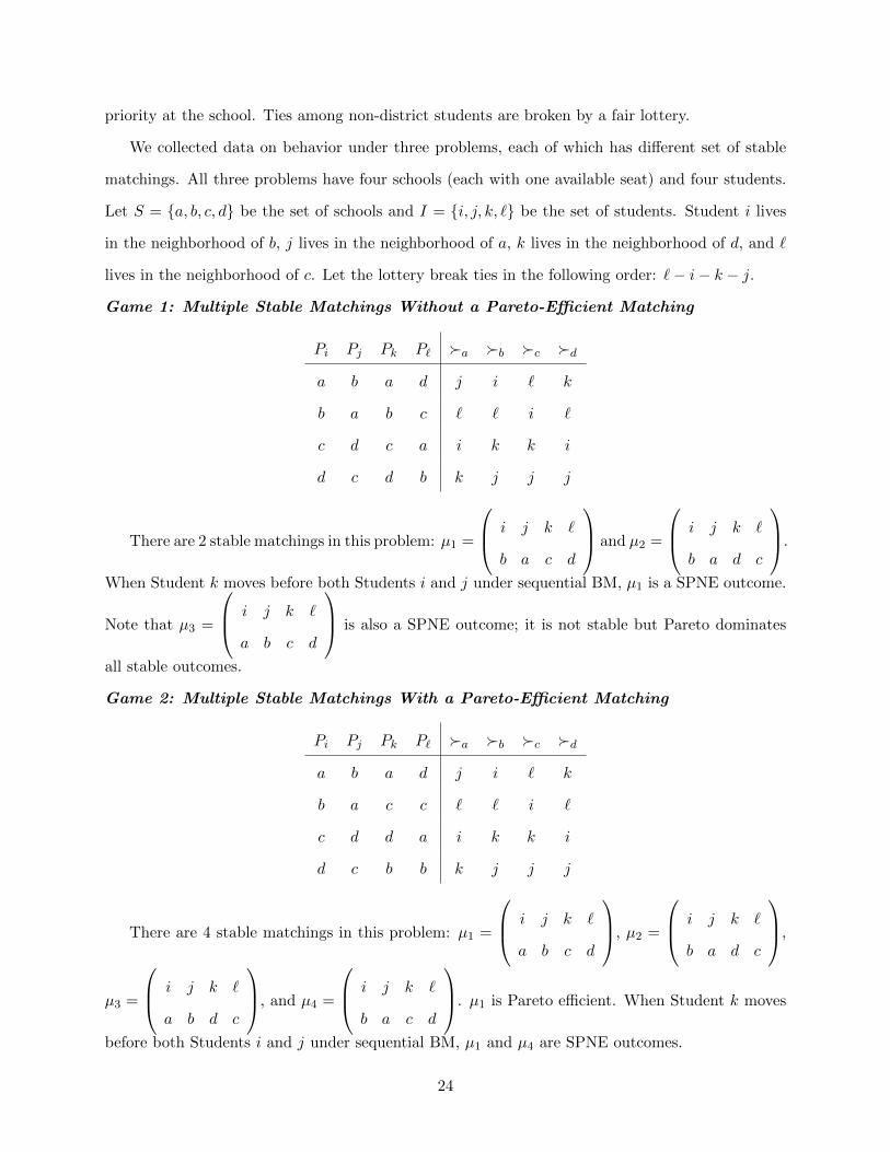
We collected data on behavior under three problems, each of which has different set of stable

matchings. All three problems have four schools (each with one available seat) and four students.

Let S = a, b, c, d be the set of schools and I = i, j, k, ` be the set of students. Student i lives

in the neighborhood of b, j lives in the neighborhood of a, k lives in the neighborhood of d, and `

lives in the neighborhood of c. Let the lottery break ties in the following order: `− i− k − j.

Game 1: Multiple Stable Matchings Without a Pareto-Efficient Matching

Pi Pj Pk P` a b c d

a b a d j i ` k

b a b c ` ` i `

c d c a i k k i

d c d b k j j j

There are 2 stable matchings in this problem: µ1 =

i

b

j

a

k `

c d

and µ2 =

i

b

j

a

k `

d c

.

When Student k moves before both Students i and j under sequential BM, µ1 is a SPNE outcome.

Note that µ3 =

i

a

j

b

k `

c d

is also a SPNE outcome; it is not stable but Pareto dominates

all stable outcomes.

Game 2: Multiple Stable Matchings With a Pareto-Efficient Matching

Pi Pj Pk P` a b c d

a b a d j i ` k

b a c c ` ` i `

c d d a i k k i

d c b b k j j j

There are 4 stable matchings in this problem: µ1 =

i

a

j

b

k `

c d

, µ2 =

i

b

j

a

k `

d c

,

µ3 =

i

a

j

b

k `

d c

, and µ4 =

i

b

j

a

k `

c d

. µ1 is Pareto efficient. When Student k moves

before both Students i and j under sequential BM, µ1 and µ4 are SPNE outcomes.

24

Game 3: Unique Pareto-Inefficient Stable Matching

Pi Pj Pk P` a b c d

a b a d j i ` k

b a b c ` ` i `

c d d a i k k i

d c c b k j j j

There is one stable matching in this problem: µ1 =

i

b

j

a

k `

d c

, which is Pareto inefficient.

When Student k moves before both Students i and j under sequential BM, µ1 is a SPNE outcome.

Note that µ3 =

i

a

j

b

k `

d c

is also a SPNE outcome; it is not stable but Pareto dominates all

stable outcomes.

These three problems are exactly the same except for the ordinal preference ranking of Student

k. We vary the set of stables matchings by changing only one aspect of the problem. Any differences

in behavior in these three problems is a clear result of the different strategic environments. Game

1 is the most interesting from a strategic perspective and is the main environment we sought to

study. We included Games 2 and 3 to check robustness.19

6.1 Experimental Sessions

We ran the experiment using zTree (Fischbacher, 2007) at the experimental lab at North Caro-

lina State University in February and March of 2017. 80 students participated in the experiment,

which lasted less than two hours. We use a two-by-two-by-three design, with treatment variation in

mechanism (BM or DA), move structure (sequential or simultaneous preference submission), and

problem (Game 1, 2, or 3). Students participated in one mechanism (between-subjects design) and

one problem (between-subjects design) but both move structures (within-subjects design). The

order of the move structures was randomized across groups such that half of students submitted

preferences sequentially first and half submitted simultaneously first (ABBA/BAAB design). The

19The earlier sessions of the experiment used incomplete information in a design that followed Dur et al. (2016).Because our results are similar in a design with incomplete information and in one with complete information, weconclude that complete information is not driving our empirical results.

25

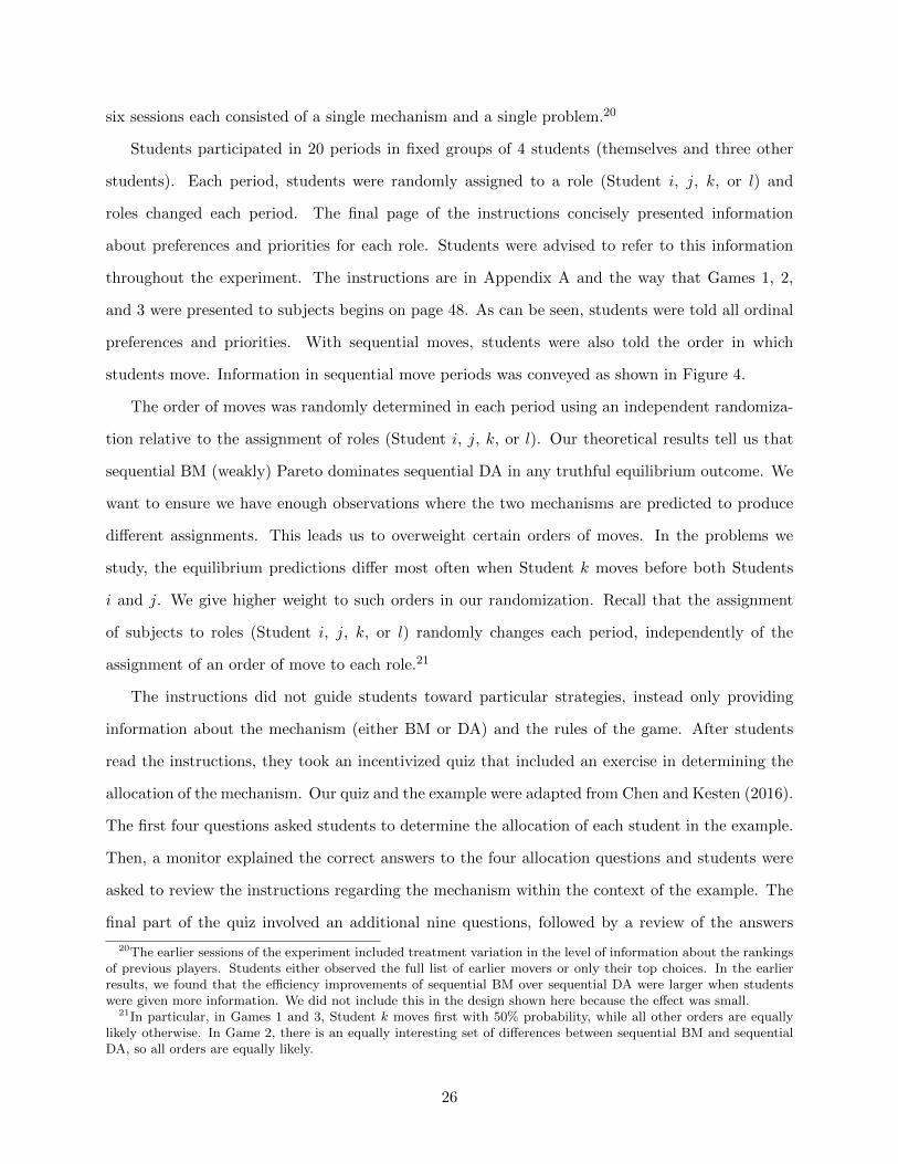
six sessions each consisted of a single mechanism and a single problem.20

Students participated in 20 periods in fixed groups of 4 students (themselves and three other

students). Each period, students were randomly assigned to a role (Student i, j, k, or l) and

roles changed each period. The final page of the instructions concisely presented information

about preferences and priorities for each role. Students were advised to refer to this information

throughout the experiment. The instructions are in Appendix A and the way that Games 1, 2,

and 3 were presented to subjects begins on page 48. As can be seen, students were told all ordinal

preferences and priorities. With sequential moves, students were also told the order in which

students move. Information in sequential move periods was conveyed as shown in Figure 4.

The order of moves was randomly determined in each period using an independent randomiza-

tion relative to the assignment of roles (Student i, j, k, or l). Our theoretical results tell us that

sequential BM (weakly) Pareto dominates sequential DA in any truthful equilibrium outcome. We

want to ensure we have enough observations where the two mechanisms are predicted to produce

different assignments. This leads us to overweight certain orders of moves. In the problems we

study, the equilibrium predictions differ most often when Student k moves before both Students

i and j. We give higher weight to such orders in our randomization. Recall that the assignment

of subjects to roles (Student i, j, k, or l) randomly changes each period, independently of the

assignment of an order of move to each role.21

The instructions did not guide students toward particular strategies, instead only providing

information about the mechanism (either BM or DA) and the rules of the game. After students

read the instructions, they took an incentivized quiz that included an exercise in determining the

allocation of the mechanism. Our quiz and the example were adapted from Chen and Kesten (2016).

The first four questions asked students to determine the allocation of each student in the example.

Then, a monitor explained the correct answers to the four allocation questions and students were

asked to review the instructions regarding the mechanism within the context of the example. The

final part of the quiz involved an additional nine questions, followed by a review of the answers

20The earlier sessions of the experiment included treatment variation in the level of information about the rankingsof previous players. Students either observed the full list of earlier movers or only their top choices. In the earlierresults, we found that the efficiency improvements of sequential BM over sequential DA were larger when studentswere given more information. We did not include this in the design shown here because the effect was small.

21In particular, in Games 1 and 3, Student k moves first with 50% probability, while all other orders are equallylikely otherwise. In Game 2, there is an equally interesting set of differences between sequential BM and sequentialDA, so all orders are equally likely.

26

by the monitor; students were encouraged to raise their hands with any final questions before the

experiment began. Students were told that they must repeat the quiz (with no earnings on the

retake) if they answer less than 10 questions correct on the quiz. The majority of students answered

12 or 13 (of 13) questions correctly and only one student failed to answer at least the required 10

questions correct. All results are robust to excluding this single student.

Before the experiment began, students were asked to enter their student ID number. In the

recruitment, students were told that they would provide their student ID number and that the

experimental data would be matched to data from their registration and enrollment records in

order to see whether “such things as GPA, academic major, etc. can enhance the predictive power

of standard economic models typically used to analyze the data.” Next, the experiment began and

students participated in 20 experimental periods. After the experiment ended, students participated

in an incentivized elicitation of their risk and ambiguity preferences, following the multiple-price

list approach of Holt and Laury (2002).

The risk elicitation came first for all students and presented a list of 10 paired choices between a

50/50 lottery and a sure payoff whose value varied around the expected value of the lottery. Finally,

the ambiguity elicitation presented students the same list of choices with the same values for the

sure payoff, where the only change is that the lottery had uncertain probabilities. Risk averse

students require a lower sure payoff to switch from the lottery, while ambiguity averse students

switch from the lottery to the sure payoff at a lower value of the sure payoff relative to the same

student’s switching point in the risk elicitation. Students made 10 choices for each elicitation (20

in total) and one was chosen at random for payment for each elicitation (two in total).

Payoffs were expressed to students as points and they were told that each point was worth $1.

Students were paid for one randomly chosen period. Earnings in dollars were $27.77 on average,

with a range of $12.75 and $38.25. These numbers include a $5 show-up fee and payments from the

quiz and each elicitation. Earnings from the experiment itself were $14.41 on average, with a range

of $0.00 and $20.00. Earnings from the quiz were $3.14 on average, relative to a maximum possible

quiz earnings of $3.25. Finally, earnings from the risk and ambiguity elicitations were $2.70 and

$2.52 on average, respectively. Each student’s cardinal preferences were always drawn such that

the school with the highest payoff was valued at 20 points, the lowest payoff at 0 points, and the

payoffs in between valued at uniformly distributed integers.

27

6.2 Experimental Results

In the results that follow, all comparisons are made using nonparametric tests (Wilcoxon rank-

sum tests in our case). To see if BM can improve efficiency relative to DA when preferences are

submitted sequentially, we use two efficiency measures. First, the assigned rank variable equals one

if the student is assigned to her most preferred school, . . ., and four if the student is assigned to

her least preferred school. Second, earnings per period equal 20 if the student is assigned to her

most preferred school, . . ., and 0 if the student is assigned to her least preferred school. As such,

these results should convey the same message, with the more efficiency mechanism generating lower

assigned rank and higher earnings per period.

Result 1. Efficiency is higher under BM than DA. The efficiency increase is statistically significant

with sequential moves but is smaller and statistically insignificant with simultaneous moves.

We measure efficiency with assigned rank in Table 1 and earnings per period in Table 2. Sequen-

tial BM assigns students to a school that is 0.14 positions higher in their ordinal preferences relative

to sequential DA (lower numbers imply more preferred school). Simultaneous BM appears to be

more efficient than simultaneous DA but the difference is smaller and not statistically significant.

We will return to the comparison of sequential and simultaneous moves in the next result.

Note that we reach the exact same conclusions in Tables 1 and 2. This is unsurprising because

being assigned to a better school according to your true preferences necessarily gives you higher

earnings. As a result, we proceed with an analysis of assigned rank only. Before moving on, we

note that earnings per period has a nice interpretation for the magnitude of the effect: sequential

BM is associated with one more dollar in earnings than sequential DA. The effect size on earnings

is quite similar to the effect size on assigned rank (0.14/1.94 = 7.1% versus 1.00/13.34 = 7.5%).22

Our next analysis separately considers students in each role (Student i, j, k, or l). Tables 1

and 2 show efficiency improvements on average but we are more interested in Pareto improvements

(more efficient allocations of some students and no less efficient allocation of any student).

Result 2. Sequential BM Pareto improves sequential DA. Simultaneous BM and simultaneous DA

22In the earlier sessions of the experiment whose results are not shown, the effect size of the efficiency gain forsequential BM over sequential DA is slightly larger: sequential BM raises efficiency by 9.9%. Specifically, assigned rankis 2.44 with sequential BM and 2.69 with sequential DA, where the difference is statistically significant (Z-statistic= 3.99, p-value = 0.00).

28

are not Pareto rankable.

Table 3 shows that average efficiency masks features that are important for a Pareto comparison.

With sequential moves, BM improves efficiency for students in every role (i, j, k, or l); these

differences are large for all students except Student j. With simultaneous moves, BM is associated

with higher efficiency for Students k and l but lower efficiency for Students i and j. This is

exactly what our theoretical results predict: BM results in miscoordination but these coordination

problems can be solved with sequential preference submission. With simultaneous BM, Student

k is sometimes able to improve her assignment at the expense of i and j. This results in less

competition for Student l’s most preferred school and she is almost always able to be seated there.

To supplement our main result that BM Pareto improves DA but only with sequential moves,

we study the three problems separately. Tables 4, 5, and 6 present the results for Games 1, 2, and 3,

respectively. Recall that Game 1 is the most interesting from a strategic perspective because it has

multiple stable matchings, none of which are Pareto efficient. Game 2 tells us how BM performs in

a situation where a Pareto efficient stable matching exists with DA (i.e., we might expect that BM

cannot do better than DA in terms of efficiency in Game 2 but might do worse). Finally, Game 3

has a unique stable matching but BM might be able to improve efficiency despite this.

Result 3. Sequential BM Pareto improves sequential DA when DA is inefficient. Sequential BM

does not have statistically significantly lower efficiency when DA is efficient.

In Table 4 for Game 1, sequential BM Pareto improves sequential DA, while simultaneous BM

is slightly but statistically insignificantly worse in terms of efficiency relative to simultaneous DA.

In Table 5 for Game 2, we know theoretically that BM cannot improve efficiency relative to DA.

The results show that students in each role do worse with sequential BM relative to sequential

DA; the differences are meaningful in size but statistically insignificant. With simultaneous moves,

BM results in miscoordination that completely offsets from the point of view of average efficiency.

Finally, in Table 6 for Game 3, the comparison of BM to DA appears similar in terms of average

efficiency but there are large efficiency tradeoffs with simultaneous moves. With sequential moves,

the main efficiency difference between BM and DA is a large efficiency improvement of BM for

Student l that is not offset to a statistically significant degree for any other student. This is again

consistent with a Pareto ranking of sequential BM over sequential DA.

29

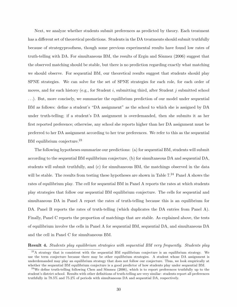
Next, we analyze whether students submit preferences as predicted by theory. Each treatment

has a different set of theoretical predictions. Students in the DA treatments should submit truthfully

because of strategyproofness, though some previous experimental results have found low rates of

truth-telling with DA. For simultaneous BM, the results of Ergin and Sonmez (2006) suggest that

the observed matching should be stable, but there is no prediction regarding exactly what matching

we should observe. For sequential BM, our theoretical results suggest that students should play

SPNE strategies. We can solve for the set of SPNE strategies for each role, for each order of

moves, and for each history (e.g., for Student i, submitting third, after Student j submitted school

. . .). But, more concisely, we summarize the equilibrium prediction of our model under sequential

BM as follows: define a student’s “DA assignment” as the school to which she is assigned by DA

under truth-telling; if a student’s DA assignment is overdemanded, then she submits it as her

first reported preference; otherwise, any school she reports higher than her DA assignment must be

preferred to her DA assignment according to her true preferences. We refer to this as the sequential

BM equilibrium conjecture.23

The following hypotheses summarize our predictions: (a) for sequential BM, students will submit

according to the sequential BM equilibrium conjecture, (b) for simultaneous DA and sequential DA,

students will submit truthfully, and (c) for simultaneous BM, the matchings observed in the data

will be stable. The results from testing these hypotheses are shown in Table 7.24 Panel A shows the

rates of equilibrium play. The cell for sequential BM in Panel A reports the rates at which students

play strategies that follow our sequential BM equilibrium conjecture. The cells for sequential and

simultaneous DA in Panel A report the rates of truth-telling because this is an equilibrium for

DA. Panel B reports the rates of truth-telling (which duplicates the DA entries from Panel A).

Finally, Panel C reports the proportion of matchings that are stable. As explained above, the tests

of equilibrium involve the cells in Panel A for sequential BM, sequential DA, and simultaneous DA

and the cell in Panel C for simultaneous BM.

Result 4. Students play equilibrium strategies with sequential BM very frequently. Students play

23A strategy that is consistent with the sequential BM equilibrium conjecture is an equilibrium strategy. Weuse the term conjecture because there may be other equilibrium strategies. A student whose DA assignment isunderdemanded may play an equilibrium strategy that does not follow our conjecture. Thus, we look empirically atwhether the sequential BM equilibrium conjecture is a good predictor of how students play under sequential BM.

24We define truth-telling following Chen and Sonmez (2006), which is to report preferences truthfully up to thestudent’s district school. Results with other definitions of truth-telling are very similar: students report all preferencestruthfully in 78.5% and 75.2% of periods with simultaneous DA and sequential DA, respectively.

30

equilibrium strategies with DA (truth-telling) at rates that are also quite high. Groups reach stable

matchings frequently with simultaneous BM.

From Table 7, students play equilibrium strategies 83.8% of the time with sequential BM. This

high rate of equilibrium play provides strong support for the empirical validity of our theoretical

predictions. For further evidence, we compare the rates of equilibrium play with sequential BM

separately depending on the relative position of Student k in the move order; this allows us to see

whether students play equilibrium strategies more often when it is easier to understand that the

strategy is an equilibrium.25 In unreported results, when Student k moves before both Students i

and j, the subsequent students follow equilibrium strategies 86.6% of the time. This is statistically

significantly higher than the rate of equilibrium play when Student k moves later, which is 79.8%

(standard error of the difference = 0.04, p-value = 0.07). We conclude that students frequently

follow the sequential BM equilibrium conjecture; because students submit preferences as predicted

by our model, sequential BM generates the predicted efficiency gains.

Truth-telling rates with DA are 79.5% and 75.7% with simultaneous and sequential moves,

respectively.26 This suggests that our equilibrium conjecture with sequential BM and truth-telling

with DA are both useful predictors of how students submit preferences in the lab. Truth-telling

is shown for DA in Panel A (because it is an equilibrium strategy) and in Panel B (to compare

truth-telling with BM). As expected, truth-telling is lower with BM. When comparing DA and BM

in Panel B, recall that students are not predicted to report truthfully with BM. Panels A and B do

not provide evidence that subjects are confused with BM and simply playing truthfully or noisily.

Finally, Panel C of Table 7 reports the proportion of matchings that are stable. With simul-

taneous BM, we predict stability but do not have a prediction regarding which matching will be

observed. In these data, groups reached a stable matching in 64.0% of periods under simultaneous

BM. For either DA treatment, 84.0% of matchings are stable.27 The high rates of stability we find

25When Student k moves before both Students i and j, subsequent students can easily see whether their DAassignment is overdemanded. This makes it easier to find their equilibrium strategies. Before Student k has submittedher preferences, other students have to best respond to their beliefs regarding what she will submit. See the problemsof interest shown earlier, starting on page 24.

26These rates of truth-telling with DA are high but not inconsistent with the related experimental literature. Forexample, other papers have found truth-telling rates of 72.2% (in the “designed” environment of Chen and Sonmez(2006)), 75.1% (Chen and Kesten, 2016) , and 82.2% (in the “zero information” environment of Pais and Pinter(2008)). The treatment in Pais and Pinter (2008) that is most comparable to our environment is that of “fullinformation,” where their rate of truth-telling is 46.7%.

27These rates of stability are consistent with some findings the literature. For simultaneous DA, Klijn et al. (2013)

31

for DA are consistent with the high rates of equilibrium play. Finally, note that stability is lowest

with sequential DA at 53.0%. However, stability with sequential DA is sometimes in conflict with

efficiency. This occurs in two of the environments we tested in the lab, Games 1 and 3, in which

there exist SPNE matchings that are not stable but Pareto dominate all stable matchings.

Our final exercise looks at a specific prediction of our model to check if BM’s efficiency gains

are driven by the features that we predict to be at work. Theoretically, sequential BM is (weakly)

more efficient than sequential DA for any order in any truthful equilibrium. Further, our model

tells us exactly the situations that BM can improve efficiency relative to DA (i.e., a strict efficiency

comparison). We now look at whether the Pareto improvements we find with sequential BM are

coming when theory says they should be. For the problems we study, BM can (strictly) improve

efficiency when Student k moves before both Students i and j. Table 8 compares efficiency between

BM and DA separately for cases where Student k moves earlier than i and j relative to cases

where k moves later than either i or j. Of course, this comparison only considers sequential move

periods because simultaneous move periods do not have an order of moves to compare. To maintain

a tight link with our theoretical model, we only include periods where subjects play equilibrium

strategies. That is, we only include periods where all four students in the group played according

to the sequential BM equilibrium conjecture (for sequential BM) or truth-telling (for sequential

DA).28

Result 5. The Pareto efficiency improvement observed for sequential BM over sequential DA

happens in the cases predicted by the model: when Student k moves before both Students i and j.

Our experimental design overweighted certain orders of moves. This embedded the fact that

theory tells us that there is increased scope for (strict) efficiency improvements on DA with some

orders relative to other orders. Our theoretical results tell us that sequential BM is (weakly) more

efficient than sequential DA in general. But in the problems we study, sequential BM can (strictly)

Pareto improve upon sequential DA when Student k moves before both Students i and j. Table 8

shows that this is exactly what we find in the data. When theory says BM cannot improve upon

find that 85.0% of matchings are stable, while Pais and Pinter (2008) find 44.4% in the comparable informationenvironment (but as high as 88.9% in other treatments). For simultaneous BM, Klijn et al. (2013) find 65.0%, whilePais and Pinter (2008) find 44.4%.

28We separately present the results on efficiency by order of moves for all periods in unreported results. Theseresults also find that sequential BM is more efficient than sequential DA and that this holds in periods where efficiencygains are predicted by our theoretical model.

32

DA, sequential BM offers neither an average efficiency improvement nor a Pareto improvement over

sequential DA. In contrast, when theory says there is scope of efficiency improvements, sequential

BM does indeed Pareto improve upon sequential DA.

This supports our claims for why BM improves efficiency. While the Pareto improvement we find

for BM over DA is driven by certain orders of moves, our data suggest that BM is (weakly) more

efficient for any order. This is consistent with our theoretical results under truthful equilibria.

Therefore, a school district or college who uses sequential BM is not required to have specific

knowledge of true preferences to implement sequential BM in a way that does not harm students.

7 Conclusions

With choice-based assignment in school districts across the United States and the world, the

Boston Mechanism (BM) remains the most commonly used mechanism. Currently this mechanism

is implemented as a simultaneous-move game and is at the center of the school-choice debate.

Notably, it is not strategyproof and has poor (ex post) equilibrium outcomes from the perspective

of efficiency. However, we show that its shortcomings can be rectified once preference submissions

are organized sequentially (i.e., students are allowed to submit their preferences over time). For

example, it is not uncommon in assignment applications to allow students to have several days or

weeks over which they can submit their preferences and revise their submissions. When information

is revealed during this process, we find that students can best respond to information about other

students’ submitted preferences; this best-responding behavior might improve the performance of

the mechanism both in and out of equilibrium. Our findings have important policy implications

as they may help improve student assignments with little adjustments to current plans in places

where BM is currently in use. We find that when students apply sequentially, the coordination

problem in school assignment can be mitigated and BM does no worse than DA both theoretically

and experimentally.

33

References

Abdulkadiroglu, A., Y.-K. Che, P. A. Pathak, A. E. Roth, and O. Tercieux (2017):

“Minimizing Justified Envy in School Choice: The Design of New Orleans’ OneApp,” Tech. rep.,

National Bureau of Economic Research.

Abdulkadiroglu, A., Y.-K. Che, and Y. Yasuda (2011): “Resolving Conflicting Preferences

in School Choice: The “Boston Mechanism” Reconsidered,” American Economic Review, 399–

410.

Abdulkadiroglu, A., P. Pathak, and A. Roth (2009): “Strategyproofness versus Efficiency

in Matching with Indifferences: Redesigning the NYC High School Match,” American Economic

Review, 99, 1954–1978.

Abdulkadiroglu, A., P. A. Pathak, A. E. Roth, and T. Sonmez (2006): “Changing the

Boston School Choice Mechanism,” mimeo.

Abdulkadiroglu, A. and T. Sonmez (2003): “School Choice: A Mechanism Design Approach,”

American Economic Review, 93, 729–747.

Afacan, M. O. and U. Dur (2017): “When Preference Misreporting is Harm[less]ful?” Journal

of Mathematical Economics, 72, 16–24.

Agarwal, N. and P. Somaini (2014): “Demand Analysis Using Strategic Reports: An Applica-

tion to a School Choice Mechanism,” mimeo.

Alcalde, J., D. Perez-Castrillo, and A. Romero-Medina (1998): “Hiring Procedures to

Implement Stable Allocations,” Journal of Economic Theory, 82, 469480.

Alcalde, J. and A. Romero-Medina (2000): “Simple Mechanisms to Implement the Core of

College Admissions Problems,” Games and Economic Behavior, 31, 294–302.

Balinski, M. and T. Sonmez (1999): “A Tale of Two Mechanisms: Student Placement,” Journal

of Economic Theory, 84, 73–94.

Bando, K. (2014): “On the existence of a strictly strong Nash equilibrium under the student-

optimal deferred acceptance algorithm,” Games and Economic Behavior, 87, 269–287.

34

Bernheim, B. D. and M. D. Whinston (1986): “Menu auctions, resource allocation, and eco-

nomic influence,” Quarterly Journal of Economics, 101, 1–31.

Bo, I. and R. Hakimov (2016a): “Iterative Versus Standard Deferred Acceptance: Experimental

Evidence,” mimeo.

——— (2016b): “The Iterative Deferred Acceptance Mechanism,” mimeo.

Bonkoungou, S. (2016): “Pareto Dominance of Deferred Acceptance through Early Decision,”

mimeo.

Chen, Y. and O. Kesten (2016): “Chinese College Admissions and School Choice Reforms: An

Experimental Study,” mimeo.

——— (2017): “Chinese College Admissions and School Choice Reforms: A Theoretical Analysis,”

Journal of Political Economy, 125, 99–139.

Chen, Y. and T. Sonmez (2006): “School Choice: An Experimental Study,” Journal of Economic

Theory, 127, 202–231.

Cookson, P. W. (1995): School choice: The struggle for the soul of American education, Yale

University Press.

Diamantoudi, E., E. Miyagawa, and L. Xue (2004): “Random paths to stability in the room-

mate problem,” Games and Economic Behavior, 48, 18–28.

Dur, U., R. G. Hammond, and T. Morrill (2016): “The Secure Boston Mechanism: Theory

and Experiments,” mimeo.

——— (2017): “Identifying the Harm of Manipulable School-Choice Mechanisms,” American Eco-

nomic Journal: Economic Policy, forthcoming.

Echenique, F. and J. Oviedo (2006): “A Theory of Stability in Many to Many Matching

Markets,” Theoretical Economics, 1, 233–273.

Ergin, H. and T. Sonmez (2006): “Games of School Choice under the Boston Mechanism,”

Journal of Public Economics, 90, 215–237.

35

Fischbacher, U. (2007): “z-Tree: Zurich Toolbox for Ready-Made Economic Experiments,”

Experimental Economics, 10, 171–178.

Gale, D. and L. Shapley (1962): “College Admissions and the Stability of Marriage,” American

Mathematical Monthly, 69, 9–15.

Glenn, C. L. (1991): “Controlled Choice in Massachusetts Public Schools.” Public Interest, 103,

88–105.

Gong, B. and Y. Liang (2016): “A Dynamic College Admission Mechanism in Inner Mongolia:

Theory and Experiment,” mimeo.

Grossman, G. M. and E. Helpman (1994): “Protection for Sale,” American Economic Review,

84, 833–850.

Haeringer, G. and F. Klijn (2009): “Constrained School Choice,” Journal of Economic Theory,

1921–1947.

Holt, C. A. and S. K. Laury (2002): “Risk Aversion and Incentive Effects,” American Economic

Review, 92, 1644–1655.

Horner, J., S. Takahashi, and N. Vieille (2015): “Truthful equilibria in dynamic Bayesian

games,” Econometrica, 83, 1795–1848.

Jaramillo, P., C. Kayi, and F. Klijn (2017): “School Choice: Nash Implementation of Stable

Matchings through Rank-Priority Mechanisms,” mimeo.

Kartik, N. (2009): “Strategic communication with lying costs,” Review of Economic Studies, 76,

1359–1395.

Kesten, O. (2010): “School choice with consent,” Quarterly Journal of Economics, 125, 1297–

1348.

Kesten, O. and M. Kurino (2012): “On the (im)possibility of improving upon the student-

proposing deferred acceptance mechanism,” Tech. rep., WZB Discussion Paper.

Klaus, B. and F. Payot (2013): “Paths to stability in the assignment problem,” Cahier de

recherches conomiques du DEEP.

36

Klijn, F., J. Pais, and M. Vorsatz (2013): “Preference Intensities and Risk Aversion in School

Choice: A Laboratory Experiment,” Experimental Economics, 16, 1–22.

Klijn, F., J. Pais, M. Vorsatz, et al. (2016): “Static versus Dynamic Deferred Acceptance in

School Choice: Theory and Experiment,” mimeo.

Kojima, F. and U. Unver (2014): “The “Boston” School-Choice Mechanism: An Axiomatic

Approach,” Economic Theory, 53, 515–544.

McVitie, D. G. and L. B. Wilson (1971): “The stable marriage problem,” Communications of

the ACM, 14, 486–490.

Pais, J. and A. Pinter (2008): “School Choice and Information: An Experimental Study on

Matching Mechanisms,” Games and Economic Behavior, 64, 303–328.

Pathak, P. A. and T. Sonmez (2008): “Leveling the Playing Field: Sincere and Sophisticated

Players in the Boston Mechanism,” American Economic Review, 98, 1636–1652.

Romero-Medina, A. and M. Triossi (2014): “Non-revelation Mechanisms in Many-to-one Mar-

kets,” Games and Economic Behavior, 87, 624–630.

——— (2016): “Take-it-or-leave-it Contracts in Many-to-many Matching Markets,” mimeo.

Roth, A. E. (1986): “On the allocation of residents to rural hospitals: a general property of

two-sided matching markets,” Econometrica, 54, 425–427.

Roth, A. E. and J. H. V. Vate (1991): “Incentives in two-sided matching with random stable

mechanisms,” Economic Theory, 1, 31–44.

Sotomayor, M. (2004): “Implementation in the Many-to-Many Matching Market,” Games and

Economic Behavior, 46, 199–212.

Stephenson, D. G. (2016): “Continuous Feedback in School Choice Mechanisms,” mimeo.

Troyan, P. (2012): “Comparing school choice mechanisms by interim and ex-ante welfare,” Games

and Economic Behavior, 75, 936–947.

37

Vaznis, J. (2014): “Boston School-Assignment Letters in the Mail,” Boston Globe, March 25,

https://goo.gl/Na1Akn.

WCPSS (2015): “Wake County Public School System District Facts 2015-2016,” http://www.

wcpss.net/domain/100.

38

A Experimental Instructions

A.1 Instructions for the Boston Mechanism

Welcome!

Today you will participate in an experiment where you can earn a considerable amount of money

that will be paid to you in cash as you leave today. The following instructions tell you everything

you need to know to earn as much as possible, so please read them carefully. If you have any

questions, please raise your hand and a monitor will come and answer them.

You will play the role of a student choosing a school. You will rank schools in an application

process in order to try to get a seat at the best school you are able. You will earn points based on

how much you like the school at which you get a seat, where the number of points at a school is

called your payoff at that school. These payoffs tell you how much you like each school.

You have been randomly assigned to a group of four students (you and three other students).

The other students in the room are also in groups of four students but may be in a different group

than you are. You will not be told who else in the room is in your group and they will not be told

that you are in their group.

We will repeat the application process several times, each time called a period. In each period,

you will have a turn to rank schools. Once all students in your group have submitted their rankings,

all applications are submitted to schools in order to determine which students get admitted to which

schools.

You will participate in 20 periods in today’s experiment. After the last period, the computer

will randomly choose one period to count for your payment. Any one of the periods could be the

period that counts! Treat each period as if it is the one that determines your payment.

All points that you earn in today’s experiment will be converted to American dollars and you

will be paid in cash at the end of the experiment. Every point equals $1. Your goal is to earn as

many points as possible in order to earn as much cash as possible!

39

You will always have a copy of these instructions to refer to and you are encouraged to look

over the instructions again during the experiment.

Payoffs

There are four schools: A, B, C, and D. Each school has 1 available seat. There are 4 students

(including you) trying to gain admission to one of the schools.

Each student (you and the other students in your group) will be assigned a role for each period.

Your role is determined by your letter: I, J,K,L. Roles are randomly selected by the computer

program for each period and change from period to period. In a given period, your role determines

which school has the highest, second highest, etc. payoff for you:

Highest Payoff = 20 points2nd Highest Payoff = 10, 11, 12, 13, 14, or 15 points (each equally likely)3rd Highest Payoff = 4, 5, 6, 7, 8 or 9 points (each equally likely)

Lowest Payoff = 0 points

Being assigned to a school that gives you a higher payoff earns you more points and therefore

more cash in your pocket!

More information on the student in each role (I, J,K,L) is shown on the final page of these

instructions. Refer to this information throughout.

Application Process

At each school, you have a priority that affects the order in which your application will be

considered at that school. Your priority at each school depends on three things:

• Whether you live within the school district of that school,

• The place you rank that school in your list,

• Your order in the tie-breaking lottery.

Each school has a district student and each student has a district school; as you see above,

this affects the priority order. Your role (I, J,K,L) for the period determines which school is your

40

district school, as shown on the final page of these instructions.

The priority order of the students for each school is determined as follows:

• First Priority Level: Participants who rank the school as their first choice and live within the

school district.

• Second Priority Level: Participants who rank the school as their first choice and do not live

within the school district.

• Third Priority Level: Participants who rank the school as their second choice and live within

the school district.

• Fourth Priority Level: Participants who rank the school as their second choice and do not

live within the school district.

• · · ·

Tie Breaking

A fair lottery is used to break ties between participants at the same priority level. Your role

(I, J,K,L) in each period determines your order in the tie-breaking lottery. This is shown on the

final page of these instructions.

Steps of the Application Process

When you submit your rankings of schools, the system takes your rankings with those of the

other students in your group in order to determine which students get which seats. This process

works as follows:

• An application to the first choice school is sent for each student.

• Throughout the process, a school cannot hold more than one application. If a school recei-

ves more than one application, then it rejects the students with the lowest priorities. The

application of student with the highest priority at the school is retained.

41

• Whenever a student is rejected at a school, his/her application is sent to the next highest

(best) school on his/her list.

• Whenever a school receives new applications, these applications are considered together with

the retained applications for that school. Among the retained and new applications, the

lowest priority ones are rejected, while the application of student with the highest priority at

the school is retained.

• The process ends when all seats are taken.

• Each student is assigned to the school that holds his/her application at the end of the process.

Each period, you will have up to three minutes to submit your rankings of schools.

Game A and Game B

In today’s experiment, you will participate in two games: Game A and Game B. For half of

the periods, you will play Game A and, for the other half, you will play Game B. Every 5 periods,

the game may change from Game A to Game B, or vice versa, but you will always be told at the

beginning of each group of 5 periods which game you are about to play.

The steps of the application process, and all of the other instructions above, apply to both

games. The only thing that is different between Game A and Game B is the order in which

students submit their rankings. In Game A, students take turns, each having one turn, and the

applications are considered by schools after all students have had a turn. In Game B, all students

submit their rankings at the same time.

In both games, you will always be shown your role, which is whether you are Student I, Student

J , Student K, or Student L.

In Game A, you will also be shown the order in which you move.

Game A

In Game A, the computer program randomly selects one student in your group to go first and

the order of turns for the remaining students. The order changes from period to period. The first

42

student to have a turn is shown his/her payoff for each school as shown in the left panel below:

The second student is then shown his/her payoff for each school and is also shown the submitted

choices of the student who went first as shown in the right panel above.

Note that the payoffs are different in these two screens because the left screen shows the payoffs

of the first student and the right screen shows the payoffs of the second student.

The third and fourth students are shown their payoffs and the information about each student

who went before them (first and second mover for the third student; first, second, and third mover

for the fourth student). Once the fourth student submits his/her ranking, the period ends and all

applications are submitted to schools to determine which students get admitted to which schools.

You will be shown your assigned school, then the next period begins.

In Game A, you will always be shown the role (I, J,K,L) of the student at each position in the

order, as shown below:

43

Game B

In Game B, all students submit their rankings at the same time. Since all students submit their

rankings at the same time, no student is shown the submitted ranking of any other student.

Once all students in the room have finished reading this part of the instructions, the monitor

will review the instructions aloud and go through an example.

An Example: We will go through an example to illustrate how the application process works.

You will be asked to work out the assignments in this example for Review Question 1.

Feel free to refer to the experimental instructions before you answer any question. Each correct

answer is worth 0.25 points, which will be added to your total earnings. You can earn up to 3.25

points for the review questions.

Students and Schools: There are four students, 1-4, and four schools, A, B, C, and D.

Student ID Number: 1, 2, 3, 4; Schools: A, B, C, D

Slots and Residents: There is one slot at each school. Residents of districts are indicated in

the table below.

School District Residents

A 1

B 2

C 3

D 4

Lottery: The order in the tie-breaking lottery is as follows:

Highest Position 2nd Position 3rd Position Last Position

Student 2 Student 4 Student 1 Student 3

Submitted School Rankings: The students submit the following school rankings:

44

Student 1 Student 2 Student 3 Student 4

1st Choice D D A A

2nd Choice A A B D

3rd Choice C B C B

Last Choice B C D C

Priority: School priorities depend first on the place ranked on preference list, second on the

district resident, and last on the lottery order:

Priority order at A: 4− 3− 1− 2

Priority order at B: 3− 2− 4− 1

Priority order at C: 3− 1− 2− 4

Priority order at D: 2− 1− 4− 3

The process consists of the following steps: Please use this sheet to work out the allocation and

enter it into the computer for Review Question #1.

Step 1: Each student applies to his/her first choice. If a school receives more applications

than its capacity, then it rejects the students with the lowest priorities. The remaining students

are retained.

Applicants School Accept Hold Reject

→ A → N/A

→ B → N/A

→ C → N/A

→ D → N/A

Step 2: Each student rejected in Step 1 applies to his/her next highest (best) school. Whenever

a school receives new applications, these applications are considered together with the retained

applications for that school. Among the retained and new applications, the lowest priority ones in

excess of the school’s capacity are rejected, while remaining applications are retained.

45

Held Applicants School Accept Hold Reject

→ A → N/A

→ B → N/A

→ C → N/A

→ D → N/A

Step 3: Each student rejected in Step 2 applies to his/her next highest (best) school. Whenever

a school receives new applications, these applications are considered together with the retained

applications for that school. Among the retained and new applications, the lowest priority ones in

excess of the school’s capacity are rejected, while remaining applications are retained.

Held Applicants School Accept Hold Reject

→ A → N/A

→ B → N/A

→ C → N/A

→ D → N/A

The process ends at Step 3.

Please enter your answer to the computer for Review Question 1. Feel free to look through the

instructions and the example as you complete this and the remaining Review Questions.

Correct Answer for DA: Student 1 is allocated to School A, 2 to B, 3 to C, and 4 to D. Correct

Answer for BM: Student 1 is allocated to School C, 2 to D, 3 to B, and 4 to A.

If you have any questions, please raise your hand and a monitor will come to answer your

questions in private.

Afterward, you will be asked to answer another 9 review questions.

Review Questions 2 - 10

46

2. How many schools are available for students to be assigned in each period? Correct Answer:

4

3. True or false: In Game A, you and the other students in your group will always play in the

same order. Correct Answer: False

4. True or false: A student who lives in a school’s district and ranks the school first has higher

priority than a student who does not live in the district and ranks the school first. Correct

Answer: True

5. Suppose that Student 1’s district school is school C and Student 2’s district school is school

A. If Student 1 ranks school C second on her list and Student 2 ranks school C first on his list,

which student has a higher priority at school C? Correct Answer for DA: Student 1 Correct

Answer for BM: Student 2

6. True or false: In Game A, if you are the third student to have a turn, the first student can

change his/her submitted preferences after your turn. Correct Answer: False

7. True or false: The school that gives you the highest payoff will be the same for the entire 20

periods. Correct Answer: False

8. True or false: Roles (I, J,K,L) change from period to period. Correct Answer: True

9. True or false: In Game B, you will be shown the choices of the students who moved before

you. Correct Answer: False

10. True or false: The other students in your group may have a different favorite school than you.

Correct Answer: True

As a reminder, each correct answer is worth 0.25 points, which will be added to your total

earnings. You can earn up to 3.25 points for the review questions.

Of the 13 review questions, you need to answer at least 10 correctly in order to continue to the

experiment. If you answer fewer than 10 questions correctly, you will be asked to retake the quiz

until you correctly answer at least 10 questions. However, you will only be paid for the number of

47

questions correct on the first quiz attempt. You may ask questions at any point and may refer to

the instructions and the example throughout the quiz and the experiment itself.

If you have any questions, please raise your hand and a monitor will come to answer your

questions in private.

Information for Today’s Session [Game 1]

Students and Schools: There are four students, I, J , K, and L, and four schools, A, B, C,

and D.

Slots and Residents: There is one slot at each school. Residents of districts are indicated in

the table below.

School District Residents

A Student J

B Student I

C Student L

D Student K

Lottery: The order in the tie-breaking lottery is as follows:

Highest Position 2nd Position 3rd Position Last Position

Student L Student I Student K Student J

48

Order of Schools: The students earn the highest payoffs from schools in the following order:

Student I Student J Student K Student L

Highest Payoff A B A D

2nd Highest Payoff B A B C

3rd Highest Payoff C D C A

Lowest Payoff D C D B

[This is the end of the instructions for Game 1. For Games 2 and 3, the only difference is in

the table of ordinal preferences and only for Student k.]

Information for Today’s Session [Game 2]

· · ·

Student I Student J Student K Student L

Highest Payoff A B A D

2nd Highest Payoff B A C C

3rd Highest Payoff C D D A

Lowest Payoff D C B B

· · ·

Information for Today’s Session [Game 3]

· · ·

Student I Student J Student K Student L

Highest Payoff A B A D

2nd Highest Payoff B A B C

3rd Highest Payoff C D D A

Lowest Payoff D C C B

· · ·

49

Fig

ure

1:S

cree

nsh

otof

WC

PSS

Ap

pli

cati

onW

ebsi

te

50

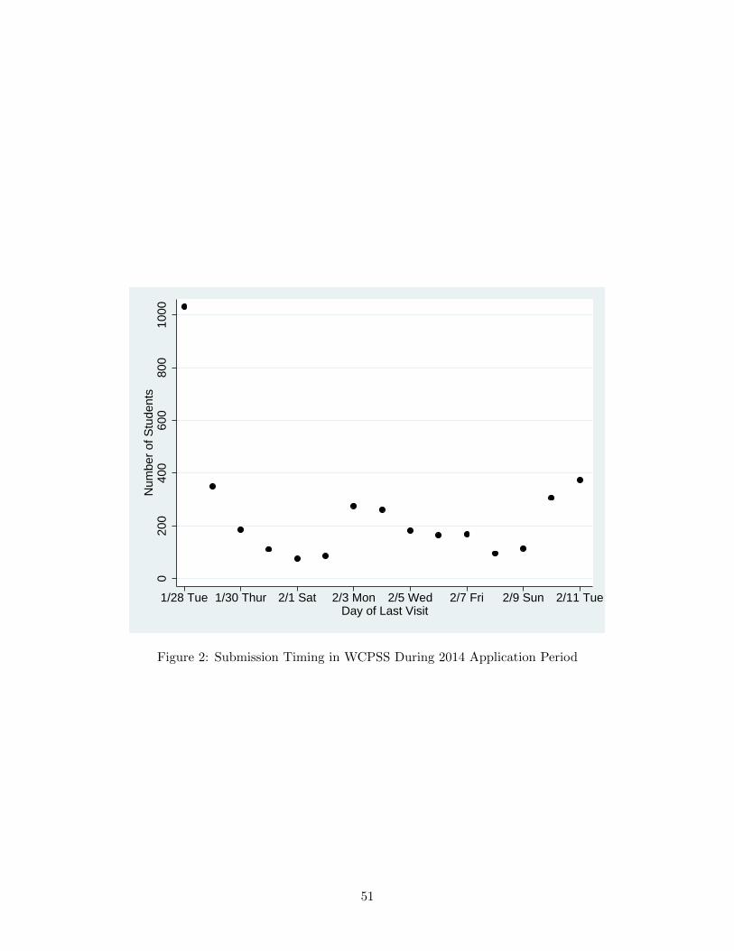
020

040

060

080

010

00N

umbe

r of

Stu

dent

s

1/28 Tue 1/30 Thur 2/1 Sat 2/3 Mon 2/5 Wed 2/7 Fri 2/9 Sun 2/11 Tue Day of Last Visit

Figure 2: Submission Timing in WCPSS During 2014 Application Period

51

0.5

11.

52

Cur

rent

Dem

and

1/28 Tue 1/30 Thur 2/1 Sat 2/3 Mon 2/5 Wed 2/7 Fri 2/9 Sun 2/11 Tue Day of Submission

Initial Final

Figure 3: Growth in Demand of First-Choice Schools and Ranking Changes

52

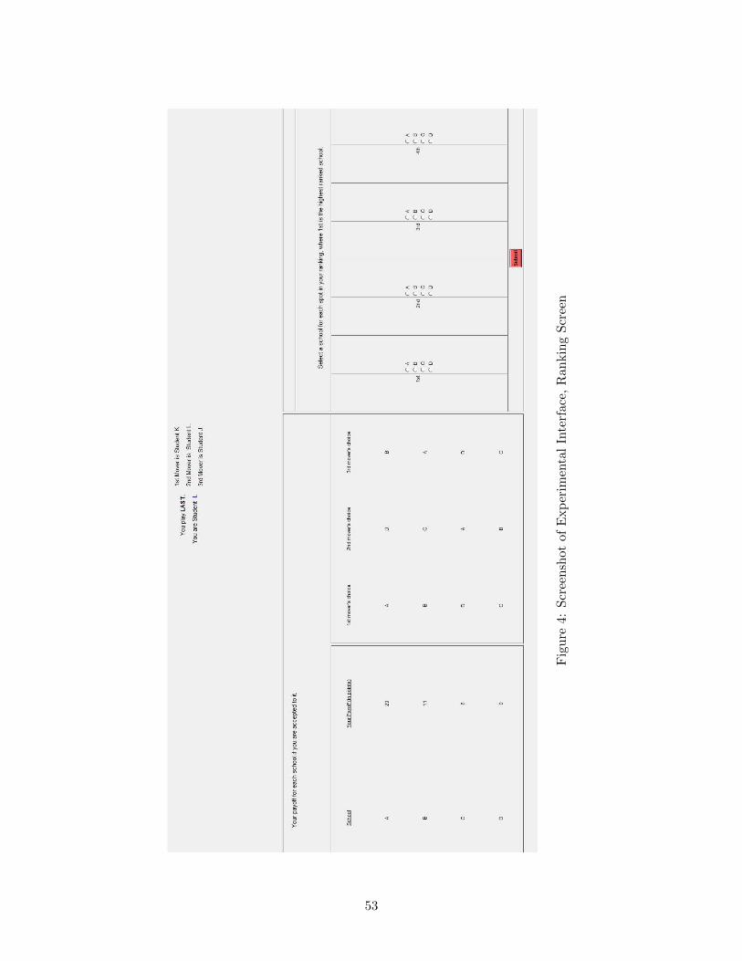
Fig

ure

4:S

cree

nsh

otof

Exp

erim

enta

lIn

terf

ace,

Ran

kin

gS

cree

n

53

Table 1: Pareto Efficiency by Mechanism and Game Type, Assigned Rank

(1) (2)Sim Seq

BM 1.870 1.805(0.042) (0.043)

DA 1.938 1.942(0.037) (0.038)

Difference -0.067 -0.138(0.056) (0.058)∗∗

N 800 800

Notes: This table measures Pareto efficiency by the assigned rank of students: lower average ranksare associated with higher efficiency. Assigned rank equals one when a student is assigned to hermost preferred school, two when assigned to her second most preferred school, three when assignedto her third most preferred school, and four when assigned to her least preferred school. For thisand subsequent tables, standard errors are in parentheses; ∗, ∗∗, and ∗ ∗ ∗ denote significance atthe 10%, 5%, and 1% level, respectively.

Table 2: Pareto Efficiency by Mechanism and Game Type, Earnings/Period

(1) (2)Sim Seq

BM 13.803 14.345(0.289) (0.300)

DA 13.283 13.342(0.264) (0.269)

Difference 0.520 1.003(0.392) (0.403)∗∗

N 800 800

Notes: This table measures Pareto efficiency by earnings per period. Earnings per period equals 20when a student is assigned to her most preferred school, U [10, 15] when assigned to her second mostpreferred school, U [4, 9] when assigned to her third most preferred school, and 0 when assigned toher least preferred school. We use the notation U [a, b] to refer to the discrete uniform distributionbetween a and b.

54

Table 3: Pareto Efficiency by Mechanism and Game Type, Separately by Role

Panel A: Simultaneous Games

(1) (2) (3) (4) (5)All Student i Student j Student k Student l

BM 1.870 1.800 1.890 2.610 1.180(0.042) (0.074) (0.078) (0.071) (0.039)

DA 1.938 1.750 1.740 2.880 1.380(0.037) (0.048) (0.046) (0.054) (0.049)

Difference -0.067 0.050 0.150 -0.270 -0.200(0.056) (0.088) (0.090)∗ (0.089)∗∗∗ (0.062)∗∗∗

N 800 200 200 200 200

Panel B: Sequential Games

(1) (2) (3) (4) (5)All Student i Student j Student k Student l

BM 1.805 1.560 1.680 2.740 1.240(0.043) (0.066) (0.080) (0.069) (0.043)

DA 1.942 1.720 1.730 2.900 1.420(0.038) (0.047) (0.051) (0.059) (0.050)

Difference -0.138 -0.160 -0.050 -0.160 -0.180(0.058)∗∗ (0.081)∗∗ (0.095) (0.091)∗ (0.066)∗∗∗

N 800 200 200 200 200

Notes: This table measures Pareto efficiency by the assigned rank of students: lower average ranksare associated with higher efficiency. Panel A considers only periods when students submittedpreferences simultaneously. Panel B considers only periods when students submitted preferencessequentially. See the notes to Table 1 for details.

55

Table 4: Pareto Efficiency in Game 1

Panel A: Simultaneous Games

(1) (2) (3) (4) (5)All Student i Student j Student k Student l

BM 2.025 2.100 2.075 2.800 1.125(0.065) (0.106) (0.097) (0.096) (0.053)

DA 1.975 1.900 1.900 3.050 1.050(0.060) (0.048) (0.048) (0.035) (0.035)

Difference 0.050 0.200 0.175 -0.250 0.075(0.089) (0.117)∗ (0.109) (0.102)∗∗ (0.063)

N 320 80 80 80 80

Panel B: Sequential Games

(1) (2) (3) (4) (5)All Student i Student j Student k Student l

BM 1.888 1.675 1.950 2.850 1.075(0.071) (0.097) (0.143) (0.092) (0.042)

DA 2.075 2.025 1.975 3.125 1.175(0.061) (0.025) (0.025) (0.082) (0.061)

Difference -0.188 -0.350 -0.025 -0.275 -0.100(0.094)∗∗ (0.100)∗∗∗ (0.145) (0.123)∗∗ (0.074)

N 320 80 80 80 80

Notes: This table measures Pareto efficiency by the assigned rank of students: lower average ranksare associated with higher efficiency. Panel A considers only periods when students submittedpreferences simultaneously. Panel B considers only periods when students submitted preferencessequentially. See the notes to Table 1 for details.

56

Table 5: Pareto Efficiency in Game 2

Panel A: Simultaneous Games

(1) (2) (3) (4) (5)All Student i Student j Student k Student l

BM 1.450 1.333 1.333 2.067 1.067(0.049) (0.088) (0.088) (0.046) (0.046)

DA 1.450 1.200 1.200 2.200 1.200(0.066) (0.092) (0.092) (0.092) (0.092)

Difference 0.000 0.133 0.133 -0.133 -0.133(0.080) (0.131) (0.131) (0.094) (0.094)

N 200 50 50 50 50

Panel B: Sequential Games

(1) (2) (3) (4) (5)All Student i Student j Student k Student l

BM 1.450 1.200 1.200 2.200 1.200(0.054) (0.074) (0.074) (0.074) (0.074)

DA 1.325 1.100 1.100 2.050 1.050(0.056) (0.069) (0.069) (0.050) (0.050)

Difference 0.125 0.100 0.100 0.150 0.150(0.080) (0.107) (0.107) (0.100) (0.100)

N 200 50 50 50 50

Notes: This table measures Pareto efficiency by the assigned rank of students: lower average ranksare associated with higher efficiency. Panel A considers only periods when students submittedpreferences simultaneously. Panel B considers only periods when students submitted preferencessequentially. See the notes to Table 1 for details.

57

Table 6: Pareto Efficiency in Game 3

Panel A: Simultaneous Games

(1) (2) (3) (4) (5)All Student i Student j Student k Student l

BM 2.083 1.867 2.200 2.900 1.367(0.087) (0.150) (0.169) (0.154) (0.089)

DA 2.144 1.875 1.850 3.050 1.800(0.055) (0.073) (0.067) (0.087) (0.064)

Difference -0.060 -0.008 0.350 -0.150 -0.433(0.099) (0.155) (0.165)∗∗ (0.167) (0.107)∗∗∗

N 280 70 70 70 70

Panel B: Sequential Games

(1) (2) (3) (4) (5)All Student i Student j Student k Student l

BM 2.050 1.767 1.800 3.133 1.500(0.086) (0.141) (0.139) (0.133) (0.093)

DA 2.119 1.725 1.800 3.100 1.850(0.057) (0.071) (0.089) (0.060) (0.057)

Difference -0.069 0.042 0.000 0.033 -0.350(0.099) (0.147) (0.158) (0.134) (0.104)∗∗∗

N 280 70 70 70 70

Notes: This table measures Pareto efficiency by the assigned rank of students: lower average ranksare associated with higher efficiency. Panel A considers only periods when students submittedpreferences simultaneously. Panel B considers only periods when students submitted preferencessequentially. See the notes to Table 1 for details.

58

Table 7: Tests of Equilibrium Play for Each Treatment

Panel A: Equilibrium Strategies

(1) (2)Sim Seq

BM 0.838(0.018)

DA 0.795 0.757(0.020) (0.021)

N 400 800

Panel B: Truth-Telling

(1) (2)Sim Seq

BM 0.605 0.545(0.024) (0.025)

DA 0.795 0.757(0.020) (0.021)

N 800 800

Panel C: Stability

(1) (2)Sim Seq

BM 0.640 0.530(0.048) (0.050)

DA 0.840 0.840(0.037) (0.037)

N 200 200

Notes: This table provides summary statistics that address equilibrium play, with different panelsrepresenting the appropriate test for different treatments. Panel A provides the rates of play in linewith equilibrium, which is the appropriate test of equilibrium play for sequential BM, sequentialDA, and simultaneous DA. Specifically, for sequential BM, Panel A provides the rates of play inaccordance with the sequential BM equilibrium conjecture; because truth-telling is an equilibriumstrategy for DA, Panel A provides the rates of truth-telling for sequential DA and simultaneous DA.Next, Panel B provides the rates of truth-telling. Finally, Panel C provides the rates of stability(i.e., the proportion of matchings that are stable), which is the appropriate test of equilibrium playfor simultaneous BM. The unit of observation in Panels A and B is a student-period, while the unitof observation in Panel C is a group-period.

59

Table 8: Pareto Efficiency by Order of Moves when Equilibrium is Played, Sequential Games Only

Panel A: Student k Later

(1) (2) (3) (4) (5)All Student i Student j Student k Student l

BM 1.662 1.471 1.471 2.471 1.235(0.083) (0.125) (0.125) (0.125) (0.106)

DA 1.554 1.357 1.357 2.357 1.143(0.088) (0.133) (0.133) (0.133) (0.097)

Difference 0.108 0.113 0.113 0.113 0.092(0.121) (0.183) (0.183) (0.183) (0.146)

N 124 31 31 31 31

Panel B: Student k Earlier

(1) (2) (3) (4) (5)All Student i Student j Student k Student l

BM 1.614 1.303 1.303 2.697 1.152(0.067) (0.081) (0.081) (0.081) (0.063)

DA 1.964 1.857 1.857 2.857 1.286(0.075) (0.078) (0.078) (0.078) (0.101)

Difference -0.351 -0.554 -0.554 -0.160 -0.134(0.103)∗∗∗ (0.120)∗∗∗ (0.120)∗∗∗ (0.120) (0.113)

N 216 54 54 54 54

Notes: This table measures Pareto efficiency by the assigned rank of students: lower average ranksare associated with higher efficiency. Only periods when students submitted preferences sequentiallyare considered because no order of moves exists for simultaneous move games. Only periods whereall four students played an equilibrium strategy are considered. Equilibrium strategies are thesequential BM equilibrium conjecture for sequential BM and truth-telling up to the district schoolfor DA. Panel A considers only periods when Student k moved later than either Student i or Studentj. Panel B considers only periods when Student k moved earlier than both Students i and j. Seethe notes to Table 1 for details.

60