a theory of sequential fragmentation and its astronomical

J. Astrophys. Astr. (1989) 10, 89–112 A Theory of Sequential Fragmentation and Its Astronomical Applications Wilbur K. Brown Lassen College, Susanville, California 96130, USA Received 1987 May 21; revised 1988 November 15; accepted 1988 December 1

Abstract. A theory of sequential fragmentation is presented that describes a cascade of fragmentation and refragmentation, i.e., continued comminution. It is shown that the theory reproduces one of the two major empirical descriptors that have traditionally been used to describe the mass distributions from fragmentation experiments. Additional experimental evidence is presented to further validate the theory, and includes explosive aerosolization, grinding in a ball mill, and simulated volcanic action. Also presented are some astronomical applications of the theory including infalling extraterrestrial material, siderophile concentrations in black magnetic spherules of possible meteoritic origin, the asteroids, the distribution of galactic masses, and the initial mass function of stars.

Key words: sequential fragmentation—infalling extraterrestrial material—meteoritic spherules—asteroids—galactic masses—initial mass function

1. Introduction

The problem of analytically characterizing the distribution of particles from fragmentation experiments has almost always been approached empirically. Ideally, it should be possible to derive the desired analytical description from a physical theory of fragmentation. In this article, I present my theory of “sequential fragmentation,” or fragmentation that occurs progressively—as in continued comminution: following a fragmentation event, the resulting fragments are caused to refragment, and so on down the chain. I assume that there is no continuing feed replenishment.

There are several empirical descriptions of fragment distributions. Typically, whendata were limited, the simplest description has been used—that of a power law. Forexample,

N (> m) = Cm – b. (1)

Here m is the fragment mass, N ( > m) is the cumulative number of fragments of massgreater than m, and b and C are constants. Historically, a great deal of work hasconcerned the size distribution, rather than the mass distribution. Difficulties were experienced in characterizing the size of particles (e.g., broken coal) which was not easy to describe owing to the typically irregular shapes of the fragments. In this article, I will reduce all data to that of the pertinent mass distribution—which I consider to be the basic quantity involved.

90 W. K. Brown

When more extensive data are acquired, it is usually found that power laws like Equation (1) are inadequate, and more sophisticated empirical descriptions are required. Turcotte (1986) has reviewed these relations, and I will address each of them in turn below.

An extensively used empirical description is

(2)

where NT is the total number of fragments, µ is a mass related to the average mass of the distribution, and v is a free parameter. Equation (2) has enjoyed considerable success, but I emphasize that its use has been entirely empirical.

Another successful empirical description has been the Weibull distribution: (3)

Here M( < l) is the cumulative mass of fragments of size less than l, MT is the total mass of fragments in the distribution, σ is a size related to the average size, and k is a free parameter.

A third successful empirical description of fragment size distribution is that of Rosin & Rammler (1934; see also Kittleman 1964). In the language of this article, theRosin–Rammler law of crushing is given by

(4) Because

(5) it can be seen that the Rosin–Rammler distribution is identical to the Weibull distribution.

Finally, the lognormal distribution has been extensively used (e.g., Loveland & Trivelli 1927). In essence, it is

(6)

where n(l) is the differential size distribution, and A and a are constants. In contrast to the above analytical descriptions, the lognormal distribution does have a mathemat- ical basis (McAlister 1879), although even it has no derivation based on physical theory. Therefore, Equations (1)–(6) have been used entirely empirically: their useserved only to summarize and correlate data, and their extrapolation beyond therange of the data was risky. In addition, as a result of their empirical use, these analytical descriptions could not yield any physical understanding of the fragmentation phenomena involved.

In the following sections, I first present my sequential fragmentation theory. I then test the theory by applying it to the description of the fragment distributions from several terrestrial sequential fragmentation phenomena. Further, I apply the theory to the description of what may be the results of sequential fragmentation phenomena in the field of astronomy: infalling extraterrestrial material, siderophile element concen-trations in black magnetic spherules of possible cosmic origin, the asteroids, the

Sequential Fragmentation on Astronomical Scales 91 distribution of galactic luminosities, and the stellar initial mass function. Finally, with all these results in hand, I discuss the meaning of the principal free parameter of the sequential fragmentation theory.

2. The sequential fragmentation theory I start my theory of sequential fragmentation with the equation

(7) Here, n(m) is the particle number distribution with dimensions of the number of fragments per unit mass of mass between m and m + dm. The function f (m’ → m) describes the mass distribution that results when a single heavy fragment of mass m’(>m) breaks up into lighter pieces. The symbol c denotes a constant. Equation (7) is a summing of the contribution to the particle number distribution at m, by all masses m’ greater than m.

I choose for the function f (m’→ m)

(8) where the fragment mass in the right-hand-side argument is m, not m´. In Equation (8),γ is a free parameter (– 1 γ < 0), and m 1 is a mass related to the average fragment mass in the distribution n(m). I chose Equation (8) (Brown 1986c) because I felt that inthe fragmentation of a particle of mass m´, the resulting single-event mass distribution,f , must contain a disproportionately large number of lighter particles. That is, lighter particles would be formed preferentially. I also chose the power-law form expressed by Equation (8) both because it was the simplest one I could think of, and because I intuitively felt it was correct. I will now support my choice of Equation (8) withexperimental data.

Gaudin (1926) found that the “fines” produced in his mills were a prominent featureof his mass distributions, but distinct from that of the coarser particles. Finding that the fines yielded a straight line on a log–log plot of “the percentage of material” vs thescreen aperture, Gaudin characterized the fines distribution by the equivalent of

(9) where Δ M/MT is the mass fraction selected between a series of screens differing in size by a fixed ratio. Thus the mass distribution in Equation (9) is given in terms of mass per logarithmic interval in size (or mass) and as I shall show later, this quantity is given by m2n(m). Therefore, the mass distribution, f (m´ → m), is functionally relatedto Equation (9) by

(10)

where we may identify γ with (k/3) – 1. The mass distribution of Equation (10) is of atype that falls in the category of Equation (1). Gaudin suggested that the fines had

92 W. K. Brown been “protected” by the larger fragments in his mills, and would therefore be the result of single-event fragmentations. Gaudin found that in his roll mill, Galena gave values of k all across the range 0.84 < k < 0.92 (– 0.72 < γ < – 0.69), while Quartz gave 0.80 < k < 0.91 (– 0.73 < γ < – 0.70). Further, he found that in his rod mill, Quartz gave the result 0.55 < k < 0.94 (– 0.81 < γ < – 0.69). Gaudin’s calculations allowed for 0.4 < k <1.2 (– 0.87 < γ < – 0.6). These results strongly support the use of Equation (8).

More recently, research has been carried out to find the single-event mass distribu-tion directly (Gilvarry 1961; Gilvarry & Bergstrom 1961; Bergstrom 1962). Bergstrom characterized his fines data with the equivalent of

(11)

which is just an approximation (for l/σ≪ 1) to the Weibull distribution of Equa- tion (3). Gilvarry & Bergstrom refer to Equation (11) as the “empirical Schuhmann Law,” and to k as the “Schuhmann size modulus,” but I have not been able to obtain a copy of their reference (Schuhmann 1940). I will show later that for particles of low mass, Equation (11) yields

(12) just as in Equation (10). Bergstrom (1962) found that in fracturing glass spheres by squeezing them between a parallel pair of extremely hard tungsten carbide platens, he obtained the value k= 1.16, so that γ = – 0.61. There was found to be no effect when the strain rate was varied. Gaudin’s and Bergstrom’s results show that the power-law form of Equation (8) is on firm experimental ground.

When Equation (8) is inserted into Equation (7) and c is chosen as m1– l , I obtain

(13)

The solution to this, for – 1 < γ < 0, is

(14)

where the expression has been normalized so that

(15) For the special case γ = — 1,

(16)

where Κ is a constant (the total number of fragments, N T is undefined in this case).The mass distribution for a sequential fragmentation for — 1 < γ < 0 is given by and

(17)

Sequential Fragmentation on Astronomical Scales 93 and for γ = – 1 by

(18) i.e., a constant

In Fig. 1, are examples of plots of the mass distribution of Equation (17). When such shapes were seen as that on the left-hand-side of Fig. 1, they were called “skew” toexpress the fact that they did not look like the normal curve of error. The plot on theright-hand-side in Fig. 1 illustrates that the sequential fragmentation mass distribution has lognormal-like qualities (Equation 6).

Fig. 2 comprises log–log plots of the mass distribution mn(m). (In this article I will use “log” to denote the logarithm to the base 10.) As we shall see, it is usually necessary to use log–log plots to describe data, and it is convenient to make decades the same length on the ordinate and on the abscissa. This type of plot provides a consistent means by which one can easily recognize the shapes depicted in Fig. 2.

The quantity mn(m) describes the mass distribution in terms of the total mass of fragments of mass m between m and m + dm. However, mn(m) also symbolizes the number of particles per logarithmic interval in m, and because the theory and data must usually be plotted υs log m, it is useful to think of mn(m) in this way. We shall

Figure 1. Examples of mass distributions yielded by the sequential fragmentation theory. The linear plot at left shows the “skew” character of the distribution. At right, it can be seen that the distribution has lognormal-like qualities, especially on the right-hand side of the curve where the data always seem to fall.

Figure 2. Examples of sequential fragmentation mass distributions plotted in the “standard”way adopted for this article. The curves have been shifted vertically and horizontally, but theshapes are correct.

94 W. K. Brown later see that the mass distribution, mn(m), bears a simple relationship to the size distribution. Because mn(m) may be interpreted as the number of particles per natural logarithmic interval in m, the quantity m2n(m) symbolizes the mass distribution interms of the total mass of fragments per logarithmic interval in m(dM/d ln m = m2 n(m)). This fact was used earlier in the formulation of Equation (10). The m2n(m) form is quite similar to a lognormal distribution.

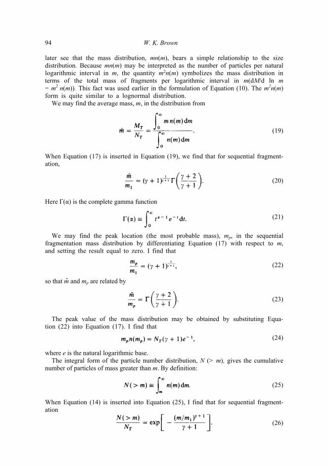
We may find the average mass, m, in the distribution from (19)

When Equation (17) is inserted in Equation (19), we find that for sequential fragment-ation, (20)

Here Γ(α) is the complete gamma function

(21)

We may find the peak location (the most probable mass), mp, in the sequential fragmentation mass distribution by differentiating Equation (17) with respect to m, and setting the result equal to zero. I find that (22)

so that m and mp are related by (23)

The peak value of the mass distribution may be obtained by substituting Equa-

tion (22) into Equation (17). I find that (24)

where e is the natural logarithmic base. The integral form of the particle number distribution, N (> m), gives the cumulative

number of particles of mass greater than m. By definition: (25)

When Equation (14) is inserted into Equation (25), I find that for sequential fragmentation

(26)

-

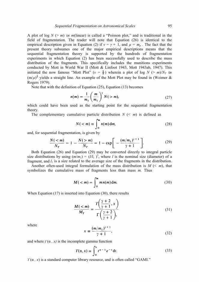
Sequential Fragmentation on Astronomical Scales 95 A plot of log N (> m) υs m(linear) is called a “Poisson plot,” and is traditional in thefield of fragmentation. The reader will note that Equation (26) is identical to theempirical description given in Equation (2) if ν = γ + 1, and µ = mp . The fact that the present theory subsumes one of the major empirical descriptions means that the sequential fragmentation theory is supported by the hundreds of fragmentation experiments in which Equation (2) has been successfully used to describe the mass distribution of the fragments. This specifically includes the munitions experiments conducted by Mott in World War II (Mott & Linfoot 1943, Mott 1943ab, 1947). This initiated the now famous “Mott Plot” (v = ½ ) wherein a plot of log N (> m)/NT υs (m/µ) ½ yields a straight line. An example of the Mott Plot may be found in (Weimer & Rogers 1979).

Note that with the definition of Equation (25), Equation (13) becomes

(27) which could have been used as the starting point for the sequential fragmentationtheory.

The complementary cumulative particle distribution N (< m) is defined as

(28) and, for sequential fragmentation, is given by

(29)

Both Equation (26) and Equation (29) may be converted directly to integral particle size distributions by using (m/m1) = (l/l1 )3, where l is the nominal size (diameter) of afragment, and l1 is a size related to the average size of the fragments in the distribution.

Another often-used integral formulation of the mass distribution is M (< m), thatsymbolizes the cumulative mass of fragments less than mass m. Thus When Equation (17) is inserted into Equation (30), there results (31)

(32) and where (α , x) is the incomplete gamma function

(33) Υ (α , x) is a standard computer library resource, and is often called “GAMI.”

(30)

where

Υ

Υ

96 W. K. Brown

Finally, we may write down the expression for M (> m), i.e., the cumulative mass ofall fragments of mass greater than m

(34) I note that

(35) where Γ(α, x) is the complementary incomplete gamma function (“GAMIC”): (36)

Then, using Equations (17), (32), (34), (35) and (36), I find that

(37) Again, the integral distributions M (< m) and M (>m) may be converted directly tosize distributions by setting (m/m1) = (l/l1)3.

I feel that the integral functions M and Ν are more difficult to assess visually, andthat therefore, mn(m) is preferable. I admit that using log mn(m) υs log m plots also distorts the shape of the distribution (see Figs 1 and 2), but this form is necessary to describe data over the wide range in mass usually available. In the following studies of various types of fragmentation data, I will reduce whatever form the data are in to log mn(m) vs log m.

3. Terrestrial tests of the theory

3.1 High Explosive Aerosolization In an explosive fragmentation experiment named “Operation Roller Coaster” (Shreve & Thomas 1965), a pyrophoric metal was aerosolized. The detonation of the explosive drove the expansion and provided the initial mechanical motion of the material.The aerosolization process occurred through a combination of boiling (phase trans- formations under high temperature and pressure), mechanical fragmentation, aero-dynamic breakup, and combustion. This is surely an example of sequential fragmentation.

Fig. 3 shows the data yielded by three samples collected from the Operation Roller Coaster explosion in the form of log l υs M (< l) plotted on probability paper. Toreduce this to mn(m), I note from the definitions of M (< m) and M (> m) inEquations (30) and (34)

(38)

Sequential Fragmentation on Astronomical Scales 97

Figure 3. The integral mass distribution data yielded by the Operation Roller Coaster plutonium aerosolization experiment. The aerosol size distribution is plotted on probability paper.

If the density, ρ , is constant from fragment to fragment, then the mass and nominal size, l, of fragments are related by (39)

(40)

and if dm from Equation (40) is inserted in Equation (38), there results

(41) To extract dM /dl from Fig. 3, I plotted Μ vs l, and obtained the derivative graphically as a function of l Alternatively, one may define the log–log slope, S1, as

(42)

The slope, S1, may be obtained by plotting log Μ υs log l and determining S1

graphically. Then, from Equations (41) and (42)

(43)

Then

98 W. K. Brown Fig. 4 shows the Operation Roller Coaster data plotted as log mn(m) vs l3 ( ∝ mass).The data curves in Fig. 4 are almost coincident over the central range, but diverge atthe extremes. The best fit of the data with the present theory was obtained using γ = – 0· 95 in Equation (17) plotted with NT = 1. As I will discuss later, a value of γ so near to – 1 means that the process consisted of relatively few sequential fragmentation events.

With regard to Equation (41), it can be seen that dM/dl is a crucial quantity. This quantity is obtainable directly from shifting samples of particles through screens of progressively smaller mesh size. ∆l is the mesh size difference between two adjacent screens, and ∆Μ is the mass of particles caught on the lower of the two screens. Data are often found in the form ∆M /MT (%) in a size range ∆l.

The data from the aerosolization type of experiment are often described by the empirical Weibull distribution, Equation (3), with k 1. It is therefore useful tocompare the Weibull distribution directly with the sequential fragmentation mass distribution Analytically, I find that for the Weubul distribution

(44)

where (m/m2) = (l/σ)3. Using Equation (38), I find that

(45) This was used earlier in the formulation of Equation (12) for the fines in thedistribution.

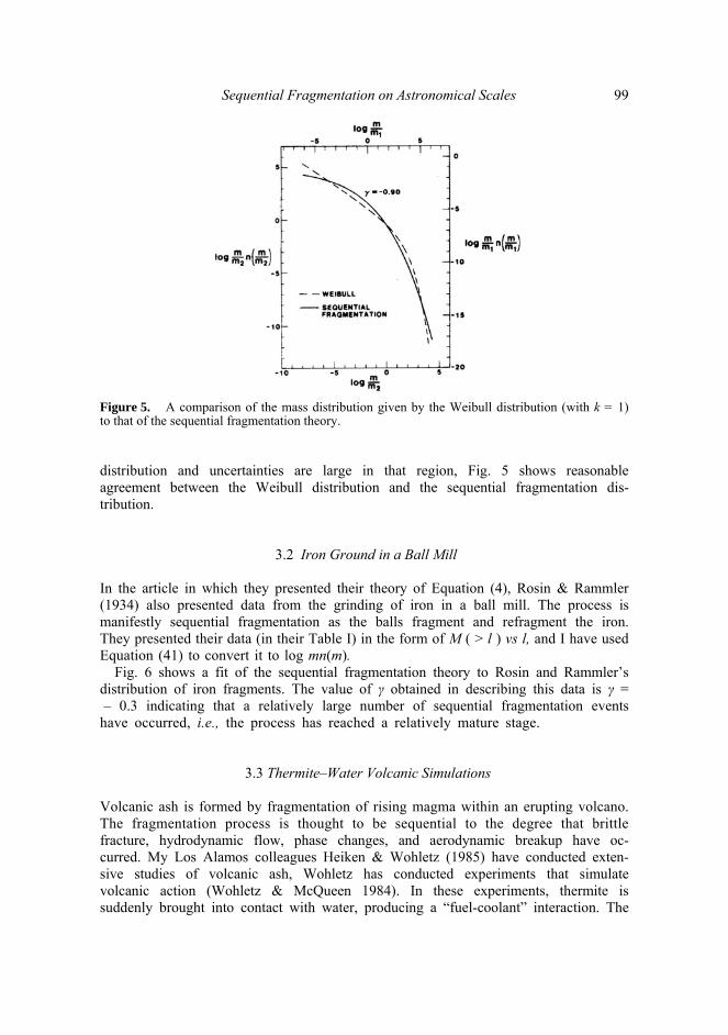
Fig. 5 shows a comparison of the Weibull distribution with that of sequential fragmentation made over the same range in mass as that of the Roller Coaster experiment. Note that Equation (45) contrasts fundamentally with Equation (17), because it differs by one power of m in the fines end of the distribution. Consideringthe fact that the fines are usually only fairly well characterized by the Weibull

Figure 4. The mass distribution yielded by the Operation Roller Coaster aerosolizationexperiment compared to the sequential fragmentation theory.

≃


Figure 5. A comparison of the mass distribution given by the Weibull distribution (with k = 1) to that of the sequential fragmentation theory. distribution and uncertainties are large in that region, Fig. 5 shows reasonable agreement between the Weibull distribution and the sequential fragmentation distribution.

3.2 Iron Ground in a Ball Mill In the article in which they presented their theory of Equation (4), Rosin & Rammler (1934) also presented data from the grinding of iron in a ball mill. The process is manifestly sequential fragmentation as the balls fragment and refragment the iron. They presented their data (in their Table I) in the form of M ( > l ) vs l, and I have usedEquation (41) to convert it to log mn(m).

Fig. 6 shows a fit of the sequential fragmentation theory to Rosin and Rammler’s distribution of iron fragments. The value of γ obtained in describing this data is γ = – 0.3 indicating that a relatively large number of sequential fragmentation events have occurred, i.e., the process has reached a relatively mature stage.

3.3 Thermite–Water Volcanic Simulations Volcanic ash is formed by fragmentation of rising magma within an erupting volcano.The fragmentation process is thought to be sequential to the degree that brittlefracture, hydrodynamic flow, phase changes, and aerodynamic breakup have oc-curred. My Los Alamos colleagues Heiken & Wohletz (1985) have conducted extensive studies of volcanic ash, Wohletz has conducted experiments that simulate volcanic action (Wohletz & McQueen 1984). In these experiments, thermite is suddenly brought into contact with water, producing a “fuel-coolant” interaction. The

100 W. Κ. Brown

Figure 6. The mass distribution of iron particles, ground in a ball mill, compared to thesequential fragmentation theory. resulting ash is collected and sieved, to give data in the form of ∆M/MT (%) υs l. Equation (41) was used to translate these data into the log mn(m) vs log m form.

Fig. 7 shows the mass distribution of the ash from a thermite-water volcanicsimulation. The best-fit value of γ = – 0.94 indicates that there was time for relativelyfew sequential fragmentation generations to take place before the action terminated.

In addition, Wohletz kindly provided me with particle size data on a sample of volcanic ash taken at La Mesita, a site just below Los Alamos on the Rio Grande. The La Mesita ash is thought to have been formed in part by a fuel-coolant interaction inwhich rising magma contacts groundwater or lake water resulting in explosive vapour production and hydrodynamic instabilities. Fig. 8 shows the mass distribution of particles in the La Mesita volcanic ash sample. A value of γ = – 0.96 was obtained for this case.

Because the value of γ for the La Mesita ash is less than that for the simulated ash, a simple conclusion is that the natural fragmentation process did not advance as far as that produced experimentally in the thermite-water simulations.

Continuing studies of volcanic ash distributions (Wohletz et al. 1989) support the wide application of sequential fragmentation theory to many volcanic processes such as saltation, etc.

3.4 Experimental Support In this section, I have presented comparisons of the sequential fragmentation theory to data from several terrestrial experiments that clearly represent instances of continued comminution. Taken together with the hundreds of experiments in which the data sets were described by Equation (2) (that has been shown to be reproduced by the present theory), I believe that the totality of supporting experimental evidence validates the sequential fragmentation theory. I would claim that the simple logic of the sequential fragmentation theory, as exemplified by Equation (7) or (27), and Equation (8), even gives the theory a degree of beauty.

Be that as it may, in the next section I analyze various astronomical data that Ispeculate have been produced by the sequential fragmentation process, but in. which


Figure 7. The mass distribution of ash particles, yielded by a thermite-water volcanicsimulation, compared to the sequential fragmentation theory.

Figure 8. The mass distribution of volcanic ash particles, from a sample taken at the LaMesita site near Los Alamos, compared to the sequential fragmentation theory. the actual processes are difficult or impossible to observe. As usual in the field of astronomy, we normally must be content to remain on earth and observe the phenomena as they appear at present.

4. Astronomical applications of the theory

4.1 Infalling Extraterrestrial Material Material falling from outside into the atmosphere must fragment and refragment as it breaks up from aerodynamic forces and the heat of air friction. It is a likely candidate for having undergone the sequential fragmentation process.

Parkin & Tilles (1968) have summarized the data observed for the infalling rate of extraterrestrial material. Sea sediments, polar ice, air, and space were searched for the amount and character of interplanetary debris.

102 W. K. Brown

Fig. 9 shows Parkin and Tilles’ plot of log N ( > m) (per unit time) vs log m. From the definition of N ( > m) and N (< m) in Equations (25) and (28), we see that

(46)

For completeness, I note that this can be changed into the dN /dl form by substitutingEquation (40) into Equation (46). I also note that dN /dl = n(l). See Section 4.2 below.

Thus, in general, from such a plot as Fig. 9, we must find dN /dm. However, most of the data shown in Fig. 9 are in the form of straight lines. Such a straight line may be described by

(47)

Here, N (0) is the ordinate where the line (or its extension) crosses the abscissa log m = 0, and S2 is the log–log slope:

(48)

Combining the last three equations, I find that

(49)

that also yields line segments on a log mn(m) υs log m plot. Thus, to obtain the mass distribution in this case, one must obtain N (0) and S2 from Fig. 9. Fig.10 shows Parkin and Tilles’ data as transformed by Equation (49).

The best fit of the present theory to the observed infall of extraterrestrial material is given by using γ = – 0.98 in Equation (17). It can be seen from Fig. 10 that although the “IRONS” don’t fit well, the remainder of the materials do. A value of γ so near to — 1 means that there was time for relatively few sequential fragmentation events totake place before the process ceased.

Figure 9. Parkin and Tilles’ (1968) graph summarizing the integral particle distributions of infalling extraterrestrial material. The cumulative number influx to Earth (number of particles per square metre per day with mass greater than m (grams)).


Figure 10. The mass distribution of infalling extraterrestrial material compared to thesequential fragmentation theory.

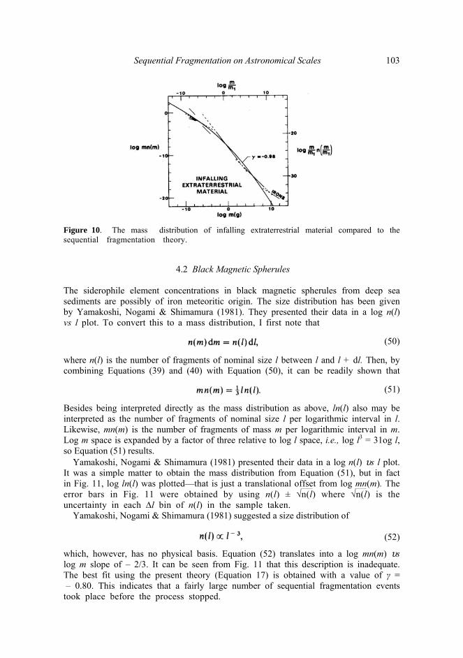
4.2 Black Magnetic Spherules The siderophile element concentrations in black magnetic spherules from deep sea sediments are possibly of iron meteoritic origin. The size distribution has been given by Yamakoshi, Nogami & Shimamura (1981). They presented their data in a log n(l) vs l plot. To convert this to a mass distribution, I first note that

(50)

where n(l) is the number of fragments of nominal size l between l and l + dl. Then, by combining Equations (39) and (40) with Equation (50), it can be readily shown that

(51)

Besides being interpreted directly as the mass distribution as above, ln(l) also may be interpreted as the number of fragments of nominal size l per logarithmic interval in l. Likewise, mn(m) is the number of fragments of mass m per logarithmic interval in m. Log m space is expanded by a factor of three relative to log l space, i.e., log l3 = 31og l, so Equation (51) results.

Yamakoshi, Nogami & Shimamura (1981) presented their data in a log n(l) υs l plot. It was a simple matter to obtain the mass distribution from Equation (51), but in fact in Fig. 11, log ln(l) was plotted—that is just a translational offset from log mn(m). Theerror bars in Fig. 11 were obtained by using n(l) ± √n(l) where √n(l) is theuncertainty in each ∆l bin of n(l) in the sample taken.

Yamakoshi, Nogami & Shimamura (1981) suggested a size distribution of

(52)

which, however, has no physical basis. Equation (52) translates into a log mn(m) υslog m slope of – 2/3. It can be seen from Fig. 11 that this description is inadequate. The best fit using the present theory (Equation 17) is obtained with a value of γ = – 0.80. This indicates that a fairly large number of sequential fragmentation events took place before the process stopped.

104 W. K.Brown

Figure 11 The mass distribution siderophile element concentrations in black magnetic spherules, obtained from deep-sea sediments, compared to the sequential fragmentation theory.

Although Yamakoshi, Nogami & Shimamura (1981) state that the spherules are not confirmed as to extraterrestrial origin (Doyle, Hopkins & Betzer 1976), they do present evidence that the majority of the spherules are of iron meteoritic origin. It is a pity that the extraterrestrial “IRONS” of the preceding section do not fit with γ = – 0.98, because the spherules, with γ = – 0.80, have clearly undergone more exten-sive processing in the sequential fragmentation cascade.

The size distribution n(l), that gives the number of particles per unit length of length l between l and l + dl, in sequential fragmentation may be obtained with the use of Equation (51). It is given by

(53) Equation (53) is a Weibull distribution (as is Equation 14). M. Felthauser (1988) hascarried out a comparative study of this distribution and the lognormal distributionwith regard to certain observed particle size distributions.

4.3 The Asteroids Repetitive collisions between the asteroids may have resulted in their present mass distribution. If so, it seems reasonable to see if the sequential fragmentation theory fits the observed data.

The size distribution of the asteroids is relatively well known. The pertinent articles are (Kuiper et al. 1958; Anders 1965; Hartmann & Hartmann 1968; Hartmann 1969; Davis et al. 1985). Donnison & Sugden (1984) studied the size distribution of the asteroids, but they used a theoretical distribution with no physical basis.

I used the data given by Davis et al. (1985) in the form of log n(l) vs log l. As before, I used Equation (51) to achieve my Standard log mn(m) υs log m plot.

The mass distribution of the asteroids is shown in Fig. 12. The famous “bump,” lying in the range 6 < log l3 < 7 is obvious. However, the difference between thepresent theory (with γ = – 0.95) and the observed mass distribution in the bump is


Figure 12 The mass distribution of the asteroids compared to the sequential fragmentationtheory. only ∆log ln(l) ~ 0.25 or a multiplicative factor of ~ 1.8. The fact that γ is again – 1 indicates that relatively few sequential fragmentation events have occurred, butwhence came the bump?

The present theory describes two opposing simultaneous processes on this scale: fragmentation and gravitational accretion (assumed proportional to the mass of each fragment). However, soon after the solar system was formed, before the present stage was reached, there must have been a period of pure accretion. In the spirit of Equation (7), I model this pure acretion process by

(54) where now m > m, and every collision results in a new particle of composite mass m(k1 is a positive constant). Differentiating Equation’(54) yields

(55) I assume for the moment that n(0) is a constant, so that

(56) where k2 is another positive constant. If I let k2 = m– l, I find that

(57) where m3 is a mass related to the average mass. Then the particle number distribution is

(58) where the constant k3 is positive. From Equation (58) we see that n(0) is indeed a constant, as assumed above.

The mass distribution for pure accretion is given by

(59)

≃

´

3

106 W. K.Brown At large masses, m is limited by the amount of material originally present so the mass distribution would fall off at large m. Equation (59) could indicate the progenitor of the “bump” that has not yet been erased by the later, but immature ( γ = – 0.95) sequential fragmentation process. I might point out that early accretion of theplanetary material might also have followed Equation (59).

4.4 Galactic Masses Ostriker & Cowie (1981) and Ikeuchi (1981) have proposed a mechanism of galaxy formation in which a pre-galactic star explodes as a supernova, and a massive shell is ejected. As the shell moves outward, sweeping up mass, the shell cools and fragments into clouds that form stars more massive than the original star. The process is presumed to continue until bodies of galactic mass are achieved. Thus the authors have named this mechanism “explosive amplification.” The literature may be followed backward from (Bertschinger 1985).

If indeed it was the explosive amplification mechanism that generated galaxies, then the present theory of sequential fragmentation ought to describe the observed massdistribution of galaxies. I assume here that the amplification was proportional, i.e., when a fragment sweeps up additional mass, the fragment gains mass in proportion toits original mass. If this is so, then the shape of the fragment mass distribution wouldnot change, and Equation (17) would still apply.

Unfortunately, the mass distribution of galaxies is not well known, but rather it isthe distribution of total galactic luminosities that is reasonably well known. The dataare often represented by the empirical Schecter (1976) distribution

(60) where n* and L* are constants, L /L* is the variable and α is an adjustable parameter. If I assume that the mass/luminosity ratio (M/L) is constant, then I can compare thesequential fragmentation mass distribution with the Schecter distribution.

For the purposes of direct comparison, I write

(61) and note that this is identical to Equation (17) for the case α = γ = 0. Such a value of αis possible, but not probable. A value of γ = 0 would indicate an extremely protractedprocess of sequential fragmentation.

A modification of the Schecter distribution, proposed by Dressier (1978) involves the use of the form exp ( – Lp) in Equations (60) and (61). This would result in (62)

In this form the luminosity distribution can be made to agree identically with Equation (17) of sequential fragmentation, with the identification of γ with α and of pwith γ + 1. If this were done, then α, the log–log slope of the faint end of the galacticluminosity distribution, would take on a new meaning as the single-event massdistribution, as in Equation (8). However, one more variable, p, has been introduced.


If I limit my attention to the case p = 1, then I must do the best I can in fitting Equation (61) with the sequential fragmentation mass distribution. Fig. 13 shows the comparison for α = – 1.0 (Turner & Gott 1976) and the best fit of γ = – 0.4. I note that the bright end of the distribution is well-approximated by the sequential fragmentation theory even though p = 1 in the pure exponential cutoff as compared with the more complex cutoff function of Equation (17). I also note that a wide range of α has been found from observations (– 1.6 ≲ α ≲ 0) depending on the sample of

galaxies studied (see, e.g., Sandage, Tammann & Yahil 1979; Tammann, Yahil & Sandage 1979), so that I am not too concerned about the poor agreement at the faint end in Fig. 13. However, in this regard, I must call attention to the superior ability of the Weibull distribution to approximate the Schecter distribution (Brown 1986a) throughout the entire range.

The value γ = – 0.4 provides a reasonable fit to the distribution of galactic luminosities. This indicates that if explosive amplification/sequential fragmentation as actually responsible for defining the galaxies as we see them today, then a relatively large number of sequential fragmentation events must have occurred before the “top-down” process stopped. When sufficient data are available, it will be possibleto apply the sequential fragmentation theory to the mass distribution of intergalacticLyman α clouds (Ikeuchi & Ostriker 1986).

In another study of how galaxies might have formed (Brown 1985) I explored the idea that galaxies might have resulted from eddies in a turbulent early universe. In Brown (1986b) I postulated a mass distribution of eddies based on a sequentialfragmentation process of eddy-spawning. This now needs to be modified to bring it into agreement with Equation (17).

4.5 The Stellar Initial Mass Function When the concept of “explosive amplification” is applied to stars, the star formation scenario is that after galaxies were formed, explosive amplification continued viaSupernovae. As a star undergoes a supernova event, a shell is ejected that cools, sweeps

Figure 13. The distribution of total galactic luminosities (as given by the Schecter distribution)compared to the sequential fragmentation theory.

108 W. Κ. Brown up additional mass, and separates into fragments as the shell moves outward. When any particular fragment has gathered enough mass, it will, in turn, undergo a supernova explosion and perpetuate the cascade of sequential fragmentation. I have hypothesized (Brown 1986c) that this mechanism results in (1) the initial mass function (IMF) as deduced from stellar absolute luminosities, e.g., (Miller & Scalo 1979), and (2) solar systems (Brown & Gritzo 1986, Brown 1987a, b,c). However, the analysis of (Brown 1986c) must be modified due to an error I made that has resulted in a change in the low-mass end of the sequential fragmentation distribution. The results do not have to be modified much because the strong cutoff function at the high-mass end remains unchanged. In my opinion, explosive amplification is closely related to self- propagating star formation (see the recent article by Schulman & Seiden 1986 and references therein).

Fig. 14 shows a fit of the present theory (Equation (17)) to the IMF, ξ (Μ), of Miller & Scalo (1979). In the present analysis, the best fit was obtained with γ = – 0.80, and this indicates that the supernova shell fragmentation process is fairly mature. Of course, it has had ample time to get that way since shortly after the Big Bang about (15 ± 3) × 109 years ago. However, it is really the number of sequential fragmentation events that matters, and not just the time available to the process.

I consider the fit in Fig. 14, of the IMF with the present theory, to be excellent, although it can be seen that the sequential fragmentation theory overestimates theIMF at low masses. I believe that this is due to the fact that below ~ 8 M , Type II Supernovae cannot occur. Thus, stars of < 8 Μ do not contribute to the distribution at lower masses, and the observed mass distribution falls below the sequential fragmentation theory at these lower masses. It is a pity that the predictive power of Equation (17) begins to fail below 1 Μ , because it would have been helpful to extrapolate the IMF down into the region of brown dwarves and “Jupiters.” This would have allowed an assessment of how much “dark matter” might be available from this source. However, assuming explosive amplification is a credible mechanism

Figure 14. The stellar initial mass function ξ (M), of Miller and Scalo 1979 compared to thesequential fragmentation theory. For stellar masses above M = 1 (solar mass units),the twocurves are coincident.

Sequential Fragmentation on Astronomical Scales 109 for self-propagating star formation, I do not hesitate to extrapolate the sequential fragmentation theory of the IMF to higher masses.

5. Discussion I will now discuss the possible meaning of the key parameter γ, as defined in Equation (8) and as it is manifested in Equations (14) and (17). It seems clear that γ = γ(t) where t is the time after the beginning of the process. More accurately, γ(t) symbolizes how far the sequential fragmentation process has progressed, i.e., how mature the process is. To illustrate this, we may envision that shortly after the sequential fragmentation process begins, we will have one fragment of unit mass, two of mass one-half, four of mass one-quarter, etc. Thus at the beginning, the particle number distribution, n(m), will have a log–log slope of – 1, and γ (0) = – 1, as in Equation (16). This idealistic picture assumes no depletion due to sequential fragmentation. However, in the absence of feed replenishment, the particle number distribution will be progressively depleted, especially at large fragment mass. It is this progressive depletion that curves the mass distribution and changes the value of γ. The mass distribution, mn(m), is peaked at mid-range mass (Fig. 2). This is due to the fact that although there are many more particles of low mass, there is not much mass in the distribution at low particle mass.

As can be seen from Fig. 2, as the sequential fragmentation process matures, the mass distribution grows increasingly more peaked at midrange mass as γ(t) increases (becomes less negative). I prefer to think of this progression as being related to γ(t) + 1, as in Equation (17), i.e., the greater the number of events that have occurred, the larger γ(t) + 1 is. Because I suppose that γ + 1 can grow progressively larger, I do not rule out values of γ 0 in the present theory.

Table 1 summarizes the results of the applications presented in earlier sections of this article.

The maturity of the sequential fragmentation process depends on the number of generations of fragmentation events that have taken place. If the rate of occurrence of generations in the cascade is denoted by R (t), then the number of generations, , at Table 1. Results of various applications of the sequential fragmentation theory.

110 W. K.Brown the time t is given by

(63)

The relationship between (t) and γ(t) + 1 is unknown, but it must rise mono-tonically from γ (0) + 1 = 0. It is clear that both the refragmentation rate and the time duration of the fragmentation events dictate the maturity of the sequential fragmen- ation process.

It appears that the quantity γ (t) + 1 can be used as a discriminator between samples of fragments. If two samples are characterized by different values of γ (t) + l, then they must have been processed in different ways.

As can be seen from the plots of Equation (17) in Fig. 2, the width of the mass distribution is inversely related to γ + 1. I have been able to show that the right-handside of the distributions (the only part of the distributions I have found useful in this article), the half-width at half maximum (HWHM) In (m 1/2 /m1), is given by

(64)

When I compare this to the actual HWHM I find that

(65)

to within about 0.02% in the range (– 1 < γ < 0). If, as in the lognormal distribution, I define for the sequential fragmentation distribution (66)

then (67)

Values of σ for the applications studied in this article are included in Table 1. As (γ + 1) increases, σ decreases, signifying that the mass distribution is progressively depleted at higher masses as the sequential fragmentation process matures.

So, three meanings of γ have been identified: (1) the log–log slope of a single-event fragmentation event (Equation 8), (2) an indicator of the maturity of the sequential fragmentation process, and (3) the standard deviation of the sequential fragmentation mass distribution. In addition, because it seems possible to describe a class of fragmentation mass distributions with a single variable, γ, the sequential fragmentation process may be an example of fractal structure. Indeed, this application offractals has been advanced by Turcotte (1986) for many observed fragmentation mass distributions.

6. Conclusions The present theory of sequential fragmentation appears to describe many phenomenaonon widely differing scales. Of the applications studied for this article, all were

Sequential Fragmentation on Astronomical Scales 111 successfully fit with mass distributions yielded by the theory. In addition, the theory subsumes one of the two major empirical descriptors of data. I am satisfied that the theory is validated.

I would like to emphasize three things: (1) the theory has only one adjustable parameter, γ; (2) the fit of each data set is unique in that when the tilt and curvature are matched, the value of γ is closely bounded; and (3) the parameter γ appears to have meaning as the log–log slope of the mass distribution resulting from a single-event fragmentation, as an indicator of the maturity of the sequential fragmentation process and as the standard deviation of the sequential fragmentation mass distribution Another point worth stressing is that the sequential fragmentation mass distribution is based on a physical theory, i.e., a theory derived from a physical model.

Applications of the present theory (other than those studied here) suggest them- selves. Orbiting space junk is clearly undergoing sequential fragmentation and because its presence is a hazard to astronauts and satellites, characterizing its mass distribution is important. The particles in the rings around the giant planets should follow the present theory. During the formation of our solar system, the mass distribution of the planetesimals—as might be inferred from the crater distributionson Mercury, the Moon, and Mars—could be described by sequential fragmentationtheory. Another possibility is the mass distribution of the chondrules in meteorites.

I am most pleased that my sequential fragmentation theory describes a certain class of ordinary events, and I look forward to future applications of the theory.

Acknowledgements I am grateful to my three referees (especially S. Ikeuchi, University of Tokyo) who pointed out a fundamental error in the initial version of this article. To propagate the error beyond (Brown 1986c) would have been unfortunate.

References Anders, Ε. 1965, Icarus, 4, 399. Bergstrom, Β. Η. 1962, in Proc. 5th U.S. Symp. Rock Mech., p. 155. Bertschinger, E. 1985, Astrophys. J., 295, 1. Brown, W. K. 1985, Astrophys. Space Sci., 115, 257. Brown, W. K. 1986a, Astrophys. Space Sci., 121, 351. Brown, W. K. 1986b, Astrophys. Space Sci., 126, 255. Brown, W. K. 1986c, Astrophys. Space Sci., 122, 287. Brown, W. K. 1987a, Earth, Moon and Planets, 37, 225. Brown, W. K. 1987b, Publ. astr. Soc. Pacific, 99, 858. Brown, W. K. 1987c, Los Alamos National Laboratory report LA-11005. Brown, W. K., Gritzo, L. A. 1986, Astrophys. Space Sci., 123, 161. Davis, D. R., Chapman, C. R., Weidenschilling, S. J., Greenberg, R. 1985, Icarus, 62, 30. Donnison, J. R., Sugden, R. A. 1984, Μon. Not. R. Astr. Soc., 210, 673. Doyle, L. J., Hopkins, Τ. L., Betzer, P. R. 1976, Science, 94, 1157. Dressler, Α. 1978, Astrophys. J., 223, 765. Felthauser, Μ. Α. 1988, MS Thesis, Colorado State Univ., Fort Collins. Gaudin, A. M. 1926, Trans. AIME, 73, 253. Gilvarry, J. J. 1961, J. Appl. Phys., 32, 391. Gilvarry, J. J., Bergstrom, Β. Η. 1961, J. Appl. Phys., 32,400. Hartmann, W. K. 1969, Icarus, 10, 201.

112 W. K. Brown Hartmann, W. Κ., Hartmann, A. C. 1968 Icarus, 8, 361. Heiken, G., Wohletz, K. H. 1985, Volcanic Ash, Univ. of California Press.Ikeuchi, S. 1981, Publ. astr. Soc. Japan, 33, 211. Ikeuchi, S., Ostriker, J. 1986, Astrophys. J., 301, 522. Kittleman, L. R. jr. 1964, J. Sedimentary Petrology, 34, 483. Kuiper, G. P., Fujita, Y., Gehreis, T., Groeneveld, I., Kent, J., Van Biesbroeck, G.,

Van Houten, J. 1958, Astrophys. J. Suppl., 3, 289. Loveland, R. P., Trivelli, A. P. H. 1927, J. Franklin, Inst., 204, 377. McAlister, D. 1879, Proc. R. Soc. London, 29, 367.Miller, G. E., Scalo, J. M. 1979, Astrophys. J. Suppl., 41, 513. Mott, N. F. 1943a, Ministry of Supply report AC-3642, Great Britain. Mott, N. F. 1943b, Ministry of Supply report AC-4035, Great Britain. Mott, N. F. 1947, Proc. R. Soc. London Ser. Α., 189, 300. Mott, N. F., Linfoot, E. F. 1943, Ministry of Supply report AC-3348, Great Britain. Ostriker, J. P., Cowie, L. L. 1981, Astrophys. J., 243, L127. Parkin, D. W., Tilles, D. 1968, Science, 159, 936. Rosin, P., Rammler, Ε. 1934, Kolloid-Zeitschrift, 67, 16. Sandage, Α., Tammann, G. Α., Yahil, A. 1979, Astrophys. J., 232, 352. Schecter, P. 1976, Astrophys. J., 203, 297. Schuhmann, R. 1940, Am. Inst. Mining, Met., Petrol. Engrs. Tech. Publ. No. 1189. Schulmann, L. S., Seiden, P. E. 1986, Science, 233, 425.Shreve, J. D. jr., Thomas, D. M. C. 1965, U.S. Dept. of Defence report DASA-1644. Tammann, G. Α., Yahil, Α., Sandage, Α. 1979, Astrophys. J., 234, 775. Turcotte, D. L. 1986, J. Geophys. Res., 91, 1921. Turner, Ε. L., Gott, J. R. III. 1976, Astrophys. J., 209, 6 Weimer, R. J., Rogers, H. C. 1979, J. Appl. Phys., 50, 8025. Wohletz, K. H., McQueen, R. G. 1984, Geology, 12, 591. Wohletz, Κ. Η., Sheridan, Μ. F., Brown, W.K. 1989, J. Geophys. Res., Submitted.Yamakoshi, Κ., Nogami, Κ., Shimamura, Τ. 1981, J. Geophys. Res., 86, 3129.

a theory of sequential fragmentation and its astronomical

Documents