sequential monitoring of the tail behavior of … monitoring of the tail behavior of dependent data...
TRANSCRIPT
Sequential monitoring of the tail behavior of dependent data
Yannick Hoga∗, Dominik Wied†
August 16, 2016
Abstract
We construct a sequential monitoring procedure for changes in the tail index and extreme quan-tiles of β-mixing random variables, which can be based on a large class of tail index estimators.The assumptions on the data are general enough to be satisfied in a wide range of applications.In a simulation study empirical sizes and power of the proposed tests are studied for linear andnon-linear time series. Finally, we use our results to monitor Bank of America stock log-losses from2007 to 2012 and detect changes in extreme quantiles without an accompanying detection of a tailindex break.
Keywords: Sequential monitoring, change point, β-mixing, tail index, extreme quantiles, func-tional central limit theoremJEL classification: C12 (Hypothesis Testing), C14 (Semiparametric and Nonparametric Meth-ods), C22 (Time-Series Models)
1 Motivation
The tail index of a random variable is arguably one of the most important parameters of its distribution:
It determines some fundamental properties like the existence of moments, tail asymptotics of the
distribution and the asymptotic behavior of sums and maxima. As a measure of tail thickness, the
tail index is used in fields where heavy tails are frequently encountered, such as (re)insurance, finance,
and teletraffic engineering (cf. Resnick, 2007, Sec. 1.3, and the references cited therein). Particularly
in finance, the closely related extreme quantiles play a prominent role as a risk measure called Value-
at-Risk (VaR).
The use of the variance as a risk measure has a long tradition in finance. Under Gaussianity the
variance completely determines the tails of the distribution, which is no longer the case with heavy-
tailed data. Hence, in order to assess the tail behavior of a time series, practitioners often estimate
the tail index or an extreme quantile, the implicit assumption being their constancy over time. There
are several suggestions in the literature on how to test this crucial assumption: Quintos, Fan and
∗Faculty of Economics and Business Administration, University of Duisburg-Essen, Universitatsstraße 12, D-45117Essen, Germany, tel. +49 201 1834365, [email protected]. The author gratefully acknowledges the supportof DFG (HA 6766/2-1).†University of Cologne and TU Dortmund, Germany, tel. +49 221 4704514, [email protected]. Fi-
nancial support by Deutsche Forschungsgemeinschaft (SFB 823) is gratefully acknowledged.The authors would like to thank Stefan Fremdt for helpful discussion and Christoph Hanck for carefully reading anearlier version of this manuscript.
1
Phillips (2001) developed so called recursive, rolling and sequential tests for independent and GARCH
data for tail index constancy based on the Hill (1975) estimator. Kim and Lee (2011) investigated
their tests for more general β-mixing time series. Taking a likelihood approach for independent data,
Dierckx and Teugels (2010) focus on breaks in the tail index for environmental data. Tests based on
other estimators than the Hill (1975) estimator were first proposed by Einmahl, de Haan and Zhou
(2016) for independent and Hoga (2016+) for dependent data. To the best of our knowledge the only
paper dealing with changes in extreme quantiles is Hoga (2015). All these tests are of a retrospective
nature.
We are not aware of any work on online surveillance methods for constancy of the tail index
and extreme quantiles. This is important because, as noted in Chu, Stinchcombe and White (1996),
‘[b]reaks can occur at any point, and given the costs of failing to detect them, it is desirable to detect
them as rapidly as possible. One-shot tests cannot be applied in the usual way each time new data
arrive, because repeated application of such tests yields a procedure that rejects a true null hypothesis
of no change with probability one as the number of applications grows.’ This paper will fill this gap
for closed-end procedures. To allow for sufficient flexibility in the use of tail index estimators, we will
use the approach of Hoga (2016+).
Whether a monitoring procedure for a change in the tail index or an extreme quantile is of interest
will largely be a matter of context. If interest centers on VaR, which is widely used in the banking
industry and by financial regulators as a risk measure, the quantile monitoring procedure will be more
relevant. If however interest centers on the mean excess function of the (log-transformed) data X,
then, since E (logX − log t|X > t) converges to the extreme value index of X as t→∞, the tail index
alternative seems more appropriate. Furthermore, the tail index per se could also be of interest as
there are indications that it has predictive power for stock returns (Kelly and Jiang, 2014), where
higher (lower) tail indices of returns indicate higher (lower) absolute returns.
The outline of this paper is as follows. The main results under the null and two alternatives
are stated in Section 2, where an example of a time series satisfying our assumptions is also given.
Simulations and an empirical application are presented in Sections 3 and 4 respectively. All proofs
are collected in an appendix.
2 Main results
2.1 Preliminaries and assumptions
To introduce the required notation let X1, . . . , Xn be a sequence of random variables defined on some
probability space (Ω,A, P ) with survivor function Fi (x) := 1− Fi(x) = P (Xi > x), that is regularly
varying with parameter −αi (written Fi ∈ RV−αi), i.e.,
Fi (x) = x−αiLi (x) , x > 0, (1)
2

where Li : (0,∞)→ (0,∞) is slowly varying, i.e.,
limx→∞
Li (λx)
Li (x)= 1 ∀ λ > 0. (2)
If Xi is Pareto distributed, then Li(x) ≡ c > 0. Since slow variation of the function Li(x) means,
loosely speaking, that it behaves like a constant function at infinity, we say that Xi with tails as in (1)
has Pareto-type tails. In the context of extreme value theory, αi is called the tail index and γi := 1/αi
the extreme value index (Resnick, 2007, Sec. 4.5.1).
Define
Ui (x) := F−1i
(1− 1
x
), x > 1,
as the(1− 1/x
)-quantile, F−1i being the left-continuous inverse of Fi. Then, recall that (1) is equiv-
alent to
Ui(λx)
Ui(x)−→
(x→∞)λγ (3)
(e.g., Resnick, 2007, Prop. 2.6 (v)). Throughout, k = kn ∈ N will denote a sequence satisfying
k ≤ n− 1,
k −→(n→∞)
∞ andk
n−→
(n→∞)0, (4)
controlling the number of upper order statistics used in the estimation of the tail index and p = pn → 0,
n → ∞, will denote a sequence of small probabilities, for which we want to test for a change in an
appertaining extreme (right-tail) quantile Ui(1/p). As is customary in extreme value theory, we will
usually drop the subindex n and simply write k and p. For t− s ≥ 1/n and y ∈ [0, 1] set
Xk (s, t, y) :=(⌊k (t− s) y
⌋+ 1)
-th largest value of Xbnsc+1, . . . , Xbntc.
Under the assumption of strictly stationary Xi we write F = Fi and U = Ui. Let
γ(s, t) := γn (s, t) , 0 ≤ s < t <∞, t− s ≥ 1/n,
denote a generic tail index estimator based on the(⌊k(t− s)
⌋+ 1
)-largest order statistics of the
subsample Xbnsc+1, . . . , Xbntc. Then approximate with (3) for x = 1/p, λ = pn/k with small p > 0 to
get
U
(1
p
)≈ U
(n
k
)(pn
k
)−γ≈ Xk(s, t, 1)
(np
k
)−γ(s,t)=: xp(s, t), (5)
which motivates and defines the so called Weissman (1978) estimator for the extreme quantile U(1/p).
Hence, the idea is to use the (within sample range) estimator Xk(s, t, 1) of U(n/k) to estimate the
(possibly out of sample range) quantile U(1/p) by exploiting the regular variation of the quantile
function in (3). In view of this we will require p k/n.
3

For concreteness we will focus in the following on the Hill (1975) estimator of γ given by
γH(0, 1) :=1
k
k−1∑i=0
log
(Xn−i:nXn−k:n
), (6)
where Xn:n ≥ Xn−1:n ≥ . . . ≥ X1:n denote the order statistics of the sample X1, . . . , Xn. But the
main results in Theorems 1 and 2 below hold without modification for the moments-ratio estimator
of Danıelsson et al. (1996) and the class of estimators introduced by Csorgo and Viharos (1998); see
also the proof of Theorem 1 below.
The dependence concept we will use in the following is that of β-mixing, that is for a sequence of
random variables Xii∈N the β-mixing coefficients β (l) converge to zero:
β (l) := supm∈N
E
supA∈F∞m+l+1
∣∣P (A|Fm1 )− P (A)∣∣ −→
(l→∞)0,
where F∞m := σ (Xm, Xm+1, . . .) and Fml := σ (Xl, . . . , Xm). For more on this mixing concept we refer
to Bradley (1986).
Write D[a, b] for the space of cadlag functions on [a, b] (0 ≤ a < b <∞) endowed with the Skorohod
topology and D(I), I ⊂ R2 compact, for the two-parameter extension.
In order to construct a monitoring procedure for a tail index change, we have to assume tail index
(or, equivalently, extreme value index) constancy over some historical period (also called training
period) of suitable length n:
(A1) γ1 = . . . = γn, n ∈ N.
This assumption can of course be tested by any of the retrospective change point tests proposed in,
e.g., Hoga (2016+, 2015).
As soon as a period X1, . . . , Xn of tail index or extreme quantile stability is identified and more
observations Xn+1, Xn+2, . . . become available, we are interested in an online surveillance method
testing
H0,γ : γ1 = . . . = γn = γn+1 = . . . vs.
H≶1,γ : γ1 = . . . = γn = . . . = γbnt∗c ≶ γbnt∗c+1 = γbnt∗c+2 = . . . ,
(7)
and
H0,U : U1
(1
p
)= . . . = Un
(1
p
)= Un+1
(1
p
)= . . . vs.
H≶1,U : U1
(1
p
)= . . . = Un
(1
p
)= . . . = Ubnt∗c
(1
p
)≶ Ubnt∗c+1
(1
p
)= Ubnt∗c+2
(1
p
)= . . .
(8)
for some t∗ ≥ 1 denoting the unknown change point. We use H0 or H≶1 as shorthand notation for
both of H0,γ , H0,U or H≶1,γ , H≶
1,U .
4

We use the following detectors for (7)
V γn (t) :=
[(t− 1)
(γ (1, t)− γ (0, 1)
)]2´ 1t0
[s(γ (0, s)− γ (0, 1)
)]2ds, t ≥ 1 + t0,
W γn (t) :=
[t0(γ (t− t0, t)− γ (0, 1)
)]2´ 1t0
[t0(γ (s− t0, s)− γ (0, 1)
)]2ds, t ≥ 1 + t0,
and for (8)
Vxpn (t) :=
[(t− 1) log
(xp(1,t)xp(0,1)
)]2´ 1t0
[s log
(xp(0,s)xp(0,1)
)]2ds
, t ≥ 1 + t0,
Wxpn (t) :=
[t0 log
(xp(t−t0,t)xp(0,1)
)]2´ 1t0
[t0 log
(xp(s−t0,s)xp(0,1)
)]2ds
, t ≥ 1 + t0,
where t0 > 0 defines the (minimal) fraction of n upon which the tail index and extreme quantile
estimators are based. To motivate our detectors consider V γn , the others can be motivated similarly.
In the numerator the training period estimate γ(0, 1) is compared with the current observation period
estimate γ(1, t). If the observation period length (t − 1) is large, that difference is weighted more
heavily. The denominator ‘self-normalizes’ the numerator. While we could have chosen a wide range
of functionals for this (e.g., the denominator of W γn ), it seemed more natural to incorporate the
functional form of the numerator to do so. With this motivation in mind we are inclined to reject H0
if the following stopping times terminate (in the sense of being finite):
τVγ
n := inft ∈ [1 + t0, T ] : V γ
n (t) > c,
τWγ
n := inft ∈ [1 + t0, T ] : W γ
n (t) > c,
and
τVxp
n := inft ∈ [1 + t0, T ] : V
xpn (t) > c
,
τWxp
n := inft ∈ [1 + t0, T ] : W
xpn (t) > c
,
where from now on inf ∅ :=∞ and c > 0 is chosen, such that under H0, limn→∞ P (τn <∞) = α for
some prespecified significance level α ∈ (0, 1) (see Theorem 1 below). Here T > 1 denotes the arbitrar-
ily large closed end of the procedure, i.e., the method terminates after observations Xn+1, . . . , XbnT c.
Closed-end procedures are quite common, e.g., Aue et al. (2012) consider breaks in portfolio betas,
Wied and Galeano (2013) breaks in cross-correlations, Zeileis et al. (2005) and Aschersleben et al.
(2015) breaks in regression and cointegrating relationships respectively.
5

Remark 1. (a) The detector V γn comes closer in spirit to many of the detectors in the online moni-
toring literature, where an estimate of some parameter based on the historical period is compared
to that based on the (ever longer) monitoring period; see the references in the paragraph before.
However, the procedure based on V γn is not consistent against H>1,γ , cf. Theorem 2 below, which
is the reason for introducing the method based on W γn .
(b) We could have based our procedure equally well on detectors of the type
V γn (t) :=
1
σ2γ,γ
[(t− 1)
√k(γ (1, t)− γ (0, 1)
)]2,
where σ2γ,γ is a consistent estimator of the asymptotic variance of√k(γ(0, 1)− γ) based on the
observations X1, . . . , Xn in the observation period (e.g., the one in Theorem 2 of Hoga (2016+)).
It turned out however, that in simulations values of even n = 500 for the training period were
not sufficient to deliver accurate variance estimates for a wide range of model parameters for the
models we investigated, which lead to severe size distortions of our surveillance methods. This
is why we opted for the self-normalized approach advocated in Shao and Zhang (2010) in our
sequential setting. To the best of our knowledge we are the first to do so. Shao and Zhang (2010)
found that for retrospective change point tests self-normalized test statistics delivers far superior
size in simulations. However, the price to be paid for using a self-normalization approach vs. a
variance estimation approach is slightly lower power.
Under H0 we will assume beyond (A1) that:
(A2) Xii∈N is a strictly stationary β-mixing process with continuous marginals and mixing coeffi-
cients β (·), such that
limn→∞
n
rnβ (ln) +
rn√k
log2(k) = 0 (9)
for sequences lnn∈N ⊂ N, rnn∈N ⊂ N tending to infinity with ln = o(rn), rn = o(n).
(A3) There exists a function r = r (x, y), such that for all x, y ∈ [0, y0 + ε] (y0 ≥ 1, ε > 0)
limn→∞
n
rnk
∑1≤i,j≤rn
Cov
IXi>U( n
kx), I
Xj>U(nky
) = r (x, y) .
(A4) For some constant C > 0
n
rnkE
rn∑i=1
IU(nky
)<Xi≤U( n
kx)4
≤ C(y − x) ∀ 0 ≤ x < y ≤ y0 + ε, n ∈ N.
(A5) There exist ρ < 0 and a function A(·) with eventually positive or negative sign, limt→∞A(t) = 0,
such that for any y > 0
limt→∞
U(ty)U(t) − y
γ
A(t)= yγ
yρ − 1
ρ,
where√kA(n/k)→ 0 as n→∞.
6

For the detectors for changes in extreme quantiles we need the following further assumptions:
(A6) limn→∞npk = 0, limn→∞ k
−1/2 log (np) = 0.
(A7) The sequence k satisfies
U(1/p)
U(n/k
) (npk
)γ− 1 = o
(1√k
).
The conditions (A2)-(A4) correspond (almost) exactly to conditions (C1), (C2) and (C3*) in
Drees (2000). Condition (A5), which is a widely used second-order strengthening of (3) (e.g., Kim
and Lee, 2011; Einmahl et al., 2016), is stronger than Drees’s (2000) condition (3.5). (A2) ensures
a standard ‘big block - small block’ approach may be applied to deduce weak convergence of what
Einmahl et al. (2016, p. 42) termed the simple sequential tail empirical process in (A.1) below. The
limit process has a well-defined covariance structure by virtue of (A3). (A6) provides a range
for p: limn→∞npk = 0 provides an upper bound for the decay of p (indicating the limitations of the
extreme value theory approach towards the center of the distribution) while limn→∞ k−1/2 log
(np/k
)=
limn→∞ k−1/2 log (np) = 0 provides a lower bound, beyond which estimation is no longer feasible. Note
that if the d.f. obeys the quite general expansion
1− F (x) = Cx−α(1 +O(x−β)) as x→∞; C,α, β > 0,
then by inversion U(x) = C1/αx1/α(1 + O(x−β/α)), whence (A7) does not impose an additional
constraint on the choice of k.
2.2 Results under the null and the alternative
We are now ready to state the main results under the null, describing the asymptotic behavior of our
monitoring procedures based on the stopping rules τn.
Theorem 1. Suppose (A1)-(A5) hold for y0 = 1. Then for any t0 > 0, T > 1 + t0 and
Vt0,T :=supt∈[1+t0,T ]
[W (t)− tW (1)
]2´ 1t0
[W (s)− sW (1)
]2ds
,
Wt0,T :=supt∈[1+t0,T ]
[W (t)−W (t− t0)− t0W (1)
]2´ 1t0
[W (s)−W (s− t0)− t0W (1)
]2ds
,
(10)
withW (t)
t∈[0,T ] a standard Brownian motion,
(i) under H0,γ
limn→∞
P(τV
γ
n <∞)
= P(Vt0,T > c
),
limn→∞
P(τW
γ
n <∞)
= P(Wt0,T > c
),
7
(ii) under H0,U and additionally (A6)-(A7)
limn→∞
P(τV
xp
n <∞)
= P(Vt0,T > c
),
limn→∞
P(τW
xp
n <∞)
= P(Wt0,T > c
).
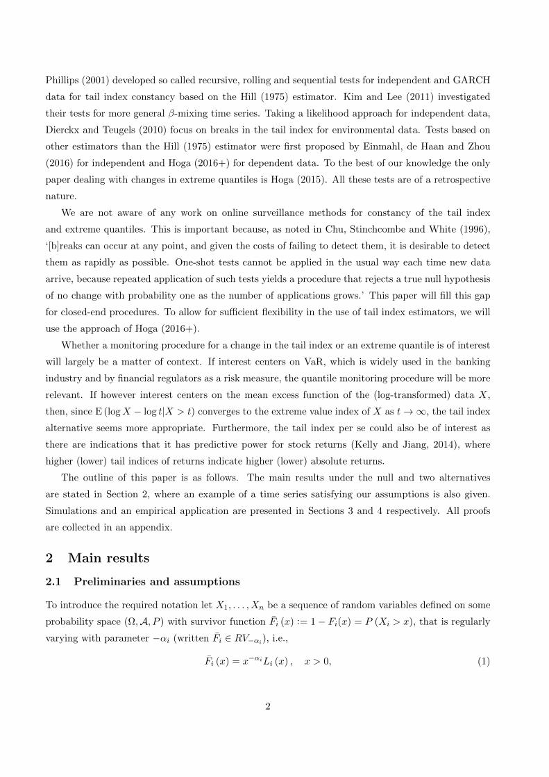
Next, we investigate the behavior of our procedures under the ‘one-sided’ alternativesH≶1 . To prove
our results the observations will be denoted by the triangular array of random variables Xn,i, n ∈ N,
i = 1, . . . , n, which have a common marginal survivor function F pre ∈ RV−αpre (F post ∈ RV−αpost) for
i ∈ Ipre :=
1, . . . , bnt∗c
(i ∈ Ipost :=bnt∗c+ 1, . . . , bnT c
). Set
Upre(x) = F−1pre
(1− 1
x
)and Upost(x) = F−1post
(1− 1
x
).
Theorem 2. Let the triangular array of observationsXn,i
n∈N,i=1,...,n
be given by
Xn,i :=
Yn, i ∈ Ipre,Zn, i ∈ Ipost,
where Ynn∈N and Znn∈N both satisfy conditions (A2)-(A5) with y0 = T and
k, γpre, Upre(·), rpre(·, ·) and k, γpost, Upost(·), rpost(·, ·)
respectively. Then
(i)
limn→∞
P(τV
γ
n <∞)
= 1 under H<1,γ ,
limn→∞
P(τV
γ
n <∞)< 1 under H>1,γ ,
(ii)
limn→∞
P(τW
γ
n <∞)
= 1 under H≶1,γ ,
where under H>1 additionally t∗ ∈ [1, T − t0] must hold.
Suppose that additionally (A6)-(A7) hold for Yn and Zn. Then
(iii)
limn→∞
P(τV
xp
n <∞)
= 1 under H≶1,γ ,
(iv) if t∗ ∈ [1, T − t0] and |√k/ log(k/(np)) log(Upre(1/p)/Upost(1/p))| −→
(n→∞)∞,
limn→∞
P(τW
xp
n <∞)
= 1 under H≶1,U .
8

Remark 2. (a) Note that the sequence k in the pre- and post-break period must be the same. This
is however not too restrictive as (see (11) below) one can frequently choose k = nν for some
arbitrarily small ν > 0. So if (A2)-(A7) are satisfied for k = nν with ν ∈ (0, νpre) for the pre-
break period and with ν ∈ (0, νpost) in the post-break period, then taking ν ∈ (0,min(νpre, νpost))
leads to a sequence for which all assumptions are satisfied for the whole sample.
(b) If the Xn,i are generated as in Theorem 2, the hypothesis H≶1,γ is a strict subset of the hypothesis
H≶1,U . E.g., taking Zn = aYn, a 6= 1, is covered under H≶
1,U , but not under H≶1,γ , since scaling
does not affect the tail index. If however (e.g.) H>1,γ is true, we have Upre/Upost ∈ RVγpre−γpost>0
and hence
Upre(1/pn)
Upost(1/pn)−→
(n→∞)∞,
s.t. H>1,U is true.
(c) Under H>1 the procedure based on τVγ
n is not consistent, which motivated the study of τWγ
n .
The reason for the inconsistency is, simply speaking, that in a sample with one extreme value
index break, extreme value index estimators will consistently estimate the larger extreme value
index. Hence, if there is a break in t∗ toward lighter tails in the observation period, then γ(1, t),
t > t∗, will still estimate the larger extreme value index, even though the last part of the sample
upon which it is based possess a smaller extreme value index. Thus, the change goes unnoticed.
2.3 An Example
In this subsection we verify the conditions (A1)-(A4) for the following stochastic volatility model
Xi = σiZi, i ∈ Z,
where Zi are i.i.d. and independent from σi. Denote by 1 − F|Z| ∈ RV−α, α > 0, the survivor
function of |Z0|. The volatility process is assumed to be generated according to
σi = exp(Yi), where Yi =
∞∑j=0
ψjεi−j ,
with (w.l.o.g.) ψ0 = 1, εii.i.d.∼ N (0, σ2) and geometrically decreasing coefficients |ψj | =
(j→∞)O(ηj),
η ∈ (0, 1), covering all finite order ARMA(p,q)-models. Many popular stochastic volatility models use
(zero-mean) Gaussian AR(1)-models for the volatility dynamics (Asai et al., 2006).
We now verify our conditions for |Xi| = σi|Zi|. For (A2) strict stationarity is immediate (which
also implies (A1)). By Bradley (1986, Ex. 6.1) the Yi are geometrically β-mixing, whence, by Gaus-
sianity of the Yi, they are also geometrically ρ-mixing (Bradley, 1986, Eq. (1.7) & Thm. 5.1 and the
comments below it), i.e., the ρ-mixing coefficients
ρ(j) = supU∈L2(B0−∞)
V ∈L2(B∞j )
∣∣corr(U, V )∣∣ −→(j→∞)
0
9

decay to zero geometrically fast. Here, B0−∞ = σ(. . . , Y−1, Y0), B∞j = σ(Yj , Yj+1, . . .) and L2(A) is
the space of square-integrable, A-measurable real-valued functions. By Bradley (1986, p. 170) this
implies geometric ρ-mixing of σi = exp(Yi). This in turn implies geometric ρ-mixing of Xi = σiZi
since (by independence of the Zi) the ρ-mixing coefficients of Xi are bounded by those of σi, such
that geometric ρ-mixing is inherited from the volatility process (see Bradley, 2007, Thm. 6.6). We
conclude that ρ(j) ≤ Kηj for some η ∈ (0, 1) for the mixing coefficients ρ(·) appertaining to the |Xi|.By Bradley (2007, Thm. 6.6) again, independence of the Zi and recalling that the Yi (and hence the
σi) are geometrically β-mixing, the same holds true for the β-mixing coefficients of the |Xi|. Thus,
(A2) is satisfied for the following choices
k = nν for ν ∈ (0, 3/4), ln = −2log n
log η, rn = nν/3. (11)
We check conditions (C2) and (C3) of Drees (2003, Prop. 2.1), which implies (A3) because with
the above choices rnk/n = o(1). For (C2) we get from Hill (2011, Thm. 2.1) that as n→∞
P (|X1| > xU(n/k), |X1+m| > yU(n/k)) ∼E[σα1 σ
α1+m]
E[σα1 ] E[σα1+m]P (|X1| > xU(n/k))P (|X1+m| > yU(n/k))
∼E[σα1 σ
α1+m]
E[σα1 ] E[σα1+m]
k
nx−α
k
ny−α,
where the last line follows from (12) below and (e.g.) Resnick (2007, Sec. 2.2.1). (C3) is satisfied
due to geometric ρ-mixing of |Xi| (see also Drees, 2003, Rem. 2.2). Assumption (A4) is again a
consequence of Drees (2003, Prop. 2.1 & Rem. 2.3).
The |Xi| inherit their heavy tails from the Zi as, by Breiman’s (1965) lemma,
1− F (x) = P (|X0| > x) ∼(x→∞)
E[σα1 ]P (|Z0| > x). (12)
Hence, the |Xi| also have tail index α and (1) is satisfied. Of course, (12) only gives 1 − F (x) =
cx−α(1 + o(1)). This is weaker than
limt→∞
1−F (ty)1−F (t) − y
−α
A(1/[1− F (t)])= y−α
yρα − 1
ρ/α, (13)
with√kA(n/k) → 0 as n → ∞, which is equivalent to (A5) (cf. de Haan and Ferreira, 2006,
Thm. 2.3.9). The currently sharpest result on the second-order behavior of the d.f.s of stochastic
volatility models seems to be Kulik and Soulier (2011, Prop. 2.8). Assume
1− F|Z|(x) = czx−α exp
(ˆ x
1
η(s)
sds
), x > 0, c > 0
for some η(s) = O(sαρ), ρ < 0. For instance Frechet-, |tν |- and generalized Pareto distributions have
such tails (cf. Beirlant et al., 2004, Sec. 2.3.4). Then the aforementioned proposition implies
1− F (x) = cx−α(1 +O(xαρ)), x > 0, c > 0, (14)
which is stronger than 1−F (x) = cx−α(1+o(1)) from (12), but not quite sufficient for (13). However,
if the O-term in (14) satisfied an expansion c1xαρ(1 + o(1)), then (13) would be satisfied for k =
o(n2ρ/(2ρ−1)) (cf. de Haan and Ferreira, 2006, p. 77). Recall from the discussion of conditions (A2)-
(A7) that (14) implies (A7).
10
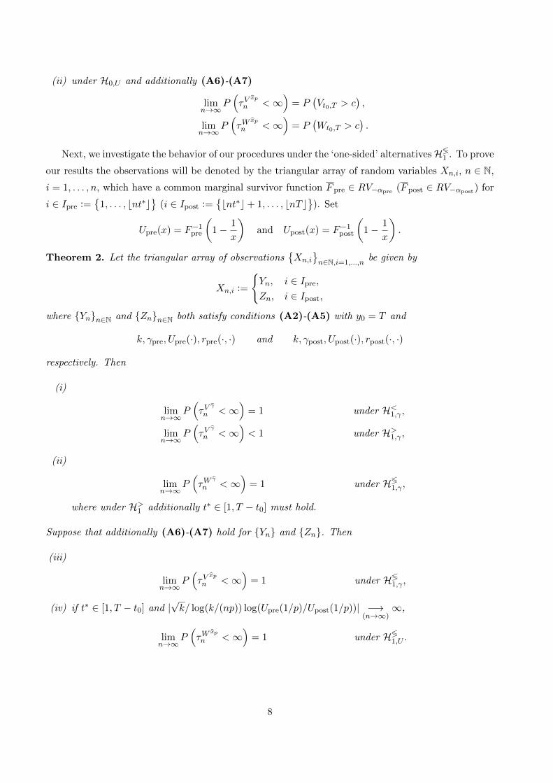
3 Simulations
In this section we investigate the finite-sample behavior of the monitoring procedures based on the
stopping times τWγ/xp
n and τVγ/xp
n . Throughout we simulate 10,000 time series with historical periods
of length n = 125, 500 and T = 4, such that the total length is bnT c = 500, 2000. Furthermore we
use t0 = 0.2 and k/n = 0.2 and the estimator γ = γH of the extreme value index we employ is the
Hill (1975) estimator. Simulation results were quite robust to the particular choice of k/n and are
available from the authors upon request. The quantiles of the distributions of Vt0,T and Wt0,T from
(10) are tabulated in Table 1 for t0 = 0.2 and T = 4. To simulate them we used 100,000 realizations
of Brownian motions on the interval [0, 4], which themselves were generated using 400,000 normally
distributed random variables.
αq 0.50 0.60 0.70 0.80 0.90 0.95 0.99αq-quantile of Vt0,T 78.35 113.0 166.2 257.8 464.5 723.4 1557αq-quantile of Wt0,T 15.57 18.42 22.10 27.39 36.79 46.87 72.89
Table 1: Quantiles of Vt0,T and Wt0,T (t0 = 0.2, T = 4)
X DGP Size bnT c = 500 bnT c = 2000
X γ X xp X γ X xp
p = 0.1 0.01 0.001 p = 0.1 0.01 0.001
V (ARMA) 10 5.4 11 7.7 6.0 7.1 10 8.7 7.95 2.7 6.2 4.0 3.0 3.6 5.5 4.5 3.7
(ARCH) 10 5.9 12 9.0 6.9 7.5 11 9.0 8.05 2.8 6.6 4.6 3.5 3.8 5.5 4.5 4.1
(SV) 10 8.0 11 10 9.2 8.5 10 10 9.35 4.3 5.9 6.0 5.3 4.3 5.5 5.1 4.6
W (ARMA) 10 15 8.4 11 14 10 8.6 8.8 9.75 8.8 4.4 6.7 8.3 5.5 4.4 4.7 4.9
(ARCH) 10 13 7.9 12 13 11 8.5 11 125 7.7 4.4 7.5 8.2 6.1 4.6 6.5 6.8
(SV) 10 16 8.7 15 16 10 8.2 10 115 11 5.2 10 11 5.8 4.0 5.7 5.9
Table 2: Empirical sizes in % of monitoring procedures based on X γ and X xp (X ∈ V,W) for bnT crealizations of (ARMA), (ARCH) and (SV)
We investigate size using data from a linear ARMA(1,1) and non-linear ARCH(1) and SV models.
11

X DGP t∗ Level bnT c = 500 bnT c = 2000
X γ X xp X γ X xp
p = 0.1 0.01 0.001 p = 0.1 0.01 0.001
V (ARMA) 1.15 10 7.4 96 66 33 9.7 100 97 755 3.4 92 53 23 4.5 100 94 62
2.5 10 18 81 57 38 40 100 95 825 11 70 45 27 27 98 89 71
(ARCH) 1.15 10 17 43 37 28 37 77 71 595 11 33 27 19 26 65 59 47
2.5 10 12 26 23 18 22 44 42 345 6.7 18 16 11 14 31 31 23
(SV) 1.15 10 27 73 57 45 83 99 97 945 15 58 40 29 69 97 91 85
2.5 10 8.5 28 15 11 22 72 46 365 3.6 17 7.4 5.0 11 57 32 22
W (ARMA) 1.15 10 20 54 41 32 22 98 80 585 13 41 31 23 14 95 68 45
2.5 10 18 45 31 25 19 97 70 475 11 33 22 17 12 92 57 34
(ARCH) 1.15 10 32 30 43 40 50 60 69 645 23 22 33 30 38 48 58 52
2.5 10 25 22 31 30 37 47 54 495 17 15 23 21 27 35 43 38
(SV) 1.15 10 0.9 10 1.5 0.8 6.1 54 26 165 0.4 5.3 0.6 0.0 2.2 38 14 7.8
2.5 10 10 11 9.7 10 10 48 25 185 6.2 5.6 5.9 6.1 4.9 33 14 9.2
Table 3: Empirical power in % of monitoring procedures based on X γ and X xp (X ∈ V,W) forbnT c realizations of (ARMA), (ARCH) and (SV)
Specifically, we simulate Xii=1,...,bnT c from the three data generating processes (DGPs)
Xi = 0.3 ·Xi−1 + Zi + 0.7 · Zi−1, Zii.i.d.∼ t10, (ARMA)
X2i =
(0.01 + 0.3125 ·X2
i−1
)Z2i , Zi
i.i.d.∼ N (0, 1), (ARCH)
|Xi| = σi|Zi|, Zii.i.d.∼ t0.5, (SV)
where tν denotes a Student’s t-distribution with ν degrees of freedom (i.e., tail index equal to ν) and
σi = 0.5σi−1 + εi, εi.i.d.∼ N (0, 1), a Gaussian AR(1)-process. For the verification of the conditions
(A2)-(A7) for the first two models we refer to Drees (2003, Secs. 3.1 & 3.2). The |Xi| generated from
the ARMA(1,1)-model have tail index 10 because of Lemma 5.2 in Datta and McCormick (1998).
The tail index of the X2i from the ARCH(1)-model is given by 8/2 = 4 (cf. Davis and Mikosch,
12

1998, Table 1), while that of |Xi| from (SV) is 0.5 (see Section 2.3). The parameters are chosen to
demonstrate that our procedure works well for tails ranging from rather light (in the (ARMA) case)
to very heavy with non-existent first moment (in the (SV) case).
The conclusions that can be drawn from Table 2 are quite similar for all models. When bnT c = 500
size varies around the nominal level quite a bit for different choices of p. This is no longer the case for
the longer period, where size is always very close to the expected level. Although we cannot offer any
intuition, it is interesting to observe that when the procedures based on the detectors V are oversized,
those based on W are undersized and vice versa.
To assess the power of our tests we generate data from the following models, where the historical
data in all three cases are generated according to the models already investigated under the null:
Xi,n =
0.3 ·Xi−1 + Zi + 0.7 · Zi−1, i = 1, . . . , bnt∗c ,0.8 ·Xi−1 + Zi + 0.7 · Zi−1, i = bnt∗c+ 1, . . . , bnT c ,
Zii.i.d.∼ t10, (15)
X2i,n =
(
0.01 + 0.3125 ·X2i−1
)Z2i , i = 1, . . . , bnt∗c ,(
0.01 + 0.5773 ·X2i−1
)Z2i , i = bnt∗c+ 1, . . . , bnT c ,
Zii.i.d.∼ N (0, 1), (16)
|Xi| = σi|Zi,n|, where Zi,n ∼
t0.5, i = 1, . . . , bnt∗c ,t1, i = bnt∗c+ 1, . . . , bnT c ,
(17)
where n = 125, 500 and T = 4 as before, t∗ = 1.15, 2.5, corresponding to breaks after 5% and 50%
of the observation period, and the Zi,n are independent. Here, i.ni.d. stands for independent, non-
identically distributed. In the ARMA(1,1)-model with the break in the AR-parameter from 0.3 to 0.8
there is no break in the tail index, but a break in the variance from 0.92 to 1.81, i.e., a more volatile
distribution after the break. In the ARCH case the parameter shift induces a tail index change from
8/2 = 4 to 4/2 = 2 (cf. Davis and Mikosch, 1998, Table 1), i.e., heavier tails after the break. At
the same time the variance is finite pre-break and (hairline) infinite post-break. For the stochastic
volatility model with the break in the error distribution the break is in the opposite direction with a
change in the tail index from 0.5 to 1.
Note that for the ARMA(1,1) model in (15) the null hypothesis H0,γ is true. However, as in finite
samples an upward break in the variance may not be clearly discerned from one in the tail index by our
procedure, we should expect more rejections for τV/W γ
n than in Table 2. This is generally confirmed
by the results in Table 3. Furthermore, the variance change is most frequently detected using τV/W xp
n
for p = 0.1. This may be explained by the higher variance of the estimates xp for smaller values of
p, which makes detection of a quantile break very difficult, if the quantiles do not lie sufficiently far
apart, as is plausible here, where a mere variance change occurred.
If there is a break in the tail index and the variance as in the ARCH- and SV-case, one can see
from Table 3 that the procedures based on the Weissman (1978) estimator clearly perform better than
those based solely on the Hill (1975) estimator. Heuristically, this may be explained by the fact that
the Weissman (1978) estimator also takes differences in scale before and after the break into account
13

Den
sity
1.0 1.5 2.0 2.5 3.0 3.5 4.0
0.0
0.5
1.0
1.5
2.0
(a1) τnXγ
for t*=1.15
Den
sity
1.0 1.5 2.0 2.5 3.0 3.5 4.0
01
23
4
(b1) τnXxp
for p=0.1 and t*=1.15
Den
sity
1.0 1.5 2.0 2.5 3.0 3.5 4.0
0.0
0.5
1.0
1.5
2.0
(c1) τnXxp
for p=0.001 and t*=1.15
Den
sity
1.0 1.5 2.0 2.5 3.0 3.5 4.0
0.0
0.5
1.0
1.5
(a2) τnXγ
for t*=2.5
Den
sity
1.0 1.5 2.0 2.5 3.0 3.5 4.0
0.0
1.0
2.0
3.0
(b2) τnXxp
for p=0.1 and t*=2.5
Den
sity
1.0 1.5 2.0 2.5 3.0 3.5 4.0
0.0
0.5
1.0
1.5
2.0
(c2) τnXxp
for p=0.001 and t*=2.5
Figure 1: Histograms of detection times τXγ
n , τXxp
n for X = V (blue) and for X = W (bright red) forp = 0.1, 0.001 for (15) and t∗ = 1.15 ((a1), (b1), (c1)), t∗ = 2.5 ((a2), (b2), (c2)) for bnT c = 2000
14

Den
sity
1.0 1.5 2.0 2.5 3.0 3.5 4.0
0.0
0.2
0.4
0.6
0.8
(a1) τnXγ
for t*=1.15
Den
sity
1.0 1.5 2.0 2.5 3.0 3.5 4.0
0.0
0.4
0.8
1.2
(b1) τnXxp
for p=0.1 and t*=1.15
Den
sity
1.0 1.5 2.0 2.5 3.0 3.5 4.0
0.0
0.4
0.8
(c1) τnXxp
for p=0.001 and t*=1.15
Den
sity
1.0 1.5 2.0 2.5 3.0 3.5 4.0
0.0
0.2
0.4
0.6
0.8
(a2) τnXγ
for t*=2.5
Den
sity
1.0 1.5 2.0 2.5 3.0 3.5 4.0
0.0
0.4
0.8
(b2) τnXxp
for p=0.1 and t*=2.5
Den
sity
1.0 1.5 2.0 2.5 3.0 3.5 4.0
0.0
0.5
1.0
1.5
2.0
(c2) τnXxp
for p=0.001 and t*=2.5
Figure 2: Histogram of detection times τXγ
n , τXxp
n for X = V (blue) and for X = W (bright red) forp = 0.1, 0.001 for (16) and t∗ = 1.15 ((a1), (b1), (c1)), t∗ = 2.5 ((a2), (b2), (c2)) for bnT c = 2000
15

(via Xk(s, t, 1); see (5)). Since in reality, changes in the tail index will most likely result in changes
of scale, one should use the tests based on V/W xp . Further, the choice τVxp
n with p = 0.1 leads to
the highest power, particularly for small sample lengths and the downward break in tail heaviness for
model (17).
Recall that the procedure based on V γ is inconsistent under H>1,γ . While this is not yet apparent
for the early break (t∗ = 1.15), it is for the late break (t∗ = 2.5), where power is significantly lower
as a larger portion of the sample upon which γ(1, t) is based is ‘contaminated’ by very heavy tailed
observations.
For sequential tests like ours, power is not the only criterion by which to judge a procedure, but
also how promptly changes are detected. To look into this, Figures 1 and 2 show histograms of the
(finite) realizations of τV/W γ
n and τV/W xp
n (bright blue / red) at the 10% level for the ARMA and the
ARCH models given in (15) and (16) respectively with bnT c = 2000. The histogram for (17) does not
provide any additional insights and is omitted. There are 19 bars in all plots with breaks at 1 + l ·0.15
(l = 1, . . . , 20). The value of t∗ at which the changes are located are given by 1.15 = 1+1 ·0.15 (l = 1)
and 2.5 = 1 + 10 · 0.15 (l = 10).
The results for the ARMA model are displayed in Figure 1. The high false detection rate for the
tail index-based method using the detector W γn seems largely to be due to false detections just shortly
after the break, as can be seen from the distinctive peaks in panels (a1) and (a2). The detections
with τWxp
n for p = 0.1 in (b1) and (b2) indicate that a very large portion of detections occur within
the time corresponding to the two bars right after the break. This holds to a lesser extent for the
results shown in (c1) and (c2), where, however, detection rates were poor. Overall the detection speed
is satisfactory but faster for larger values of p. For the ARCH model one can see slightly dissimilar
detection patterns for all procedures based on W . The highest number of detections always occurs one
or two bars after the break and that rate goes down only slowly so that detections (if they occur) take
on average longer than in the ARMA case. This may be explained by the fact that ARCH models
incorporate conditional heteroscedasticity, such that detection of changes in the variability of time
series is inherently more difficult. We need to observe longer periods of higher volatility before one
can reject the null here.
Comparing these results with those for the procedures based on V we see that for the latter
detections take much longer. They never peak in the initial period, where the change occurs. This
introduces a delicate trade-off for the detectors we introduced. The stopping times based on V
terminate more often under the alternative than those based on W , but they take longer to do so. So
if a swift detection is of the utmost importance, we recommend to use τWxp
n for p = 0.01. If it is more
important that a break is detected at all, but speed is of lesser interest, then τVxp
n for p = 0.01 seems
to be the wisest choice, unless a break towards lighter tails is expected in which case power was rather
dismal.
16

4 Application
In this section we apply our tests to the lower tail of log-returns, i.e., log-losses, of Bank of America
stocks covering the period of the financial crisis of 2007-2008, where short selling US financial stocks
was halted until October 2, 2008 following an SEC order released on September 19, 2008. The return
series we consider is displayed in the top part of Figure 4. Results for stock prices of other US
financial companies (Morgan Stanley, Citigroup and Goldman Sachs) are very similar and can be
obtained upon request. Since we try to detect changes in unconditional quantiles, our focus is on
the long-term distributional changes in the time series, not on short-term changes in the conditional
distribution. We set our (artificial) training and observation period to be the years from 2005 to
2012 corresponding to 2013 observations, X1, . . . , X2012, the first quarter of which (roughly the years
2005 and 2006) make up the training period. The lengths of the training and observation period were
chosen to correspond to the case n = 500 in the simulations, for which size and power proved to be
very satisfying. Furthermore, we choose the training period to precede the onset of the financial crisis
in 2007, so that we may analyze the performance of our procedures during these tumultuous years.
0 1 2 3 4 5
−4.
6−
4.4
−4.
2−
4.0
−3.
8−
3.6
−3.
4
−log(j/(n+1))
log
Xn−
j+1:
n
(a)
0 50 100 150 200
0.0
0.1
0.2
0.3
0.4
0.5
Number of order statistics k
Hill
est
imat
e
(b)
Figure 3: (a) Pareto quantile plot of shifted data. (b) Hill estimates as a function of upper orderstatistics k used in the estimation.
Given the very calm behavior of the log-returns during the training period one may have suspected
that a break toward heavier tails is much more likely than one toward lighter tails. Additionally, it
is vital for managing risk adequately to detect a break in the tail behavior quickly, because if it is
registered to late the cost of hedging that risk may already have increased dramatically. For these two
reasons we focus on the detectors W , which performed only slightly worse than the detectors V when
17

there is break leading to heavier tails, yet detected those much faster.
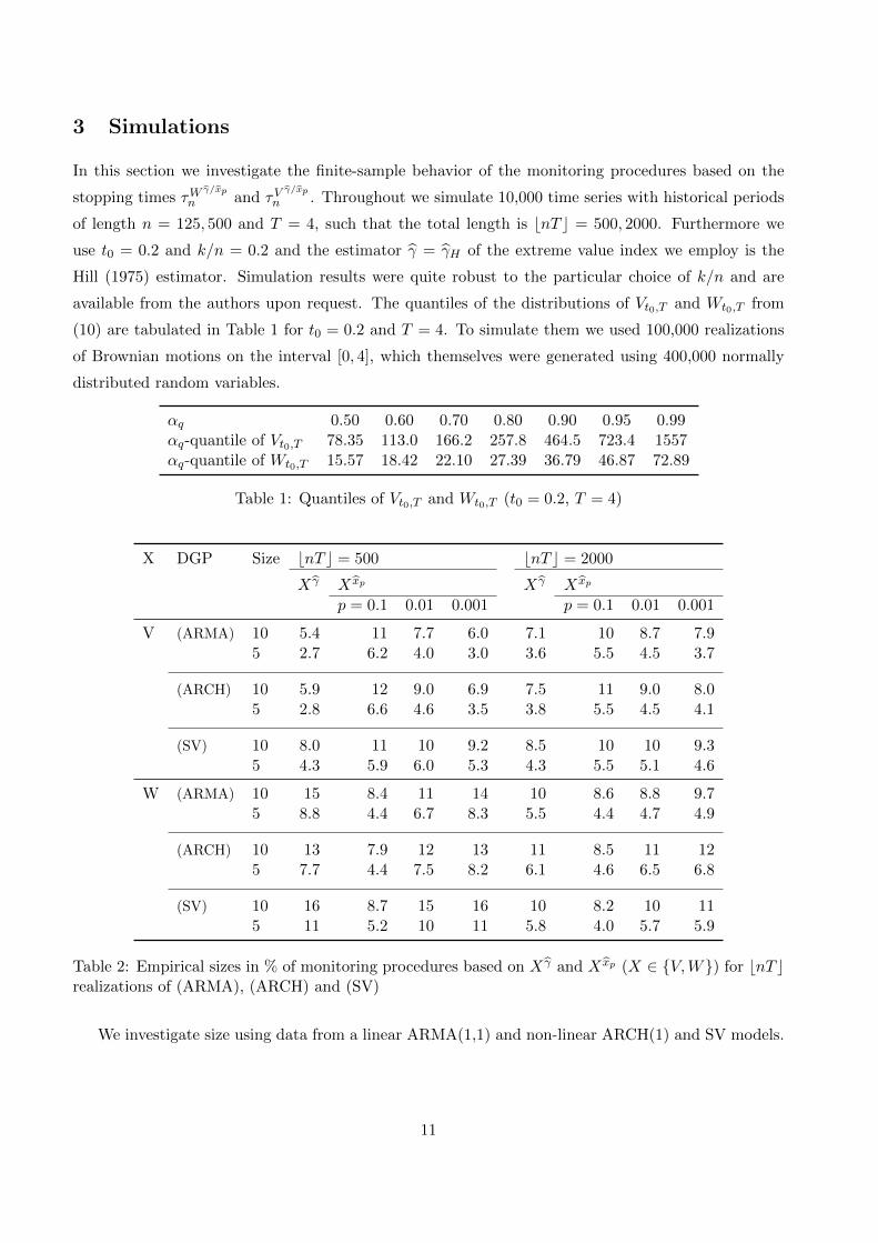
Next, we verify that our two central assumptions, the stationary mixing assumption (A2) and
the heavy tail assumption (A5), are plausibly met by the time series in the training period. To
check whether there is evidence for heavy tails we plot the Pareto quantile plot in Figure 3 (a), where
the points (− log(j/(n + 1)), logXn−j+1:n), j = 1, . . . , n, are plotted. See Beirlant, Vynckier and
Teugels (1996) for more on Pareto quantile plots. In order for all logXn−j+1:n’s to be well-defined
we shifted the observations to the positive half-line by adding the absolute value of the smallest
return plus 0.01. An upward sloping linear trend, like the one that can be seen in Figure 3 (a) from
− log(j/(n + 1)) ≈ 1.5 onwards, for some j = 1, . . . , k + 1 in the plot indicates a good fit of the
tail to (strict) Pareto behavior. An estimate of 1/α can then be obtained as the slope of the line
from the point (− log((k + 1)/(n+ 1)), logXn−k:n) onwards, where the slope seems to be roughly 0.2.
This is confirmed in the (slightly upward trending) Hill plot in Figure 3 (b), which displays the Hill
estimates of the shifted data as a function of the upper order statistics k used in the estimation.
As for the mixing assumption (A2) the best ARCH(p)-model (by AIC) was an ARCH(1). Using
an ARCH-LM test however, we could not reject the null of no conditional heteroscedasticity for this
model (p-value of 0.86). Routine testing and plotting of the autocorrelation function of the raw and
squared log-losses also revealed no dependence in the data, such that the data may reasonably be
regarded as independent. Further, applying the retrospective tests of Hoga (2016+) and Hoga (2015)
we found no evidence of extreme quantile or tail index breaks during that period which would violate
the stationarity assumption. Hence, we proceed with our monitoring procedure.
Since their inception by Engle (1982) (G)ARCH-models have arguably become the most popular
models for returns on risky assets. So the absence of ARCH-effects in the training period may be
surprising. However, Starica and Granger (2005) argue for models of returns that are locally i.i.d.
In our case the period from 2005 to 2006 seems to be a period, where returns behave like an i.i.d.
sequence.
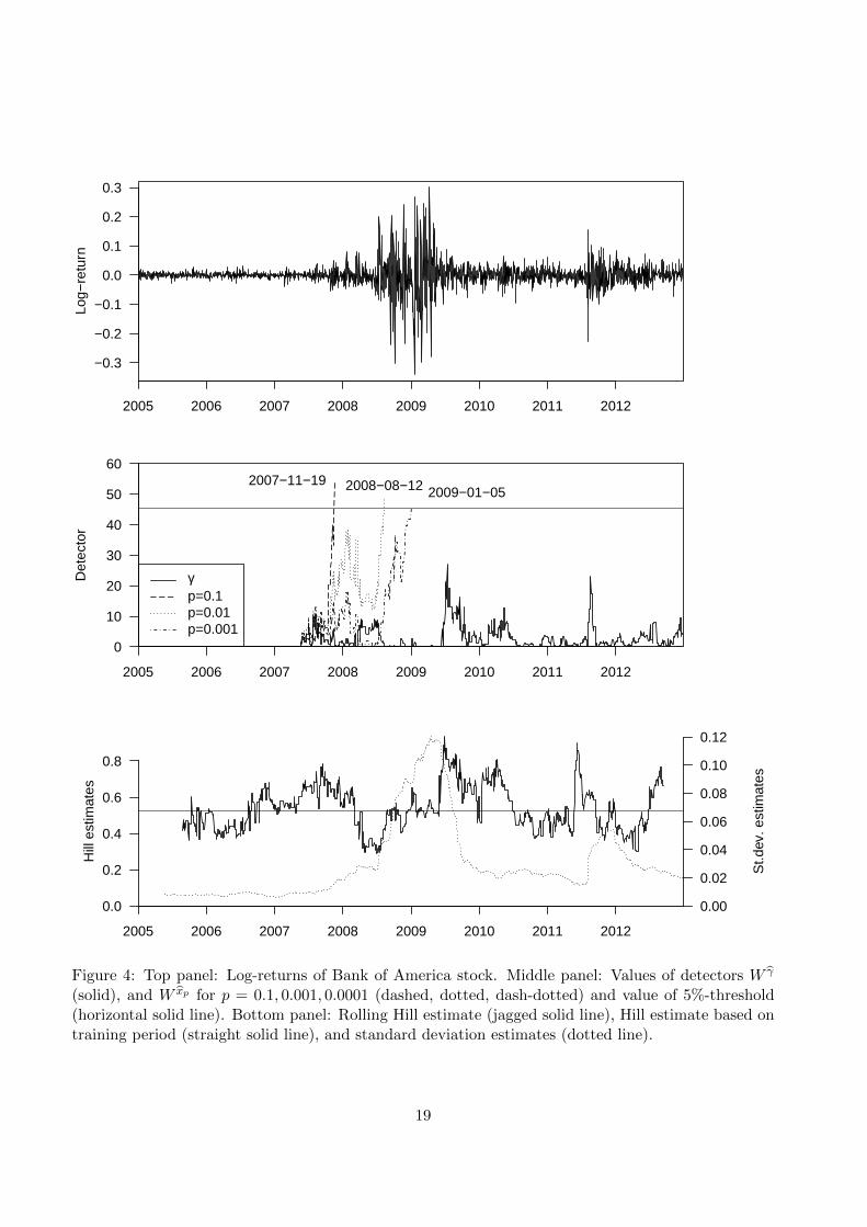
The results are shown in the middle part of Figure 4. As in the simulations we choose k/n = 0.2
and t0 = 0.2. All procedures terminate at the 5%-level if the value of 45.4 is exceeded by the detector.
We see that the procedure testing for a change in the 10%-quantile of the log-returns terminates first
in November of 2007, followed later by the detection of a break in the 1%-quantile in August 2008.
A 0.1%-quantile break is detected last in early 2009. However, we find no evidence of a tail index
break in the observation period. The lower part of Figure 4 sheds some light on this phenomenon.
There, the rolling window extreme value index estimates based on samples of length bnt0c = 100, that
the detectors are based on, are presented. The estimates hover around the value of 0.6 during the
whole period, which is roughly the extreme value index estimate of 0.52 based on the training period.
(Due to the location dependence of Hill estimates, the extreme value index in the training period was
estimated to be roughly 0.2 for the shifted data in Figure 3 (b) and 0.52 now, based on non-shifted
returns. The extreme value index itself is of course shift-invariant.) This contrasts with the behavior
18
−0.3
−0.2
−0.1
0.0
0.1
0.2
0.3
Log−
retu
rn
2005 2006 2007 2008 2009 2010 2011 2012
0
10
20
30
40
50
60
Det
ecto
r
γp=0.1p=0.01p=0.001
2005 2006 2007 2008 2009 2010 2011 2012
2007−11−19 2008−08−12 2009−01−05
0.0
0.2
0.4
0.6
0.8
Hill
est
imat
es
St.d
ev. e
stim
ates
0.00
0.02
0.04
0.06
0.08
0.10
0.12
2005 2006 2007 2008 2009 2010 2011 2012
Figure 4: Top panel: Log-returns of Bank of America stock. Middle panel: Values of detectors W γ
(solid), and W xp for p = 0.1, 0.001, 0.0001 (dashed, dotted, dash-dotted) and value of 5%-threshold(horizontal solid line). Bottom panel: Rolling Hill estimate (jagged solid line), Hill estimate based ontraining period (straight solid line), and standard deviation estimates (dotted line).
19

of the standard deviation estimates based on the same rolling windows, where we see a marked spike
peaking in early 2009. Hence, we find indications that the change in the extreme quantiles is not
caused by a change in the tail index but rather by a change in the scale of the log-returns. Largely,
the above results are consistent with the simulations under the alternative, where a variance change
occurred. Procedures based on W xp detect mere variance changes more easily for larger values of p,
while that based on W γ did not pick up a tail index change.
Appendix
Proof of Theorem 1: In the following let K,K1 be positive constants that may change from line
to line. The proof of (i) mainly rests on a time shifted version of the (weighted) weak convergence
established in Hoga (2016+, Theorem 5); see also the proof of Theorem 1 in Hoga (2016+). That is,
for any t0 > 0 we have that for some δ > 0 and any ν ∈[0, 1/2
),
1
yνen(t, y) :=
√k
yν
1
k
bntc∑i=1
[IUi>1− k
ny −
k
ny
] D−→(n→∞)
1
yνW (t, y) in D
([t0, T ]× [0, y0 + δ]
)(A.1)
for a sequence of uniformly distributed random variables Ui ∼ U [0, 1] satisfying (A2)-(A4), where
W (t, y) is a continuous centered Gaussian process with covariance function
Cov(W (t1, y1) ,W (t2, y2)
)= min (t1, t2) r (y1, y2)
and r(·, ·) defined in (A3). For the continuous mapping theorem (CMT) to imply (A.8) below, we
need to extend the convergence in (A.1) to D([0, T ]× [0, y0 + δ]
). To do so, it suffices to show by
Billingsley (1968, Thm. 4.2) that
limt0↓0
lim supn→∞
P
supt∈[0,t0]y∈(0,y0]
∣∣∣∣en(t, y)
yν
∣∣∣∣ > ε
=0, (A.2)
limt0↓0
P
supt∈[0,t0]y∈(0,y0]
∣∣∣∣W (t, y)
yν
∣∣∣∣ > ε
=0, (A.3)
where y0 := y0 + δ. We first show (A.3) by using the inequality in Lin and Choi (1999, Lem. 2.1)
similarly as in the proof of Hoga (2016+, Thm. 5). More specifically, we set
Dj := [0, t0]× [y0e−(j+1), y0e
−j ],
Γ2j := sup
t∈DjE[W (t, y)]2 = sup
t∈Djtr(y, y) ≤ Kt0y0e−(j+1),
λj := t0y0e−(j+1)[e− 1]
20
and use φ(r) := K√r. Then, Lemma 2.1 of Lin and Choi (1999) implies
P
supt∈[0,t0]y∈(0,y0]
∣∣∣∣W (t, y)
yν
∣∣∣∣ > ε
≤∞∑j=0
P
supt∈[0,t0]
y∈(y0e−(j+1),y0e−j]
∣∣W (t, y)∣∣ > ε
(y0e−(j+1)
)ν
≤ K∞∑j=0
1
t0y0e−(j+1)exp
−1
2
ε(y0e−(j+1)
)νΓj + (2
√2 + 2)K1
´∞0 ϕ(
√2λj2−x
2)dx
2
≤ Kt2ν
1−2ν
0
∞∑j=0
((t
11−2ν
0 y0e−(j+1)
)2ν−1) 1
1−2ν
exp
−K1
(t
11−2ν
0 y0e−(j+1)
)2ν−1−→(t0↓0)
0.
Before proving (A.2), put
Ss(y) :=1
yν1√k
s∑i=1
[IUi>1− k
ny −
k
ny
]and ‖Ss‖ := sup
y∈(0,y0]
∣∣Ss(y)∣∣ .
Now use the Ottaviani-type inequality from Bucher (2015, Lem. 3) to obtain
P
supt∈[0,t0]y∈(0,y0]
∣∣∣∣en(t, y)
yν
∣∣∣∣ > ε
= P
max
s=1,...,bnt0c‖Ss‖ > ε
≤
P∥∥∥Sbnt0c∥∥∥ > ε
+ P
maxr<s∈1,...,bnt0cs−r≤2rn
‖Ss − Sr‖ > ε
+ bnt0crn
β(rn)
1−maxs=1,...,bnt0c P∥∥∥Sbnt0c − Ss∥∥∥ > ε
. (A.4)
To start, consider the three terms in the numerator. First, bnt0crnβ(rn) tends to zero as n → ∞ by
(A2). Second, from (A.1) and the CMT,
P∥∥∥Sbnt0c∥∥∥ > ε
−→
(n→∞)P
sup
y∈(0,y0]
∣∣∣∣W (t0, y)
yν
∣∣∣∣ > ε
,
where the limit tends to zero as t0 ↓ 0 because of (A.3). Finally,
maxr<s∈1,...,bnt0c
s−r≤2rn
‖Ss − Sr‖ = maxr<s∈1,...,bnt0c
s−r≤2rn
supy∈(0,y0]
1
yν
∣∣∣∣∣∣ 1√k
s∑i=r+1
[IUi>1− k
ny −
k
ny
]∣∣∣∣∣∣≤ max
r<s∈1,...,bnt0cs−r≤2rn
supy∈(0,y0]
1
yν
∣∣∣∣∣∣ 1√k
s∑i=r+1
IUi>1− kny
∣∣∣∣∣∣+ supy∈(0,y0]
1
yν
∣∣∣∣2rn√k kny∣∣∣∣ =: An +Bn.
21
Bn tends to zero by (A2). As for An, we have
P An > ε ≤ P
max
m∈0,...,
⌊bnt0c2rn
⌋ supy∈(0,y0]
1
yν
∣∣∣∣∣∣∣1√k
b(m+2)2rnc∑i=bm2rnc+1
IUi>1− kny
∣∣∣∣∣∣∣ > ε
≤⌊bnt0c2rn
⌋P
supy∈(0,y0]
1
yν
∣∣∣∣∣∣ 1√k
4rn∑i=1
IUi>1− kny
∣∣∣∣∣∣ > ε
≤ t0K −→(t0↓0)
0, (A.5)
where we have used strict stationarity in the second to last inequality and a result from the proof of
Hoga (2016+, Thm. 5) in the last inequality. Thus, all terms in the numerator tend to zero.
We now turn to the denominator in (A.4) and show that it tends to one. Using strict stationarity
again, we get
maxs∈1,...,bnt0c
P∥∥∥Sbnt0c − Ss∥∥∥ > ε
= max
s∈1,...,bnt0cP‖Ss‖ > ε
= max
m∈1,...,bnt0cP
supy∈(0,y0]
1
yν
∣∣∣∣∣∣ 1√k
m∑i=1
[IUi>1− k
ny −
k
ny
]∣∣∣∣∣∣ > ε
.
Fix η > 0 small and set in := min
i ∈ N :
√k ≤ η
(y0e−(i+1)
)ν−1. Decompose
1
yν1√k
m∑i=1
[IUi>1− k
ny −
k
ny
]=
1
yν
bm/rnc−1∑w=0
1√k
(w+1)rn∑i=rn+1
[IUi>1− k
ny −
k
ny
]
+1
yν1√k
m∑i=bm/rncrn+1
[IUi>1− k
ny −
k
ny
]. (A.6)
The second-term on the right-hand side of (A.6) contains at most rn terms and hence its supremum
can be bounded by
supy∈(0,y0]
1
yν1√k
m∑i=bm/rncrn+1
IUi>1− kny +
rn√k
k
ny1−ν0 =: An + Bn.
Clearly, Bn = o(1) and that An = oP (1) can be seen as for An in (A.5).
To show that the first term on the right-hand side of (A.6) is oP (1) it suffices to do so for
Smn , where mn =⌊m2rn
⌋, Smn := 1
yν∑mn
j=1 Yn,j with Yn,j an i.i.d. stochastic process distributed
as 1√k
∑rni=1
[IUi>1− k
ny −
kny
]; see the proof of Drees (2000, Thm. 2.3).
Then, following the derivations in Drees (2000, Eq. (5.6)) leads to
P
sup
y∈(0,y0e−in ]
∣∣∣Smn(y)∣∣∣ > ε
≤ Kη −→
(η→0)0,
where K is independent of m. It remains to prove
P
sup
y∈(y0e−in ,y0]
∣∣∣Smn(y)∣∣∣ > ε
−→
(n→∞)0.
22
By condition (A4) for the Ui we have E[Yn,1(y)− Yn,1(y)
]j ≤ Crn knk−j/2(y−x), whence Burkholder’s
inequality implies
E
[yν(Smn(y)− Smn(x)
)]4≤ K
mn E
[Yn,1(y)− Yn,1(x)
]4+mn(mn − 1)
E[Yn,1(y)− Yn,1(x)
]22
≤ K
m
n
1
k(y − x) +
(m
n
)2
(y − x)2
.
Hence, we obtain as in the proof of Drees (2000, Thm. 2.3) that
P
sup
y∈(y0e−in ,y0]
∣∣∣∣∣ Smn(y)
yν
∣∣∣∣∣ > ε
≤(m
n
)2
K
in−1∑i=0
(y0e−i)2
[y0e−(i+1)
]−4ν≤(m
n
)2
K
ˆ y0/e
0u1−νdu ≤ Kt20 −→
(t0↓0)0,
finishing the proof of (A.2). Combining (A.1), (A.2) and (A.3) gives
√k
yν
1
k
bntc∑i=1
[IUi>1− k
ny −
k
ny
] D−→(n→∞)
1
yνW (t, y) in D
([0, T ]× [0, y0 + δ]
). (A.7)
Then for Xi satisfying (A2)-(A5), by the proof of Theorem 3.1 in Drees (2000), the uniformly
distributed Ui := F (Xi) satisfy (A2)-(A4) and
Xi > U
(n
ky
)⇐⇒ Ui > 1− k
ny.
Hence, from (A.7),
√k
yν
1
k
bntc∑i=1
IXi>U
(nky
) − ty D−→
(n→∞)
1
yνW (t, y) in D
([0, T ]× [0, y0 + δ]
)The CMT then implies
√k
yν
1k
∑bnmax(1+t0,t)ci=n+1 I
Xi>U(nky
) − (max(1 + t0, t)− 1)y
1k
∑bntci=bn(t−t0)c+1
IXi>U
(nky
) − t0y1k
∑bntci=1 I
Xi>U
(nky
) − ty
D−→
(n→∞)
1
yν
W (max(1 + t0, t), y)−W (1, y)W (t, y)−W (t− t0, y)
W (t, y)
in D3([t0, T ]× [0, y0 + δ]
). (A.8)
23

Now invoking a Skorohod construction (e.g., Wichura, 1970, Thm. 1) we get on a suitable probability
space
supt∈[t0,T ]
y∈(0,y0+δ]
1
yν
∣∣∣∣∣∣∣∣∣∣∣∣∣∣√k
1k
∑bnmax(1+t0,t)ci=n+1 I
Xi>U(nky
) − (max(1 + t0, t)− 1)y
1k
∑bntci=bn(t−t0)c+1
IXi>U
(nky
) − t0y1k
∑bntci=1 I
Xi>U
(nky
) − ty
−
W (max(1 + t0, t), y)−W (1, y)W (t, y)−W (t− t0, y)
W (t, y)
∣∣∣∣∣∣∣∣
a.s.−→(n→∞)
0.
Arguing component-wise as in the proof of Einmahl et al. (2016, Cor. 3) this implies for some δ > 0
(using the second-order condition (A5))
supt∈[t0,T ]
y≥y−1/γ0 −δ
yν/γ
∣∣∣∣∣∣∣∣∣∣∣∣√k
1k
∑bnmax(1+t0,t)ci=n+1 I
Xi>yU(nk ) − (max(1 + t0, t)− 1)y−1/γ
1k
∑bntci=bn(t−t0)c+1
IXi>yU(nk )
− t0y−1/γ1k
∑bntci=1 I
Xi>yU(nk )
− ty−1/γ
−
W (max(1 + t0, t), y−1/γ)−W (1, y−1/γ)
W (t, y−1/γ)−W (t− t0, y−1/γ)
W (t, y−1/γ)
∣∣∣∣∣∣∣∣
a.s.−→(n→∞)
0, (A.9)
where Hoga (2016+, Prop. 2) justifies the final step of their proof in our case. Now retrace the proof
of Hoga (2016+, Cor. 1) to see that
supt∈[t0,T ]y≥y−1/γ
0
yν/γ
∣∣∣∣∣∣∣∣∣∣∣√k
1k
∑bnmax(1+t0,t)ci=n+1 IXi>yXk(1,max(1+t0,t),1) − (max(1 + t0, t)− 1)y−1/γ
1k
∑bntci=bn(t−t0)c+1
IXi>yXk(t−t0,t,1) − t0y−1/γ
1k
∑bntci=1 IXi>yXk(0,t,1) − ty
−1/γ
−
W (max(1 + t0, t), y−1/γ)−W (1, y−1/γ)− y−1/γ
[W (max(1 + t0, t), 1)−W (1, 1)
]W (t, y−1/γ)−W (t− t0, y−1/γ)− y−1/γ
[W (t, 1)−W (t− t0, 1)
]W (t, y−1/γ)− y−1/γW (t, 1)
∣∣∣∣∣∣∣∣
a.s.−→(n→∞)
0.
(A.10)
The key ingredient in this step justifying the replacement of U(n/k) in (A.9) by the respective
Xk(s, t, 1) in (A.10) is the generalized Vervaat lemma in Einmahl et al. (2010, Lem. 5), which gives a
weak convergence result for Xk(0, t, 1)/U(n/k) from the third component of (A.9) (and similarly for
the other components). The convergence in (A.10) is the key result with which one may deduce weak
convergence results for various tail index estimators; see Examples 3 - 5 in Hoga (2016+). As already
24

mentioned, we focus here on the Hill estimator γ := γH defined in (6). Focus on the third component
of (A.10) (the others can be dealt with similarly) and notice that for j = 0, 1, . . . , bktc − 1
1
bktc
bntc∑i=1
IXi>yXk(0,t,1) =
bktc−jbktc , y ∈
[Xbntc−bktc+j:bntcXbntc−bktc:bntc
,Xbntc−bktc+j+1:bntcXbntc−bktc:bntc
),
0, y ≥ Xbntc:bntcXbntc−bktc:bntc
.
Then it is an easy exercise in integration to check that
√k(γH(0, t)− γ
)=√k
ˆ ∞1
1
bktc
bntc∑i=1
IXi>yXk(0,t,1) − y−1/γ
dy
y.
Similar representations hold for γ(1,max(1 + t0, t)) and γ(t− t0, t), so that (A.10) implies
√k
(max(1 + t0, t)− 1)(γ(1,max(1 + t0, t))− γ
)t0(γ(t− t0, t)− γ
)t(γ(0, t)− γ
) D−→
(n→∞)σγ,γ
W (max(1 + t0, t))−W (1)W (t)−W (t− t0)
W (t)
(A.11)
in D3[t0, T ], where σ2γ,γ = γ2´ 10
´ 10
r(x,y)xy −
r(x,1)x − r(1,y)
y + r(x, y)
dxdy and W (·) a standard Brow-
nian motion. Notice for this that by calculating covariancesˆ ∞1
[W (t, y−1/γ)− y−1/γW (t, 1)
] dy
y= γ
ˆ 1
0
[W (t, u)− uW (t, 1)
] du
u
D= σγ,γW (t).
From (A.11) and the CMT we obtain
V γn (t)
D−→(n→∞)
[W (t)− tW (1)
]2´ 1t0
[W (s)− sW (1)
]2ds
in D[1 + t0, T ], (A.12)
W γn (t)
D−→(n→∞)
[W (t)−W (t− t0)− t0W (1)
]2´ 1t0
[W (s)−W (s− t0)− t0W (1)
]2ds
in D[1 + t0, T ].
The result is now proved via another application of the CMT.
For part (ii) we observe that it follows from (A.11) similarly as in the proof of Theorem 1 in Hoga
(2015) that (for the general idea of how to derive convergence of xp from that of γ see (A.17) below
and the steps following it, in particular (A.18))
√k
log(k/(np)
)
(max(1 + t0, t)− 1) log(xp(1,max(1+t0,t))
U(1/p)
)t0 log
(xp(t−t0,t)U(1/p)
)t log
(xp(0,t)U(1/p)
)
D−→(n→∞)
σγ,γ
W (max(1 + t0, t))−W (1)W (t)−W (t− t0)
W (1)
in D3[t0, T ], (A.13)
whence with the CMT again
Vxpn (t)
D−→(n→∞)
[W (t)− tW (1)
]2´ 1t0
[W (s)− sW (1)
]2ds
in D[1 + t0, T ],
Wxpn (t)
D−→(n→∞)
[W (t)−W (t− t0)− t0W (1)
]2´ 1t0
[W (s)−W (s− t0)− t0W (1)
]2ds
in D[1 + t0, T ].
The conclusion follows as before.
25

Proof of Theorem 2: We first prove the two statements in (i). Under H>1,γ we get by an adaptation
of the proof of Hoga (2016+, Thm. 3) similar to the one in the proof of Theorem 1
√k(γ(1, t)− γpre
) D−→(n→∞)
Bpre(t)−Bpre(1)
t− 1in D [1 + t0, T ] (A.14)
and by a further close inspection that even
√k
(γ(1,max(1 + t0, t))− γpre
γ(0, t)− γpre
)D−→
(n→∞)
((Bpre(max(1 + t0, t))−Bpre(1))/(max(1 + t0, t)− 1)
Bpre(t)/t
)(A.15)
jointly in D2[t0, T ], where, setting tmin = min(t, t∗),
Bpre(t) = γpre
ˆ 1
0
[Wpre(tmin, u
t
tmin)− uWpre(tmin,
t
tmin)
]du
u
and Wpre(·, ·) is as W (·, ·) in (A.1) with r(·, ·) replaced by rpre(·, ·). Hence, (A.12) holds with W (·)replaced by Bpre(·), where Bpre(·) is also a continuous centered Gaussian process. The result follows.
For the other part of (i) it suffices to note that
γ(0, 1)P−→
(n→∞)γpre < γpost
P←−(n→∞)
γ(1, T ),
because by (A.14) γ will converge in probability to the dominant tail index (i.e., max(γpre, γpost)) in
a sample with one tail index break.
For (ii) simply note that
γ(0, 1)P−→
(n→∞)γpre < γpost
P←−(n→∞)
γ(t∗, t∗ + t0).
If γpre > γpost in (iii) (the other case is similar) we can deduce from (A.13) that√k
log(k/(np)
) log
(xp(0, 1)
Upre(1/p)
)= OP (1), and
√k
log(k/(np)
) log
(xp(1, T )
Upre(1/p)
(T
t∗
)γpre)= OP (1).
From this the result follows if we can establish the right-hand side result, because
Vxpn (T ) =
[(T − 1)
√k
log(k/(np))
log(
xp(1,T )Upre(1/p)
)− log
(xp(0,1)Upre(1/p)
)]2´ 1t0
[s
√k
log(k/(np)) log(xp(0,s)xp(0,1)
)]2ds
. (A.16)
Decompose(t
tmin
)γprexp(1, t)− Upre
(1
p
)=
[(t
tmin
)γpreXk(1, t, 1)− Upre
(n
k
)](np
k
)−γ(1,t)+
[(np
k
)−γ(1,t)−(np
k
)−γpre]Upre
(n
k
)
+
[Upre
(n
k
)(np
k
)−γpre− Upre
(1
p
)]=I + II + III. (A.17)
26

Before considering these three terms separately, observe that by the mean value theorem, using
∂∂τ (xτ ) = xτ log (x), there exists a ξ ∈ [−1, 1] such that(
np
k
)−γ(1,t)−(np
k
)−γpre=(−γ(1, t) + γpre
)(npk
)−γpre+ξ(γpre−γ(1,t))log
(np
k
)=
(np
k
)−γpre (γpre − γ(1, t)
)(npk
)ξ(γpre−γ(1,t))log
(np
k
).
Then use(np
k
)ξ(γpre−γ(1,t))= exp
[ξ(γpre − γ(1, t)
)log
(np
k
)]= exp
[ξOP
(1√k
)log
(np
k
)]P−→
(n→∞)1
uniformly in t (by (A6) and (A.14)) and (A7) to get
Upre
(nk
)Upre
(1p
) [(npk
)−γ(1,t)−(np
k
)−γpre]=Upre
(nk
)Upre
(1p
)(np
k
)−γpre (γpre − γ(1, t)
)(npk
)ξ(γpre−γ(1,t))log
(np
k
)=(1 + oP (1)
) (γpre − γ(1, t)
)log
(np
k
). (A.18)
Furthermore applying the functional delta method (e.g., van der Vaart and Wellner, 1996, Theo-
rem 3.9.4) to (a slight adaptation of) Hoga (2016+, Eq. (70)) yields
√k
Xk(1, t, 1)
Upre
(nk
) − ( t
tmin
)−γpreD−→
(n→∞)
− γpre(
t
tmin
)−(γpre+1)
Wpre
(tmin,
ttmin
)tmin
−Wpre
(1,
t
tmin
) in D[1 + t0, T ], (A.19)
where we used that
φ : D[1 + t0, T ]→ D[1 + t0, T ], φ(f(·)) = f−γpre(·)
is Hadamard-differentiable tangentially to C[1 + t0, T ] in t/tmin with derivative
φ′t/tmin(f(·)) = −γpre
(t
tmin
)−(γpre+1)
f(·).
27

Combining we get
I
Upre(1/p) log(knp
)=
1
Upre
(1p
) (npk
)−γ(1,t) 1
log(knp
) [Xk(1, t, 1)− Upre
(n
k
)]
=Upre
(nk
)Upre
(1p
) [(npk
)−γ(1,t)−(np
k
)−γpre+
(np
k
)−γpre] 1
log(knp
) [Xk(1, t, 1)
Upre
(nk
) − 1
]
(A7)=
(A.18)
[(1 + oP (1))(γpre − γ(1, t)) log
(np
k
)+ 1 + o
(1√k
)]1
log(knp
) [Xk(1, t, 1)
Upre
(nk
) − 1
]
(A.19)=
[(1 + oP (1))
√k(γpre − γ(1, t))k−1/2 log
(np
k
)+ 1 + o
(1√k
)]1
log(knp
)OP (1/√k)
(A6)=
(A.14)oP
(1/√k)
uniformly in t. Further, utilizing (A6) and (A7) for the third term,
III
Upre(1/p) log(knp
) =1
log(knp
) Upre
(nk
)Upre
(1p
) (npk
)−γpre − 1
= o(
1/√k).
Using (A.18) and (A.14) we get for the last term
(t− 1)√k
II
Upre
(1p
)log(knp
) D−→(n→∞)
Bpre(t)−Bpre(1) in D [1 + t0, T ] ,
whence
(t− 1)√k
log(knp
)(
ttmin
)γprexp(1, t)
Upre
(1p
) − 1
D−→(n→∞)
Bpre(t)−Bpre(1) in D [1 + t0, T ] .
Part (iv) is trivial, since√k
log(k/(np)
) log
(xp(0, 1)
Upre(1/p)
)= OP (1),
√k
log(k/(np)
) log
(xp(t
∗, t∗ + t0)
Upost(1/p)
)= OP (1).
The result follows using a similar expansion as in (A.16).
References
Asai M, McAleer M, Yu J. 2006. Multivariate stochastic volatility: A review. Econometric Reviews 25: 145–175.
Aschersleben P, Wagner M, Wied D. 2015. Monitoring euro area real exchange rates. In Steland A, Rafaj lowicz E,Szajowski K (eds.) Springer Proceedings in Mathematics and Statistics 122 (12th Workshop on Stochastic Models,Statistics and Their Applications), New York: Springer, pages 363–370.
Aue A, Hormann S, Horvath L, Huskova M, Steinebach J. 2012. Sequential testing for the stability of high-frequencyportfolio betas. Econometric Theory 28: 804–837.
Beirlant J, Goegebeur Y, Segers J, Teugels J. 2004. Statistics of Extremes. Chichester: Wiley.
28

Beirlant J, Vynckier P, Teugels J. 1996. Tail index estimation, Pareto quantile plots, and regression diagnostics. Journalof the American Statistical Association 91: 1659–1667.
Billingsley P. 1968. Convergence of Probability Measures. New York: Wiley.
Bradley R. 1986. Basic properties of strong mixing conditions. In Eberlein E, Taqqu M (eds.) Dependence in Probabilityand Statistics, Boston: Birkhauser, pages 165–192.
Bradley R. 2007. Introduction to strong mixing conditions Vol. I. Heber City: Kendrick Press.
Breiman L. 1965. On some limit theorems similar to the arc-sine law. Theory of Probability and its Applications 10:351–360.
Bucher A. 2015. A note on weak convergence of the sequential multivariate empirical process under strong mixing.Journal of Theoretical Probability 28: 1028–1037.
Chu JS, Stinchcombe M, White H. 1996. Monitoring structural change. Econometrica 64: 1045–1065.
Csorgo S, Viharos L. 1998. Estimating the tail index. In Szyszkowicz B (ed.) Asymptotic Methods in Probability andStatistics, Amsterdam: Elsevier, pages 833–881.
Danıelsson J, Jansen D, de Vries C. 1996. The method of moments ratio estimator for the tail shape parameter. Com-munications in Statistics - Theory and Methods 25: 711–720.
Datta S, McCormick W. 1998. Inference for the tail parameter of a linear process with heavy tail innovations. Annals ofthe Institute of Statistical Mathematics 50: 337–359.
Davis R, Mikosch T. 1998. The sample autocorrelatios of heavy-tailed processes with applications to ARCH. The Annalsof Statistics 26: 2049–2080.
de Haan L, Ferreira A. 2006. Extreme Value Theory. New York: Springer.
Dierckx G, Teugels J. 2010. Change point analysis of extreme values. Environmetrics 21: 661–686.
Drees H. 2000. Weighted approximations of tail processes for β-mixing random variables. The Annals of Applied Proba-bility 10: 1274–1301.
Drees H. 2003. Extreme quantile estimation for dependent data, with applications to finance. Bernoulli 9: 617–657.
Einmahl J, de Haan L, Zhou C. 2016. Statistics of heteroscedastic extremes. Journal of the Royal Statistical Society:Series B 78: 31–51.
Einmahl J, Gantner M, Sawitzki G. 2010. Asymptotics of the shorth plot. Journal of Statistical Planning and Inference140: 3003–3012.
Engle R. 1982. Autoregressive conditional heteroscedasticity with estimates of the variance of United Kingdom inflation.Econometrica 50: 987–1007.
Hill B. 1975. A simple general approach to inference about the tail of a distribution. The Annals of Statistics 3: 1163–1174.
Hill J. 2011. Extremal memory of stochastic volatility with an application to tail shape inference. Journal of StatisticalPlanning and Inference 141: 663–676.
Hoga Y. 2015. Testing for changes in (extreme) VaR. submitted to Econometrics Journal .
Hoga Y. 2016+. Change point tests for the tail index of β-mixing random variables. forthcoming in Econometric Theory .
Kelly B, Jiang H. 2014. Tail risk and asset prices. Review of Financial Studies 27: 2841–2871.
Kim M, Lee S. 2011. Change point test for tail index for dependent data. Metrika 74: 297–311.
Kulik R, Soulier P. 2011. The tail empirical process for long memory stochastic volatility sequences. Stochastic Processesand their Applications 121: 109–134.
Lin Z, Choi YK. 1999. Some limit theorems for fractional Levy Brownian fields. Stochastic Processes and their Applications82: 229–244.
Quintos C, Fan Z, Phillips P. 2001. Structural change tests in tail behaviour and the Asian crisis. Review of EconomicStudies 68: 633–663.
Resnick S. 2007. Heavy-Tail Phenomena: Probabilistic and Statistical Modeling. New York: Springer.
Shao X, Zhang X. 2010. Testing for change points in time series. Journal of the American Statistical Association 105:1228–1240.
Starica C, Granger C. 2005. Nonstationarities in stock returns. The Review of Economics and Statistics 87: 503–522.
van der Vaart A, Wellner J. 1996. Weak Convergence and Empirical Processes. New York: Springer.
Weissman I. 1978. Estimation of parameters and large quantiles based on the k largest observations. Journal of theAmerican Statistical Association 73: 812–815.
Wichura MJ. 1970. On the construction of almost uniformly convergent random variables with given weakly convergentimage laws. The Annals of Mathematical Statistics 41: 284–291.
Wied D, Galeano P. 2013. Monitoring correlation change in a sequence of random variables. Journal of Statistical Planningand Inference 143: 186–196.
Zeileis A, Leisch F, Kleiber C, Hornik K. 2005. Monitoring structural change in dynamic econometric models. Journalof Applied Econometrics 20: 99–121.
29