sequencing and tabu search heuristics for hybrid flow ...werner/t3d1.pdf · sequencing and tabu...

Proceedings of the 7th Asia Pacific Industrial Engineering and Management Systems Conference 2006 17-20 December 2006, Bangkok, Thailand

________________________________________ †: Corresponding Author

Sequencing and Tabu Search Heuristics for Hybrid Flow Shops with Unrelated Parallel Machines and Setup Times

Jitti Jungwattanakit†, Manop Reodecha, Paveena Chaovalitwongse Department of Industrial Engineering, Faculty of Engineering

Chulalongkorn University, Bangkok 10330 Thailand +662-218-6855, Email: [email protected].

Frank Werner

Faculty of Mathematics Otto-von-Guericke-University, P.O. Box 4120, D-39016 Magdeburg, Germany

Phone: +49-391-6712025, fax: +49-391-6711171, Email: [email protected]

Abstract. The goal of this paper is to investigate scheduling heuristics to seek the minimum of a positively weighted convex sum of makespan and the number of tardy jobs in a static hybrid flow shop environment where at least one production stage is made up of unrelated parallel machines. In addition, sequence - and machine - dependent setup times are considered. The problem is a combinatorial optimization problem which is too difficult to be solved optimally for large problem sizes, and hence heuristics are used to obtain good solutions in a reasonable time. Some dispatching rules and flow shop makespan heuristics are developed. Then this solution may be improved by fast polynomial heuristic improvement algorithms based on shift moves and pairwise interchanges. In addition, metaheuristic proposed is a tabu search algorithm. Three basic parameters (i.e., number of neighbors, neighborhood structure, and size of tabu list in each iteration) of a tabu search algorithm are briefly discussed in this paper. The performance of the heuristics is compared relative to each other on a set of test problems with up to 50 jobs and 20 stages. Keywords: Hybrid flow shop scheduling; Unrelated parallel machines; Setup times; Constructive algorithms; Improvement heuristics; Tabu Search algorithm.

1. INTRODUCTION Industrial scheduling presents a complex decision-

making scenario. Operations managers are confronted with the tough task to find an optimal solution from the large number of possible combinations that should be considered. This type of problem is also related to combinatorial optimization and NP-hardness, and consequently the search for efficient methods providing a good feasible solution continues to be a challenge. Once efficient algorithm methods are found, computational tools can be built that will allow managers to make rapid decisions with flexibility and efficiency.

This article has been concerned with heuristics to provide good and quick feasible solutions. They obtain solutions to large problems with limited computational effort. The heuristics concerned in this paper can be classified into two types; constructive (conventional) and iterative (modern) heuristic algorithms.

In a constructive algorithm, single or several solutions

are generated, but the only best one is chosen as the final solution. In this paper, several simple dispatching rules and flow shop heuristics are adapted to find a solution for the problem. Additionally, we investigate how to improve the quality of the solution by using several fast polynomial improvement algorithms.

The interest in iterative algorithms is due to the difficulty of solving real large-size problems by using an exact algorithm, while such metaheuristic algorithms can treat large complex problems and for this reason, they have got a considerable research attention over the last decades. This study will limit to one of the popular iterative algorithms known as a Tabu Search (TS) algorithm. It is originally proposed by Glover (1986). The TS algorithm is among the most cited and used metaheuristics for the combinatorial problems (Blum and Roli 2003). It has been successfully applied in a lot of different areas: scheduling, transportation, telecommunications, layout and circuit design, graphs, expert systems, and so on (see Glover and Laguna 1993 for a survey).

1330

Jungwattanakit et al.

Hence, in this paper TS-based algorithms will be used to solve the problem of scheduling a given set of n jobs at k stages on m unrelated parallel machines. Such a problem occurs in real world problems such as e.g. in the textile industry.

A textile manufacturer supervises workers who make products that contain fibers, such as clothing, tires, and yarn. Whatever the industry, the task of a textile manufacturer is the same: to convert raw products into usable goods. Typically, a textile production unit can hardly fit in any classical scheduling model. Instead, such a production unit is characterized by a multi-stage manufacturing process with multiple production units per stage (i.e., parallel machines), which makes production management quite complex. This combined model is referred to as the hybrid flow shop (HFS) or flexible flow shop (FFS) problem as shown in Figure 1. It can be noted that this problem is also known as the flow shop problem because the process follows a flow shop characteristic, but there are some processing stages having parallel machines to increase the overall capacities, to balance the capacities of the stages, or either to eliminate or reduce the impact of bottleneck stages on the overall shop floor capacities. Most textile companies are ageing while the technology changes rapidly. It is common to find newer or more modern machines running side by side with older and less efficient machines. Hence, these companies own machines of different ages, which may perform the same operations as the newer ones, but would generally require a longer operating time for the same operation.

Figure 1: A general schematic of the hybrid flow shop.

Sequence-dependent setup times and costs incur when

machines often have to be reconfigured or cleaned between jobs. This process is known as a changeover or setup. If the length of the setup depends on the job just completed and on the one about to be started, then the setup times are sequence-dependent. For instance, in the weaving phase the setup times are depending on the types of clothes being processed in sequence. Another example is dying operations which often require setups. Every time a new

color is used, the painting devices must be cleaned. The cleanup time often depends on the color just used as well as the color about to be used. Such a resection is called a sequence-dependent setup time.

For the past three decades, the hybrid flow shop scheduling problem has attracted many researchers. Numerous research articles have been published on this topic (see e.g. Wang 2005). There are two main reasons for this, among many others. Firstly, a hybrid flow shop environment is a category of machine scheduling problems which is difficult to solve (Garey and Johnson 1979; Gupta 1971). Thus, it is unlikely that polynomial time algorithms exist for the exact solution of the general problem. Secondly, this type of machine scheduling problem can find many real-world applications.

Although the hybrid flow shop problem has been widely studied in the literature, most of the studies related to hybrid flow shop problems concentrate on problems with identical processors, see for instance, Gupta, Krüger, Lauff, Werner and Sotskov (2002), Alisantoso, Khoo, and Jiang (2003), Lin and Liao (2003), and Wang and Hunsucker (2003). In this paper, however, the hybrid flow shop problem with unrelated non-identical parallel machines and sequence-dependent setup times is considered. This complex problem, which is encountered by many industries, is very difficult to solve.

Consequently, in this paper the hybrid flow shop with unrelated parallel machines like the textile industry will be solved by using some constructive and TS-based algorithms. The rest of this paper is organized as follows: The problem considered in this paper is described in Section 2. Some heuristic algorithms are proposed in Section 3. A TS algorithm is presented in Section 4. Computational results and conclusions are shown in Section 5 and Section 6, respectively.

2. STATEMENT OF THE PROBLEM The hybrid flow shop system is defined by a set O =

{1,…, t,…, k} of k processing stages. At each stage t, t ∈ O, there is a set Mt = {1,…, i,…, mt} of mt unrelated machines. The set J = {1,…, j,…, n} of n independent jobs has to be processed on machine of set M1,…, Mk. Each job j, j ∈ J, has its release date rj ≥ 0 and a due date dj ≥ 0. It has its fixed standard processing time for every stage t, t ∈ O. Owing to the unrelated machines, the processing time pt

ij of job j on machine i at stage t is equal to pst

j/ vtij, where pst

j is the standard processing time of job j at stage t, and vt

ij is the relative speed of job j which is processed by the machine i at stage t.

There are processing restrictions of the jobs as follows: (1) jobs are processed without preemptions on any

1331


machine; (2) every machine can process only one operation at a time; (3) operations have to be realized sequentially, without overlapping between the stages; (4) job splitting is not permitted.

Setup times considered in this problem are classified into two types, namely a machine-dependent setup time and a sequence-dependent setup time. A setup time of a job is machine-dependent if it depends on the machine to which the job is assigned. It is assumed to occur only when the job is the first job assigned to the machine. cht

ij denotes the length of the machine-dependent setup time, (or changeover time), of job j if job j is the first job assigned to machine i at stage t. A sequence-dependent setup time is considered between successive jobs. A setup time of a job on a machine is sequence-dependent if it depends on the job just completed on that machine. st

lj denotes the time needed to changeover from job l to job j at stage t, where job l is processed directly before job j on the same machine. All setup times are known and constant.

The scheduling problem has dual objectives, namely minimizing the makespan and minimizing the number of tardy jobs. Therefore, the objective function to be minimized is

λCmax + ( 1 – λ)ηT (1)

where Cmax is the makespan, which is equivalent to the completion time of the last job to leave the system, ηT is the total number of tardy jobs in the schedule, and λ is the weight (or relative importance) given to Cmax and ηT , (0 ≤ λ ≤ 1).

3. HEURISTIC ALGORITHMS Heuristic algorithms have been developed to provide

good and quick solutions. They obtain solutions to large problems with acceptable computational times, but they do not generate optimality and it may be difficult to judge their effectiveness. They can be divided into either constructive or improvement algorithms. The former algorithms build a feasible solution from scratch. The latter algorithms try to improve a previously generated solution by normally using some form of specific problem knowledge. However, the time required for computation is usually larger compared to the constructive algorithms. 3.1 Heuristic Construction of a Schedule

Since the hybrid flow shop scheduling problem is NP-

hard, algorithms for finding an optimal solution in polynomial time are unlikely to exist. Thus, heuristic methods are studied to find approximate solutions. Most researchers develop existing heuristics for the classical

hybrid flow shop problem with identical machines by using a particular sequencing rule for the first stage. They follow the same scheme, see Santos, Hunsucker, and Deal (1996).

Firstly, a job sequence is determined according to a particular sequencing rule, and we will briefly discuss the modifications for the problem under consideration in the next section. Secondly, jobs are assigned as soon as possible to the machines at every stage using the job sequence determined for the first stage. There are basically two approaches for this subproblem. The first way is that for the other stages, i.e. from stage two to stage k, jobs are ordered according to their completion times at the previous stage. This means that the FIFO (First in First out) rule is used to find the job sequence for the next stage by means of the job sequence of the previous stage. The second way is to sequence the jobs for the other stages by using the same job sequence as for the first stage, called the permutation rule.

Assume now that a job sequence for the first stage has already been determined. Then we have to solve the problem of scheduling n jobs on unrelated parallel machines with sequence- and machine-dependent setup times using this given job sequence for the first stage. We apply a greedy algorithm which constructs a schedule for the n jobs at a particular stage provided that a certain job sequence for this stage is known (remind that the job sequence for this particular stage is derived either from the FIFO rule or from the permutation rule), where the objective is to minimize the flow time and the idle time of the machines. The idea is to balance evenly the workload in a heuristic way as much as possible. 3.2 Constructive Heuristics

In order to determine the job sequence for the first

stage by some heuristics, we remind that the processing and setup times for every job are dependent on the machine and the previous job, respectively. This means that they are not fixed, until an assignment of jobs to machines for the corresponding stage has been done. Thus, for applying an algorithm for fixing the job sequence for stage one, an algorithm for finding the representatives of the machine speeds and the setup times is necessary.

The representatives of machine speed v′tij and setup time s′tlj for stage t, t=1,…k, use the minimum, maximum and average values of the data. Thus, the representative of the operating time of job j at stage t is the sum of the processing time pst

j/v′tij plus the representative of the setup time s′tlj. Nine combinations of relative speeds and setup times will be used in our algorithms. The job sequence for the first stage is then fixed as the job sequence with the best function value obtained by all combinations of the nine different relative speeds and setup times.

1332


For determining the job sequence for the first stage, we adapt and develop several basic dispatching rules and constructive algorithms for the flow shop makespan scheduling problem. Some of the dispatching rules are related to tardiness-based criteria, whereas others are used mainly for comparison purposes.

The Shortest Processing Time (SPT) rule is a simple dispatching rule, in which the jobs are sequenced in non-decreasing order of the processing times, whereas the Longest Processing Time (LPT) rule orders the jobs in non-increasing order of their processing times. The Earliest Release Date first (ERD) rule is equivalent to the well-known first-in-first-out (FIFO) rule. The Earliest Due Date first (EDD) rule schedules the jobs according to non-decreasing due dates of the jobs. The Minimum Slack Time first (MST) rule is a variation of the EDD rule. This rule concerns the remaining slack of each job, defined as its due date minus the processing time required to process it. The Slack time per Processing time (S/P) is similar to the MST rule, but its slack time is divided by the processing time required as well (Pinedo and Chao 1999).

The hybrid SPT and EDD (HSE) rule is developed to combine both SPT and EDD rules. Firstly, consider the processing times of each job and determine the relative processing time compared to the maximum processing time required. Secondly, determine the relative due date compared to the maximum due date. Next, calculate the priority value of each job by using the weight (or relative importance) given to Cmax and ηT for the relative processing time and relative due date.

Palmer’s heuristic (1965) is a makespan heuristic denoted by PAL in an effort to use Johnson’s rule by proposing a slope order index to sequence the jobs on the machines based on the processing times. The idea is to give priority to jobs that have a tendency of progressing from short times to long times as they move through the stages. Campbell, Dudek, and Smith (1970) develop one of the most significant heuristic methods for the makespan problem known as CDS algorithm. Its strength lies in two properties: (1) it uses Johnson’s rule in a heuristic fashion, and (2) it generally creates several schedules from which a “best” schedule can be chosen. In so doing, k – 1 sub-problems are created and Johnson’s rule is applied to each of the sub-problems. Thus, k – 1 sequences are generated. Since Johnson’s algorithm is a two-stage algorithm, a k-stage problem must be collapsed into a two-stage problem.

Gupta (1971) provides an algorithm denoted by GUP, in a similar manner as algorithm PAL by using a different slope index and scheduling the jobs according to the slope order. Dannenbring (1977) develops a method, denoted by DAN, by using Johnson’s algorithm as a foundation. Furthermore, the CDS and PAL algorithms are also exhibited. Dannenbring constructs only one two-stage

problem, but the processing times for the constructed jobs reflect the behavior of PAL’s slope index. Its purpose is to provide good and quick solutions.

Nawaz, Enscore and Ham (1983) develop the probably best constructive heuristic method for the permutation flow shop makespan problem, called the NEH algorithm. It is based on the idea that a job with a high total operating time on the machines should be placed first at an appropriate relative order in the sequence. Thus, jobs are sorted in non-increasing order of their total operating time requirements. The final sequence is built in a constructive way, adding a new job at each step and finding the best partial solution. For example, the NEH algorithm inserts a third job into the previous partial solution of two jobs which gives the best objective function value under consideration. However, the relative position of the two previous job sequence remains fixed. The algorithm repeats the process for the remaining jobs according to the initial ordering of the total operating time requirements.

Again, to apply these algorithms to the hybrid flow shop problem with unrelated parallel machines, the total operating times for calculating the job sequence for the first stage are calculated for the nine combinations of relative speeds of machines and setup times.

3.3 Improvement Heuristics

Unlike constructive algorithms, improvement

heuristics start with an already built schedule and try to improve it by some given procedures. Their use is necessary since the constructive algorithms (especially some algorithms that are adapted from pure makespan heuristics and some dispatching rules such as the SPT, and LPT rules) do not consider due dates. In this section, some fast improvement heuristics will be investigated to improve the overall function value by concerning mainly the due date criterion.

The iterative algorithms described in the following and in Section 4 are based on the shift move (SM) and the pairwise interchange (PI) neighborhoods.

The SM neighborhood repositions a chosen job. This means that an arbitrary job πr at position r is shifted to position i, while leaving all other relative job orders unchanged. If 1≤ r < i ≤ n, it is called a right shift and yields π’= (π1,…, πr-1, πr+1, …, πi, πr,…, πn). If 1≤ i < r ≤ n, it is called a left shift and yields π’= (π1,… πr, πi,…,πr-1, πr+1, …, πn). For instance, assume that randomly one solution in the current generation is selected, say [8 9 4 3 1 7 6 5 2], and then randomly a couple of job positions for performing the shift is selected, e.g. positions 2 and 7 (in this case, it is a right shift). The new solution will be [8 4 3 1 7 6 9 5 2]. However, if positions 7 and 2 are randomly selected (i.e. it is a left shift), the new solution will be [8 6

1333


9 4 3 1 7 5 2]. In the SM neighborhood, the current solution has (n–1)2 neighbors.

The PI neighborhood exchanges a pair of arbitrary jobs πr, and πi, where 1 ≤ i, r ≤ n and i ≠ r. Such an operation swaps the jobs at positions r and i, which yields π’= [π1,…, πr-1, πi, πr+1, …, πi-1,πr, πi+1,…, πn]. For example, assume that the current solution is [8 9 4 3 1 7 6 5 2], and then randomly the couple of job positions to be exchanged is selected, e.g. positions 1 and 3. Thus, the new solution will be [4 9 8 3 1 7 6 5 2]. In the PI neighborhood, the current solution has n×(n-1)/2 neighbors.

In order to find a satisfactory solution of the due date problem, we apply fast polynomial heuristics by applying either the shift move (SM) algorithm as an improvement mechanism based on the idea that we will consider the jobs that are tardy and move them left and right or the pairwise interchange (PI) algorithm, where tardy jobs are swapped to different job positions left and right, either to randomly determined two positions (denoted by the number “2”) or to all other positions (denoted by the letter “A”). The best schedule among the generated neighbors is then taken as the result. 4. TABU SEARCH ALGORITHM

A TS algorithm is an iterative improvement approach

designed to avoid terminating prematurely at a local optimum for combinatorial optimization problems. Similar to a simulating annealing (SA) algorithm (see e.g. Jungwattanakit, Reodecha, Chaovalitwongse, and Werner 2006a,b), the TS algorithm is based on the idea of exploring the solution space of a problem by moving from one region of the search space to another in order to look for a better solution. However, to escape from a local optimum, the SA algorithm accepts an inferior solution, which may lead to better solutions later by using an acceptance probability. In contrast, the TS algorithm allows the search to move to the best solution among a set of candidate moves as defined by the neighborhood structure, although it can move to a neighbor with an inferior solution. Nevertheless, subsequent iterations may cause the search to move repeatedly back to the same local optimum. In order to prevent cycling back to recently visited solutions, it should be forbidden or declared tabu for a certain number of iterations, called the size (or length) of the list. Its size is a key controllable parameter of the TS algorithm. This is accomplished by keeping the attributes of the forbidden moves in a list, called the tabu list.

Additionally, an aspiration criterion is defined to deal with the case in which a move leading to a new best solution is tabu. If a current tabu move satisfies the aspiration criterion, its tabu status is canceled and it

becomes an allowable move. The use of the aspiration criterion allows TS to lift the restrictions and intensify the search into a particular solution region.

4.1 Choice of an Initial Solution

A TS algorithm has been shown to be effective for

many combinatorial optimization problems (see Glover and Laguna 1993), and it seems easy to apply such an approach to scheduling problems. To improve the quality of the solution finally obtained, we also investigated the influence of the choice of an appropriate initial solution by using particular constructive algorithms. We used as an initial solution that obtained from the constructive algorithms SPT, LPT, ERD, EDD, MST, S/P, HSE, PAL, CDS, GUP, DAN and NEH, as well as the other fast improvement (SM, PI) heuristics, respectively.

5. COMPUTATIONAL RESULTS

Firstly, the overall constructive algorithms and different fast improvement heuristics are studied. The constructive algorithms (denoted by letter “CA”) are the simple dispatching rules such as the SPT, LPT, ERD, EDD, MST, S/P, and HSE rules, and the flow shop makespan heuristics adapted such as the PAL, CDS, GUP, DAN, and NEH rules. Then, we applied the fast polynomial improvement heuristics based on four cases stated above in Section 3.3. They are denoted by 2-SM, A-SM, 2-PI, and A-PI, respectively. We used problems with 10 jobs × 5 stages, 30 jobs × 10 stages, and 50 jobs × 20 stages. For all problem sizes, we tested instances with λ ∈ {0, 0.001, 0.005, 0.01 0.05, 0.1, 0.5, 1} in the objective function. Ten different instances for each problem size have been run.

An experiment was conducted to test with data such as the standard processing times, relative machine speeds, setup times, release dates and due dates. The standard processing times are generated uniformly from the interval [10,100]. Due to the unrelated machine problem, the relative speeds are distributed uniformly in the interval [0.7,1.3]. The setup times, both sequence- and machine-dependent setup times, are generated uniformly from the interval [0,50], whereas the release dates are generated uniformly from the interval between 0 and half of their total standard processing time mean. The due date of a job is set in a way that it is similar to the approach presented by Rajendaran and Ziegler (2003) and is as follows:

1334


dj = total of mean setup time of a job on all stages +

(n – 1)×(mean processing time of a job on one

machine)×U(0,1) +∑=

k

t

tjps

1

+ rj

(2)

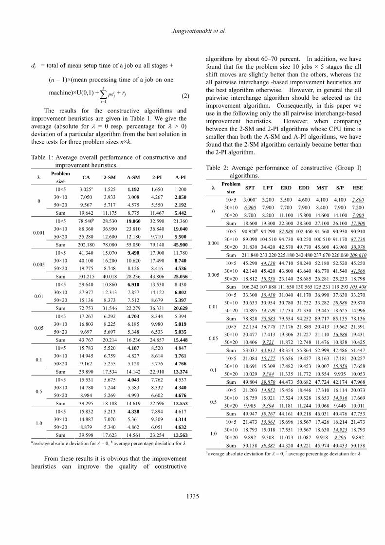
The results for the constructive algorithms and improvement heuristics are given in Table 1. We give the average (absolute for λ = 0 resp. percentage for λ > 0) deviation of a particular algorithm from the best solution in these tests for three problem sizes n×k. Table 1: Average overall performance of constructive and

improvement heuristics.

λ Problem

size CA 2-SM A-SM 2-PI A-PI

10×5 30×10 50×20

3.025a

7.050 9.567

1.525 3.933 5.717

1.192 3.008 4.575

1.650 4.267 5.550

1.200 2.050 2.192

0

Sum 19.642 11.175 8.775 11.467 5.442 10×5

30×10 50×20

78.540b

88.360 35.280

28.530 36.950 12.600

19.060 23.810 12.180

32.590 36.840 9.710

21.360 19.040 5.500

0.001

Sum 202.180 78.080 55.050 79.140 45.900 10×5

30×10 50×20

41.340 40.100 19.775

15.070 16.200 8.748

9.490 10.620 8.126

17.900 17.490 8.416

11.780 8.740 4.536

0.005

Sum 101.215 40.018 28.236 43.806 25.056 10×5

30×10 50×20

29.640 27.977 15.136

10.860 12.313 8.373

6.910 7.857 7.512

13.530 14.122 8.679

8.430 6.802 5.397

0.01

Sum 72.753 31.546 22.279 36.331 20.629 10×5

30×10 50×20

17.267 16.803 9.697

6.292 8.225 5.697

4.703 6.185 5.348

8.344 9.980 6.533

5.394 5.019 5.035

0.05

Sum 43.767 20.214 16.236 24.857 15.448 10×5

30×10 50×20

15.783 14.945 9.162

5.520 6.759 5.255

4.187 4.827 5.128

8.520 8.614 5.776

4.847 3.761 4.766

0.1

Sum 39.890 17.534 14.142 22.910 13.374 10×5

30×10 50×20

15.531 14.780 8.984

5.675 7.244 5.269

4.043 5.583 4.993

7.762 8.332 6.602

4.537 4.340 4.676

0.5

Sum 39.295 18.188 14.619 22.696 13.553 10×5

30×10 50×20

15.832 14.887 8.879

5.213 7.070 5.340

4.338 5.361 4.862

7.894 9.309 6.051

4.617 4.314 4.632

1.0

Sum 39.598 17.623 14.561 23.254 13.563 a average absolute deviation for λ = 0, b average percentage deviation for λ

From these results it is obvious that the improvement

heuristics can improve the quality of constructive

algorithms by about 60–70 percent. In addition, we have found that for the problem size 10 jobs × 5 stages the all shift moves are slightly better than the others, whereas the all pairwise interchange -based improvement heuristics are the best algorithm otherwise. However, in general the all pairwise interchange algorithm should be selected as the improvement algorithm. Consequently, in this paper we use in the following only the all pairwise interchange-based improvement heuristics. However, when comparing between the 2-SM and 2-PI algorithms whose CPU time is smaller than both the A-SM and A-PI algorithms, we have found that the 2-SM algorithm certainly became better than the 2-PI algorithm.

Table 2: Average performance of constructive (Group I)

algorithms.

λ Problem

size SPT LPT ERD EDD MST S/P HSE

10×5 30×10 50×20

3.000a

6.900 8.700

3.200 7.900 8.200

3.500 7.700 11.100

4.600 7.900

15.800

4.100 8.400

14.600

4.100 7.900

14.100

2.800 7.200 7.900

0

Sum 18.600 19.300 22.300 28.300 27.100 26.100 17.90010×5

30×10 50×20

90.920b

89.09031.830

94.290 104.510 34.420

87.880 94.730 42.570

102.460 90.250 49.770

91.560100.51045.600

90.93091.17043.960

90.91087.73030.970

0.001

Sum 211.840 233.220 225.180 242.480 237.670 226.060 209.61010×5

30×10 50×20

45.29042.14018.812

44.130 45.420 18.338

44.710 43.800 23.140

58.240 43.640 28.685

52.18046.77026.281

52.52041.54025.233

45.25041.36018.798

0.005

Sum 106.242 107.888 111.650 130.565 125.231 119.293 105.40810×5

30×10 50×20

33.30030.63314.895

30.430 30.954 14.199

31.040 30.780 17.734

41.170 31.752 21.330

36.99033.28219.445

37.63028.88018.625

33.27029.87014.996

0.01

Sum 78.828 75.583 79.554 94.252 89.717 85.135 78.13610×5

30×10 50×20

22.15420.47710.406

16.778 17.413 9.721

17.176 19.306 11.872

21.889 21.227 12.748

20.41321.11011.476

19.66216.98610.838

21.59119.43110.425

0.05

Sum 53.037 43.912 48.354 55.864 52.999 47.486 51.44710×5

30×10 50×20

21.08418.69110.029

15.177 15.309 9.384

15.656 17.482 11.335

19.457 19.453 11.772

18.16319.00710.554

17.18115.0589.935

20.25717.65810.053

0.1

Sum 49.804 39.870 44.473 50.682 47.724 42.174 47.96810×5

30×10 50×20

21.20318.7599.985

14.852 15.021 9.394

15.456 17.524 11.181

18.446 19.528 11.244

17.31018.65310.068

16.11414.9169.446

20.07317.66910.011

0.5

Sum 49.947 39.267 44.161 49.218 46.031 40.476 47.75310×5

30×10 50×20

21.47318.7939.892

15.061 15.018 9.308

15.696 17.551 11.073

18.567 19.567 11.087

17.42618.6309.918

16.21414.9239.296

21.47318.7939.892

1.0

Sum 50.158 39.387 44.320 49.221 45.974 40.433 50.158a average absolute deviation for λ = 0, b average percentage deviation for λ

1335


Next, we present the constructive algorithms that are separated into four main groups. The first heuristic group includes the simple dispatching rules such as SPT, LPT, ERD, EDD, MST, S/P, and HSE. The second heuristic group includes the flow shop makespan heuristics adapted such as PAL, CDS, GUP, DAN, and NEH. The third and fourth heuristic groups are generated from the first two groups of heuristics where the solutions are improved by the selected polynomial improvement algorithm based on all pairwise interchange-based improvement heuristics, and they are denoted by the first letter “I” in front of the letters describing the heuristics of the first two groups. Table 3: Average performance of constructive (Group II)

algorithms. λ Problem size PAL CDS GUP DAN NEH

10×5 30×10 50×20

2.700a

7.700 9.400

2.200 6.100 6.600

2.800 7.300 8.600

2.600 7.800 8.800

0.700 1.800 1.000

0

Sum 19.800 14.900 18.700 19.200 3.500 10×5 30×10 50×20

73.220b

101.410 37.030

61.630 77.990 27.000

77.800 94.510 34.620

70.370 98.410 35.200

10.470 29.980 10.320

0.001

Sum 211.660 166.620 206.930 203.980 50.770 10×5 30×10 50×20

38.870 44.290 20.046

31.010 34.330 15.791

41.540 42.650 18.867

36.150 43.740 18.902

6.250 11.500 4.411

0.005

Sum 103.206 81.131 103.057 98.792 22.161 10×5 30×10 50×20

28.570 29.870 15.440

22.230 23.506 12.655

30.560 29.744 14.646

25.780 29.561 14.514

4.710 6.887 3.160

0.01

Sum 73.880 58.391 74.950 69.855 14.757 10×5 30×10 50×20

18.069 16.766 10.355

12.421 13.394 8.400

19.019 17.207 9.898

15.633 15.928 9.457

2.399 2.386 0.765

0.05

Sum 45.190 34.215 46.124 41.018 5.550 10×5 30×10 50×20

17.073 14.637 9.877

11.196 11.722 8.016

17.585 15.071 9.523

14.471 13.784 8.985

2.097 1.470 0.479

0.1

Sum 41.587 30.934 42.179 37.240 4.046 10×5 30×10 50×20

17.373 14.368 9.754

11.176 11.768 7.933

17.221 14.794 9.489

14.448 13.488 8.866

2.700 0.869 0.436

0.5

Sum 41.495 30.877 41.504 36.802 4.005 10×5 30×10 50×20

17.674 14.367 9.651

11.400 11.785 7.837

17.418 14.780 9.399

14.701 13.477 8.766

2.885 0.964 0.428

1.0


The results for the constructive and polynomial

improvement algorithms are given in Table 2 through Table

5. From these results it can be seen that the improvement algorithms in the fourth heuristic group improved from flow shop makespan heuristics from the second heuristic group (i.e., PAL, CDS, GUP, DAN, and NEH) are better than the dispatching rules in the first heuristic group (i.e., SPT, LPT, ERD, EDD, MST, S/P, and HSE) as well as the third heuristic group improved from them. Table 4: Average performance of improvement (Group III)

algorithms. λ Problem size ISPT ILPT IERD IEDD IMST IS/P IHSE

10×5 30×10 50×20

1.400a

2.1001.300

1.300 2.500 2.300

1.200 2.400 3.000

1.000 1.500 3.000

1.3001.2004.900

1.3001.8003.300

1.1002.1001.700

0

Sum 4.800 6.100 6.600 5.500 7.400 6.400 4.90010×5

30×10 50×20

16.220b

20.3106.730

24.020 18.910 5.150

12.550 18.970 7.690

13.710 13.200 5.010

18.94015.7104.040

18.87013.9106.960

23.88019.0902.990

0.001

Sum 43.260 48.080 39.210 31.920 38.690 39.740 45.96010×5

30×10 50×20

10.0009.6903.924

13.410 8.150 5.228

8.170 8.610 5.514

8.650 7.530 6.051

11.9907.5203.554

11.7406.6105.631

14.84010.3003.922

0.005

Sum 23.614 26.788 22.294 22.231 23.064 23.981 29.06210×5

30×10 50×20

8.8906.3734.699

9.450 9.709 6.427

7.030 5.676 5.749

6.640 6.753 6.264

7.6904.7626.890

9.5404.0766.583

9.0809.0965.198

0.01

Sum 19.962 25.586 18.455 19.657 19.342 20.199 23.37410×5

30×10 50×20

5.4764.8204.778

5.281 6.313 5.247

4.900 2.768 5.438

6.629 6.397 7.221

5.6435.4316.010

5.6204.8936.711

7.1946.4315.028

0.05

Sum 15.074 16.841 13.106 20.247 17.084 17.224 18.65310×5

30×10 50×20

4.5463.2555.169

5.404 4.743 4.241

4.787 1.718 5.024

6.318 5.523 6.681

5.7214.9575.831

4.8775.0335.788

5.7634.6195.173

0.1

Sum 12.970 14.388 11.529 18.522 16.509 15.698 15.55510×5

30×10 50×20

4.9693.9295.453

4.932 5.283 4.244

5.195 2.404 5.090

5.707 6.727 6.215

6.2875.1355.900

4.6296.8974.725

5.4144.7305.406

0.5

Sum 14.351 14.459 12.689 18.649 17.322 16.251 15.55010×5

30×10 50×20

5.0184.1555.346

5.073 4.838 4.147

5.268 2.421 5.107

5.741 6.843 6.079

5.9355.9325.731

4.8406.9404.523

5.0184.1555.346

1.0


Among the simple dispatching rules (heuristic Group

I), the SPT, LPT, ERD, and HSE rules are good dispatching rules. However, in general the HSE rule outperforms the other dispatching rules for λ < 0.01, and the LPT rule is better than the other rules otherwise. Among the adapted flow shop makespan heuristics in heuristic Group II, the NEH algorithm is clearly the best algorithm among all

1336


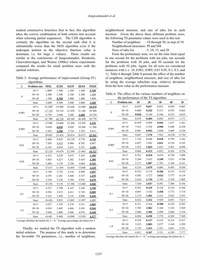
studied constructive heuristics (but in fact, this algorithm takes the convex combination of both criteria into account when selecting partial sequences). The CDS algorithm is certainly the algorithm on the second rank (but it is substantially worse than the NEH algorithm even if the makespan portion in the objective function value is dominant, i.e. for large λ values). These results are similar to the conclusions of Jungwattanakit, Reodecha, Chaovalitwongse, and Werner (2006c) whose experiments compared the results for small problem sizes with the optimal solutions.

Table 5: Average performance of improvement (Group IV)

algorithms. λ Problem size IPAL ICDS IGUP IDAN INEH

10×5 30×10 50×20

1.400a

2.500 1.700

1.300 2.300 0.700

1.100 2.100 2.000

1.300 2.300 1.400

0.700 1.800 1.000

0

Sum 5.600 4.300 5.200 5.000 3.500 10×5 30×10 50×20

35.200b

17.750 8.750

23.980 18.110 2.640

35.630 21.450 3.260

22.840 21.140 2.460

10.470 29.980 10.320

0.001

Sum 61.700 44.730 60.340 46.440 50.770 10×5 30×10 50×20

13.980 9.650 5.453

14.060 6.050 3.306

15.260 9.020 3.734

12.970 10.200 3.703

6.250 11.500 4.411

0.005

Sum 29.083 23.416 28.014 26.873 22.161 10×5 30×10 50×20

8.460 7.585 6.183

9.810 4.935 4.934

10.130 8.988 3.431

9.770 6.782 5.251

4.710 6.887 3.160

0.01

Sum 22.228 19.679 22.549 21.803 14.757 10×5 30×10 50×20

6.322 5.865 5.486

4.229 4.227 3.139

5.675 5.282 5.538

5.365 5.419 5.064

2.399 2.386 0.765

0.05

Sum 17.673 11.595 16.495 15.848 5.550 10×5 30×10 50×20

5.749 4.193 5.336

3.752 2.241 3.126

4.154 3.848 5.394

4.996 3.537 4.955

2.097 1.470 0.479

0.1

Sum 15.278 9.119 13.396 13.488 4.046 10×5 30×10 50×20

4.327 4.936 5.163

2.790 2.812 3.450

4.147 4.611 5.125

3.346 3.745 4.906

2.700 0.869 0.436

0.5

Sum 14.426 9.052 13.883 11.997 4.005 10×5 30×10 50×20

4.527 4.910 5.044

3.195 2.405 3.808

4.378 4.666 5.046

3.531 3.543 4.976

2.885 0.964 0.428

1.0


Thirdly, we studied the TS algorithm with a random

initial solution. The purpose of this study is to determine the favorable TS parameters, i.e., number of neighbors,

neighborhood structure, and size of tabu list in each iteration. Given the above three different problem sizes, the following TS parameter values were used in this test.

Number of neighbors : 10 through 50, in step of 10 Neighborhood structures : PI and SM Sizes of tabu list : 5, 10, 15, and 20 From the preliminary tests, we set the time limit equal

to one second for the problems with ten jobs, ten seconds for the problems with 30 jobs, and 30 seconds for the problems with 50 jobs. Again, for all tests we considered instances with λ ∈ {0, 0.001, 0.005, 0.01 0.05, 0.1, 0.5, and 1}. Table 6 through Table 8 present the effect of the number of neighbors, neighborhood structure, and size of tabu list by using the average (absolute resp. relative) deviation from the best value as the performance measure.

Table 6: The effect of the various numbers of neighbors on

the performance of the TS algorithm. λ Problem size 10 20 30 40 50

10×5 30×10 50×20

0.029a

0.400

0.050

0.017

0.242

0.146

0.033

0.313

0.346

0.050

0.392

0.533

0.083

0.463

0.625 0

Sum 0.479 0.404 0.692 0.975 1.171 10×5 30×10 50×20

0.954b

7.912

0.981

0.989

5.236

0.945

0.943

4.940

2.040

1.477

5.640

3.409

3.281

6.250

4.250 0.001

Sum 9.847 7.170 7.923 10.526 13.781 10×5 30×10 50×20

1.136

6.057

1.875

0.648

3.942

1.663

0.618

3.611

2.623

0.799

4.134

3.493

1.282

4.195

4.099 0.005

Sum 9.068 6.253 6.852 8.426 9.576 10×5 30×10 50×20

0.781

5.264

2.171

0.419

3.653

1.807

0.474

3.549

2.783

0.730

3.931

3.744

1.099

4.390

4.161 0.01

Sum 8.216 5.879 6.806 8.405 9.650 10×5 30×10 50×20

0.535

4.585

2.410

0.176

3.727

1.734

0.166

3.632

2.793

0.191

3.777

3.338

0.332

4.119

3.905 0.05

Sum 7.530 5.637 6.591 7.306 8.356 10×5 30×10 50×20

0.381

4.067

2.174

0.119

3.542

1.491

0.158

3.458

2.313

0.154

3.773

2.925

0.344

3.714

3.555 0.1

Sum 6.622 5.152 5.929 6.851 7.613 10×5 30×10 50×20

0.331

3.705

2.008

0.164

2.962

1.304

0.108

3.168

2.098

0.228

3.182

2.860

0.282

3.569

3.510 0.5

Sum 6.044 4.430 5.374 6.269 7.360 10×5 30×10 50×20

0.358

3.523

2.129

0.127

2.805

1.415

0.152

2.877

2.321

0.218

3.169

2.861

0.327

3.299

3.551 1.0


1337


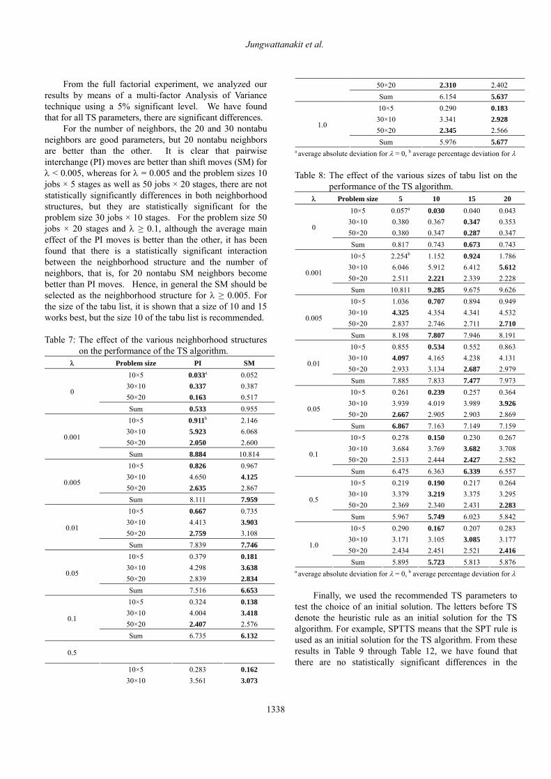
From the full factorial experiment, we analyzed our results by means of a multi-factor Analysis of Variance technique using a 5% significant level. We have found that for all TS parameters, there are significant differences.

For the number of neighbors, the 20 and 30 nontabu neighbors are good parameters, but 20 nontabu neighbors are better than the other. It is clear that pairwise interchange (PI) moves are better than shift moves (SM) for λ < 0.005, whereas for λ = 0.005 and the problem sizes 10 jobs × 5 stages as well as 50 jobs × 20 stages, there are not statistically significantly differences in both neighborhood structures, but they are statistically significant for the problem size 30 jobs × 10 stages. For the problem size 50 jobs × 20 stages and λ ≥ 0.1, although the average main effect of the PI moves is better than the other, it has been found that there is a statistically significant interaction between the neighborhood structure and the number of neighbors, that is, for 20 nontabu SM neighbors become better than PI moves. Hence, in general the SM should be selected as the neighborhood structure for λ ≥ 0.005. For the size of the tabu list, it is shown that a size of 10 and 15 works best, but the size 10 of the tabu list is recommended.

Table 7: The effect of the various neighborhood structures

on the performance of the TS algorithm. λ Problem size PI SM

10×5 30×10 50×20

0.033a

0.337 0.163

0.052 0.387 0.517

0

Sum 0.533 0.955 10×5 30×10 50×20

0.911b

5.923 2.050

2.146 6.068 2.600

0.001

Sum 8.884 10.814 10×5 30×10 50×20

0.826 4.650 2.635

0.967 4.125 2.867

0.005

Sum 8.111 7.959 10×5 30×10 50×20

0.667 4.413 2.759

0.735 3.903 3.108

0.01

Sum 7.839 7.746 10×5 30×10 50×20

0.379 4.298 2.839

0.181 3.638 2.834

0.05

Sum 7.516 6.653 10×5 30×10 50×20

0.324 4.004 2.407

0.138 3.418 2.576

0.1

Sum 6.735 6.132

0.5

10×5 30×10

0.283 3.561

0.162 3.073

50×20 2.310 2.402 Sum 6.154 5.637 10×5 30×10 50×20

0.290 3.341 2.345

0.183 2.928 2.566

1.0

Sum 5.976 5.677 a average absolute deviation for λ = 0, b average percentage deviation for λ Table 8: The effect of the various sizes of tabu list on the

performance of the TS algorithm. λ Problem size 5 10 15 20

10×5 30×10 50×20

0.057a

0.380

0.380

0.030

0.367

0.347

0.040

0.347

0.287

0.043

0.353

0.347 0

Sum 0.817 0.743 0.673 0.743 10×5

30×10 50×20

2.254b

6.046

2.511

1.152

5.912

2.221

0.924

6.412

2.339

1.786

5.612

2.228 0.001

Sum 10.811 9.285 9.675 9.626 10×5

30×10 50×20

1.036

4.325

2.837

0.707

4.354

2.746

0.894

4.341

2.711

0.949

4.532

2.710 0.005

Sum 8.198 7.807 7.946 8.191 10×5

30×10 50×20

0.855

4.097

2.933

0.534

4.165

3.134

0.552

4.238

2.687

0.863

4.131

2.979 0.01

Sum 7.885 7.833 7.477 7.973 10×5

30×10 50×20

0.261

3.939

2.667

0.239

4.019

2.905

0.257

3.989

2.903

0.364

3.926

2.869 0.05

Sum 6.867 7.163 7.149 7.159 10×5

30×10 50×20

0.278

3.684

2.513

0.150

3.769

2.444

0.230

3.682

2.427

0.267

3.708

2.582 0.1

Sum 6.475 6.363 6.339 6.557 10×5

30×10 50×20

0.219

3.379

2.369

0.190

3.219

2.340

0.217

3.375

2.431

0.264

3.295

2.283 0.5

Sum 5.967 5.749 6.023 5.842 10×5

30×10 50×20

0.290

3.171

2.434

0.167

3.105

2.451

0.207

3.085

2.521

0.283

3.177

2.416 1.0

Sum 5.895 5.723 5.813 5.876 a average absolute deviation for λ = 0, b average percentage deviation for λ

Finally, we used the recommended TS parameters to

test the choice of an initial solution. The letters before TS denote the heuristic rule as an initial solution for the TS algorithm. For example, SPTTS means that the SPT rule is used as an initial solution for the TS algorithm. From these results in Table 9 through Table 12, we have found that there are no statistically significant differences in the

1338


different initial solutions for the problem sizes 10 jobs × 5 stages and 30 jobs × 10 stages, but it became statistically significantly different in the problem size 50 jobs × 20 stages especially for λ ≥ 0.05 we have found that algorithms INEHTS and NEHTS are better than the others. Consequently, in general algorithms INEHTS and NEHTS are good choices for the TS algorithm with using a biased initial solution. Table 9: Comparison of the TS algorithm with different

initial solutions (Group I).

λ Problem

size SPTTS LPTTS ERDTS EDDTS MSTTS S/PTS HSETS

10×5 30×10 50×20

0.020a

0.220

0.060

0.000

0.220

0.060

0.0200.2600.100

0.000

0.240

0.060

0.020

0.260

0.040

0.0000.2400.060

0.0400.2200.020

0

Sum 0.300 0.280 0.380 0.300 0.320 0.300 0.280 10×5

30×10 50×20

0.014b

3.674

0.667

0.090

4.649

0.938

0.0714.3771.415

0.589

4.152

0.937

0.023

4.544

0.634

0.0644.9280.614

1.0273.9540.512

0.001

Sum 4.355 5.677 5.863 5.678 5.201 5.606 5.493 10×5

30×10 50×20

0.306

2.892

1.363

0.984

3.177

1.223

0.9122.8471.491

0.280

3.034

1.285

1.067

3.484

0.838

0.7702.7351.044

0.4213.1070.992

0.005

Sum 4.561 5.384 5.250 4.599 5.389 4.549 4.520 10×5

30×10 50×20

0.598

3.063

1.068

0.551

3.562

0.851

0.3562.3731.180

0.206

3.003

1.451

0.377

3.189

0.690

0.3732.5770.944

0.3233.2371.113

0.01

Sum 4.729 4.964 3.909 4.660 4.256 3.894 4.673 10×5

30×10 50×20

0.039

3.252

1.064

0.033

3.513

0.959

0.0292.3571.146

0.049

3.499

1.031

0.059

2.677

0.764

0.0263.1171.040

0.0953.3881.206

0.05

Sum 4.355 4.505 3.532 4.579 3.500 4.183 4.689 10×5

30×10 50×20

0.039

2.698

0.947

0.057

2.633

1.183

0.0091.9471.166

0.021

2.440

1.470

0.030

2.231

0.956

0.0082.4770.991

0.0202.7691.262

0.1

Sum 3.685 3.872 3.122 3.931 3.218 3.476 4.052 10×5

30×10 50×20

0.061

2.307

0.938

0.015

2.396

1.047

0.0551.8721.228

0.039

2.421

1.336

0.031

2.152

1.027

0.0192.4710.936

0.1072.1801.041

0.5

Sum 3.306 3.458 3.155 3.796 3.210 3.426 3.327 10×5

30×10 50×20

0.096

2.264

0.878

0.059

2.517

0.981

0.0541.8081.107

0.067

2.342

1.300

0.011

2.560

0.931

0.0481.9250.986

0.0962.2660.878

1.0

Sum 3.237 3.557 2.969 3.709 3.502 2.960 3.239 a average absolute deviation for λ = 0, b average percentage deviation for λ

6. CONCLUSIONS

In this paper, some constructive algorithms have first

been investigated for minimizing a convex combination of

makespan and the number of tardy jobs for the hybrid flow shop problem with unrelated parallel machines and setup times, which is often occurring in the real world problems. All algorithms are based on the list scheduling principle by developing job sequences for the first stage and assigning and sequencing the remaining stages by both the permutation and FIFO approaches.

Table 10: Comparison of the TS algorithm with different

initial solutions (Group II). λ Problem size PALTS CDSTS GUPTS DANTS NEHTS

10×5 30×10 50×20

0.000 0.260 0.120

0.000 0.340 0.020

0.020 0.220 0.060

0.020 0.280 0.040

0.000 0.180 0.000

0

Sum 0.380 0.360 0.300 0.340 0.180 10×5 30×10 50×20

0.163 4.142 0.648

0.100 3.715 0.544

1.041 4.193 0.761

1.528 4.993 0.470

0.166 3.413 0.343

0.001

Sum 4.953 4.359 5.995 6.991 3.922 10×5 30×10 50×20

0.615 2.776 1.395

1.179 2.967 0.876

0.602 3.014 0.985

0.649 3.069 1.238

1.076 3.353 0.540

0.005

Sum 4.786 5.022 4.601 4.956 4.969 10×5 30×10 50×20

0.420 3.490 0.970

0.779 2.851 1.371

0.394 3.538 1.107

0.398 3.108 1.384

0.664 3.068 0.539

0.01

Sum 4.880 5.001 5.039 4.890 4.271 10×5 30×10 50×20

0.039 3.036 1.083

0.029 3.030 1.421

0.022 3.032 1.303

0.058 3.255 1.356

0.042 2.128 0.491

0.05

Sum 4.158 4.480 4.357 4.670 2.661 10×5 30×10 50×20

0.017 2.515 0.822

0.025 2.295 1.182

0.014 2.161 1.064

0.033 1.978 1.327

0.030 1.839 0.415

0.1

Sum 3.354 3.502 3.239 3.338 2.285 10×5 30×10 50×20

0.006 2.549 0.904

0.039 2.426 1.306

0.015 1.801 0.798

0.049 2.341 1.132

0.039 1.407 0.327

0.5

Sum 3.458 3.771 2.615 3.522 1.773 10×5 30×10 50×20

0.042 2.787 1.172

0.069 2.468 1.356

0.029 2.243 1.041

0.075 2.449 1.289

0.047 1.741 0.362

1.0


The constructive algorithms are compared to the best

solutions. It is shown that in particular, for the simple dispatching rules the SPT, LPT, ERD, and HSE rules are good algorithms whereas for the flow shop makespan heuristics, the NEH algorithm is most superior to the other constructive algorithms. When we have applied the polynomial improvement algorithm, we have found that the

1339


all-pairwise interchange algorithm is a good improvement algorithm. Next, we used TS-based algorithms as improving algorithms. Before we studied the influence of the initial solution on the performance of the TS algorithm, we tested the TS parameters, i.e., number of neighbors, neighborhood structure, and size of tabu list. We have found that a constant number of 20 neighbors works best. The neighborhood structures should be based on shift moves for λ ≥ 0.05 and on pairwise interchanges of jobs otherwise. The size of tabu list should be selected as 10. For the recommended TS parameters, we investigated the selection of a starting solution by using several constructive and improvement algorithms. The variants INEHTS and NEHTS can both be recommended in general.


initial solutions (Group III).

λ Problem

size ISPTT

S ILPTT

S IERDT

S IEDDT

S IMSTT

S IS/PTS

IHSETS

10×5 30×10 50×20

0.000a

0.280

0.100

0.000

0.220

0.120

0.000

0.220

0.080

0.020

0.260

0.000

0.000

0.240

0.000

0.0000.2400.040

0.0000.2200.000

0

Sum 0.380 0.340 0.300 0.280 0.240 0.280 0.22010×5

30×10 50×20

0.531b

4.107

0.847

0.575

3.829

1.014

0.044

4.898

0.797

0.544

3.386

1.174

0.525

2.985

0.555

0.5263.9630.805

0.0433.7430.358

0.001

Sum 5.485 5.418 5.739 5.104 4.065 5.294 4.14410×5

30×10 50×20

0.573

2.906

0.932

1.279

3.068

1.745

1.044

3.140

2.025

0.589

2.514

2.273

0.272

2.904

0.803

0.4133.5091.730

0.7953.1371.122

0.005

Sum 4.411 6.092 6.209 5.376 3.979 5.652 5.05410×5

30×10 50×20

0.468

3.824

1.241

0.481

3.346

1.775

0.477

2.963

1.635

0.485

2.936

1.437

0.405

3.065

1.266

0.3442.9681.132

0.3123.4971.470

0.01

Sum 5.533 5.602 5.075 4.858 4.736 4.444 5.27910×5

30×10 50×20

0.076

3.094

1.027

0.052

2.692

1.146

0.057

2.743

1.700

0.052

3.343

1.494

0.065

2.860

1.056

0.0412.6971.316

0.0392.5881.152

0.05

Sum 4.196 3.891 4.500 4.889 3.981 4.054 3.77910×5

30×10 50×20

0.010

2.569

0.946

0.035

2.628

1.304

0.031

2.107

1.302

0.046

2.528

1.222

0.039

2.259

1.052

0.0552.1661.071

0.0102.6611.229

0.1

Sum 3.524 3.966 3.440 3.796 3.350 3.292 3.89910×5

30×10 50×20

0.027

2.179

0.927

0.035

2.256

1.249

0.061

2.004

1.172

0.043

2.276

1.326

0.043

2.127

1.214

0.0312.3211.185

0.0042.1881.061

0.5

Sum 3.133 3.540 3.237 3.645 3.384 3.537 3.25310×5

30×10 50×20

0.037

2.366

0.972

0.065

2.433

1.226

0.066

2.082

1.172

0.035

2.177

1.192

0.075

1.960

1.208

0.0352.1161.060

0.0482.2030.972

1.0


Further research can be done to use other improving algorithms such as genetic or ant colony algorithms. The choice of good parameters for them should be tested. The influence of the starting solution should be investigated. Moreover, hybrid algorithms should be developed by using a tabu search algorithm as a local search algorithm within a genetic algorithm or the other algorithms.


initial solutions (Group IV). λ Problem size IPALTS ICDSTS IGUPTS IDANTS INEHTS

10×5 30×10 50×20

0.000a

0.220

0.140

0.020

0.300

0.040

0.000

0.260

0.060

0.020

0.200

0.040

0.000

0.160

0.000 0

Sum 0.360 0.360 0.320 0.260 0.160 10×5 30×10 50×20

1.024b

4.915

1.087

1.056

4.934

0.380

0.544

4.743

0.369

0.100

4.804

0.758

0.534

3.421

0.350 0.001

Sum 7.026 6.370 5.656 5.662 4.305 10×5 30×10 50×20

0.832

3.182

2.089

1.103

3.329

0.676

0.527

2.910

0.778

0.732

3.278

1.441

0.721

3.461

0.543 0.005

Sum 6.103 5.108 4.215 5.451 4.725 10×5 30×10 50×20

0.628

3.274

1.782

0.387

3.109

1.124

0.286

3.316

0.942

0.603

3.597

1.557

0.706

2.994

0.539 0.01

Sum 5.684 4.620 4.544 5.757 4.239 10×5 30×10 50×20

0.059

3.512

1.531

0.054

3.238

0.891

0.070

2.731

1.189

0.022

2.439

1.302

0.029

2.233

0.491 0.05

Sum 5.101 4.183 3.990 3.763 2.753 10×5 30×10 50×20

0.009

2.682

1.266

0.021

2.356

1.036

0.012

2.620

0.782

0.010

1.914

1.284

0.012

1.832

0.416 0.1

Sum 3.957 3.413 3.414 3.208 2.260 10×5 30×10 50×20

0.019

1.999

1.495

0.041

2.288

0.876

0.044

2.121

1.056

0.044

2.049

0.937

0.039

1.456

0.314 0.5

Sum 3.514 3.205 3.221 3.030 1.809 10×5 30×10 50×20

0.016

2.654

1.328

0.024

2.181

1.033

0.047

2.179

1.020

0.011

2.053

1.358

0.035

1.747

0.362 1.0


ACKNOWLEDGMENT This work was supported by Department of Industrial

Engineering, Chulalongkorn University. The fourth author has been supported by INTAS

(project 03-51-5501).

1340


REFERENCES

Alisantoso, D., Khoo, L.P., and Jiang, P.Y. (2003) An

immune algorithm approach to the scheduling of a flexible PCB flow shop, The International Journal of Advanced Manufacturing Technology, 22(11), 819-827.

Blum, C., and Roli, A. (2003) Metaheuristics in combinatorial optimization: Overview and conceptual comparison, ACM Computing Surveys, 35(3), 268–308.

Campbell, H.G., Dudek, R.A., and Smith, M.L. (1970) A Heuristic algorithm for the n-Job m-Machine sequencing problem, Management Science, 16(10), 630–637.

Dannenbring, D.G. (1977) An evaluation of flow shop sequencing heuristics, Management Science, 23(11),1174-1182.

Garey, M.R., and Johnson, D.S. (1979) Computers and Intractability: A Guide to the Theory of NP-Completeness, CA: Freeman, San Francisco.

Glover, F., and Laguna, M. (1993) Tabu search. In C.R.Reeves (ed), Modern Heuristic Techniques for Combinatorial Problems (UK: Blackwell Scientific Publications), Oxford, chapter 3, 70-150.

Glover, F. (1986) Future paths for integer programming and links to artificial intelligence, Computers and Operations Research, 13(5), 533–549.

Gupta, J.N.D (1971) A functional heuristic algorithm for the flow-shop scheduling problem, Operations Research Quarterly, 22(1), pp. 39-47.

Gupta, J.N.D., Krüger, K., Lauff, V., Werner, F., and Sotskov, Y.N. (2002) Heuristics for hybrid flow shops with controllable processing times and assignable due dates, Computers & Operations Research, 29(10), 1417-1439.

Jungwattanakit, J., Reodecha, M., Chaovalitwongse, P., and Werner, F. (2006a) Solving the hybrid flowshop scheduling problem with unrelated parallel machines and sequence-dependent setup times by simulated annealing algorithm, Proceedings of the 1st International Conference & 7th AUN/SEED-Net Fieldwise Seminar on Manufacturing and Material Process, Kuala Lumpur, Malaysia, 640–645.

Jungwattanakit, J., Reodecha, M., Chaovalitwongse, P., and Werner, F. (2006b) Constructive and simulated annealing heuristics for hybrid flow shops with unrelated parallel machines, Proceedings of the 3rd OR-CRN Operations Research conference 2006, Bangkok, Thailand, 110–121.

Jungwattanakit, J., Reodecha, M., Chaovalitwongse, P., and Werner, F. (2006c) Sequencing heuristics for flexible flow shop scheduling problems with unrelated parallel machines and setup time, Proceedings of the 2006 IE Network National Conference. Bangkok, Thailand. (to appear)

Lin, Hung-Tso., and Liao, Ching-Jong (2003) A case study in a two-stage hybrid flow shop with setup time and dedicated machines, International Journal of Production Economics, 86(2), 133-143.

Nawaz, M., Enscore, Jr. E., Ham, I. (1983) A heuristic algorithm for the m-machine, n-job flowshop sequencing problem, Omega International Journal of Management Science, 11(1), 91–95.

Palmer, D.S. (1965) sequencing jobs through a multi-stage process in the minimum total time--a quick method of obtaining a near optimum, Operations Research Quarterly, 16(1),101–107.

Pinedo, M., and Chao, X. (1999) Operations scheduling with applications in manufacturing and services, Irwin/McGraw-Hill, New York.

Rajendran, C., and Ziegler, H. (2003) Scheduling to minimize the sum of weighted flowtime and weighted tardiness of jobs in a flowshop with sequence-dependent setup times, European Journal of Operational Research, 149(3), 513–522.

Wang, W. (2005) Flexible Flow Shop Scheduling: Optimum, heuristics, and artificial intelligence solution, Expert Systems, 22(2), 78 – 85.

Wang, W., and Hunsucker, J.L. (2003) An evaluation of the CDS heuristic in flow shops with multiple processors, Journal of the Chinese Institute of Industrial Engineers, 20 (3), 295-304. AUTHOR BIOGRAPHIES Jitti Jungwattanakit is a Ph.D. student in Industrial Engineering Department, Chulalongkorn University, Thailand. His main research areas are Scheduling, Operations Research, and Simulation. His email address is <[email protected]>. Manop Reodecha is an Assistant Professor in Industrial Engineering Department, Chulalongkorn University, Thailand. He received a Ph.D. in Industrial Engineering from North Carolina State University. His main research areas are Logistics and Supply Chain Management, Production and Operations Management, and Information Systems. His email address is <[email protected]>.

Paveena Chaovalitwongse is an Assistant Professor in Industrial Engineering Department, Chulalongkorn University, Thailand. She received a Ph.D. degree from University of Florida. Her main research areas are Operations Research, Supply Chain and Logistics Management, and Production Planning and Control. Her email address is <[email protected]>.

1341


Frank Werner is an Extraordinary Professor at the Faculty of Mathematics of the Otto-von-Guericke-University, Germany. He received a Ph.D. degree from the TU Magdeburg. His main research areas are Scheduling,

Stability investigations, Graph coloring problems, Logistics, and Supply Chains. His email address is <[email protected]>.

1342

sequencing and tabu search heuristics for hybrid flow ...werner/t3d1.pdf · sequencing and tabu...

Documents