sensitivity of gnss radio occultation data to horizontal ...wegc · sensitivity of gnss radio...

Physics and Chemistry of the Earth 29 (2004) 225–240

www.elsevier.com/locate/pce

Sensitivity of GNSS radio occultation data to horizontalvariability in the troposphere

Ulrich Foelsche *, Gottfried Kirchengast

Institute for Geophysics, Astrophysics, and Meteorology (IGAM), University of Graz, Universit€atsplatz 5, A-8010 Graz, Austria

Abstract

We addressed the sensitivity of Global Navigation Satellite System (GNSS) radio occultation (RO) measurements to atmospheric

horizontal variability based on realistically simulated data. Retrieved parameters from refractivity via pressure, and geopotential

height to dry temperature were investigated. The errors in a realistic horizontally variable atmosphere relative to errors in a

spherically symmetric atmosphere were quantified based on an ensemble of 60 occultation events. These events have been simulated

using ray tracing through a representative European Centre for Medium-Range Weather Forecasts (ECMWF) T213L50 analysis

field with and without horizontal variability, respectively. Below �7 km height biases and standard deviations of all parameters

under spherical symmetry are significantly smaller than corresponding errors in a realistic atmosphere with horizontal variability.

The relevance of the geometry of reference profiles was assessed in this context as well. A significant part of the total error below �7

km can be attributed to adopting reference profiles vertically at mean tangent point locations instead of extracting them along actual

3D tangent point trajectories. The sensitivity of retrieval products to the angle-of-incidence of occultation rays relative to the

boresight direction of the receiving antenna was analyzed for three different azimuth sectors (0–10�, 20–30�, 40–50�) with 20 events

in each sector. Below about 7 km, most errors were found to increase with increasing angle of incidence. Dry temperature biases

between 7 and 20 km exhibit no relevant increase with increasing angle of incidence, which is favorable regarding the climate

monitoring utility of the data.

� 2004 Elsevier Ltd. All rights reserved.

Keywords: Remote sensing; Atmospheric propagation; Inverse theory; Pressure, density, and temperature

1. Introduction

A detailed description of the Global Navigation Sa-

tellite System (GNSS) radio occultation (RO) technique

and estimates of errors in the troposphere caused by

horizontal variation can be found in Kursinski et al.

(1997). Ahmad and Tyler (1999) performed an analytical

approach to the errors introduced by refractivity gra-

dients. The simulation study by Healy (2001) focused on

bending angle and impact parameter errors caused byhorizontal refractivity gradients in the troposphere.

1.1. Study objectives

We investigated the sensitivity of atmospheric profiles

retrieved from Global Navigation Satellite System

*Corresponding author. Tel.: +43-316-380-8590; fax: +43-316-380-

9825.

E-mail address: [email protected] (U. Foelsche).

1474-7065/$ - see front matter � 2004 Elsevier Ltd. All rights reserved.

doi:10.1016/j.pce.2004.01.007

(GNSS) RO data to atmospheric horizontal variability

in a twofold manner: first, the errors in a (realistic)horizontally variable atmosphere are compared with

errors in a spherically symmetric atmosphere, based on

an ensemble of 60 occultation events (using an Euro-

pean Centre for Medium-Range Weather Forecasts,

ECMWF, T213L50 analysis field with and without

horizontal variability). The difference incurred by either

assuming the ‘‘true’’ profile vertically at a mean event

location (the common practice) or more precisely alongthe estimated 3D tangent point trajectory traced out

during the event was assessed in this context as well.

Second, the sensitivity of retrieval products to the angle-

of-incidence of occultation rays relative to the boresight

direction of the receiving antenna (aligned with the LEO

orbit plane) was analyzed based on ensembles of events

(from the same ECMWF analysis field) for three dif-

ferent angle-of-incidence classes (±10�, ±20� to ±30�,±40� to ±50�). This provided important insights into

how much the climate monitoring utility of GNSS

occultation data depends on occultation event geometry.

mail to: [email protected]

226 U. Foelsche, G. Kirchengast / Physics and Chemistry of the Earth 29 (2004) 225–240

1.2. Study overview

The EGOPS software tool (End-to-end GNSS

Occultation Performance Simulator, version 4.0) was

used to generate realistically simulated measurements of

the observables refractivity, total atmospheric pressure,

geopotential height, and (dry) temperature. For a de-tailed description of EGOPS (see Kirchengast, 1998;

Kirchengast et al., 2001). Section 2 gives an overview

on the experimental setup. Results on the sensitivity

to horizontal variability are presented in Section 3, the

results on sensitivity to angle-of-incidence are shown

and discussed in Section 4. Conclusions and an outlook

are finally provided in Section 5.

2. Experimental setup

2.1. Geometry

We assumed a full constellation of 24 Global Posi-

tioning System (GPS) satellites as transmitters and a

GNSS Receiver for Atmospheric Sounding (GRAS)sensor onboard the METOP satellite (nominal orbit

altitude �830 km). With such a constellation a total of

Fig. 1. Schematic illustration of azimuth sectors used in the study:

sector 1 (dark gray), sector 2 (medium gray), and sector 3 (light gray).

Rising events are observed with the antenna oriented in flight direction

(0� azimuth), setting events with the aft-looking antenna.

Table 1

Azimuth sectors used in this study

Sector 1 Sector 2

Rising events 0� to )10� )20� to )30�0� to +10� +20� to +30�

Setting events 170� to 180� 150� to 160�180� to 190� 200� to 210�

No. of events 20 20

We selected 5 rising or 5 setting events, respectively, in each of the 12 sub-s

somewhat over 500 rising and setting occultation events

per day can be obtained during a simulation over a 24 h

period. The simulated day was September 15, 1999, the

date of the ECMWF analysis field used in the forward

modeling.

We collected occultation events in three different

azimuth sectors relative to the boresight direction ofthe receiving antennae. A schematic illustration of this

division into several ‘‘angle-of-incidence’’ sectors is

given in Fig. 1, while Table 1 summarizes the simula-

tion design in terms of numbers of events simulated per

sub-sector defined. Sector 1 (dark gray in Fig. 1) com-

prises azimuth angles between )10� and +10� (rising

occultations) plus angles between 170� and 190� (sett-

ing occultations). Angles of incidence in the range ofj25�j � 5�, symmetric to the orbit plane, compose Sector

2 (four medium gray sub-sectors in Fig. 1). Sector 3

corresponds to angles of incidence in the range of

j45�j � 5�, symmetric to the orbit plane (light gray in

Fig. 1).

With restriction to the described azimuth sectors we

obtained a total of 321 occultation events during the

selected 24 h period. The geographic distribution isshown in the top panel of Fig. 2. From this sample of

321 occultations we selected 20 events per azimuth sec-

tor (60 events in total) in order to keep computational

expenses limited. Selection criteria were:

• Uniform distribution in latitude an longitude in each

sector.

• Equal density over oceans and over continents ineach sector.

• Same amount of rising and setting occultations (see

Table 1).

The geographic distribution of the 60 selected occul-

tation events is displayed in the bottom panel of Fig. 2.

It is visible that a reasonably representative coverage is

achieved with the selected ensemble.

2.2. Forward modeling

High resolution (T213L50) analysis fields from the

European Centre for Medium-Range Weather Forecasts

(ECMWF) for September 15, 1999, 12 UT, were used to

Sector 3 No. of events

)40� to )50� 15

+40� to 50� 15

130� to 140� 15

220� to 230� 15

20 60

ectors, leading to a total ensemble of 60 events.

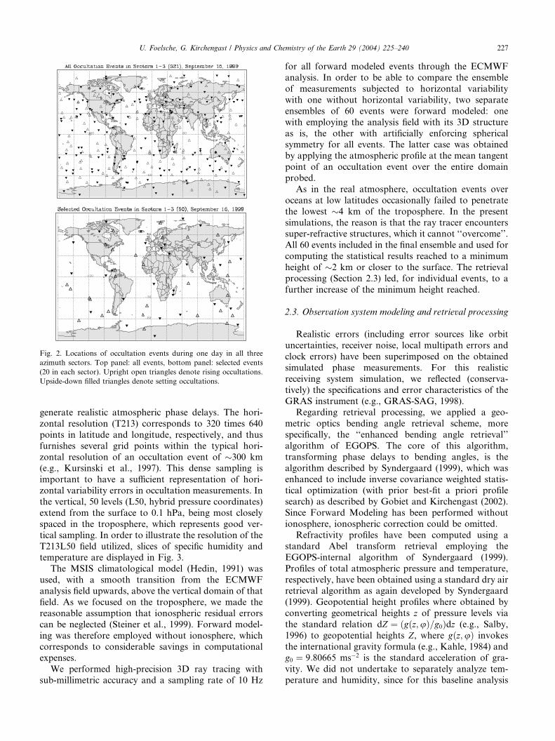
Fig. 2. Locations of occultation events during one day in all three

azimuth sectors. Top panel: all events, bottom panel: selected events

(20 in each sector). Upright open triangles denote rising occultations.

Upside-down filled triangles denote setting occultations.

U. Foelsche, G. Kirchengast / Physics and Chemistry of the Earth 29 (2004) 225–240 227

generate realistic atmospheric phase delays. The hori-

zontal resolution (T213) corresponds to 320 times 640

points in latitude and longitude, respectively, and thus

furnishes several grid points within the typical hori-

zontal resolution of an occultation event of �300 km(e.g., Kursinski et al., 1997). This dense sampling is

important to have a sufficient representation of hori-

zontal variability errors in occultation measurements. In

the vertical, 50 levels (L50, hybrid pressure coordinates)

extend from the surface to 0.1 hPa, being most closely

spaced in the troposphere, which represents good ver-

tical sampling. In order to illustrate the resolution of the

T213L50 field utilized, slices of specific humidity andtemperature are displayed in Fig. 3.

The MSIS climatological model (Hedin, 1991) was

used, with a smooth transition from the ECMWF

analysis field upwards, above the vertical domain of that

field. As we focused on the troposphere, we made the

reasonable assumption that ionospheric residual errors

can be neglected (Steiner et al., 1999). Forward model-

ing was therefore employed without ionosphere, whichcorresponds to considerable savings in computational

expenses.

We performed high-precision 3D ray tracing with

sub-millimetric accuracy and a sampling rate of 10 Hz

for all forward modeled events through the ECMWF

analysis. In order to be able to compare the ensemble

of measurements subjected to horizontal variability

with one without horizontal variability, two separate

ensembles of 60 events were forward modeled: one

with employing the analysis field with its 3D structure

as is, the other with artificially enforcing sphericalsymmetry for all events. The latter case was obtained

by applying the atmospheric profile at the mean tangent

point of an occultation event over the entire domain

probed.

As in the real atmosphere, occultation events over

oceans at low latitudes occasionally failed to penetrate

the lowest �4 km of the troposphere. In the present

simulations, the reason is that the ray tracer encounterssuper-refractive structures, which it cannot ‘‘overcome’’.

All 60 events included in the final ensemble and used for

computing the statistical results reached to a minimum

height of �2 km or closer to the surface. The retrieval

processing (Section 2.3) led, for individual events, to a

further increase of the minimum height reached.

2.3. Observation system modeling and retrieval processing

Realistic errors (including error sources like orbit

uncertainties, receiver noise, local multipath errors and

clock errors) have been superimposed on the obtained

simulated phase measurements. For this realistic

receiving system simulation, we reflected (conserva-

tively) the specifications and error characteristics of the

GRAS instrument (e.g., GRAS-SAG, 1998).Regarding retrieval processing, we applied a geo-

metric optics bending angle retrieval scheme, more

specifically, the ‘‘enhanced bending angle retrieval’’

algorithm of EGOPS. The core of this algorithm,

transforming phase delays to bending angles, is the

algorithm described by Syndergaard (1999), which was

enhanced to include inverse covariance weighted statis-

tical optimization (with prior best-fit a priori profilesearch) as described by Gobiet and Kirchengast (2002).

Since Forward Modeling has been performed without

ionosphere, ionospheric correction could be omitted.

Refractivity profiles have been computed using a

standard Abel transform retrieval employing the

EGOPS-internal algorithm of Syndergaard (1999).

Profiles of total atmospheric pressure and temperature,

respectively, have been obtained using a standard dry airretrieval algorithm as again developed by Syndergaard

(1999). Geopotential height profiles where obtained by

converting geometrical heights z of pressure levels via

the standard relation dZ ¼ ðgðz;uÞ=g0Þdz (e.g., Salby,

1996) to geopotential heights Z, where gðz;uÞ invokes

the international gravity formula (e.g., Kahle, 1984) and

g0 ¼ 9:80665 ms�2 is the standard acceleration of gra-

vity. We did not undertake to separately analyze tem-perature and humidity, since for this baseline analysis

Fig. 3. Atmospheric parameters as functions of latitude and height above the ellipsoid at 15� eastern longitude, September 15, 1999, 12 UT (T213L50

ECMWF analysis field). Top panel: specific humidity in [g/kg], bottom panel (different height range): temperature in [K]. Black regions indicate the

orography.


of horizontal variability errors we decided to inspect

variables such as refractivity and dry temperature, which

do not have mixed in any prior information.

2.4. Reference profiles

For the results shown in Sections 3 and 4, all the

retrieved profiles of refractivity, pressure, geopotential

height, and temperature, respectively, have been differ-

enced against the corresponding ‘‘true’’ ECMWF ver-

tical profiles at mean tangent point locations, also

termed reference profiles. The differences incurred byeither assuming the reference profile vertically at a mean

event location or along the estimated 3D tangent point

trajectory traced out during the event has been assessed

as well (within Section 3).

As described in Section 2.3, pressure and temperature

profiles were computed, assuming a dry atmosphere,

based on standard formulae (Syndergaard, 1999). We

consequently compare to ‘‘true’’ (dry) pressure, (dry)

geopotential height, and dry temperature profiles from

the ECMWF field. This implies that the temperature

profiles have increasingly subsumed moisture effects

below 10 km. The dependence of dry temperature onactual temperature and humidity is accurately known

via the refractivity formula (Smith and Weintraub,

1953), however, so that one can always determine the

influence of moisture if desired.

3. Sensitivity to horizontal variability

In this part of the study we focused on the influence

of horizontal variability. Results for the ‘‘real’’ atmo-

sphere with horizontal variability are therefore com-

pared with the results for the artificial spherically

symmetric atmosphere (upper and middle panels of

Figs. 4–7). Furthermore, differences between ‘‘true’’

vertical profiles and ‘‘true’’ profiles extracted along the

3D tangent point trajectories (the latter taken as refer-

Fig. 4. Refractivity error statistics for the ensemble of all 60 occultation events in all sectors. Top panel: atmosphere with horizontal variability;

middle panel: atmosphere with spherical symmetry applied; bottom panel: vertical profile at mean tangent point minus profile along 3D tangent point

trajectory.


ence) are shown (bottom panels of Figs. 4–7). The re-

sults for the full ensemble of 60 events are illustrated in

all panels. The gradual decrease in the number of events

towards lower tropospheric levels (small left-hand-side

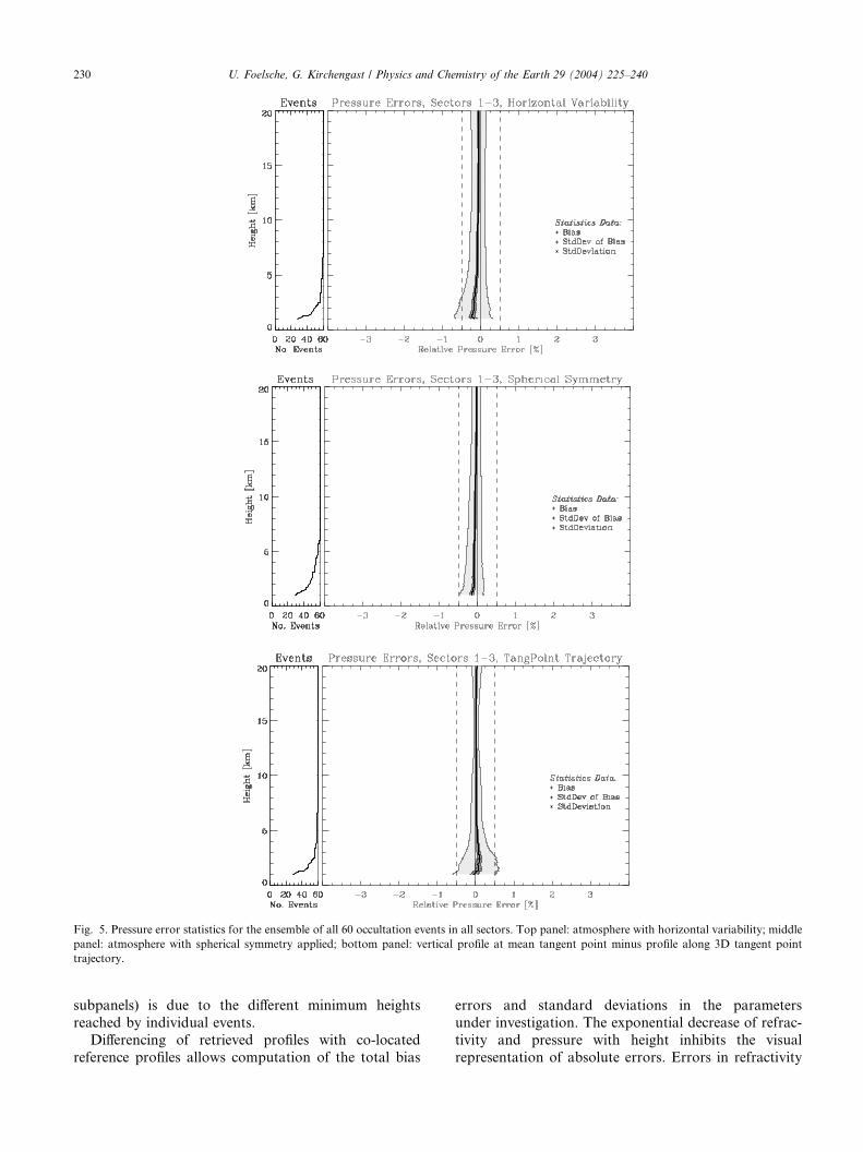
Fig. 5. Pressure error statistics for the ensemble of all 60 occultation events in all sectors. Top panel: atmosphere with horizontal variability; middle

panel: atmosphere with spherical symmetry applied; bottom panel: vertical profile at mean tangent point minus profile along 3D tangent point

trajectory.


subpanels) is due to the different minimum heights

reached by individual events.

Differencing of retrieved profiles with co-located

reference profiles allows computation of the total bias

errors and standard deviations in the parameters

under investigation. The exponential decrease of refrac-

tivity and pressure with height inhibits the visual

representation of absolute errors. Errors in refractivity

Fig. 6. Geopotential height error statistics for the ensemble of all 60 occultation events in all sectors. Top panel: atmosphere with horizontal

variability; middle panel: atmosphere with spherical symmetry applied; bottom panel: vertical profile at mean tangent point minus profile along 3D

tangent point trajectory.


(Fig. 4) and pressure (Fig. 5) are thus shown as rel-

ative errors in units [%], while geopotential height(Fig. 6) and dry temperature errors (Fig. 7) are dis-

played in units [gpm] and [K], respectively. All sta-

tistics are shown between 1 km and 20 km above

(ellipsoidal) surface; dashed vertical lines mark rela-tive errors of 0.5% and absolute errors of 10 gpm and

1 K, respectively.

Fig. 7. Temperature error statistics for the ensemble of all 60 occultation events in all sectors. Top panel: atmosphere with horizontal variability;

middle panel: atmosphere with spherical symmetry applied; bottom panel: vertical profile at mean tangent point minus profile along 3D tangent point

trajectory.


3.1. Refractivity errors

Fig. 4 illustrates that refractivity errors in a hori-zontally variable atmosphere increase considerably

below a height of about 7 km (top panel). In the

spherically symmetric atmosphere (middle panel), the

increase in refractivity error is significantly less pro-

nounced. Above 7 km, the error profiles are quitesmooth. There is a small negative bias of about

0.1%, standard deviations under horizontal variability


(spherical symmetry) increase from �0.2% (<0.1%) at

20 km to �0.4% (�0.1%) at 7 km.

Below 7 km there is considerable structure in the

error profiles. In the spherically symmetric atmosphere,

standard deviations reach maximum values of 0.7% at

heights around 1.5 km, with a maximum (negative) bias

of 0.3%. In the realistic atmosphere, standard deviationsreach a maximum value of 1.8% at 1.8 km height, the

bias slightly exceeds 0.5% around 2.5 km and below 1.7

km.

3.2. Dependence on the geometry of reference profiles

According to Fig. 4 (bottom panel), differences be-

tween ‘‘true’’ vertical profiles at mean tangent pointlocations and ‘‘true’’ ones along actual 3D tangent point

trajectories are very small in the lower stratosphere,

since the EGOPS mean location estimate is designed to

fit best around 15 km. Below 7 km, however, the dif-

ferences are of a magnitude comparable to the errors

estimated under horizontal variability (top panel). This

implies that the geometrical mis-alignment of the actual

tangent point trajectory with the mean-vertical con-tributes as a major source to horizontal variability error.

Additional visual evidence for this is that the bias below

7 km in the lower panel appears roughly mirror-

symmetric relative to the one in the upper panel. This

occurs since the geometrical mis-alignment is a main

bias source in both cases so that a clearly visible effect

left is the change in sign due to the upper panel using the

mean-vertical profile as reference while the lower paneluses the along-trajectory one.

This finding applies also to the other parameters

(Figs. 5–7) and indicates the importance of utilizing

tropospheric RO profiles not just vertically but as good

as possible consistent with the actual tangent point

trajectory (or, more generally, occultation plane move-

ment). Overall, the results show that the performance in

the realistic horizontally variable troposphere is mark-edly improved if measured against the actual tangent

point trajectory.

3.3. Pressure errors

The pressure errors (Fig. 5) display a similar behavior

as the refractivity errors, though the smaller-vertical-

scale variations are less pronounced due to the hydro-static integration.

In the spherical symmetry case, all relative errors

increase with decreasing height (bias from 0.1% to

0.2%, standard deviation from 0.2% to 0.34%). In the

realistic atmosphere with horizontal variability, stan-

dard deviations are smallest around 13 km height

(0.2%), below they increase up to �0.5% around 1.3

km height, where the negative bias also has its maxi-mum value of �0.2%.

3.4. Geopotential height errors

Errors in the geopotential height of pressure surfaces

are shown in Fig. 6 as function of pressure height zp (a

convenient pressure coordinate defined as zp ¼ �7 � lnp [hPa]/1013.25), which is closely aligned with height z).Mirroring the pressure errors (see, e.g., Syndergaard,1999, on the relation between pressure and geopotential

height), positive biases in geopotential height corre-

spond to negative biases in pressure (cf. Figs. 5 and 6).

In the realistic atmosphere, biases are <5 gpm above

about 7 km, exceed 10 gpm below about 3 km, and

reach a maximum of �13 gpm at �1.3 km pressure

height (corresponding to a pressure error of �0.2%).

Standard deviations are <15 gpm above about 5 km andreach �33 gpm at lowest levels. In the spherically sym-

metric atmosphere, the bias above about 7 km is largely

the same as in the realistic case, but remains <8 gpm

lower down (compared to �13 gpm with horizontal

variability); the standard deviation reaches �20 gpm

(instead of �33 gpm) at lowest levels.

3.5. Temperature errors

The dry temperature errors are depicted in Fig. 7. In

the scenario with horizontal variability, all errors below

7 km are larger than the corresponding errors under

spherical symmetry. A positive bias of �1 K is reached

around 2.6, 1.5, and 1.2 km, respectively, where stan-

dard deviations of about 4 K are encountered.

Under spherical symmetry, the maximum bias is 0.4K at 1.2 km, standard deviations remain smaller than

1.2 K. Between 7 and 20 km there is essentially no

temperature bias in both scenarios (i.e., always smaller

than 0.1 K).

4. Sensitivity to the angle-of-incidence

In this part of the study, the sensitivity of retrieval

products to the angle-of-incidence of occultation rays

relative to the boresight direction of the receiving an-

tenna (aligned with the LEO orbit plane) is analyzed.

Error analyses have been performed for each azimuth

sector (ensembles of 20 events), for every atmospheric

parameter under study. Occultation events in the 0–10�sector are associated with almost co-planar GNSS andLEO satellites, which should lead to the most-vertical

and best-quality occultation events.

Errors in refractivity and pressure, respectively, are––

as in Section 3––displayed as relative values in units [%],

geopotential height and dry temperature errors as

absolute values in units [gpm] and [K], respectively. All

statistics are shown between 1 and 20 km above the

(ellipsoidal) surface; the dashed vertical lines indicate


relative errors of 0.5% and absolute errors of 10 gpm

and 1 K, respectively.

Each of the following figures, Figs. 8–11, shows the

results for sector 1 in the top panel, for sector 2 in the

Fig. 8. Refractivity error statistics for occultation events in sector 1 (top p

middle panel, and for sector 3 in the bottom panel,

respectively (the three sectors are defined as described in

Section 2.1). Refractivity errors are shown in Fig. 8,

pressure errors in Fig. 9, geopotential height errors in

anel), sector 2 (mid panel), and sector 3 (bottom panel), respectively.

Fig. 9. Pressure error statistics for occultation events in sector 1 (top panel), sector 2 (mid panel), and sector 3 (bottom panel), respectively.


Fig. 10, and dry temperature errors in Fig. 11, respec-

tively.

One general result pertains to all parameters studied:

above �5 to 10 km, the behavior of the result profiles

for all parameters is quite similar in that errors increase

with increasing angle-of-incidence. Below these heights

this is only valid with several exceptions, which deserve

further investigation.

Fig. 10. Geopotential height error statistics for occultation events in sector 1 (top panel), sector 2 (mid panel), and sector 3 (bottom panel),

respectively.


4.1. Refractivity errors

The ensemble of 20 occultation events with small

angles-of-incidence (sector 1) has no significant bias (less

than 0.1%) above 10 km height. Standard deviations in

the same height interval are smaller than 0.2%. Between

10 and 2.5 km, bias and standard deviation increase

almost continuously (with decreasing height) to 0.7%

and 1.1%, respectively. Below �2.5 km, the increase is

less uniform. At �1.3 km height bias and standard

Fig. 11. Temperature error statistics for occultation events in sector 1 (top panel), sector 2 (mid panel), and sector 3 (bottom panel), respectively.


deviation reach maximum values of 0.9% and �2%,

respectively.

Events in sector 2 show remarkable features in theheight interval below 10 km: the bias is explicitly smaller

than in sector 1, while standard deviations are of com-

parable size (maximum: �2.3% near 3.5 km). At 4.5 km,

the bias reaches a maximum (negative) value of )0.3%,

below that it oscillates around zero. Below 3.5 km, theerror estimates become smaller again, which roots partly

in the fact that the sample size decreases gradually (see


left-hand side subpanel of middle panel of Fig. 8) leav-

ing a smaller ensemble tentatively composed of more

‘‘well-behaved’’ profiles.

Events with angles-of-incidence between 40� and 50�(sector 3) exhibit an approximately constant negative

bias of about 0.1% above 8 km height, while standard

deviations are markedly larger. The largest biases (near1%) and standard deviations (�2.5%) are encountered at

around 1.5–2 km height.

4.2. Pressure errors

All sectors display (generally very small) negative

biases over the entire height domain. Standard deviation

are smaller than 0.5% almost everywhere; they aresmallest in sector 1, whereas biases are smallest in sector

2.

Occultation events in sector 1 exhibit biases of less

than 0.1% between 6 and 20 km, which are, nevertheless,

slightly larger than corresponding biases in sector 2.

Below 6 km, they gradually increase to �0.2% at lowest

levels. Standard deviations remain smaller than 0.4% at

all heights.Events in sector 2 have the smallest biases in the en-

tire height domain: they are always smaller than �0.1%.

Standard deviations remain almost constant (about

0.2%) down to about 10 km, then they start to increase

gradually but never exceed 0.5%.

Events in sector 3 display a marked (constant) neg-

ative bias of �0.1% between 5 and 20 km height, while

standard deviations amount to about 0.2% (approxi-mately constant as well). Below 5 km, the bias increases

continuously to �0.4%. Standard deviation increase to

�0.6% at lowest levels.

4.3. Geopotential height errors

Geopotential height errors are, as already in Fig. 6 of

Section 3, displayed as functions of pressure height.Positive biases (related to negative pressure biases) can

be detected in all sectors. In line with the pressure error

results they are smallest in sector 2, while standard

deviations are smallest in sector 1.

The bias in sector 1 increases continuously from �1.5

gpm at 20 km to 16 gpm at 1 km pressure height, the

standard deviations from �7.5 to �20 gpm.

Sector 2 has again the smallest bias, the maximum isslightly more than 8 gpm near 2.5 km. Standard devia-

tions grow evenly from �10 gpm at 20 km to �33 gpm

at 1 km.

In sector 3, there is a pronounced positive bias of

about 8 gpm between 20 and 4 km, which increases

downwards to about 25 gpm. Standard deviations rise

from about 20 gpm at 20 km to about 40 gpm at

1 km.

4.4. Temperature errors

The temperature errors (Fig. 11) closely reflect the

overall behavior of the refractivity errors (Fig. 8), though

with a change in sign leading to mirror-symmetry of

temperature vs. refractivity errors. This behavior is

caused by the inverse relation of the two parameters viathe equation of state and was explored in detail by Rieder

and Kirchengast (2001a,b).

Events in sector 1 exhibit very small biases of less

than �0.1 K above 10 km, which slowly (but not uni-

formly) increase to 0.4 K at 4 km and come close to 2 K

at lowest levels. Standard deviations increase from �0.2

K at 20 km to �2.5 K at near 3 km.

Events in sector 2 are practically bias-free between 6and 20 km (biases <0.1 K). Below this height, biases

remain <0.8 K throughout. Standard deviations in this

lower height domain are only slightly larger than in

sector 1.

Events in sector 3, finally, show small biases, never

exceeding 0.1 K, down to about 9 km. Below 4 km,

biases increase markedly and reach a maximum value of

close to 2 K at 2.5 km. Standard deviations are around0.5 K down to 10 km. Below 4 km, there is a pro-

nounced increase of up to �6 K between 1.5 and 2 km

height.

5. Summary, conclusions, and outlook

This study addressed the sensitivity of GNSS ROmeasurements to atmospheric horizontal variability.

Retrieved geophysical parameters from refractivity via

pressure and geopotential height to dry temperature

have been investigated.

The errors in a realistic horizontally variable atmo-

sphere have been compared with errors in a spherically

symmetric atmosphere. This investigation was based on

an ensemble of 60 simulated occultations, using a rep-resentative ECMWF T213L50 analysis field with and

without horizontal variability, respectively. Below �7

km height biases and standard deviations of all consid-

ered atmospheric parameters under spherical symmetry

are significantly smaller than corresponding errors in a

realistic atmosphere with horizontal variability. Tem-

perature standard deviations below 5 km, for example,

remain smaller than 1.2 K in a spherically symmetricatmosphere while they reach values of about 4 K in the

realistic atmosphere. This confirms earlier results based

on a more simplified estimation by Kursinski et al.

(1997), that horizontal variability is an important error

source in the troposphere. Dry temperature profiles

between 7 and 20 km were found to be essentially bias-

free in both the realistic and spherical-symmetry sce-

narios (biases smaller than 0.1 K), which confirms theunique climate monitoring utility of GNSS occultation


data. Small residual biases of �0.2–0.3 K between about

7 and 14 km where found, though, for ensembles of

events at high latitudes within separate parallel work

(Foelsche et al., 2003). Within this study, involving only

about 10 events at high latitudes (poleward of 60�), thatresidual bias was (partly) visible only in the results for

the 0–10� azimuth sector. Nevertheless, it certainly callsfor closer study in the future.

A significant part of the total error below �7 km can

be attributed to adopting reference profiles vertically at

mean tangent point locations (designed to fit best at

heights around 15 km) instead of extracting them along

actual 3D tangent point trajectories through the tropo-

sphere. This finding indicates the importance of utilizing

tropospheric RO profiles as good as possible consistentwith the actual tangent point trajectory (or, more gen-

erally, occultation plane movement). Future work will

investigate this matter more closely based on a larger

ensemble of events and on an even higher-resolved field

(ECMWF T511L60 analysis field). We will also rigor-

ously inspect by how much the standard deviation and

bias errors decrease if the data are exploited along a

tangent point trajectory deduced purely from observeddata, mainly GNSS and LEO satellite position and

bending angle data.

The sensitivity of retrieval products to the angle-of-

incidence of occultation rays relative to the boresight

direction of the receiving antenna was analyzed for three

different azimuth sectors. Below about 7 km, the general

result for all parameters studied is qualitatively quite

clear: most errors were found to increase with increasingangle of incidence. This is in line with the hypothesis

that larger angles of incidence lead to more sensitivity to

horizontal variability. Biases in the 20–30� azimuth

sector are generally smaller than corresponding biases in

the 0–10� sector, however, despite the latter is associatedwith almost co-planar GNSS and LEO satellites, which

should lead to the most-vertical and best-quality occul-

tation events. This may be due to the comparativelysmall number of occultation events in the present study

but certainly merits further investigation. In general, the

sensitivity of bias errors to increases of the angle of

incidence has been found to be relatively small, which is

favorable regarding the climate monitoring utility of the

data. For example, dry temperature biases between 7

and 20 km exhibit no relevant increase with increasing

angle of incidence. Current cautionary approachesrestricting the events used in climate studies to small

angles of incidence (such as <15�; Steiner et al., 2001)

may thus be overly conservative.

Future work needs to further improve the under-

standing of all errors involved, in particular of the

residual biases, in order to eliminate or mitigate them

to the largest extend possible. This will optimize the

climatological quality of the data at all angles of inci-dence.

Acknowledgements

The authors thank A.K. Steiner (IGAM/UG) and S.

Syndergaard (University of Arizona, Tucson, USA) for

support in preparing some auxiliary computer codes

used in the study. The EGOPS software, the core tool of

the study, was developed by an international consortiumled by IGAM/UG and involving partner teams at

Danish Meteorological Institute and TERMA Elektro-

nik A/S, Denmark, the Meteorological Office, UK, and

Austrian Aerospace GmbH, Austria, with the major

funding provided by the European Space Agency. The

European Centre for Medium-Range Weather Forecasts

(ECMWF, Reading, UK) provided the atmospheric

analysis field used. The study was funded by the Euro-pean Space Agency under ESA/ESTEC Contract No.

14809/00/NL/MM. Furthermore, U.F. received financial

support for the work from the START research award

of G.K. funded by the Austrian Ministry for Education,

Science, and Culture and managed under Program No.

Y103-CHE of the Austrian Science Fund.

References

Ahmad, B., Tyler, G.L., 1999. Systematic errors in atmospheric

profiles obtained from Abelian inversion of radio occultation data:

effect of large-scale horizontal gradients. J. Geophys. Res. 104

(D4), 3971–3992.

Foelsche, U., Kirchengast, G., Steiner, A.K., 2003. Global climate

monitoring based on CHAMP/GPS radio occultation data. In:

Reigber, et al. (Eds.), First CHAMP Mission Results for Gravity

Magnetic and Atmospheric Studies. Springer, Berlin.

Gobiet, A., Kirchengast, G., 2002. Sensitivity of atmospheric profiles

retrieved from GNSS occultation data to ionospheric residual and

high-altitude initialization errors. Technical Report for ESA/

ESTEC No. 1/2002, Institute for Geophysics, Astrophysics, and

Meteorology, University of Graz, Austria.

GRAS-SAG, 1998. The GRAS instrument on METOP, ESA/EU-

METSAT Report (ESA No. VR/3021 /PI, EUM.No. EPS/MIS/IN/

9), ESA/ESTEC, Noordwijk, Netherlands, 38p.

Healy, S.B., 2001. Radio occultation bending angle and impact

parameter errors caused by horizontal refractivity index gradients

in the troposphere: a simulation study. J. Geophys. Res. 106 (D11),

11,875–11,889.

Hedin, A.E., 1991. Extension of the MSIS thermosphere model into

the middle and lower atmosphere. J. Geophys. Res. 96, 1159–

1172.

Kahle, H.-G., 1984. Reference ellipsoid and geoid. In: Fuchs, K.,

Stoffel, H. (Eds.), Landolt-B€ornstein Numerical Data and Func-

tional Relationships in Science and Technology. Springer-Verlag,

Berlin. Volume 2, Subvolume A, pp. 332–336.

Kirchengast, G., 1998. End-to-end GNSS Occultation Performance

Simulator overview and exemplary applications, Wissenschaft. Ber.

No. 2/1998, Institute for Meteorology and Geophysics, University

of Graz, Austria.

Kirchengast, G., Fritzer, J., Ramsauer, J., 2001. End-to-end GNSS

Occultation Performance Simulator Version 4 (EGOPS4) Software

User Manual (Overview and Reference Manual), Technical Report

for ESA/ESTEC No. 5/2001, Institute for Geophysics, Astrophys-

ics, and Meteorology, University of Graz, Austria, Available from


<http://www.uni-graz.at/igam-arsclisys/ARSCliSys_papers_en.

html>.

Kursinski, E.R., Hajj, G.A., Schofield, J.T., Linfield, R.P., Hardy,

K.R., 1997. Observing earth’s atmosphere with radio occultation

measurements using the Global Positioning System. J. Geophys.

Res. 102 (D19), 23429–23465.

Rieder, M.J., Kirchengast, G., 2001a. Error analysis for mesospheric

temperature profiling by absorptive occultation sensors. Ann.

Geophys. 19, 71–81.

Rieder, M.J., Kirchengast, G., 2001b. Error analysis and character-

ization of atmospheric profiles retrieved from GNSS occultation

data. J. Geophys. Res. 106, 31,755–31,770.

Salby, M.L., 1996. Fundamentals of Atmospheric Physics. Academic

Press, San Diego.

Smith, E.K., Weintraub, S., 1953. The constants in the equation for

atmospheric refractive index at radio frequencies. Proc. IRE 41,

1035–1037.

Steiner, A.K., Kirchengast, G., Ladreiter, H.P., 1999. Inversion, error

analysis and validation of GPS/MET occultation data. Ann.

Geophys. 17, 122–138.

Steiner, A.K., Kirchengast, G., Foelsche, U., Kornblueh, L.,

Manzini, E., Bengtsson, L., 2001. GNSS occultation sound-

ing for climate monitoring. Phys. Chem. Earth (A) 26, 113–

124.

Syndergaard, S., 1999. Retrieval analysis and methodologies in

atmospheric limb sounding using the GNSS radio occultation

technique. DMI Scient. Report 99-6. Danish Meteorological

Institute, Copenhagen, Denmark, 131p.

http://www.uni-graz.at/igam-arsclisys/ARSCliSys_papers_en.html

http://www.uni-graz.at/igam-arsclisys/ARSCliSys_papers_en.html

sensitivity of gnss radio occultation data to horizontal ...wegc · sensitivity of gnss radio...

Documents