ANNALS OF GEOPHYSICS, 57, 2, 2014, A0215; doi:10.4401/ag-6320

A0215

Sensing the upper and lower levels of the atmosphere during the2009 equinoxes using GPS measurements

Wayan Suparta1,*

1 Universiti Kebangsaan Malaysia, Space Science Centre (ANGKASA), Institute of Climate Change, 43600 Bangi, Selangor,

Malaysia

ABSTRACT

This short-term work characterized the upper and lower levels of the at-mosphere through Global Positioning System (GPS) measurements. Theobservations were conducted during the 2009 equinoxes from two pairs ofconjugate polar observing stations: Husafell, Iceland (HUSA) and Res-olute in Nunavut, Canada (RESO) and their conjugate pairs at Scott Base(SBA) and Syowa (SYOG) in Antarctica, respectively. The total electroncontent (TEC), an indicator of the upper atmosphere, and the precipitablewater vapor (PWV), which served as the lower atmospheric response,were retrieved and analyzed. The results reveal a good relationship be-tween TEC and PWV at each station during the onset day of theequinoxes, whereas an asymmetrical response was observed in the begin-ning of and after the equinoxes. In addition, the conjugate pairs wereonly consistent during the autumnal equinox. Thus, the high correlationwas observed following the seasonal pattern for the onset day, while strongand moderate correlations were found only for the vernal equinox inAntarctica and the Arctic, respectively. This relationship reflects the factthat the intensity of solar activity during the solar minimum incident onthe lower atmosphere through the conjugate points is associated with thevariation of the Sun’s seasonal cycle, whereas the TEC and PWV showedan opposite relationship.

1. IntroductionThe use of the Global Positioning System (GPS) in

a wide variety of applications has exploded in the lastfew years. With the advancement of GPS technologyand the spread of the GPS network around the world toremote locations such as Antarctica, the application ofGPS to tasks including monitoring atmosphere dy-namics, positioning and tracking, meteorology, andgeophysical surveying has become possible. Recently,GPS has become a powerful tool for quantifying theionospheric total electron content (TEC) [e.g., Coco1991, Wanninger 1993, Klobuchar 1996] and the at-

mospheric precipitable water vapor content (PWV)[e.g., Bevis et al. 1994, Businger et al. 1996, Rocken et al.1997] in a cost-effective manner with global coverageand superior temporal and spatial resolution. This ap-plication of GPS can improve our understanding of themechanisms driving ionospheric irregularities and theevolution of water vapor, two important factors in therelationship between solar activity and our atmosphere.Many studies have shown that perturbations in the ion-osphere are clearly related to solar activity [e.g., Per-rone and Franceschi 1998, Liu et al. 2011]. However, theimpact of the ionosphere on the dynamics of Earth’satmosphere is still debated, and the interaction betweenthe ionosphere and the lower atmosphere remainspoorly explained.

To give a clear picture of “upper atmosphere” and“lower atmosphere” in this study, a brief definition isgiven. Scientists have defined both terms in variousways. In the context of meteorology, the “lower atmos-phere” may be described as extending from the plane-tary surface (the troposphere) to the lower stratosphere,where the daily weather evolves. Thus, “upper atmos-phere” refers to the entire region above the troposphere,including the mesosphere, the ionosphere and the ther-mosphere, which are identified by their temperaturestructure, density, composition and degree of ioniza-tion. Alternatively, the atmosphere can be divided intotwo different strata, the neutral atmosphere and theionosphere, by considering the propagation of radiowaves, such as GPS signals. The neutral atmospherelayer consists of three temperature-delineated regions:the troposphere, the stratosphere and part of themesosphere. This layer is often simply referred to as thetroposphere because the troposphere’s effects dominate

Article historyReceived March 30, 2013; accepted March 5, 2014.Subject classification:GPS TEC, PWV, Equinoxes, Conjugate points, Associations.

radio wave propagation. Therefore, to the GPS re-searcher, the “troposphere” generally refers to the neu-tral atmosphere spanning the altitudes of 0 to 40 km[Gregorius and Blewitt 1999]. Thus, when speaking ofthe ionosphere, the term refers to anything above thetroposphere layer, or the upper part of the atmosphere.According to the subdivisions of the atmosphere pro-posed by Seeber [1993], the ionosphere is a conductinglayer of weakly ionized plasma in the Earth’s upper at-mosphere. It stretches from approximately 50 to 1500km above the Earth’s surface and contains a significantnumber of ionized particles, i.e., free electrons and pos-itively charged ions. Technically, because the iono-sphere is a dispersive region of the Earth’s atmosphere,TEC is the parameter that most affects a GPS signalalong its trajectory from each satellite to the observer.Thus, in this context, the term “upper atmosphere”refers to the ionosphere, which has characteristics thatare substantially influenced by the Sun. Conversely, theterm “lower atmosphere” refers to the troposphere,where PWV is the climatic parameter that significantlyaffects GPS signals.

Along with the upper atmosphere’s characteristics,the seasonal behaviors of the ionosphere have been in-vestigated for several decades, but the differences in theionosphere between the March and September equinoxesare still open for discussion [Liu et al. 2010]. This workcharacterized the upper and lower levels of the atmos-phere using measurements obtained from ground-based GPS receivers during the 2009 equinoxes. Duringthe equinox periods, the Sun moves northwards alongthe ecliptic in March and southwards in September; theequinoxes are better understood as the times when theday and night last almost exactly 12 hours. Because thecharged particles in the Earth’s magnetosphere tend tobe trapped on the same geomagnetic field-line [e.g.,Dragt 1965], conjugate points between regions couldbe strongly affected by solar activity. Conjugate stationsenable us to investigate the similarities and/or asym-metries of charged particle properties, as well as phe-nomena between the hemispheres [Suparta et al. 2009].Although the altitude between 40 km and 100 km iscomplex, a possible link between the upper and lowerlevels of the atmosphere through the correlation be-tween TEC and PWV at bipolar conjugate points is pro-posed. The analysis is assumed to be valid because themajority of the GPS signal delay occurs when the signaltraverses the ionosphere and troposphere.

2. Measurements and data analysisThis study presents the characterization of solar

activity and terrestrial response during the Vernal Equi-nox (VE) and Autumnal Equinox (AE) periods. Data

collected during the 2009 campaign in Iceland coincidedwith a minimum of solar activity and were processedto clarify the interaction between the upper and loweratmospheres from a GPS perspective. The observationperiods selected were March 6 to April 3 for VE andSeptember 8 to October 6 for AE and were equivalentto two weeks before and after the onset days of theequinoxes. The onsets of VE and AE for 2009 occurredon March 20 at 11:44 UT and on September 22 at 21:18UT, respectively. At these times, the earth receivesmore direct solar energy and most likely experiencesless atmospheric filtering due to the shorter solar dis-tance from the Earth. Accordingly, the observationsof vertical TEC (TEC for simplicity) and PWV areconducted at two pairs of GPS stations located nearmagnetically conjugate points in the Polar Regions.The GPS stations shown in Figure 1 are located atHusafell station (HUSA) in Iceland and Canadian Res-olute (Cornwallis Island) station (RESO), Nunavut.

The two stations in the Northern Hemisphere (NH) formconjugate pairs with Syowa station (SYOG) and ScottBase station (SBA) in Antarctica (Southern Hemisphere,SH), respectively. Table 1 presents the geographical andcorrected geomagnetic coordinates of both GPS conju-gate stations and the instrument setup. The difference incorrected geomagnetic latitude (CGMLat) between theconjugates was approximately 5-10 degrees. Despite thedifference in CGMLat, HUSA-SYOG and SBA-RESO areideal conjugate-pair observatories on the ground in theauroral zone, even though the real conjugate point is onlyfound by the Aurora conjugate [Sato et al. 1998].

The GPS receiver at Husafell (HUSA), Iceland(Table 1) was installed on September 6, 2008. The GPSat HUSA consists of a GPS receiving system and aground-based meteorological system. The GPS re-ceiver consisted of a Leica GRX1200 GG Pro referencestation from the Leica Geosystems, Switzerland withhigh dual-frequency performance, an AT504 choke-ring

SUPARTA

2

Figure 1. Location of GPS stations between the hemispheres withtheir conjugate points. The figures are adapted from http://gdl.cdlr.strath.ac.uk/scotia/vserm/vserm0103.htm.

3

antenna and a notebook included in the Leica GPS Spi-der software for data logging. The dual-frequency LeicaChoke-ring antenna was fully equipped with a DorneMargolin with weather-protection radome. The ground-based meteorological system uses Paroscientific broad-band MET4A sensors, which were installed co-locatedwith the GPS antenna to precisely measure the surfacepressure (in bars), air temperature (in degrees Celsius)and relative humidity (in percent). The GPS antennaand MET4A sensors were fixed on the ground in a basepillar with a height of 5.20 m. The meteorology andthe GPS systems are integrated; thus, the GPS data inthe RINEX folder consisted of observation (∗.obs),navigation (∗.nav) and meteorological data (∗.met)files. The GPS receiver at SBA was installed in Novem-ber 2002 (see the report of Suparta et al. [2008] for moredetails). The GPS data for SYOG and RESO were down-loaded from the GARNER archives at the SOPAChomepage (http://sopac.ucsd.edu).

The geodetic GPS receivers generally collect dual-frequency data at 30 s intervals. To obtain the absoluteTEC and PWV values, the GPS data were convertedand checked using the Translate/Edit/Quality Check(TEQC) routine developed by UNAVCO (http://www.u-navco.org). In this work, geometry-free linear combi-nations of measurements from the same dual-frequencysatellite, such as (Φ1−Φ2) or (P1−P2), were used to esti-mate the variations in the inter-frequency ionospheredelays. With this approach, the TEC measured fromdual-frequency code and phase measurements can becalculated using (1) [e.g., Ephishov et al. 2000, Warnantand Pottiaux 2000, Hofmann-Wellenhof et al. 2001].

The geometry-free linear combination of dual-fre-quency code and phase measurements as a function ofTEC can be calculated using (1)

The ambiguity term can be resolved by combin-ing the geometry-free code with phase measurementsfor each satellite path using (2)

The equivalent vertical TEC (VTEC) can be ob-tained for each satellite path using (2) and (3)

where Prs (L1) and Pr

s (L2) are GPS P-code in meters,Φr

s (L1) and Φrs (L2) are carrier phase in cycles, Dgr and

Dgs are the receiver and satellite differential groupdelay, Nr

s is the ambiguity term in cycles, m1 is thewavelength of the frequency ƒ1 in meters, i and | arethe elevation angles in degrees at the receiver site andat the ionospheric pierce point (IPP), respectively, andhm is the height at sub-ionospheric points. This heightwas set to 400 km, approximately corresponding to thealtitude of maximum electron density. RE is the radiusof the Earth and is taken as 6,378,137 meters. The ab-solute GPS TEC results are then corrected using satel-lite and receiver bias values from the nearest GPSstations available from the data center of Bern Univer-sity, Switzerland. For example, the equivalent GPS sta-tion for Scott Base (SBA) is the GPS station atMcMurdo (MCM4).

For the lower atmosphere, the PWV total is deter-mined from the GPS signals and the surface meteoro-logical data. The total tropospheric delay in the zenithdirection can be formulated as

and

1cos

coscos

VTEC TEC

h R1

rs

rs

m E2

2 1 2i|

|=

= -+^ h

c m

( 1) ( 2) and( 1) ( 2)

P P L P LL L

rs

rs

rs

rs

rs

rsU U U

= -

= -

. ( ) and.

P TEC Dg DgTEC N

0 1050 552

rs

rs

rs

rs

rs

rsU

=

=

- + -

- +

( )P Dg Dg Nrs

rs

rs

rs

1 1m mU- = - -

ZTD ZHD ZWD= +

SENSING THE UPPER AND LOWER ATMOSPHERE

Station(Region)

Glat(Deg)

Glon(Deg)

Height(m)

CGMlat(Deg)

CGMlon(Deg)

Type of GPSreceiver and

year installed

Cutoff elev. angle

UTC Time

HUSA 64.67°N 21.03°W 220.20 61.55 100.57 Leica GRX1200 15° LT=UT

(Arctic) Pro (2008)

SYOG 69.00°S 39.58°E 45.00 66.31 72.22 Trimble 4000SSI 10° LT+12

(Antarctica) (2002)

SBA 77.85°S 166.76°E 15.90 79.93 327.07 Trimble TS5700 13° LT+12

(Antarctica) (2002)RESO 74.69°N 94.83°W 19.98 82.83 323.11 Ashtech UZ-12 0° LT–5(Arctic) (2006)

Table 1. The geographic (G) and the corrected geomagnetic (CGM) coordinates (calculated based on the IGRF/DGRF model for year2009) and instrument setup at two pairs of bipolar conjugate points.

∗D/IGRF stand for the Definite/International Geomagnetic Reference Field

(1)

(5)

(2)

(3)

(4)

where ZTD is the zenith tropospheric delay in the equi-librium state as a function of slant delays and mappingfunctions. The zenith hydrostatic delay (ZHD) is adelay component caused by the dry gases in the tropo-sphere and the non-dipole component of water vaporrefraction. The zenith wet delay (ZWD) is a delaycaused solely by the components of the dipole momentand dipole orientation of water refraction. The ZTD inthis work was estimated based on the improved Modi-fied Hopfield model, which can be expressed as [Hof-mann-Wellenhof et al. 2001, Suparta et al. 2008]

where

and

where the parameters in the brackets are a solutionof the mapping function in the form of a series ex-pansion, aj,k with k denoting the layer. Subscript j isreplaced with h for the hydrostatic component, andsubscript j is replaced by w for the wet component. In(7), hj (in meters) represents hh (hh=40136+148.72T)and hw (set to 11 km), which are the effective heightsfor the hydrostatic and wet components, respectively,and rj is the solution model of the integral that coversthe hydrostatic and wet portions of troposphericdelay. Nj,0

Trop is the total refractivity at the surface of theEarth.

The ZHD is calculated using the Saastamoinenmodel [Saastamoinen 1972]. ZHD uses the surface pres-sure (P) measurements and a correction factor to cor-rect the local gravitational acceleration at the center ofmass of the atmospheric column, which can be ex-pressed as follows and has a value close to unity:

where m is the station latitude (in degrees) and h is theheight of the site above the ellipsoid (in km) as meas-ured by the GPS receiver.

In this work, the hydrostatic Vienna Mapping Func-tion (VMF1) mh(i) is employed to reduce the depend-ence of the zenith delay (ZTD) on the satellite elevationangle. This mapping function uses the European Centrefor Medium-Range Weather Forecasts (ECMWF) in-stead of the Numerical Weather Models (NWMs) be-cause of its greater sensitivity and suitability for PolarRegions and is written as

where the coefficients a, b and c are interpolated fromthe latitude of the GPS site and take seasonal varia-tions into account. Boehm et al. [2006] has updated the“b” and “c” coefficients of the Marini continued frac-tion form in (9). Here, f (i,aht, bht, cht) represents thethree-term continued fraction in the Marini mappingfunction:

The coefficients aht= 2.53 × 10-5, bht= 5.49 × 10-3

and cht= 1.14 × 10-3 were determined by a least-squaresfit to the height corrections at nine elevation angles.

When ZTD was mapped onto the satellite eleva-tion angle using the VMF1, the ZWD was then calcu-lated by subtracting the ZHD from the ZTD (seeEquation 5). The PWV can now be calculated as pro-posed by Bevis et al. [1994]

where the dimensionless r(Tm) parameter is a conver-sion factor that varies with the summation on the localclimate (e.g., location, elevation, season and weather)and depends on a weighted mean temperature (Tm), asgiven by

where ρlwand Rv are the density of liquid water (1000kg m-3) and the specific gas constant for water vapor(461.5184 J mol-1 K-1), respectively. According to (12),kˈ2 and k3 are the refraction constants: kˈ2=(22.1±2.2)

ZTD N k r10 ,,

jTrop k j

jk

k

60

1

9 a= -

=

; E/

1

6 4

4

12 6

4

4

4

a b

a a b

a a b

a b a b

b a b

a b

b

a

b

3

6 4

3

,

,

,

,

,

,

,

,

,

j

j

j j j

j j j j

j j j j j

j j j j j

j j j j

j j j

j j

j

1

2

2

2 2

2

2 2

2

3

4

54

6

7

83

94

a

a

a

a

a

a

a

a

a

=

=

= +

= +

= + +

= +

= +

=

=

^

^

^

^

^

h

h

h

h

h

, 2 ,sin cos

cos sin

a h b h R

r R h RR

jj

jj E

j E j EE

2

2 2

i i

i i

=- =-

= + - -^ ^h h

(1 0.00266 (2 ) 0.00028 )( . . )

cosZHD hP2 2768 0 0024!

m= - -

( ) ( ) ( )

( )( ( ))

, , ,

sin sin sin

sin

m m m

a b ca b c

f a b c h

1 1 1

1

h

ht ht ht

i i i

i i i

i i

D= + =

=+ + +

+ + ++

+ -

^

^

^

h

h

h8 B

, , ,

( ( ))( (1 ))

sin sin sin sin

f a b c

a b ba b c1 1

ht ht ht

ht ht ht

ht ht ht

i

i i i i=

+ + + +

+ + +

=^

^

^

h

h

h

PWV T ZWDmr= ^ h

T TR k k 10m mlw v 2 31 6r t= + -l^ ^h h6 @

SUPARTA

4

(6)

(7)

(8)

(9)

(10)

(11)

(12)

5

Kmb-1 and k3=(3.739±0.012) × 105 K2 mb-1. The meantemperature Tm is estimated linearly [Bevis et al. 1994]:

where TK is the surface air temperature in Kelvin. TheGPS PWV has been compared with the PWV from Ra-diosonde [Suparta 2010], and it was found that the Ra-diosonde PWV in the Polar Regions is not significantlydifferent (less than 2%) from the mid-latitude region.Thus, Tm is calculated from the surface temperature (T)measured at a particular site. The r(Tm) value for PolarRegions ranges between 0.14-0.15, which is lower by ap-proximately 3% than the value in the mid-latitude region.

Assuming that all the instrumental biases can be iso-lated through the use of differencing techniques and by si-multaneously reducing the satellite orbit errors, theremaining errors are expected to be only caused by ionos-pheric and tropospheric influences. In addition to the in-strumental effects, the removal of the ionospheric delayeffects from the GPS processing is required to determinethe total ZTD. A Matlab program suite, namely, the tro-pospheric water vapor program (TroWav), was developedto process and analyze all of the above parameters. De-

tailed algorithms for TroWav used in this work can befound in Suparta et al. [2008] and Suparta [2010]. The GPSTEC measurements at all stations were collected at 30 sintervals. The GPS PWV results for all stations were cal-culated following the interval in the meteorological data.Thus, the PWV products for HUSA, SBA, RESO andSYOG were generated with 1-min, 10-min, 1 h and 3 h in-tervals, respectively. To analyze the equinoxes at all sta-tions, the data were averaged with interval of 15 min forGPS TEC and 3 h for GPS PWV. Approximately onemonth (two weeks before and after the equinox onsets)of data for the TEC and the PWV at two pairs of conju-gate stations, as well as solar activity, were analyzed. Theanalysis consisted of correlating the TEC and PWVmeasurements. This correlation analysis was selected asthe best method of determining the association betweentwo unknown variables.

3. Results and discussion

3.1. Solar activity during the 2009 equinoxesFigure 2 shows the solar and geomagnetic activity

during the 2009 equinoxes for both VE and AE. Thesunspot number (SSN) on the top panel was recorded

. .T T70 2 0 72m K= +

SENSING THE UPPER AND LOWER ATMOSPHERE

Figure 2. Solar-geomagnetic activity during the 2009 equinox periods. The vertical dashed lines denote the vernal equinox (VE) onset onMarch 20 at 11:44 UT and the autumnal equinox (AE) onset on September 22 at 21:18 UT. The date marked on the figure is in dd/mm for-mat. The sunspot number (SSN), the 3-hour Kp and the daily Ap indices were obtained from the NOAA/SEC website (http://www.swpc.noaa.gov), and hourly Dst (nT units) was obtained from the World Data Center-C2 for geomagnetism, Kyoto (http://wdc.kugi.kyoto-u.ac.jp).

(13)

as a maximum of 12 before VE and 32 after AE. The ge-omagnetic conditions shown in the second and thirdpanels are categorized as low activity with four minor-to-unsettled storms (3 h Kp>4, 8<Ap<16) and one stormwith a minimum disturbance storm time (Dst) of −31nT that occurred on March 12. The Dst is an index thatis commonly used to identify and quantify magneticstorms as a reflection of the level of magnetospheric en-ergy input to the upper atmosphere based on groundmeasurements. The maximum 3-h value of the aa indexof 46 nT (bottom of Figure 2) was recorded for the VEand AE periods that occurred 8 days before and 5 daysafter the onsets of VE (Ap=16 nT) and AE (Ap=8 nT),respectively. Similar to the Ap and Kp indices, the aaindex was used as a proxy for solar irradiance linkingto the Earth’s climate through terrestrial surface tem-perature records [Cliver et al. 1998]. At the onset of VEon March 20, Ap and aa indices were recorded at lowvalues of 4 and 8 nT, respectively, with a Dst of 2 nT.Note that increases in the geomagnetic activity wereobserved on March 12 and 21, perhaps due to thetopology of the geomagnetic field at ground level. Itis interesting to note that at the onset of AE on Sep-tember 22, all recorded values of geomagnetic activ-ity were low, which is similar to the observations atthe onset of VE. Subsequently, SSN reached a maxi-

mum of 32 on September 24, followed by increasesof geomagnetic activity between September 27 and28. Overall, low solar activity was observed duringthese equinoxes, and their conditions can be catego-rized as quiet.

3.2. TEC and PWV observations during the 2009equinoxes

In the following section, the analyses of TECand PWV during the 2009 equinoxes will be pre-sented according to (1) variation in the two weeks be-fore and after the equinoxes and (2) the onset day ofequinox.

3.2.1. TEC responseFigure 3 shows the one-hour average of TEC varia-

tion for two weeks before and after the equinoxes. TheTEC exhibits a diurnal pattern with different oscillatorypatterns at different stations. For VE, HUSA-RESO ex-hibited a stable fluctuation, while SYOG and SBA exhib-ited fluctuations one week before the onset of VE andthen increased trend. In certain periods, SBA was foundto lack GPS data for VE and AE, and thus, the responseof the SBA-RESO pair will be approximated. The TECvariation at the onset of VE and AE exhibited oppositepatterns in the two hemispheres for both station pairs.

SUPARTA

6

Figure 3. The TEC variation at both conjugate pairs for a 14-day period before and after the (a) vernal equinox (VE) and (b) autumnal equi-nox (AE), respectively. The vertical dashed line indicates the onset.

7

One pattern observed at the paired stations is that of solarinfluence: the SH received less light and exhibited reducedTEC, while the NH received more light and exhibited in-creased TEC. There is not a clear signature of interhemi-spheric influences (either similarity or asymmetry),particularly during VE. Thus, spatial TEC variation duringequinoxes seems influenced by seasonal dependencies.

To compare the TEC variation during the onset ofequinox, 2 hours of TEC map structure during VE(March 20) and AE (September 22) are presented in Fig-ure 4. The geographic longitudes (GLon) depicted in thefigure are assumed to be close to the values for HUSA(−20.0°), SYOG (40.0°), RESO (−95.0°) and SBA(170.0°). The values are approximate because NASA’scrustal dynamics data interchange system (CDDIS) onlyprovides TEC values at 5 degree intervals. For both VEand AE at all stations, HUSA-SYOG (at the top two pan-els in Figure 4) exhibited higher TEC during the mid-day,whereas SBA-RESO (at the bottom two panels in Figure4) exhibited lower TEC in the mid-night. The stations inthe NH (HUSA and RESO) and in the SH (SBA andSYOG) are arranged in a rough triangle, differentiatedonly slightly by the shape and distribution of TEC. OnlySBA (GLon: 170.0°) has a different distribution betweenVE and AE, in which the TEC duration during AE in themorning is double than that of VE. Comparing to Figure4b, the slight TEC movement can be clearly observed,with a similar pattern following the seasonal trend.

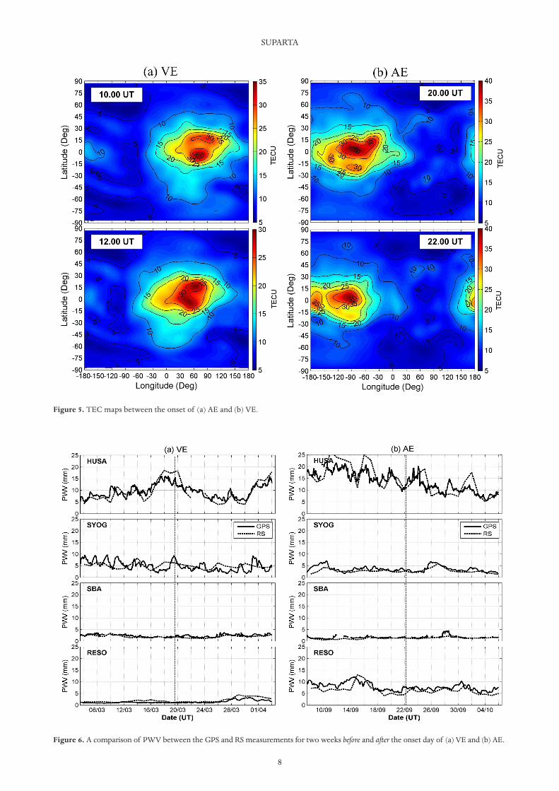
With regard to the onset of VE and AE, Figure 5shows the TEC map for VE between 10:00 UT and12:00 UT and for AE from 20:00 UT until 22:00 UT. At10:00 UT on March 20, the TEC exhibited higher valuesbetween ±15° latitude and 20-90° longitude. The TECthen moved toward the equator (reduced) at 22:00 UT.

At 20:00 UT on September 22, the TEC exhibitedhigher values between −10° and +15° latitude and−30° and −120° longitude. The TEC then moved to-ward the pole (enhanced) at 22:00 UT. One can con-clude from the TEC movement during the onset of VEand AE that the seasonal cycles in the polar and tem-perate zones of one hemisphere are the opposite ofthose in the other hemisphere. When it is summer(more sunlight received) in the NH, it is winter (lesssunlight received) in the SH, and vice versa. From theperspective of a given geographical longitude (GLon),the TEC exhibits positive (higher) values during VE andnegative (lower) values during AE, and vice versa.

3.2.2. PWV responseFigure 6 shows the hourly average temporal PWV

variation for 14 days before and after both VE and AE atbipolar conjugate points. In addition to the validation ofthe GPS PWV, daily averages of PWV from Radiosonde(RS) are presented. The RS PWV data were taken fromthe Wyoming University website. Note that the equiva-lent to the GPS at HUSA is the RS at BIKF (station num-ber (S/N): 4018, location: 63.96°N, 22.60°W at anelevation of 54.0 m); the equivalent to the GPS at SBA isthe RS at McMurdo (S/N: 89664, location: 77.85°S,166.66°E at an elevation of 24.0 m); the equivalent to theRS at RESO is the RS at YRB (S/N: 71924, location:74.70°N, 94.96°W at an elevation of 40.0 m); and theequivalent for SYOG is 89532 (location: 69.00°S, 39.58°Eat an elevation of 21.0 m). Considering the differencesbetween GPS and RS position, only HUSA and KIBF areseparated by a relatively long distance (~100 km).

Across all stations, the PWV values from GPS andRS exhibited a positive linear trend and agreed very

SENSING THE UPPER AND LOWER ATMOSPHERE

Figure 4. TEC maps for each station with geographical longitude (GLon) during the onset day of (a) VE (March 20) and (b) AE (September 22).

SUPARTA

8

Figure 5. TEC maps between the onset of (a) AE and (b) VE.

Figure 6. A comparison of PWV between the GPS and RS measurements for two weeks before and after the onset day of (a) VE and (b) AE.

9

well. For the HUSA station, the PWV values werehigher than for other stations. The conjugate pair ofHUSA-SYOG in Figure 6a shows more fluctuation thanthe pair of SBA-RESO. On the VE onset day, the pair ofHUSA-SYOG exhibited a PWV value approximately 6.4mm higher than their average value (~7.2 mm). For AEin Figure 6b, the PWV at HUSA exhibited a decreasingtrend, whereas the other three stations exhibited lowfluctuations. However, there are two high peaks ofPWV at each station, which alternate every two daysand oscillate when the angle approaches 30° (for ex-ample, on September 24 at HUSA, September 26 atSYOG, September 28 at SBA and September 31 atRESO). The occurrence of these oscillatory peaks be-fore and after the AE onset day is a unique phenomenoncaused by the daily variation of the station. Convinc-ingly, the PWV value for the SH stations was one-thirdlower than for the stations in the NH. The high PWVvalue observed in the NH is possibly due to the Arcticsurface being more explored than the SH. The PWVcan clearly be seen to increase at the onset of VE forHUSA-SYOG, whereas the opposite trend is shown forthe AE onset. In general, the PWV response in the con-jugate pairs for both VE and AE will be stronger whenthe sun is more exposed.

Figure 7 shows the spatial variation of PWV withlatitude: 45° to 90°N/S and longitude 0° to 100°W(NH) and 30° to 180°E (SH) during the VE and AE atfour selected stations. Each station in the figure ismarked by a solid red circle. The PWV map (in mm) isgenerated based on 4-times daily observations at the

surface level from the NCEP/NCAR Reanalysis 1.From both figures, the PWV at RESO and SBA duringVE is estimated to be ~2 mm (shown by green color).However, the PWV at HUSA is estimated to be dou-ble (~6 mm) that of the PWV at SYOG. The high valueof PWV at HUSA is consistent with Figure 6a. For thecase of AE, SBA-RESO and HUSA-SYOG showed anti-correlation, whereas PWV was similar in both hemi-spheres. The low PWV value during AE in the NHstation is due to the seasonal dependence. This sea-sonal phenomenon is a result of the Earth‘s axis beingtilted to relative to its orbital plane (the elliptical orbitof Earth). When the center of the Sun is above thehorizon, its lower edge is visible. In other words, theArctic region experiences a high density of incidentrays, while the other side (the Antarctic region) expe-riences a low density of incident rays. Hence, the sea-sonal cycle in the polar regions of one hemispherewould be opposite to that of the polar regions of theother hemisphere. This condition greatly affects thePWV movement between the poles.

3.2.3. Associations between the upper and loweratmosphere

The associations between the upper and lower lev-els of the atmosphere evident from the TEC and PWVobservations (shown in Figures 3 and 6) at the conjugatestations are presented in Figure 8. The TEC and PWVrelationship is characterized by a correlation coefficient(r), which is calculated at the 99% confidence level foreach station and presented in the associated figures. The

SENSING THE UPPER AND LOWER ATMOSPHERE

Figure 7. Spatial PWV variation for the onset day of (a) VE (March 20, 2009) and (b) AE (September 22, 2009) courtesy of NOAA.

autocorrelation in the data series was taken into accountwhen establishing the statistical significance. During theVE, the bipolar stations exhibited complicated trendswith ups and downs for each station. For example, the

pairs of HUSA-SYOG and SBA-RESO show an oppositetrend before the VE onset day, while after VE, all stationstend to increase. However, it should be noted that thereis no correlation for before and after the VE onset day

SUPARTA

10

Figure 8. Association between TEC and PWV variations at bipolar conjugate stations for (a) VE and (b) AE before, during the onset day andafter the equinoxes.

11

across all of the stations. At the onset day of VE, a goodTEC and PWV relationship was found at all stations: thepair of HUSA-SYOG shows an upward trend, whereasSBA-RESO showed the opposite.

Similar plots are shown for the AE. Before the onsetday, the stations’ trends are similar to those recordedfor VE. The figure also shows that there is no relation-ship between TEC and PWV for all stations. However,anti-correlation between the stations in the NH and SHwas observed after the AE. At the onset day of AE,HUSA-SYOG and SBA-RESO showed anti-correlation,which is dissimilar to the onset day of VE. Generallyspeaking, the correlations between TEC and PWV dur-ing the onset day (equinox) exhibit opposite trends forthe HUSA-SYOG and SBA-RESO pairs. This is due tothe equinox signal that is observed moving from the be-ginning of spring in the NH and autumn in the SHwhen the sun crosses the celestial equator going fromsouth to north. Therefore, the Antarctic station receivesthe sun rays before the station in the NH. As a result,the explanation is the same as in Section 3.2.2, wherethe high and low values of the TEC and PWV aregreatly dependent on the seasonal difference betweenthe hemispheres. Thus, the association between theupper and the lower levels of atmosphere through be-havior of both TEC and PWV respond to the sun atbipolar conjugate pairs during a low solar activity is ob-served complexes that physically difficult to explain, al-though good correlation was observed during the onsetday for each station.

4. Summary and conclusionThe characterization of the interhemispheric con-

jugate effects in terms of TEC and PWV variations dur-ing equinoxes has been conducted at pair stations:HUSA-SYOG and SBA-RESO in the Polar Regions.Analyses for before, after and the onset day of both VE andAE during 2009 are summarized as follows.

First, the TEC and PWV variations before and afterthe equinox between the hemispheres were both asso-ciated with normal day-to-day variability of the middle-to-high latitude ionosphere (with some triggeringdisturbed conditions, as evident in Figure 2) and to nor-mal weather variability, respectively. However, both pa-rameters showed fluctuations and diversity, especiallyPWV, which has an indistinct pattern. The difference inTEC peaks can be expected due to daily variations be-tween the stations. The PWV variation does not closelyfollow the TEC patterns, which indicates that the inter-face between the troposphere and the bottom of theionized atmosphere is complex. HUSA station recordeda higher amount of PWV compared to RESO due to itslocation in the Arctic Circle, which passes through the

Arctic Ocean. Second, the relationship between TECand PWV for before and after both the VE and AEshowed a similar lack of correlation. At the onset day ofthe equinoxes, the quantity in the SH station was anti-correlated with that of the station in the NH. Overall,the conjugate pairs of stations show a consistent corre-lation during the AE, but the case of HUSA-SYOG dur-ing the VE is unusual. In other words, a high correlationwas observed to follow a seasonal pattern in each hemi-sphere; during VE, a strong correlation was found inAntarctica (rSBA-SYOG= 0.71) and a moderate correlationwas found in the Arctic (rHUSA-RESO= 0.53), and viceversa for the AE (rHUSA-RESO= 0.83 and rSBA-SYOG= 0.51).These findings clearly demonstrated that the hemi-sphere experiences summer at perihelion and winter ataphelion, implying that the TEC value was clearly in-fluenced by solar activity. Third, the intensity of thesolar radiation incident on the lower atmosphere overthe Antarctic region and its weakness at the conjugatedayside station are noticeable and correspond to thepresence of seasonal effects. Between the hemispheres,both quantities are clearly shown to exhibit oppositepatterns (asymmetries).

In conclusion, the relationship between TEC andPWV during the equinoxes within the solar minimumcondition is expected to be asymmetrical. Asymmetriesare hemisphere-dependent, and higher TEC values canbe recorded during the AE and VE for the SH and NH,respectively. However, it is difficult to characterize thePWV response at the conjugate points because the in-terhemispheric effects are more strongly affected by theupper atmosphere (i.e., TEC variation). The TEC effectson water vapor movement are expected to vary becauseof the different effects on the propagation media. Stronggeophysical disturbances or extreme atmospheric eventscan be proposed for further comprehensive studiesaimed at better understanding the coupling process be-tween the upper and lower levels of the atmosphere. Inaddition, ancillary data from different sources areneeded to support the interpretation of the GPS-basedmeasurements.

Acknowledgements. This work was supported by the Min-istry of Higher Education Malaysia (MOHE) under grant UKM-LL-07-FRGS0211-2010. The author acknowledges the NationalInstitute of Polar Research (NIPR) Japan and Science Institute ofUniversity of Iceland (SIUI) for the collaboration, the Scripps Orbitand Permanent Array Center (SOPAC) for archived GPS data,NASA’s crustal dynamics data interchange system (CDDIS) forTEC map data, the National Oceanic and Atmospheric Adminis-tration (NOAA) for archiving the PWV map data and WyomingUniversity for PWV Radiosonde data. The author would like to ex-press his gratitude to Snorri Johannesson for maintaining the GPSsystem in Iceland during the campaign and give special thanks toFaizatul Noor Abu Bakar and Fadzlina Aini Mohd Lehan for con-tributing to the data processing.

SENSING THE UPPER AND LOWER ATMOSPHERE

ReferencesBevis, M., S. Businger and S.R. Chiswell (1994). GPS

meteorology: Mapping zenith wet delays onto pre-cipitable water, J. Appl. Meteorol., 33, 379-386.

Boehm, J., B. Werl and H. Schuh (2006). Tropospheremapping functions for GPS and very long baselineinterferometry from European Centre for Medium-Range Weather Forecasts operational analysis data,J. Geophys. Res., 111, B02406, doi:10.1029/2005JB003629.

Businger, S., S.R. Chiswell, M. Bevis, J. Duan, R.A. An-thes, C. Rocken, R.H. Ware, M. Exner, T. van Hoveand F.S. Solheim (1996). The promise of GPS in at-mospheric monitoring, Bull. Amer. Meteorol. Soc.,77, 5-18.

Cliver, E.W., V. Boriakoff and J. Feynman (1998). Solarvariability and climate change: geomagnetic and aaindex and global surface temperature, Geophys.Res. Lett., 25, 1035-1038.

Coco, D. (1991). GPS satellites of opportunity for ionos-pheric monitoring, GPS World, 47-50.

Davies, K., and G. K. Hartmann (1997). Studying theionosphere with the Global Positioning System,Radio Sci., 32, 1696-1703.

Dragt, A.J. (1965). Trapped orbits in a magnetic dipolefield, Rev. Geophys., 3, 255-298, doi:10.1029/RG003i002p00255.

Ephishov, I.I., L. W.Baran, I.I. Shagimuratov and G.A.Yakimova (2000). Comparison of total electron con-tent obtained from GPS with IRI, Phys. Chem. Earth,25, 339-342.

Gregorius, T.L.H., and G. Blewitt (1999). Modelingweather fronts to improve GPS heights: A new toolfor GPS meteorology? J. Geophys. Res. B: Solid Earth,104, 15261-15279.

Hofmann-Wellenhof, B., H. Lichtenegger and J. Collins(2001). Global Positioning System: Theory andPractice. Springer Verlag: 5th revised edition, Aus-tralia: Springer-Verlag Wien New York.

Klobuchar, J.A. (1996). Ionospheric effects on GPS inGlobal Positioning System: Theory and Applica-tions, Chapter 12, Parkinson, B. W. and Spilker, J. J.Jr., American Institute of Aeronautics and Astro-nautics, Washington.

Liu, L., M. He, X. Yue, B. Ning, and W. Wan (2010). Ion-osphere around equinoxes during low solar activity,J. Geophys. Res., 115, A09307, doi:10.1029/2010JA015318.

Liu, L.B., W.X. Wan, Y.D. Chen and H.J. Le (2011). Solaractivity effects of the ionosphere: A brief review, Chi-nese Sci. Bull., 56, 1202-1211, doi: 10. 1007/s11434-010-4226-9.

Perrone, L., and G.D. Franceschi (1998). Solar, ionos-

pheric and geomagnetic indices, Annali di Ge-ofesica, 41, 843-855.

Rocken, C., T.V. Hove and R. Ware (1997). Near real-time GPS sensing of atmospheric water vapour,Geophys. Res. Lett., 24, 3221-3224.

Saastamoinen, J. (1972). Introduction to practical com-putation of astronomical refraction. Bull. Geod.,106, 383-397.

Sato, N., T. Nagaoka, K. Hashimoto and T. Saemunds-son (1998). Conjugacy of isolated auroral arcs andnon-conjugate auroral break-ups, J. Geophys. Res.,103, 11641-11652.

Seeber, G. (1993). Satellite geodesy, foundations, meth-ods and applications, Walter de Gruyter, Berlin.

Suparta, W., Z.A. Abdul Rashid, M.A. Mohd Ali, B.Yatim and J.G. Fraser (2008). Observations of Antarc-tic precipitable water vapour and its response to thesolar activity based on GPS sensing, J. Atmos. Sol-Terr. Phys., 70, 1419-1447.

Suparta, W., M. Abdullah, M.A. Mohd Ali, B. Yatim, N.Sato, A. Kadokura, G. Bjornsson and G.J. Fraser(2009). Solar-terrestrial observations at bipolar con-jugate points using global positioning system, In:Proceeding International Conference on Instrumen-tation, Communications, Information Technologyand Biomedical Engineering (ICICI-BME), 454-458;http://dx.org/10.1109/ICICI-BME.2009.5417302.

Suparta, W. (2010). Using a global positioning systemto estimate precipitable water vapor in Antarctica,Polar Geog., 33, 63-79.

Wanninger, L. (1993). Effects of the Equatorial Iono-sphere on GPS, GPS World, 4, 48-52.

Warnant, R., and E. Pottiaux (2000). The increase of theionospheric activity as measured by GPS, EarthPlanets Space, 52, 1055-1060.

*Corresponding author: Wayan Suparta,Universiti Kebangsaan Malaysia, Space Science Centre (ANGKASA),Institute of Climate Change, 43600 Bangi, Selangor, Malaysia;email: wayan@ukm.edu.my.

© 2014 by the Istituto Nazionale di Geofisica e Vulcanologia. Allrights reserved.

SUPARTA

12