neutral upper atmosphere and ionosphere modeling · 2010-10-21 · upper atmosphere–ionosphere...
TRANSCRIPT
Space Sci Rev (2008) 139: 107–141DOI 10.1007/s11214-008-9401-9
Neutral Upper Atmosphere and Ionosphere Modeling
Stephen W. Bougher · Pierre-Louis Blelly ·Michael Combi · Jane L. Fox · Ingo Mueller-Wodarg ·Aaron Ridley · Raymond G. Roble
Received: 29 February 2008 / Accepted: 9 June 2008 / Published online: 15 July 2008© Springer Science+Business Media B.V. 2008
Abstract Numerical modeling tools can be used for a number of reasons yielding manybenefits in their application to planetary upper atmosphere and ionosphere environments.These tools are commonly used to predict upper atmosphere and ionosphere characteris-tics and to interpret measurements once they are obtained. Additional applications of thesetools include conducting diagnostic balance studies, converting raw measurements into use-ful physical parameters, and comparing features and processes of different planetary at-mospheres. This chapter focuses upon various classes of upper atmosphere and ionospherenumerical modeling tools, the equations solved and key assumptions made, specified inputsand tunable parameters, their common applications, and finally their notable strengths andweaknesses. Examples of these model classes and their specific applications to individualplanetary environments will be described.
Keywords Planets · Thermospheres · Ionospheres · Numerical modeling
S.W. Bougher (�) · M. Combi · A. RidleyAtmospheric, Oceanic and Space Sciences Department, University of Michigan, Ann Arbor,MI 48109-2143, USAe-mail: [email protected]
P.-L. BlellyCESR, Toulouse, France
J.L. FoxWright State University, Dayton, OH 45435, USA
I. Mueller-WodargImperial College London, London, UK
R.G. RobleNational Center for Atmospheric Research, Boulder, CO 80309, USA
108 S.W. Bougher et al.
1 Introduction and Scope
The arrival of new measurements of the neutral upper atmospheres and ionospheres ofvarious solar system planets and moons over the past 4-decades from various spacecraftmissions has been astounding (e.g., see Mueller-Wodarg et al. 2008; Witasse et al. 2008;Johnson et al. 2008, and other chapters from this book). These measurements have beenused to characterize the structure and dynamics of these atmospheric environments and tocompare them to one another. A corresponding evolution of modeling tools, from simpleto complex frameworks, has occurred over the same timeframe. These tools are commonlyused to predict upper atmosphere and ionosphere characteristics and to interpret measure-ments once they are obtained. This chapter focuses upon various classes of upper atmosphereand ionosphere numerical modeling tools, the equations solved and assumptions, specifiedinputs and tunable parameters, their applications, and finally their notable strengths andweaknesses. Examples of these model classes and their specific applications to individualplanetary environments will be described.
1.1 General Uses/Benefits of Modeling Tools
Numerical modeling tools can be used for a number of reasons yielding many benefits intheir application to planetary upper atmosphere and ionosphere environments. First and fore-most, modeling tools are commonly utilized to understand the processes that maintain ob-served atmospheric structures and drive their variations over various timescales (e.g., solarcycle, seasonal, diurnal, etc.). Time varying inputs (e.g., solar) are often specified to drivemodel simulations and monitor the resulting variations among the simulated fields. Thesesame model simulations can also be examined to provide a diagnostic analysis of the indi-vidual terms of the solved equations; e.g. thermal and momentum balances. Such diagnosticstudies provide valuable insight into the underlying processes that are responsible for thetime variable features of the atmosphere. Spatially or temporally limited measurements arecommonly used to constrain model simulations in an effort to construct reasonable pre-dictions outside available dataset domains and/or time periods. This effort places availableobservations in a more general/global context. Such model predictions can also be used tomotivate new measurements and/or conduct more thorough data analysis studies combiningexisting datasets.
Model simulations can also be utilized in data processing to facilitate the conversion ofraw measurements into useful physical parameters. A good example involves the analysis ofaerobraking accelerometer measurements (e.g. Withers 2006; Tolson et al. 2007). Raw ac-celerations are typically calibrated to yield mass densities and corresponding scale heights.The estimation of temperatures from these density scale heights requires independent infor-mation about the composition of the thermosphere (e.g. relative abundance of atomic andmolecular species). Global thermospheric general circulation model (TGCM) simulationsfor Mars are available to provide a first estimate of these global abundances, enabling neu-tral temperatures to be estimated from scale heights (see Sect. 4.2.5 below).
The comparative approach to investigating planetary upper atmospheres is becoming in-creasingly fruitful as new information from various planet atmospheres is assimilated usingstate-of-the-art modeling tools (e.g., Bougher et al. 2002). A comparison of the basic fea-tures of the structure and dynamics of planetary upper atmospheres and ionospheres canoften be understood by examining the implications of their fundamental planetary parame-ters (e.g., Bougher et al. 1999a, 2000, 2002; Rishbeth et al. 2000b). Such analysis can beused to guide new model simulations (e.g., to estimate the relative importance of individual
Upper Atmosphere–Ionosphere Modeling 109
processes), and to subsequently interpret completed model simulations. Recent studies havealso shown that substantial advances in our understanding can be realized by investigatingcommon aeronomic processes across various planetary environments. A common model-ing framework, modified to incorporate planet specific fundamental parameters, provides auseful platform for examining the relative importance of these common physical processes.Finally, model predictions for planetary upper atmospheres and ionospheres with limitedor no measurements are often made based upon our experience with previously successfulmodel frameworks encompassing similar physical processes (see Sect. 1.2).
1.2 Usefulness and Shortcomings of the Earth Paradigm
Terrestrial modeling frameworks and their assumptions have typically been used to launchnew simulations of other planetary upper atmospheres and ionospheres. This terrestrial par-adigm is both useful and hazardous at the same time. The primary benefit of the Earthparadigm can be realized for planetary upper atmospheres having similarities in their funda-mental planetary parameters, basic processes, and vertical domains (atmospheric regions).Simulations across these similar planetary environments can be effectively used to exam-ine the relative importance of common aeronomic processes. A good example is the deter-mination of the relative importance of CO2 15-micron emission as a cooling agent in thethermospheres of Venus, Earth, and Mars (e.g., Bougher et al. 1999a, 2000, 2002). How-ever, planet specific assumptions are often applied when casting the model equations tobe solved and the physical formulations employed. Furthermore, fundamental planetaryparameters may be so different that application of a terrestrial model framework may nolonger be appropriate. A good example of the latter is the application of traditional Earththermospheric models to the upper atmosphere of Saturn’s moon Titan (see Sect. 4.2.3).Here, the assumption of constant gravity over the Titan thermospheric domain (∼600–1500 km) is not sufficient to characterize the extended atmosphere associated with this smallbody.
In short, care must be taken when applying an existing modeling framework to a newplanetary environment. A review of the key equations to be solved and all supporting as-sumptions must be made in light of the important processes to be incorporated and thevertical domain to be addressed (see Sect. 2).
1.3 Roadmap for Chapter
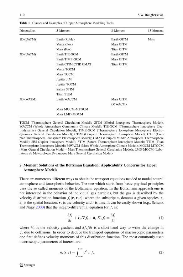
This chapter describes various numerical model classes (and representative model tools) thatare typically used in simulations of the upper atmospheres and ionospheres of planets. As-sumptions about the model equations to be solved by the different model frameworks can beclassified by the number of moments carried in the solution of the Boltzmann equation (seeTable 1 and Sect. 2). Both 1D and multi-dimensional model frameworks are employed, bothfor the upper atmosphere (UATM) and whole atmosphere (WATM) environment (see Ta-ble 1). One-dimensional models (see Sect. 3) are commonly used to thoroughly test detailedaeronomic processes (e.g., thermal, diffusion, and chemical) before the addition of globalwinds in a multi-dimensional model framework (see Sect. 4). This progression from 1D tomulti-dimensional models follows a development strategy involving increasing complexity,internal self-consistency, and expanded temporal plus spatial coverage. Finally, modelingfrontiers and key problems for further research are described in Sect. 5.
110 S.W. Bougher et al.
Table 1 Classes and Examples of Upper Atmosphere Modeling Tools
Dimensions 5-Moment 8-Moment 13-Moment
1D (UATM) Earth (Roble) Earth GITM Mars
Venus (Fox) Mars GITM
Mars (Fox) Titan GITM
3D (UATM) Earth TIE-GCM Earth GITM
Earth TIME-GCM Mars GITM
Earth CTIM,CTIP, CMAT Titan GITM
Venus TGCM
Mars TGCM
Jupiter JIM
Jupiter TGCM
Saturn STIM
Titan TTIM
3D (WATM) Earth WACCM Mars GITM
(MWACM)
Mars MGCM-MTGCM
Mars LMD-MGCM
TGCM (Thermosphere General Circulation Model); GITM (Global Ionosphere Thermosphere Model);WACCM (Whole Atmosphere Community Climate Model); TIE-GCM (Thermosphere Ionosphere Elec-trodynamics General Circulation Model); TIME-GCM (Thermosphere Ionosphere Mesosphere Electro-dynamics General Circulation Model); CTIM (Coupled Thermosphere Ionosphere Model); CTIP (Cou-pled Thermosphere Ionosphere Plasmasphere Model); CMAT (Coupled Middle Atmosphere ThermosphereModel); JIM (Jupiter Ionosphere Model); STIM (Saturn Thermosphere Ionosphere Model); TTIM (TitanThermosphere Ionosphere Model); MWACM (Mars Whole Atmosphere Climate Model); MGCM-MTGCM(Mars General Circulation Model – Mars Thermosphere General Circulation Model); LMD-MGCM (Labo-ratoire de Meteorologie Dynamique Mars General Circulation Model)
2 Moment Solutions of the Boltzman Equation: Applicability Concerns for UpperAtmosphere Models
There are numerous different ways to obtain the transport equations needed to model neutralatmosphere and ionospheric behavior. The one which starts from basic physical principlesuses the so called moments of the Boltzmann equation. In the Boltzmann approach one isnot interested in the behavior of individual gas particles, but the gas is described by thevelocity distribution function fs(r,v, t), where the subscript s, denotes a given species, s,rs is the spatial location, vs is the velocity and t is time. It can be easily shown (e.g., Schunkand Nagy 2000) that the integro-differential equation for fs is:
∂fs
∂t+ vs .∇fs + as .∇vfs = δfs
δt(1)
where ∇s is the velocity gradient and δfs/δt is a short hand way to write the change infs due to collisions. In order to deduce the transport equations of macroscopic parametersone first defines velocity moments of this distribution function. The most commonly usedmacroscopic parameters of interest are:
ns(r, t) =∫ ∞
−∞d3vsfs, (2)
Upper Atmosphere–Ionosphere Modeling 111
us(r, t) =∫ ∞
−∞d3vsfsvs/ns, (3)
Ts = ms
3kns
d3vsfs(vs − us)2, (4)
qs = ms
2
∫ ∞
−∞d3vsfs(vs − us)
2(vs − us), (5)
ps = ms
3
∫ ∞
−∞d3vsfs(vs − us)
2, (6)
Ps = ms
∫ ∞
−∞d3vsfs(vs − us)(vs − us), (7)
τs = Ps − psI, (8)
where ns is the number density of species s, us is the drift (mean) velocity, Ts is the temper-ature, qs is the heat flow vector, ps is the scalar pressure, Ps is the pressure tensor and τs isthe stress tensor.
In order to obtain the appropriate transport equations for these macroscopic parametersof interest one multiplies the Boltzmann equation with the appropriate function of velocityand then integrates over all velocities. Now a very important point should be noted thatthe resulting, so called “transport equations”, do not lead to a closed system of equations.Namely an equation governing the moment of order k contains the moment of order (k +1).As an example the equation for density contains the drift velocity. A number of approacheshave been suggested in order to achieve closure. The most commonly used method finds anapproximate expression for the distribution function which allows closure and the evaluationof the collision term.
The so-called 13 moment approximation is the most complex set of equations that havebeen used so far in neutral atmosphere and ionosphere modeling. In this approach, fs isapproximated as a truncated expansion about the Maxwell Boltzmann distribution functionin terms of density, drift velocity, temperature, stress tensor and heat flow vector. The name13-moment approximation comes from the fact that the gas is described in terms of 13 pa-rameters (ns = 1,us = 3, Ts = 1,qs = 3, τs = 5). In most cases the 13 moment equations(see Schunk and Nagy 2000) are too complicated to be able to be solved in a comprehensiveglobal model. The 8-moment equation neglects the stress tensor and the 5 moment equa-tions neglect both stress and heat flow. The Navier-Stokes equation are obtained from the13-moment equations by assuming that the collision frequency is very high and droppingall qs and τ s terms, except those that are multiplied by the collision frequency. In this ap-proximation qs and τ s can be expressed in term of ns , us and Ts . The most common set ofequations used in global models are these Navier-Stokes ones. However, it should be remem-bered that in this approximation the distribution function must be close to a Maxwellian.
3 Representative 1-D Neutral and/or Ion Models
3.1 Earth
A global mean model of a planetary atmosphere is useful for the development of a self-consistent aeronomical scheme, determining the vertical resolution necessary to determinethe basic atmospheric and ionospheric structure, time constants of physical and chemical
112 S.W. Bougher et al.
processes and a host of other properties of the atmosphere and ionosphere. Such a modelis numerically fast for long-time integrations, and easy to test and analyze the sensitivityof the atmosphere to physical and chemical processes, such as eddy diffusion, chemicalreactions, branching ratios, radiation to space and many other parameters. One can easilyconduct a large number of numerical simulations to develop an understanding of the impor-tant processes responsible for atmospheric structure and thus make it easier to transfer theimportant processes to other higher dimensional models.
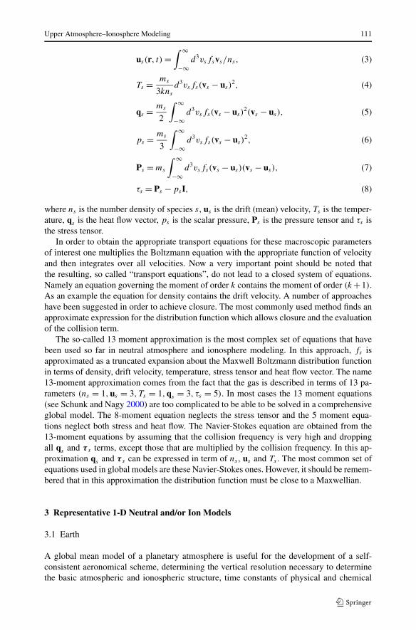
A 1D model that was important for the development of the series of National Centerfor Atmospheric Research (NCAR) TGCMs was developed by Roble et al. (1987) for thethermosphere and ionosphere. It was further extended to include the mesosphere and upperstratosphere by Roble (1995). A thorough description of the model has been given in the1995 paper. The model was designed to be fully consistent internally with only specificationof temperature and composition at the lower boundary at 10 mb (30 km) and the upperboundary in thermal and diffusive equilibrium (500–700 km). It is a time dependent modelgenerally run to steady state for global average forcing from solar EUV radiation, the aurora,and specified eddy diffusion. It was primarily used to develop the aeronomical scheme forthe series of TGCMs and to test ideas and parameters. It has been used for numerous studiesby colleagues and students to test various ideas. One example of a simulation for solarmedium conditions is shown in Fig. 1.
This terrestrial 1D code has also been used to study global change in the upper at-mosphere by Roble and Dickinson (1989) and more recently been used by Qian et al. (2006,2008) to study decadal changes in satellite drag and ionospheric structure.
3.2 Venus and Mars
One-dimensional models have been constructed of the thermospheres and ionospheres ofMars and Venus since the first radio occultation measurements of the electron density pro-files were reported from early flybys and orbiters. Lodders and Fegley (1998) have reviewedmissions to these planets up to 1998.
There are two basic types of one-dimensional models: photochemical equilibrium (PCE)models, in which transport is ignored, and those that include (usually) vertical transport ofspecies. While in the former type of model, the densities at each altitude can be computedindependently, in the latter type of model numerical coupling of each altitude to those aboveand below it must be taken into account. Altitude profiles of neutral species in thermospherescannot be modeled with the PCE approximation, although ion density profiles in the highdensity lower peak regions may be.
All of the early (and most of the subsequent) radio occultation electron density pro-files measured by radio science experiments of both Mars and Venus have exhibited twopeaks: an upper F1 peak, which is produced by absorption of the main portion of the EUV(∼150–1000 Å), and a lower E peak which is produced by the absorption of soft X-rays(e.g., Kliore et al. 1967; Stewart 1971). Curiously, however, the ion density profiles derivedfrom the Viking RPA measurements showed no lower peak (e.g., Hanson et al. 1977).
Most of the early models of the ionospheres of Mars and Venus that were designed to fitradio occultation electron density profiles, assumed PCE (e.g., McElroy 1967, 1968a, 1969;Stewart 1968, 1971). The Venus ionospheric model of Kumar and Hunten (1974), how-ever, was a hybrid model, in which the heavy ions were assumed to be in PCE, while thelighter ions were subject to transport. Shimazaki and Shimizu (1970) constructed a numberof models of the Martian ionosphere that included transport by diffusion and eddy diffusion,which were compared to the electron density profile measured by Mariner 4. Interestingly,
Upper Atmosphere–Ionosphere Modeling 113
Fig. 1 NCAR 1D global mean model simulations for solar medium conditions. (a) Neutral, ion, and electrontemperatures (∼30–400 km); (b) Neutral temperatures (40–120 km); (c) Heating terms of thermal equation(∼30–400 km); and (d) Cooling terms of the thermal equation (∼30–400 km). Individual curves for (a): Tn,Te, Ti: neutral, electron and ion temperatures; Tns : neutral temperature from MSIS-90. Individual curvesfor (c): SRC: Schumann-Runge Continuum; SRB: Schumann-Runge Bands; QT : total heating; QJ : Jouleheating; QA: auroral heating; O3: O3 heating; O(1D): heating from O(1D) quenching; QNC : neutral chem-istry heating; QIC : ion chemistry heating; QEI : ion–electron heating. Individual curves for (d): QT : totalheating; Ke : cooling rates from eddy thermal conduction; CO2: 15-micron cooling; NO: 5.3-micron cool-ing; Km: cooling rate from downward molecular thermal conduction; O(3P): oxygen fine structure cooling.ZP (left vertical axis, log pressure scale used by the NCAR codes)
McElroy (1968b) noted the difficulty of constructing model ionospheres when the only in-formation was in the form of radio occultation electron density profiles, without the benefitof in situ measurements of ion and neutral densities. The lack of in situ measurements hasalso plagued interpretation of the electron density profiles of the outer planets for manyyears.
The PCE approximation becomes inaccurate above the boundary where the lifetime of aspecies due to chemistry (τc = 1/L), where L = L/n is the specific loss rate, L is the totalchemical loss rate and n is the number density of the species, becomes longer than that due tovertical transport. If the main transport process is by diffusion, the lifetime of a species due totransport is given approximately as τD ∼ H 2/D, where D is the diffusion coefficient of thatspecies and H = kT /mg is the scale height. In this expression, k is Boltzmann’s constant,while T ,g, and m are the altitude dependent temperature, acceleration of gravity, the mass
114 S.W. Bougher et al.
of the atmospheric species, respectively. For ions, the scale height is Hi = k(Ti + Te)/mig,where Ti is the ion temperature, and Te is the electron temperature.
If the major transport process (for neutrals) is mixing, the lifetime of a species againsttransport is given by τK ∼ H 2
avg/K , where K is the eddy diffusion coefficient, Havg =kT /mavgg, and mavg is the average mass of the constituents. It is remarkable that the eddydiffusion coefficient is on the order of 1.0 × 10¹³/n0.5 cm2 s−1, where n is the total num-ber density in the lower thermospheres for both Mars and Venus (cf., Krasnopolsky 1982;von Zahn et al. 1980).
The boundary where diffusion of a neutral species becomes more important than mix-ing is known as the homopause. In fact, however, that altitude is different for each species.In early models of the thermospheres of Venus and Mars, a single homopause altitude wasassumed (e.g., McElroy 1967, 1969; Kumar and Hunten 1974; Chen and Nagy 1978). Be-low the homopause the thermosphere is considered to be completely mixed for chemicaltracers/inert species; above the homopause, these species density profiles are assumed to bedistributed according to their own scale heights. Species that are formed photochemically donot exhibit this behavior. Because of the availability of in situ measurements of the neutraldensities, and the computing power that is available today, even in one-dimensional models,the homopause approximation is neither necessary nor used widely.
While PCE approximations are almost never used to compute the density profiles ofminor neutral thermospheric species, such models of ion density profiles continue to beused for specific purposes, including studies focused on the electron density peak regions(e.g., Cravens et al. 1981; Fox and Dalgarno 1981; Kim et al. 1989; Martinis et al. 2003), orfor airglow calculations of processes that originate near the electron density peaks (see, forexample Fox 1992, and references therein).
The Viking I and II probes carried neutral mass spectrometers through the Martianatmosphere, and so the major neutral densities in the thermosphere at low solar ac-tivity were measured in situ for the first time (e.g., Nier and McElroy 1976). Earlyionospheric models based on these measurements included, for example, those of McEl-roy et al. (1976), Fox and Dalgarno (1979), and Chen et al. (1978). While the lattermodel included vertical transport. The former two were photochemical equilibrium mod-els. The in situ measurements of the Pioneer Venus orbiter and probes enabled more ac-curate models of the Venusian ionosphere (e.g., Chen and Nagy 1978; Nagy et al. 1980;Fox 1982).
In the terrestrial ionosphere, the absolute maximum in the electron density profile is anF2 peak, which appears near 300 km. At this altitude, the chemical lifetime of the major ion(O+) is approximately equal to that of transport. At high altitudes in the Venus ionosphere,O+ becomes the most important species, yet models show that it forms a peak that is not(or is barely) visible in the electron density profile. On Mars, the O+ density forms a peakat high altitudes, but thus far measurements indicate that densities of O+ are everywheresmaller than those of O+
2 (e.g., Hanson et al. 1977). Where the major loss is by transport,photochemical equilibrium models do not reproduce the profiles of ions, such as O+ andother (mostly) atomic ions.
More sophisticated one-dimensional thermosphere/ionosphere models have includedboth chemistry and transport by molecular and eddy diffusion (for neutrals), and ambipo-lar diffusion (for ions), and do not assume a fixed homopause (e.g., Nagy et al. 1980; Fox1982, 2004; Krasnopolsky 2002). The one-dimensional thermosphere-ionosphere models ofVenus and Mars of Shinagawa and Cravens (1988, 1989) have also included magnetic fields.
Although one-dimensional models have limitations, mainly that horizontal transport byconvection is ignored, they are simple enough that many species and reactions among those
Upper Atmosphere–Ionosphere Modeling 115
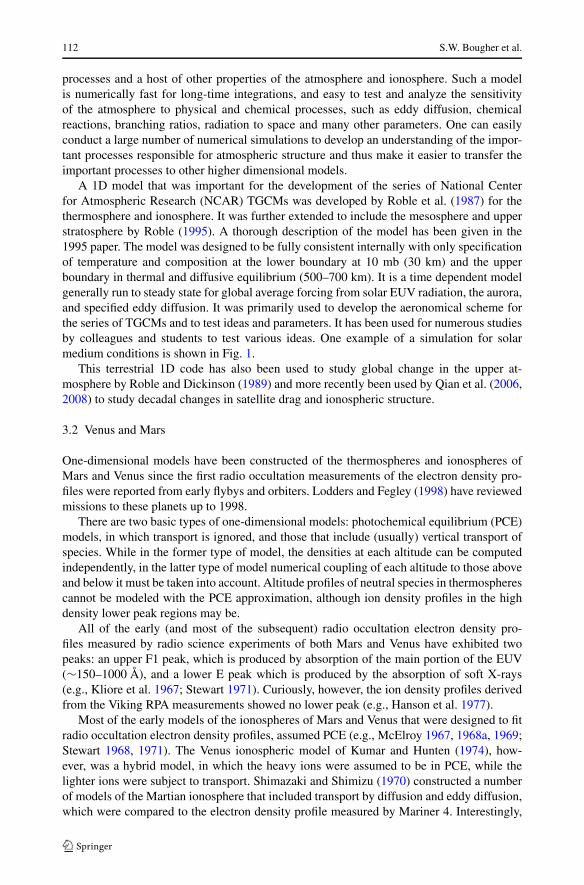
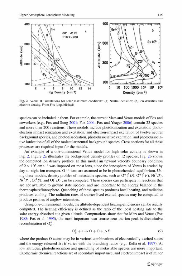
Fig. 2 Venus 1D simulations for solar maximum conditions: (a) Neutral densities; (b) ion densities andelectron density. From Fox (unpublished)
species can be included in them. For example, the current Mars and Venus models of Fox andcoworkers (e.g., Fox and Sung 2001; Fox 2004; Fox and Yeager 2006) contain 23 speciesand more than 200 reactions. These models include photoionization and excitation, photo-electron impact ionization and excitation, and electron-impact excitation of twelve neutralbackground species, and photodissociation, photodissociative excitation, and photodissocia-tive ionization of all of the molecular neutral background species. Cross sections for all theseprocesses are required input for the models.
An example of a one-dimensional Venus model for high solar activity is shown inFig. 2. Figure 2a illustrates the background density profiles of 12 species; Fig. 2b showsthe computed ion density profiles. In this model an upward velocity boundary conditionof 2 × 105 cm s−1 was imposed on most ions, since the ionosphere of Venus is eroded byday-to-night ion transport. O++ ions are assumed to be in photochemical equilibrium. Us-ing these models, density profiles of metastable species, such as O+(2D), O+(2P ), N(2D),N(2P ), O(1S), and O(1D) can be computed. These species can participate in reactions thatare not available to ground state species, and are important to the energy balance in thethermosphere/ionosphere. Quenching of these species produces local heating, and radiationproduces cooling. The radiation rates of shorter-lived excited species may be computed toproduce profiles of airglow intensities.
Using one-dimensional models, the altitude-dependent heating efficiencies can be readilycomputed. The heating efficiency is defined as the ratio of the local heating rate to thesolar energy absorbed at a given altitude. Computations show that for Mars and Venus (Fox1988; Fox et al. 1995), the most important heat source near the ion peak is dissociativerecombination of O+
2 ,
O+2 + e → O + O + �E (9)
where the product O atoms may be in various combinations of electronically excited statesand the energy released �/E varies with the branching ratios (e.g., Kella et al. 1997). Atlow altitudes, photodissociation and quenching of metastable species are more important.Exothermic chemical reactions are of secondary importance, and electron impact is of minor
116 S.W. Bougher et al.
importance over the entire thermosphere. For Venus, the altitude dependent heating efficien-cies range from about 16% at low altitudes for the “lower limit” model to 22% for the “bestguess” model. At high altitudes the heating efficiencies increase slightly with altitude up to185 km. On Mars, the “best guess model” yields heating efficiencies of about 21 ± 2% from100 to 200 km, although at low altitudes the lower limit model shows heating efficiencies ofabout 16%.
4 Representative Multidimensional Models
4.1 Model Classes to be Addressed
Table 1 summarizes the classes of multi-dimensional models that we will consider inSects. 4 and 5. Notice that multi-dimensional model development is following two im-portant trends. First, existing upper atmosphere models are being extended to encom-pass the entire atmosphere domain (ground to exosphere) for Earth (NCAR WACCM)and Mars (Michigan-MWACM). The LMD-MGCM code for the Mars lower atmospherehas also be extended upward into the thermosphere. These efforts reflect the availabil-ity of both lower and upper atmosphere datasets for these planets. Coupling processes(thermal, chemical, dynamical) linking these atmospheric regions are important to ad-dress with these “whole atmosphere” modeling tools. Second, model frameworks are be-ing developed and exercised using 8-moment and 13-moment solutions of the Boltzmanequation. The motivations here are at least twofold: (a) to incorporate a non-hydrostatictreatment for improvement of the simulation of vertical velocities (Ridley et al. 2006;Deng et al. 2008), and (b) to capture the physical processes that bridge the collisional andnon-collisional regions near the exobase (Boqueho and Blelly 2005).
Under hydrostatic equilibrium, a typical assumption used in most global planetary mod-els, the pressure gradient in the vertical direction is exactly balanced by the gravity force(Deng et al. 2008). However, for large vertical velocities, acceleration terms in the verticalmomentum equation cannot be ignored, and the basic balance is no longer hydrostatic. Twolikely examples of these conditions are realized for the sudden intense enhancement of highlatitude Joule heating for the Earth’s thermosphere-ionosphere (Deng et al. 2008), and thatof Jupiter as well. If the hydrostatic assumption is relaxed, the vertical momentum equa-tion can be expanded to include additional acceleration terms: (1) forces due to ion-neutraland neutral-neutral friction (when each constituent is solved independently), (2) centrifugaland Coriolis forces, and (3) non-linear advection terms. The altitude variation of gravityis easily accommodated in this framework. Vertical propagation of a non-hydrostatic “dis-turbance” results in acoustic waves and non-hydrostatic gravity waves (Deng et al. 2008).Care must be taken to either damp or accommodate these waves in non-hydrostatic mod-els. In short, global non-hydrostatic models are needed to address phenomenon associ-ated with large vertical winds in planetary upper atmospheres. New planet specific globalthermosphere–ionosphere models are being developed and validated for this purpose, basedupon the Global Thermosphere–Ionosphere Model (GITM) for Earth (Ridley et al. 2006;Deng et al. 2008).
4.2 Representative GCM Model Descriptions/Results
4.2.1 Earth (NCAR TGCMs)
A series of TGCMs have been developed at NCAR over the past 30 years with each modelincorporating new processes of the coupled thermosphere-ionosphere system. The histori-
Upper Atmosphere–Ionosphere Modeling 117
cal development of the TGCM suite of models is discussed in Bougher et al. (2002). Self-consistent temperatures, neutral-ion densities, neutral dynamics, and self-consistent electro-dynamics are contained in the TIE-GCM (Richmond et al. 1992). This code was then ex-tended to include the mesosphere and upper stratosphere to become the TIME-GCM (Robleand Ridley 1994). These two codes are now the basic upper atmosphere models at NCAR.The TIE-GCM is used to explore thermosphere-ionosphere-electrodynamic interactions andthe TIME-GCM has the same processes but extended to include aeronomic processes asso-ciated with the mesosphere and upper stratosphere and to examine physical and chemicalinteractions between upper atmospheric regions.
The TIME-GCM is a self-consistent model of the upper atmosphere extending between30 km and 500 km altitude. It has been used for comparison and interpretation of satellite,rocket and ground-based data for many years by a wide variety of scientific colleagues,post doctoral fellows and graduate students. The TIME-GCM was initially designed for a5◦ latitude and longitude grid in the horizontal and 2 grid points per scale height in thevertical with a 5 minute time step. This “coarse” horizontal and vertical resolution waslater refined for specific model applications (see below). The TIME-GCM solves for theneutral gas temperature, winds and constituents of the thermosphere, mesosphere and upperstratosphere both major and minor species self-consistently. It also solves for the ionosphericplasma properties of electron and ion temperature, electron density and ion composition,and the electric field, plasma drift and resulting magnetic perturbations. The most recentdescription of the model is given by Roble (2000).
In the late 1990s, the TIME-GCM was extended to use lower boundary data at 10 mb(30 km) to force the variability propagating upward from the lower atmosphere and to studycouplings between the lower and upper atmospheres (Roble 2000). This included specifica-tion of tides, gravity waves, planetary waves and other disturbances on a daily basis so thatcontinuous simulations of the upper atmosphere could be made for realistic daily simula-tions that would be used to compare with observational time averaged campaign or satelliteorbital tracking data.
In order to examine the feasibility of developing a model that extended from the ground-to-exosphere the TIME-GCM was flux coupled to the NCAR community climate modelCCM3 (Khiel et al. 1998) at the boundary between the models near 10 mb. This allowed in-formation between the upper and lower atmospheres to be exchanged simulating the entireatmosphere, troposphere, stratosphere, mesosphere and thermosphere/ionosphere. This cou-pled model simulated a strong stratospheric warming, mesospheric cooling, thermosphericwarming at high latitudes that was generated spontaneously from planetary waves propagat-ing upward from the troposphere (Liu and Roble 2002, 2005). These studies indicated thata continuous model from the ground to exosphere could be developed to examine couplingaspects between regions of the whole atmosphere. This was a precursor for the developmentof the WACCM that is discussed in Sect. 5.1.2.
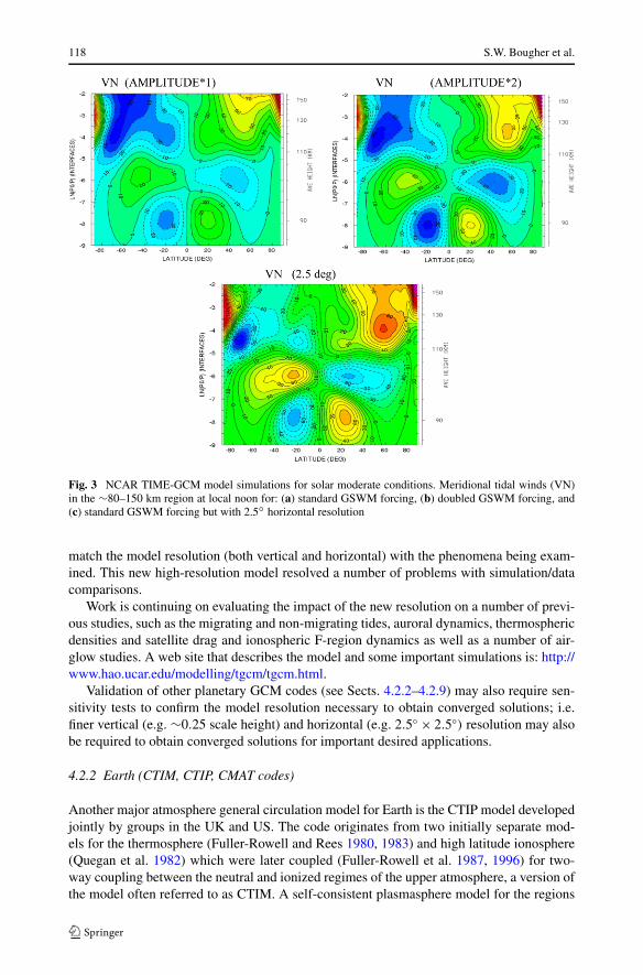
The TIME-GCM resolution was limited by computer power in the 1990s and early 2000s.While this was sufficient for a number of upper atmosphere studies, it was inadequate to rep-resent the shorter wave migrating and non-migrating tides and planetary wave propagationand dissipation. One temporary solution was to double the amplitudes of the Global ScaleWave Model (GSWM) forcing at the lower boundary to get agreement with observationaldata. Subsequent simulations showed that it was not necessary to double the amplitudes butrather to improve both the vertical (0.25 scale height) and horizontal (2.5◦ × 2.5◦) resolu-tion. These comparisons are shown in Fig. 3. With a double resolution, large tides developedwithout the need to double GSWM amplitudes. This exercise clearly illustrates the need to
118 S.W. Bougher et al.
Fig. 3 NCAR TIME-GCM model simulations for solar moderate conditions. Meridional tidal winds (VN)in the ∼80–150 km region at local noon for: (a) standard GSWM forcing, (b) doubled GSWM forcing, and(c) standard GSWM forcing but with 2.5◦ horizontal resolution
match the model resolution (both vertical and horizontal) with the phenomena being exam-ined. This new high-resolution model resolved a number of problems with simulation/datacomparisons.
Work is continuing on evaluating the impact of the new resolution on a number of previ-ous studies, such as the migrating and non-migrating tides, auroral dynamics, thermosphericdensities and satellite drag and ionospheric F-region dynamics as well as a number of air-glow studies. A web site that describes the model and some important simulations is: http://www.hao.ucar.edu/modelling/tgcm/tgcm.html.
Validation of other planetary GCM codes (see Sects. 4.2.2–4.2.9) may also require sen-sitivity tests to confirm the model resolution necessary to obtain converged solutions; i.e.finer vertical (e.g. ∼0.25 scale height) and horizontal (e.g. 2.5◦ × 2.5◦) resolution may alsobe required to obtain converged solutions for important desired applications.
4.2.2 Earth (CTIM, CTIP, CMAT codes)
Another major atmosphere general circulation model for Earth is the CTIP model developedjointly by groups in the UK and US. The code originates from two initially separate mod-els for the thermosphere (Fuller-Rowell and Rees 1980, 1983) and high latitude ionosphere(Quegan et al. 1982) which were later coupled (Fuller-Rowell et al. 1987, 1996) for two-way coupling between the neutral and ionized regimes of the upper atmosphere, a version ofthe model often referred to as CTIM. A self-consistent plasmasphere model for the regions
Upper Atmosphere–Ionosphere Modeling 119
equatorward of around 30◦ geomagnetic latitude was added by Millward et al. (1996a) toform CTIP. More recently, the original bottom boundary (80 km, 0.01 mb) of the CTIMmodel was lowered by Harris (2001) into the stratosphere (30 km, 10 mb) in order to in-clude the stratospheric and mesospheric chemistry and full vertical dynamical and chemicalcoupling. This extended version of the model is referred to as the CMAT model.
What distinguishes these from other thermosphere/ionosphere models is primarily thefact that ionospheric calculations are carried out along magnetic field lines rather than be-ing treated on the same spherical grid as the neutral gases. This has proven to be a mostuseful approach since one key issue is how to treat upper boundary conditions for ions andelectrons, in particular the plasma fluxes along field lines in the topside ionosphere wherefield-aligned transport forms a dominant process affecting the distribution of O+ and H+ions and electrons. The plasma flux boundary condition becomes important for calculationsof ionospheric densities when the boundary is located within a few scale heights above thedensity peak. The particular choice of flux tube coordinates for plasma in CTIP/CTIM elim-inates this difficulty. At high latitudes field lines are open and extend to around 10000 kmaltitude in the model, while at low latitudes flux tubes in CTIP are closed. With plasmadensities near 10000 km being negligible compared with ionospheric densities, a zero fluxboundary condition can safely be assumed, while in the regime of closed flux tubes bothends of a field line are within the photochemical domain of the ionosphere (in oppositehemispheres), allowing the simple boundary condition of photochemical equilibrium.
The CTIP, CTIM and CMAT models have been used extensively over the past decadesto understand the global morphology of the thermosphere and ionosphere both throughpurely theoretical studies and in comparisons with observations. Studies have investigated(amongst others) the morphology of responses to geomagnetic storms (Field et al. 1998;Fuller-Rowell et al. 2002), thermospheric composition and dynamics (Fuller-Rowell 1998;Rishbeth and Mueller-Wodarg 1999), semiannual variations in the ionosphere (Millwardet al. 1996b; Rishbeth et al. 2000a), effects of tidal forcing (Millward et al. 2001;Mueller-Wodarg et al. 2003) and NO chemistry (Dobbin et al. 2006).
4.2.3 Michigan GITM Codes
Earth GITM. The GITM code (Ridley et al. 2006) was designed from the bottom up withflexibility in mind for every aspect of modeling upper atmospheres of planetary systems.The grid system within GITM is fully parallel and is quite versatile. Users can run 1D casesat a specified latitude and longitude (which is set at run-time in the input file) or 3D caseswith almost any latitudinal and longitudinal resolution that the user wants (once again, set atrun-time). GITM can run on a single processor machine or multi-processor machines. It hasbeen run on 256 processors resolving the upper atmosphere with a 1.25◦ latitudinal by 2.5◦longitudinal resolution. For testing, GITM has been run with 10◦ by 20◦ resolution. Thisflexibility in the resolution allows rapid development of the model and facilitates testing ofnew physics within the code.
The main feature that differentiates GITM from all other coupled ionosphere ther-mosphere models is the easing of the hydrostatic assumption within the vertical momentumequation—the pressure does not have to balance with gravity (although it almost alwaysdoes). In regions in which there are non-hydrostatic forces (e.g., the auroral zone), largevertical winds can develop (Deng et al. 2008). In addition, the GITM vertical momentumequation allows gravity to be dependent on altitude, instead of constant, which is crucialfor small bodies with extended atmospheres, such as Titan. GITM utilizes an altitude grid,which is also different than other upper atmosphere models. The resolution in the verticaldirection is stretched such that it is approximately 1/3 of a scale height at code initiation.
120 S.W. Bougher et al.
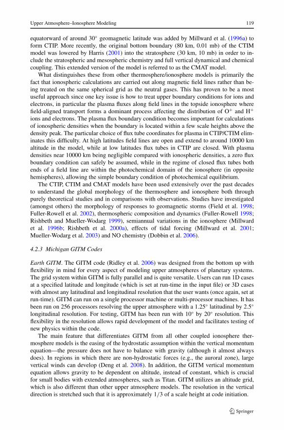
Fig. 4 Earth GITM simulation at 400 km. Horizontal wind vectors are superimposed upon mass densitycolor contours (1.15 to 5.15 × 10⁻¹² g/m3)
An additional feature of GITM is the ability to turn on and off physics through the inputfile. Different source terms (such as Coriolis, Joule heating, solar EUV heating, and thermalconduction), can be turned off through the input file. This allows users to conduct numericalexperiments in which they self-consistently determine the effects of different source termson the coupled nonlinear system.
In order to allow GITM to be utilized for more than a single body, very little was hard-coded into the core of GITM. Each atmospheric and ionospheric constituent is specified ina planet specific module, such that the advective core need only loop over the number ofspecies to determine the hydrodynamic behavior of the atmosphere. Other common sourceterms, such as solar EUV inputs, and inter-species frictional drag in the vertical direction, arehandled in a similar manner, allowing the code to be adapted to another planet very easily.More specific source terms, such as radiative cooling, need to be coded for the particularproblem and are easily linked to GITM through hooks.
At Earth, GITM has an extremely flexible high-latitude energy input module. This al-lows users to try different electric fields and particle inputs to drive GITM. At other planets,this can be easily adapted to different types of forcing. Models of electron precipitation andelectric potential can be added with little difficulty. These will then be utilized to calcu-late electric fields and ion and electron velocities. Joule heating and ion-neutral momentumcoupling are then self-consistently calculated.
Figure 4 shows results from the Earth-based GITM at 400 km altitude. The vectors showthe thermospheric neutral winds, while the coloring is the thermospheric mass density. Theneutral winds roughly follow a two-cell convection pattern at high latitudes, due to the strongforcing by the ion convection and aurora. On the dusk-side (left), the neutrals are able toform a completely closed cell, while on the dawn-side (right), the cell is less well defined.
Upper Atmosphere–Ionosphere Modeling 121
This is because on the dusk-side, the Coriolis force is in the same direction as the circulationpattern, so the closed cell is accentuated, while on the dawn-side, the flow is inhibited, sincethe Coriolis force opposes it. At very high latitudes and at the tail end of the convection cellson the night side (i.e., just over Canada), there is a large enhancement in the thermosphericmass density. This is caused by Joule heating in the auroral zone, where there are extremelylarge electric fields and strong conductivities. During this strong driving period, the densitypeaks at the poles, while during quieter times, the mass density peaks at lower latitudes.
Titan GITM. A new application of the GITM framework was recently developed (Bell etal. 2006; Bell 2008) in an effort to interpret and place in a global context new Cassini INMSneutral and ion density and inferred temperature datasets of the Titan upper atmosphere(e.g., Waite et al. 2005). The GITM framework was chosen to capture the unique physics ofthe Titan upper atmosphere that requires: (a) variable gravity, (b) calculated fluxes of ma-jor species out the top of the atmosphere, and (c) variable Saturn magnetospheric forcing.Density gradients (yielding fluxes) were specified at the upper boundary in order to sim-ulate measured Cassini INMS CH4 density profiles; the self-consistent feedback of thesefluxes upon temperatures was also included. The Titan GITM code was designed to span∼500 to 1500 km in the Titan upper atmosphere, covering the region below the homopause(∼800 km) to just above the exobase (∼1300 km). Solar EUV forcing (heating, photo-dissociation, photo-ionization) is dominated by N2 and CH4 solar absorption between 1.6–170.0 nm. Hydrogen cyanide (HCN) rotational band infrared radiative cooling is incorpo-rated and represents the dominant IR cooling agent in the thermosphere. A self-consistenttreatment of chemical production and loss processes for 4-major, 7-minor, several isotopes,and thermally active (e.g. HCN) constituents is incorporated, based upon the scheme out-lined by DeLa Haye (2005). Major photochemical ions are limited to key species: N+
2 , N+,CH+
3 , H2CN+, and C2H+5 . Finally, a differentially, super-rotating lower boundary is specified
at ∼500 km, in accord with ground-based observations (Hubbard et al. 1993). Horizontaland vertical distributions of simulated temperatures and densities have been successfullycompared to specific Cassini orbit measurements, especially profiles of key isotopes (e.g.,Bell 2008).
Mars GITM. The need for a ground-to-exobase GCM at Mars has motivated another newapplication of the GITM framework. Existing Mars lower and upper atmosphere datasetsneed to be interpreted and connected using such a “whole atmosphere” model framework(e.g., Bougher et al. 2006b). This is the first extension of the GITM framework over a widerange of altitudes encompassing both upper and lower atmosphere processes.
A prototype MWACM code using the GITM framework has been developed, enablinginitial 1D and 3D simulations to be conducted over 0–300 km for specific solar cycle, sea-sonal and dust conditions at Mars. Specifically, the terrestrial GITM code (Ridley et al. 2006)was adapted to include Mars fundamental parameters, constants, and key radiative processesin order to capture the basic observed features of the thermal and dynamical structure of theMars atmosphere from the ground to 300 km. For the Mars lower atmosphere (0–80 km),an efficient (fast) radiation code was adapted from the NASA Ames MGCM code to theframework of the MWACM. This now provides MWACM solar heating (long and shortwavelength), aerosol heating, and CO2 15-micron cooling in the LTE region of the Marsatmosphere below ∼80 km. For the Mars upper atmosphere (∼80 to 300 km), a fast formu-lation for NLTE CO2 15-micron cooling was implemented into the MWACM code, alongwith a correction for non-LTE (NLTE) near-IR heating rates (∼80–120 km). In addition,a thermospheric EUV-UV heating routine (based upon a CO2 dominated atmosphere) wasadapted to the MWACM framework. Finally, detailed neutral-ion chemistry was recentlyincorporated above 80 km, based upon Mars TGCM reactions and rates (see Sect. 4.2.5).
122 S.W. Bougher et al.
For the entire atmosphere, the MWACM dynamical core solver was modified to workwith the new terrain following coordinate system. The Martian terrain is now being incor-porated into the MWACM code making use of Mars Global Surveyor MOLA topographicdata files. NASA Ames MGCM CO2 condensation, and boundary layer routines will beadded below 80 km. At the surface, global empirical maps of albedo and thermal inertia willbe supplied to the radiation calculations. Initial simulations indicate this extended model isstable and captures the basic observed temperatures and expected wind structures through-out the Mars atmosphere.
4.2.4 Venus (NCAR VTGCM)
The large-scale circulation of the Venus upper atmosphere from ∼90 to ∼200 km (uppermesosphere and thermosphere) is a combination of two distinct flow patterns: (1) a rel-atively stable subsolar-to-antisolar (SS-AS) circulation cell driven by solar (EUV-UV-IR)heating, and (2) a highly variable retrograde superrotating zonal (RSZ) flow (see reviewsby Bougher et al. 1997, 2006a, 2006b; Schubert et al. 2007). GCMs have proven usefulfor synthesizing the available Pioneer Venus, Magellan, Venus Express, and ground-baseddensity, temperature, and/or airglow datasets and thereby extracting these upper atmospherewind components (see reviews by Bougher et al. 1997, 2006a; Schubert et al. 2007).
The Venus TGCM (VTGCM) is a 3D finite difference hydrodynamic model of the Venusupper atmosphere that is based on the NCAR terrestrial TGCM. The VTGCM has beendocumented in detail as revisions and improvements have been made over nearly 2-decades(see Bougher et al. 1988, 1990, 1997, 1999a, 2002; Bougher and Borucki 1994; Zhang et al.1996).
The modern VTGCM code (e.g., Brecht et al. 2007; Rafkin et al. 2007; Bougher etal. 2008) calculates global distributions of major species (CO2, CO, O, and N2), minorspecies (e.g. O2, NO, N(4S), N(2D)), and dayside photochemical ions (CO+
2 , O+2 , O+, and
NO+). These constituent fields are all consistent with the simulated 3-D temperature struc-ture and the corresponding 3-component neutral winds. The VTGCM model covers a 5◦by 5◦ latitude-longitude grid, with 46 evenly spaced log-pressure levels in the vertical, ex-tending from approximately ∼80 to 200 km at local noon. Dayside O and CO sources ariseprimarily from CO2 net dissociation and ion-neutral chemistry; the latter utilizes the ion-neutral chemical reactions and rates of Fox and Sung (2001). Simplified catalytic ClOx andHOx reactions can also employed to specifically improve the chemical sources and sinks forO and CO below 120 km (e.g., Bougher and Borucki 1994).
Formulations for CO2 15-micron cooling, wave drag, and eddy diffusion are incorporatedinto the VTGCM (see Bougher et al. 1999a; Brecht et al. 2007). In particular, CO2 15-micron emission is known to be enhanced by collisions with O atoms, providing increasedcooling in NLTE regions of the upper atmosphere (see Bougher et al. 1994; Kasprzak etal. 1997). VTGCM CO2 15-micron cooling is parameterized as described by Bougher et al.(1986), making use Roldan et al. (2000) exact cooling profiles at reference temperatures andatomic oxygen abundances. The collisional O–CO2 relaxation rate adopted for simulated15-micron cooling is ∼3 × 10⁻¹² cm3/s. In addition, near-IR heating rates are incorporatedusing modern offline look-up tables from Roldan et al. (2000). These parameterizationsprovide strong CO2 15-micron cooling that is consistent with the use of EUV-UV heatingefficiencies of ∼20–22%, which are in agreement with detailed offline heating efficiencycalculations of Fox (1988).
The VTGCM is typically run to examine Venus thermospheric structure and winds forsolar maximum, moderate, and minimum EUV-UV flux conditions, corresponding to terres-trial F10.7-cm indices of 200, 110-130, and 68-80, respectively. In addition, the VTGCM
Upper Atmosphere–Ionosphere Modeling 123
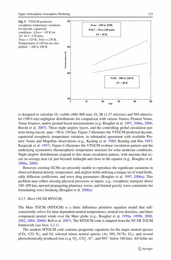
Fig. 5 VTGCM predictedexospheric temperature variationsfor dayside, equatorialconditions. �Texo ∼ 95 K for�F 10.7∼170 units.Tmax = 325 K; Tmin = 230 K.Temperatures at 140 km are alsoplotted: ∼200 to 240 K
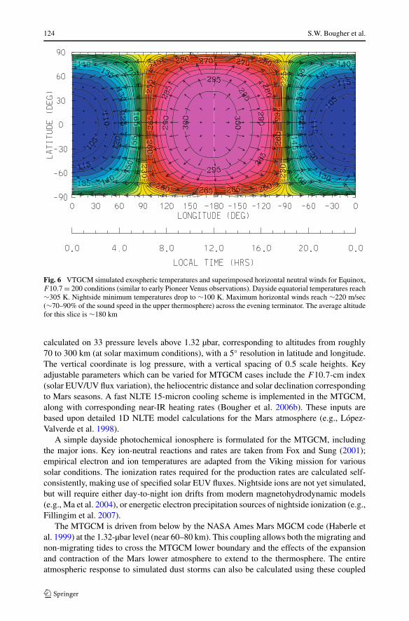
is designed to calculate O2 visible (400–800 nm), O2 IR (1.27 microns) and NO ultravio-let (198.0 nm) nightglow distributions for comparison with various Venera, Pioneer Venus,Venus Express, and/or ground-based measurements (e.g. Bougher et al. 1997, 2006a, 2008;Brecht et al. 2007). These night airglow layers, and the controlling global circulation pat-terns being traced, span ∼90 to 150 km. Figure 5 illustrates the VTGCM predicted dayside,equatorial exospheric temperature variation, in substantial agreement with available Pio-neer Venus and Magellan observations (e.g., Keating et al. 1980; Keating and Hsu 1993;Kasprzak et al. 1997). Figure 6 illustrates the VTGCM exobase circulation pattern and theunderlying asymmetric thermospheric temperature structure for solar moderate conditions.Night airglow distributions respond to this mean circulation pattern, with maxima that oc-cur on average near (or just beyond) midnight and close to the equator (e.g., Bougher et al.2006a, 2008).
However, existing GCMs are presently unable to reproduce the significant variations inobserved diurnal density, temperature, and airglow fields utilizing a unique set of wind fields,eddy diffusion coefficients, and wave drag parameters (Bougher et al. 1997, 2006a). Thisproblem may reflect missing physical processes or inputs, e.g., exospheric transport above180–200 km, upward propagating planetary waves, and limited gravity wave constraints forformulating wave breaking (Bougher et al. 2006a).
4.2.5 Mars (NCAR MTGCM)
The Mars TGCM (MTGCM) is a finite difference primitive equation model that self-consistently solves for time-dependent neutral temperatures, neutral-ion densities, and threecomponent neutral winds over the Mars globe (e.g., Bougher et al. 1999a, 1999b, 2000,2002, 2004, 2006b; Bell et al. 2007). The MTGCM code is adapted from the NCAR TGCMframework (see Sect. 4.2.1).
The modern MTGCM code contains prognostic equations for the major neutral species(CO2, CO, N2, and O), selected minor neutral species (Ar, NO, N(4S), O2), and severalphotochemically produced ions (e.g. O+
2 , CO+2 , O+, and NO+ below 180 km). All fields are
124 S.W. Bougher et al.
Fig. 6 VTGCM simulated exospheric temperatures and superimposed horizontal neutral winds for Equinox,F10.7 = 200 conditions (similar to early Pioneer Venus observations). Dayside equatorial temperatures reach∼305 K. Nightside minimum temperatures drop to ∼100 K. Maximum horizontal winds reach ∼220 m/sec(∼70–90% of the sound speed in the upper thermosphere) across the evening terminator. The average altitudefor this slice is ∼180 km
calculated on 33 pressure levels above 1.32 µbar, corresponding to altitudes from roughly70 to 300 km (at solar maximum conditions), with a 5◦ resolution in latitude and longitude.The vertical coordinate is log pressure, with a vertical spacing of 0.5 scale heights. Keyadjustable parameters which can be varied for MTGCM cases include the F10.7-cm index(solar EUV/UV flux variation), the heliocentric distance and solar declination correspondingto Mars seasons. A fast NLTE 15-micron cooling scheme is implemented in the MTGCM,along with corresponding near-IR heating rates (Bougher et al. 2006b). These inputs arebased upon detailed 1D NLTE model calculations for the Mars atmosphere (e.g., López-Valverde et al. 1998).
A simple dayside photochemical ionosphere is formulated for the MTGCM, includingthe major ions. Key ion-neutral reactions and rates are taken from Fox and Sung (2001);empirical electron and ion temperatures are adapted from the Viking mission for varioussolar conditions. The ionization rates required for the production rates are calculated self-consistently, making use of specified solar EUV fluxes. Nightside ions are not yet simulated,but will require either day-to-night ion drifts from modern magnetohydrodynamic models(e.g., Ma et al. 2004), or energetic electron precipitation sources of nightside ionization (e.g.,Fillingim et al. 2007).
The MTGCM is driven from below by the NASA Ames Mars MGCM code (Haberle etal. 1999) at the 1.32-µbar level (near 60–80 km). This coupling allows both the migrating andnon-migrating tides to cross the MTGCM lower boundary and the effects of the expansionand contraction of the Mars lower atmosphere to extend to the thermosphere. The entireatmospheric response to simulated dust storms can also be calculated using these coupled
Upper Atmosphere–Ionosphere Modeling 125
Fig. 7 MTGCM exospherictemperatures as a function of Ls
(season) and solar cycle(F10.7-cm index). Dayside(LT = 1500) equatorialconditions are displayed. Curvesindicated: F10.7 = 175–200(top), 110–130 (middle), and70–80 (bottom)
models. Key prognostic variables are passed upward from the MGCM to the MTGCM atthe 1.32-µbar level at every MTGCM grid point: temperatures, zonal and meridional winds,and geopotential heights. These two climate models are each run with a 2-minute time step,with the MGCM exchanging fields with the MTGCM at this frequency.
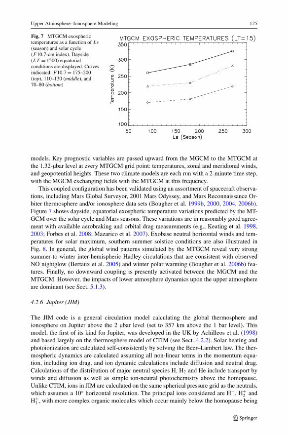
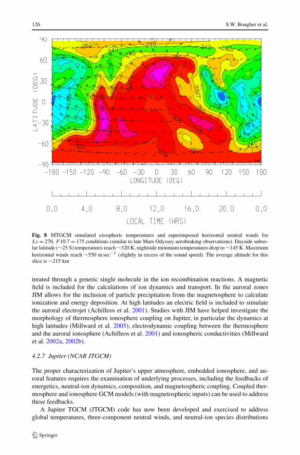
This coupled configuration has been validated using an assortment of spacecraft observa-tions, including Mars Global Surveyor, 2001 Mars Odyssey, and Mars Reconnaissance Or-biter thermosphere and/or ionosphere data sets (Bougher et al. 1999b, 2000, 2004, 2006b).Figure 7 shows dayside, equatorial exospheric temperature variations predicted by the MT-GCM over the solar cycle and Mars seasons. These variations are in reasonably good agree-ment with available aerobraking and orbital drag measurements (e.g., Keating et al. 1998,2003; Forbes et al. 2008; Mazarico et al. 2007). Exobase neutral horizontal winds and tem-peratures for solar maximum, southern summer solstice conditions are also illustrated inFig. 8. In general, the global wind patterns simulated by the MTGCM reveal very strongsummer-to-winter inter-hemispheric Hadley circulations that are consistent with observedNO nightglow (Bertaux et al. 2005) and winter polar warming (Bougher et al. 2006b) fea-tures. Finally, no downward coupling is presently activated between the MGCM and theMTGCM. However, the impacts of lower atmosphere dynamics upon the upper atmosphereare dominant (see Sect. 5.1.3).
4.2.6 Jupiter (JIM)
The JIM code is a general circulation model calculating the global thermosphere andionosphere on Jupiter above the 2 µbar level (set to 357 km above the 1 bar level). Thismodel, the first of its kind for Jupiter, was developed in the UK by Achilleos et al. (1998)and based largely on the thermosphere model of CTIM (see Sect. 4.2.2). Solar heating andphotoionization are calculated self-consistently by solving the Beer–Lambert law. The ther-mospheric dynamics are calculated assuming all non-linear terms in the momentum equa-tion, including ion drag, and ion dynamic calculations include diffusion and neutral drag.Calculations of the distribution of major neutral species H, H2 and He include transport bywinds and diffusion as well as simple ion-neutral photochemistry above the homopause.Unlike CTIM, ions in JIM are calculated on the same spherical pressure grid as the neutrals,which assumes a 10◦ horizontal resolution. The principal ions considered are H+, H+
2 andH+
3 , with more complex organic molecules which occur mainly below the homopause being
126 S.W. Bougher et al.
Fig. 8 MTGCM simulated exospheric temperatures and superimposed horizontal neutral winds forLs = 270, F10.7 = 175 conditions (similar to late Mars Odyssey aerobraking observations). Dayside subso-lar latitude (∼25 S) temperatures reach ∼320 K, nightside minimum temperatures drop to ∼145 K. Maximumhorizontal winds reach ∼550 m sec−1 (slightly in excess of the sound speed). The average altitude for thisslice is ∼215 km
treated through a generic single molecule in the ion recombination reactions. A magneticfield is included for the calculations of ion dynamics and transport. In the auroral zonesJIM allows for the inclusion of particle precipitation from the magnetosphere to calculateionization and energy deposition. At high latitudes an electric field is included to simulatethe auroral electrojet (Achilleos et al. 2001). Studies with JIM have helped investigate themorphology of thermosphere ionosphere coupling on Jupiter, in particular the dynamics athigh latitudes (Millward et al. 2005), electrodynamic coupling between the thermosphereand the auroral ionosphere (Achilleos et al. 2001) and ionospheric conductivities (Millwardet al. 2002a, 2002b).
4.2.7 Jupiter (NCAR JTGCM)
The proper characterization of Jupiter’s upper atmosphere, embedded ionosphere, and au-roral features requires the examination of underlying processes, including the feedbacks ofenergetics, neutral-ion dynamics, composition, and magnetospheric coupling. Coupled ther-mosphere and ionosphere GCM models (with magnetospheric inputs) can be used to addressthese feedbacks.
A Jupiter TGCM (JTGCM) code has now been developed and exercised to addressglobal temperatures, three-component neutral winds, and neutral-ion species distributions
Upper Atmosphere–Ionosphere Modeling 127
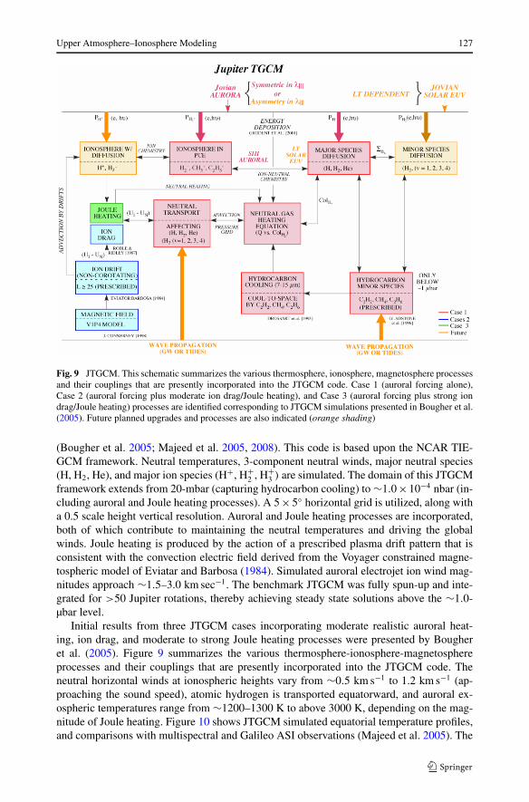
Fig. 9 JTGCM. This schematic summarizes the various thermosphere, ionosphere, magnetosphere processesand their couplings that are presently incorporated into the JTGCM code. Case 1 (auroral forcing alone),Case 2 (auroral forcing plus moderate ion drag/Joule heating), and Case 3 (auroral forcing plus strong iondrag/Joule heating) processes are identified corresponding to JTGCM simulations presented in Bougher et al.(2005). Future planned upgrades and processes are also indicated (orange shading)
(Bougher et al. 2005; Majeed et al. 2005, 2008). This code is based upon the NCAR TIE-GCM framework. Neutral temperatures, 3-component neutral winds, major neutral species(H, H2, He), and major ion species (H+, H+
2 , H+3 ) are simulated. The domain of this JTGCM
framework extends from 20-mbar (capturing hydrocarbon cooling) to ∼1.0×10⁻⁴ nbar (in-cluding auroral and Joule heating processes). A 5 × 5◦ horizontal grid is utilized, along witha 0.5 scale height vertical resolution. Auroral and Joule heating processes are incorporated,both of which contribute to maintaining the neutral temperatures and driving the globalwinds. Joule heating is produced by the action of a prescribed plasma drift pattern that isconsistent with the convection electric field derived from the Voyager constrained magne-tospheric model of Eviatar and Barbosa (1984). Simulated auroral electrojet ion wind mag-nitudes approach ∼1.5–3.0 km sec−1. The benchmark JTGCM was fully spun-up and inte-grated for >50 Jupiter rotations, thereby achieving steady state solutions above the ∼1.0-µbar level.
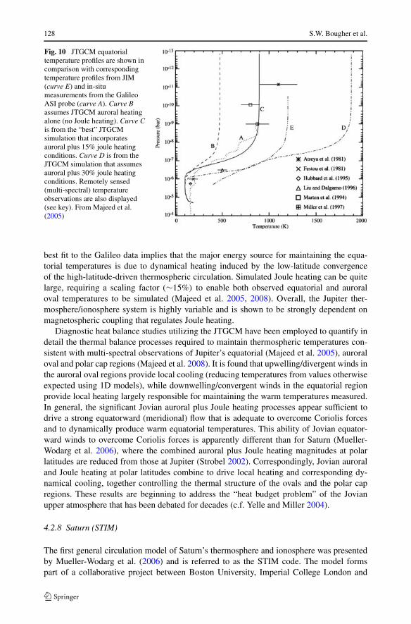
Initial results from three JTGCM cases incorporating moderate realistic auroral heat-ing, ion drag, and moderate to strong Joule heating processes were presented by Bougheret al. (2005). Figure 9 summarizes the various thermosphere-ionosphere-magnetosphereprocesses and their couplings that are presently incorporated into the JTGCM code. Theneutral horizontal winds at ionospheric heights vary from ∼0.5 km s−1 to 1.2 km s−1 (ap-proaching the sound speed), atomic hydrogen is transported equatorward, and auroral ex-ospheric temperatures range from ∼1200–1300 K to above 3000 K, depending on the mag-nitude of Joule heating. Figure 10 shows JTGCM simulated equatorial temperature profiles,and comparisons with multispectral and Galileo ASI observations (Majeed et al. 2005). The
128 S.W. Bougher et al.
Fig. 10 JTGCM equatorialtemperature profiles are shown incomparison with correspondingtemperature profiles from JIM(curve E) and in-situmeasurements from the GalileoASI probe (curve A). Curve Bassumes JTGCM auroral heatingalone (no Joule heating). Curve Cis from the “best” JTGCMsimulation that incorporatesauroral plus 15% joule heatingconditions. Curve D is from theJTGCM simulation that assumesauroral plus 30% joule heatingconditions. Remotely sensed(multi-spectral) temperatureobservations are also displayed(see key). From Majeed et al.(2005)
best fit to the Galileo data implies that the major energy source for maintaining the equa-torial temperatures is due to dynamical heating induced by the low-latitude convergenceof the high-latitude-driven thermospheric circulation. Simulated Joule heating can be quitelarge, requiring a scaling factor (∼15%) to enable both observed equatorial and auroraloval temperatures to be simulated (Majeed et al. 2005, 2008). Overall, the Jupiter ther-mosphere/ionosphere system is highly variable and is shown to be strongly dependent onmagnetospheric coupling that regulates Joule heating.
Diagnostic heat balance studies utilizing the JTGCM have been employed to quantify indetail the thermal balance processes required to maintain thermospheric temperatures con-sistent with multi-spectral observations of Jupiter’s equatorial (Majeed et al. 2005), auroraloval and polar cap regions (Majeed et al. 2008). It is found that upwelling/divergent winds inthe auroral oval regions provide local cooling (reducing temperatures from values otherwiseexpected using 1D models), while downwelling/convergent winds in the equatorial regionprovide local heating largely responsible for maintaining the warm temperatures measured.In general, the significant Jovian auroral plus Joule heating processes appear sufficient todrive a strong equatorward (meridional) flow that is adequate to overcome Coriolis forcesand to dynamically produce warm equatorial temperatures. This ability of Jovian equator-ward winds to overcome Coriolis forces is apparently different than for Saturn (Mueller-Wodarg et al. 2006), where the combined auroral plus Joule heating magnitudes at polarlatitudes are reduced from those at Jupiter (Strobel 2002). Correspondingly, Jovian auroraland Joule heating at polar latitudes combine to drive local heating and corresponding dy-namical cooling, together controlling the thermal structure of the ovals and the polar capregions. These results are beginning to address the “heat budget problem” of the Jovianupper atmosphere that has been debated for decades (c.f. Yelle and Miller 2004).
4.2.8 Saturn (STIM)
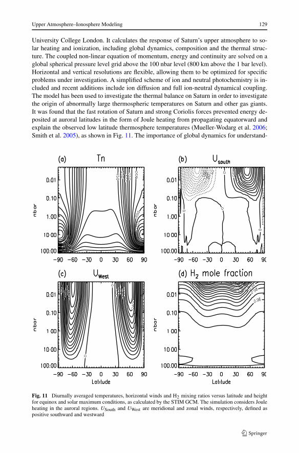
The first general circulation model of Saturn’s thermosphere and ionosphere was presentedby Mueller-Wodarg et al. (2006) and is referred to as the STIM code. The model formspart of a collaborative project between Boston University, Imperial College London and
Upper Atmosphere–Ionosphere Modeling 129
University College London. It calculates the response of Saturn’s upper atmosphere to so-lar heating and ionization, including global dynamics, composition and the thermal struc-ture. The coupled non-linear equation of momentum, energy and continuity are solved on aglobal spherical pressure level grid above the 100 nbar level (800 km above the 1 bar level).Horizontal and vertical resolutions are flexible, allowing them to be optimized for specificproblems under investigation. A simplified scheme of ion and neutral photochemistry is in-cluded and recent additions include ion diffusion and full ion-neutral dynamical coupling.The model has been used to investigate the thermal balance on Saturn in order to investigatethe origin of abnormally large thermospheric temperatures on Saturn and other gas giants.It was found that the fast rotation of Saturn and strong Coriolis forces prevented energy de-posited at auroral latitudes in the form of Joule heating from propagating equatorward andexplain the observed low latitude thermosphere temperatures (Mueller-Wodarg et al. 2006;Smith et al. 2005), as shown in Fig. 11. The importance of global dynamics for understand-
Fig. 11 Diurnally averaged temperatures, horizontal winds and H2 mixing ratios versus latitude and heightfor equinox and solar maximum conditions, as calculated by the STIM GCM. The simulation considers Jouleheating in the auroral regions. USouth and UWest are meridional and zonal winds, respectively, defined aspositive southward and westward
130 S.W. Bougher et al.
ing the thermal balance on gas giants such as Saturn makes the use of general circulationmodels particularly relevant there. Other studies with the ionospheric module of STIM in-vestigated the global structure of Saturn’s highly variable ionosphere, considering shadow-ing by Saturn’s rings (Moore et al. 2004) and effects of water precipitating into Saturn’sionosphere from the rings (Moore et al. 2006). These calculations found the presence of wa-ter to be important to reproduce the dawn dusk asymmetries in electron densities observedby the Cassini Radio Science experiment (Nagy et al. 2006). A recent study by Moore andMendillo (2007) proposed variable water influx rates to be responsible for the high variabil-ity of Saturn’s ionospheric densities.
4.2.9 Titan (TTGCM)
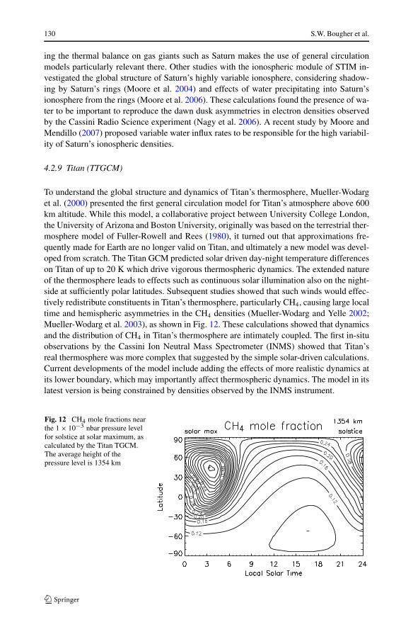
To understand the global structure and dynamics of Titan’s thermosphere, Mueller-Wodarget al. (2000) presented the first general circulation model for Titan’s atmosphere above 600km altitude. While this model, a collaborative project between University College London,the University of Arizona and Boston University, originally was based on the terrestrial ther-mosphere model of Fuller-Rowell and Rees (1980), it turned out that approximations fre-quently made for Earth are no longer valid on Titan, and ultimately a new model was devel-oped from scratch. The Titan GCM predicted solar driven day-night temperature differenceson Titan of up to 20 K which drive vigorous thermospheric dynamics. The extended natureof the thermosphere leads to effects such as continuous solar illumination also on the night-side at sufficiently polar latitudes. Subsequent studies showed that such winds would effec-tively redistribute constituents in Titan’s thermosphere, particularly CH4, causing large localtime and hemispheric asymmetries in the CH4 densities (Mueller-Wodarg and Yelle 2002;Mueller-Wodarg et al. 2003), as shown in Fig. 12. These calculations showed that dynamicsand the distribution of CH4 in Titan’s thermosphere are intimately coupled. The first in-situobservations by the Cassini Ion Neutral Mass Spectrometer (INMS) showed that Titan’sreal thermosphere was more complex that suggested by the simple solar-driven calculations.Current developments of the model include adding the effects of more realistic dynamics atits lower boundary, which may importantly affect thermospheric dynamics. The model in itslatest version is being constrained by densities observed by the INMS instrument.
Fig. 12 CH4 mole fractions nearthe 1 × 10⁻³ nbar pressure levelfor solstice at solar maximum, ascalculated by the Titan TGCM.The average height of thepressure level is 1354 km
Upper Atmosphere–Ionosphere Modeling 131
5 Modeling Frontiers and Problems
5.1 Lower to Upper Atmosphere Coupling
Properly addressing the coupling of the lower and upper atmospheres of planetary environ-ments is a difficult modeling task. “Whole atmosphere” models are ultimately required tocapture the physical processes (e.g., thermal, chemical, dynamical) throughout the entire at-mosphere from the ground to the exobase. However, diffusion processes are much differentabove and below the homopause, requiring a method to be employed to bridge the transitionbetween the homosphere and heterosphere regions. In addition, timescales for chemical andradiative processes vary greatly throughout the atmosphere, typically requiring small time-steps within finite-difference codes. Numerical stability (while utilizing longer time-steps)can be achieved in a number of ways; e.g., by employing implicit solvers and various nu-merical filters. Finally, exercising of multi-dimensional codes on multi-processor computerscan also reduce the wall clock time for global simulations.
5.1.1 Separate but Coupled Model Frameworks vs. Whole Atmosphere Model Frameworks
Two approaches have been employed to date to capture the physics of the entire atmosphere(ground to exobase): (a) coupling of separate lower and upper atmosphere codes; and (b) sin-gle framework “whole atmosphere” model codes. Each approach has advantages and dis-advantages. The coupling of separate codes permits the unique physical processes (andtimescales) of the lower and upper atmospheres to be addressed separately within codeswhich can be optimized for this purpose. Molecular diffusion is one example for the upperatmosphere, for which an implicit (vertical) formulation permits a longer model time-step tobe used. However, linking two separate models across an interface is not “seamless”. By thiswe refer to the lack of an exact match of thermal and dynamical processes (e.g., solar heat-ing, IR cooling, diffusion, numerical filtering) across this interface. Furthermore, both up-ward and downward coupling (i.e., constituent fluxes) is not easily activated across separatemodels. Whole atmosphere models obviate the need for an “artificial” boundary between2-separate codes, while at the same time providing a continuous application of processesthroughout the ground to exobase model domain. Small time-steps may be needed to ac-commodate disparate processes and their timescales throughout the model domain. Finally,whole atmosphere model simulations can be visualized from “top to bottom” with a singlepost-processor.
Examples of both modeling approaches are presented: (Sect. 5.1.2) the whole atmospheremodel approach for Earth (NCAR WACCM), (Sect. 5.1.3) the coupled separate model ap-proach for Mars (NASA MGCM and NCAR MTGCM), and (Sect. 5.1.4) the upward ex-tended LMD-MGCM. The coupled model approach for Mars is a precursor to new Marswhole atmosphere models that are presently being developed and validated (see Table 1; seeSects. 4.2.3 and 5.1.4).
5.1.2 NCAR WACCM (Earth)
The WACCM model version 3 (WACCM3) is a state-of-the-art climate model developed atNCAR that extends from the Earth’s surface to the lower thermosphere. This model is an out-growth of three independent models developed separately across three divisions at NCAR.It combines the major features of these three independently developed models of the at-mosphere, the Middle Atmosphere Community Climate Model (MACCM) (Boville 1995),
132 S.W. Bougher et al.
the chemical model MOZART (Brasseur et al. 1998) and the TIME-GCM (Roble 2000).This model is one of the few high-top general circulation models that include the HamburgModel of the Neutral and Ionized Atmosphere (HAMMONIA) (Schmidt et al. 2006) andthe extended Canadian Middle Atmosphere Model (CMAM) (Fomichev et al. 2002). Thesemodels have been used to study problems such as the solar influence on Earth’s climate, con-stituent transport and trends in the middle atmosphere, the influence of the stratosphere onthe tropospheric climate and the connection between climate change and polar mesosphericclouds. WACCM3 extends between the surface and the lower thermosphere near 140 km.But work is now progressing to move the upper boundary to 500–700 km by incorporatingthe aeronomy of the thermosphere and ionosphere from the TIME-GCM into an upwardextended WACCM.
A number of studies are underway with this new model but one, Sassi et al. (2004),showed a coupling between El-Nino/Lanina ocean influences on the stratosphere/meso-sphere region and another (Richter et al. 2008) showed the importance of gravity waveforcing on the basic structure of the upper atmosphere. Details of the model can be found onthe web site http://www.cgd.ucar.edu/research/models/waccm.html.
5.1.3 NCAR Coupled MGCM-MTGCM (Mars)
The coupled NASA Ames MGCM and the NCAR MTGCM models constitute a numericalframework of 2-independent multi-dimensional codes linked across an interface at 1.32-microbars (∼60–80 km) in the Mars atmosphere (see Sect. 4.2.5). This coupled configura-tion permits both thermal and large scale dynamical processes to be linked across the lowerand upper atmospheres of Mars (e.g., Bougher et al. 2004, 2006b). The 2-model treatmentis designed to be a testbed for addressing coupling processes in advance of the develop-ment and validation of a comprehensive Mars “whole atmosphere” model framework (e.g.Sect. 4.2.3).
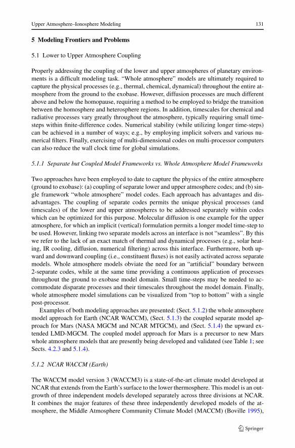
The coupled MGCM-MTGCM system itself has been used successfully to address/interpret an assortment of spacecraft observations, including Mars Global Surveyor, 2001Mars Odyssey, and Mars Reconnaissance Orbiter thermosphere and/or ionosphere data sets(Bougher et al. 1999b, 2000, 2004, 2006b). For example, the recently discovered winterpolar warming features of the Mars lower thermosphere (∼100–130 km) are found to varygreatly over the Mars seasons (e.g., Keating et al. 2003; Bougher et al. 2006b). Figure 13 il-lustrates coupled MGCM-MTGCM simulations for Ls = 90 (aphelion) and 270 (perihelion)conditions, demonstrating that the basic features of the Martian thermospheric winter polarwarming are controlled by seasonal changes in the solar plus tidal forcing, the correspond-ing variations in the strength of the inter-hemispheric Hadley circulation, and the resultingchanges in the magnitude of the adiabatic heating near the winter poles. Calculations of polarwarming show that perihelion adiabatic heating can be highly variable from one Mars year tothe next, and more than twice as strong as that for aphelion conditions (Bougher et al. 2006b;Bell et al. 2007). Finally, without the deep inter-hemispheric Hadley circulation made pos-sible using these coupled lower and upper atmosphere simulations, winter polar warmingfeatures in the Mars thermosphere would not be reproduced at all (Bell et al. 2007).
Several studies are underway utilizing this coupled MGCM-MTGCM framework. Forexample, the role of interannual variations in horizontal and vertical dust distributions in af-fecting the thermospheric temperature and wind distributions is being investigated. Factorsinfluencing the seasonal variation in the Mars mesopause heights and minimum tempera-tures are also being determined (McDunn et al. 2007, 2008).
Upper Atmosphere–Ionosphere Modeling 133
Fig. 13 MGCM-MTGCM zonal averaged temperature slices as a function of height and latitude: (a) Ls = 90and (b) Ls = 270. Contour intervals are 10 K. Color shading is coordinated between these plots. FromBougher et al. (2006b)
5.1.4 LMD-MGCM (Mars)
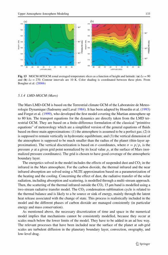
The Mars LMD-GCM is based on the Terrestrial climate GCM of the Laboratoire de Meteo-rologie Dynamique (Sadourny and Laval 1984). It has been adapted by Hourdin et al. (1993)and Forget et al. (1999), who developed the first model covering the Martian atmosphere upto 80 km. The transport equations for the dynamics are directly taken from the LMD ter-restrial GCM. They are based on a finite-difference formulation of the classical “primitiveequations” of meteorology which are a simplified version of the general equations of fluidsbased on three main approximations: (1) the atmosphere is assumed to be a perfect gas; (2) itis supposed to remain vertically in hydrostatic equilibrium; and (3) the vertical dimension ofthe atmosphere is supposed to be much smaller than the radius of the planet (thin-layer ap-proximation). The vertical discretization is based on σ -coordinates, where σ = p/ps is thepressure p at a given grid point normalized by its local value ps at the surface of Mars (nor-malized pressure coordinates). The grid is chosen to have good coverage of the atmosphericboundary layer.
The energetics solved in the model includes the effects of suspended dust and CO2 in theinfrared in the Mars atmosphere. For the carbon dioxide, the thermal infrared and the nearinfrared absorption are solved using a NLTE approximation based on a parameterization ofthe heating and the cooling. Concerning the effect of dust, the radiative transfer of the solarradiation, including absorption and scattering, is modelled through a multi-stream approach.Then, the scattering of the thermal infrared outside the CO2 15 µm band is modelled using atwo-stream radiative transfer model. The CO2 condensation-sublimation cycle is related tothe thermal balance and is likely to a be source or sink of energy, mainly through the latentheat release associated with the change of state. This process is realistically included in themodel and the different phases of carbon dioxide are managed consistently (in particularenergy and mass conservation).
As mentioned above, the necessary discretization of time and space in the numericalmodel implies that mechanisms cannot be consistently modelled, because they occur atscales much below the lower limits of the model. They have to be added in an ad hoc way.The relevant processes that have been included near the surface of the planet at sub-gridscales are turbulent diffusion in the planetary boundary layer, convection, orography, andlow-level drag.
134 S.W. Bougher et al.
Fig. 14 Difference of temperatures between an LMD-GCM simulation without photochemistry and a simu-lation with photochemistry
The LMD-GCM extension to the thermosphere and the exosphere is a collaborative workwith the University of Oxford and the Instituto de Astrofísicade Andalucía. The model hasbeen successively extended from the ground up to a height of approximately 120 km (Ange-lats i Coll et al. 2003), 240 km (González-Galindo et al. 2004) and finally up to the exosphere(González-Galindo et al. 2007). The extension to the upper altitudes has been done in sucha way that the processes that are important either in the mesosphere or in the thermosphereare taken into account.
In rarefied regions (thermospheres), each component of the neutral gas has an individ-ual behaviour, which can be modelled using the Enskog approach, because this region isstill collision dominated. We must distinguish horizontal from vertical dynamics, since thetemporal and spatial scales are different. Temperature can be assumed to be the same forall the species, so a single equation for the temperature, which accounts for the thermalconductivity of the mean gas and the UV heating can be used. We do the same for the hor-izontal velocity, using a mean molecular viscosity. However, vertical diffusion is importantin the upper atmosphere, and a multi-species Chapman-Enskog approach is used for multi-component diffusion.
At upper altitudes, it is demonstrated that photochemistry becomes a very important fea-ture of the atmospheric dynamics. A 1-D photochemical model using a complex photo-chemistry scheme, which includes the 12 major constituents of the C, O and H families, andaccounts for 27 reactions between them has been developed and included in the LMD-GCMmodel. Figure 14 shows the impact that the photochemistry may have on the energy balancein the thermosphere. Temperature differences up to 35 K can be obtained above 200 km ifsome chemical processes are neglected.
The infrared processes related to CO2, already mentioned above, are relevant processesfor the mesosphere, and strongly NLTE in that region. Some approximation and parameteri-zation has been done to include them, without increasing dramatically the computation time.The main heating source of the Martian thermosphere is the UV heating. In order to be able
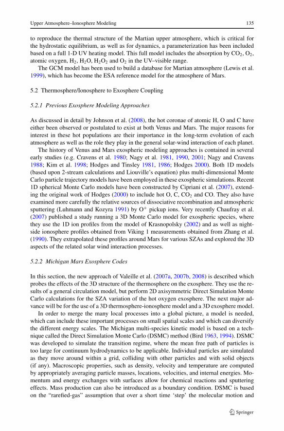
Upper Atmosphere–Ionosphere Modeling 135
to reproduce the thermal structure of the Martian upper atmosphere, which is critical forthe hydrostatic equilibrium, as well as for dynamics, a parameterization has been includedbased on a full 1-D UV heating model. This full model includes the absorption by CO2, O2,atomic oxygen, H2, H2O, H2O2 and O2 in the UV–visible range.
The GCM model has been used to build a database for Martian atmosphere (Lewis et al.1999), which has become the ESA reference model for the atmosphere of Mars.
5.2 Thermosphere/Ionosphere to Exosphere Coupling
5.2.1 Previous Exosphere Modeling Approaches
As discussed in detail by Johnson et al. (2008), the hot coronae of atomic H, O and C haveeither been observed or postulated to exist at both Venus and Mars. The major reasons forinterest in these hot populations are their importance in the long-term evolution of eachatmosphere as well as the role they play in the general solar-wind interaction of each planet.
The history of Venus and Mars exospheric modeling approaches is contained in severalearly studies (e.g. Cravens et al. 1980; Nagy et al. 1981, 1990, 2001; Nagy and Cravens1988; Kim et al. 1998; Hodges and Tinsley 1981, 1986; Hodges 2000). Both 1D models(based upon 2-stream calculations and Liouville’s equation) plus multi-dimensional MonteCarlo particle trajectory models have been employed in these exospheric simulations. Recent1D spherical Monte Carlo models have been constructed by Cipriani et al. (2007), extend-ing the original work of Hodges (2000) to include hot O, C, CO2 and CO. They also haveexamined more carefully the relative sources of dissociative recombination and atmosphericsputtering (Luhmann and Kozyra 1991) by O+ pickup ions. Very recently Chaufray et al.(2007) published a study running a 3D Monte Carlo model for exospheric species, wherethey use the 1D ion profiles from the model of Krasnopolsky (2002) and as well as night-side ionosphere profiles obtained from Viking 1 measurements obtained from Zhang et al.(1990). They extrapolated these profiles around Mars for various SZAs and explored the 3Daspects of the related solar wind interaction processes.
5.2.2 Michigan Mars Exosphere Codes
In this section, the new approach of Valeille et al. (2007a, 2007b, 2008) is described whichprobes the effects of the 3D structure of the thermosphere on the exosphere. They use the re-sults of a general circulation model, but perform 2D axisymmetric Direct Simulation MonteCarlo calculations for the SZA variation of the hot oxygen exosphere. The next major ad-vance will be for the use of a 3D thermosphere-ionosphere model and a 3D exosphere model.
In order to merge the many local processes into a global picture, a model is needed,which can include these important processes on small spatial scales and which can diversifythe different energy scales. The Michigan multi-species kinetic model is based on a tech-nique called the Direct Simulation Monte Carlo (DSMC) method (Bird 1963, 1994). DSMCwas developed to simulate the transition regime, where the mean free path of particles istoo large for continuum hydrodynamics to be applicable. Individual particles are simulatedas they move around within a grid, colliding with other particles and with solid objects(if any). Macroscopic properties, such as density, velocity and temperature are computedby appropriately averaging particle masses, locations, velocities, and internal energies. Mo-mentum and energy exchanges with surfaces allow for chemical reactions and sputteringeffects. Mass production can also be introduced as a boundary condition. DSMC is basedon the “rarefied-gas” assumption that over a short time ‘step’ the molecular motion and
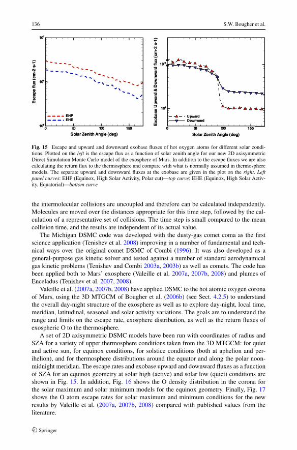
136 S.W. Bougher et al.
Fig. 15 Escape and upward and downward exobase fluxes of hot oxygen atoms for different solar condi-tions. Plotted on the left is the escape flux as a function of solar zenith angle for our new 2D axisymmetricDirect Simulation Monte Carlo model of the exosphere of Mars. In addition to the escape fluxes we are alsocalculating the return flux to the thermosphere and compare with what is normally assumed in thermospheremodels. The separate upward and downward fluxes at the exobase are given in the plot on the right. Leftpanel curves: EHP (Equinox, High Solar Activity, Polar cut)—top curve; EHE (Equinox, High Solar Activ-ity, Equatorial)—bottom curve
the intermolecular collisions are uncoupled and therefore can be calculated independently.Molecules are moved over the distances appropriate for this time step, followed by the cal-culation of a representative set of collisions. The time step is small compared to the meancollision time, and the results are independent of its actual value.
The Michigan DSMC code was developed with the dusty-gas comet coma as the firstscience application (Tenishev et al. 2008) improving in a number of fundamental and tech-nical ways over the original comet DSMC of Combi (1996). It was also developed as ageneral-purpose gas kinetic solver and tested against a number of standard aerodynamicalgas kinetic problems (Tenishev and Combi 2003a, 2003b) as well as comets. The code hasbeen applied both to Mars’ exosphere (Valeille et al. 2007a, 2007b, 2008) and plumes ofEnceladus (Tenishev et al. 2007, 2008).
Valeille et al. (2007a, 2007b, 2008) have applied DSMC to the hot atomic oxygen coronaof Mars, using the 3D MTGCM of Bougher et al. (2006b) (see Sect. 4.2.5) to understandthe overall day-night structure of the exosphere as well as to explore day-night, local time,meridian, latitudinal, seasonal and solar activity variations. The goals are to understand therange and limits on the escape rate, exosphere distribution, as well as the return fluxes ofexospheric O to the thermosphere.
A set of 2D axisymmetric DSMC models have been run with coordinates of radius andSZA for a variety of upper thermosphere conditions taken from the 3D MTGCM: for quietand active sun, for equinox conditions, for solstice conditions (both at aphelion and per-ihelion), and for thermosphere distributions around the equator and along the polar noon-midnight meridian. The escape rates and exobase upward and downward fluxes as a functionof SZA for an equinox geometry at solar high (active) and solar low (quiet) conditions areshown in Fig. 15. In addition, Fig. 16 shows the O density distribution in the corona forthe solar maximum and solar minimum models for the equinox geometry. Finally, Fig. 17shows the O atom escape rates for solar maximum and minimum conditions for the newresults by Valeille et al. (2007a, 2007b, 2008) compared with published values from theliterature.
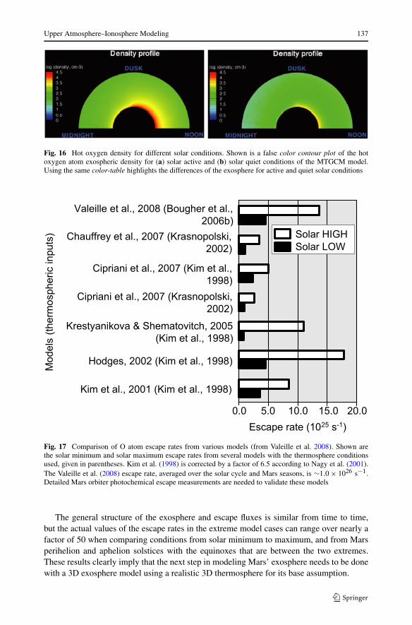
Upper Atmosphere–Ionosphere Modeling 137
Fig. 16 Hot oxygen density for different solar conditions. Shown is a false color contour plot of the hotoxygen atom exospheric density for (a) solar active and (b) solar quiet conditions of the MTGCM model.Using the same color-table highlights the differences of the exosphere for active and quiet solar conditions
Fig. 17 Comparison of O atom escape rates from various models (from Valeille et al. 2008). Shown arethe solar minimum and solar maximum escape rates from several models with the thermosphere conditionsused, given in parentheses. Kim et al. (1998) is corrected by a factor of 6.5 according to Nagy et al. (2001).The Valeille et al. (2008) escape rate, averaged over the solar cycle and Mars seasons, is ∼1.0 × 1026 s−1.Detailed Mars orbiter photochemical escape measurements are needed to validate these models
The general structure of the exosphere and escape fluxes is similar from time to time,but the actual values of the escape rates in the extreme model cases can range over nearly afactor of 50 when comparing conditions from solar minimum to maximum, and from Marsperihelion and aphelion solstices with the equinoxes that are between the two extremes.These results clearly imply that the next step in modeling Mars’ exosphere needs to be donewith a 3D exosphere model using a realistic 3D thermosphere for its base assumption.
138 S.W. Bougher et al.
References
N. Achilleos, S. Miller, J. Tennyson, A. Aylward, I. Mueller-Wodarg, D. Rees, J. Geophys. Res. 103, 20089–20112 (1998). doi:10.1029/98JE00947
N. Achilleos, S. Miller, R. Prangé, G. Millward, M.K. Dougherty, N.J. Phys. 3 (2001). doi:10.1088/1367-2630/3/1/303
M. Angelats i Coll, F. Forget, M.A. López-Valverde, P.L. Read, S.R. Lewis, J. Geophys. Res. 109, 1011(2003). doi:10.1029/2003JE002163
J.M. Bell, The dynamics of the upper atmospheres of Mars and Titan. Ph.D Thesis, University of Michigan(2008)
J.M. Bell, S.W. Bougher, V. De LaHaye, J.H. Waite Jr., A. Ridley, Eos Trans. Am. Geophys. Union 87(Jt.Assem. Suppl.) (2006), abstract U52A-06
J.M. Bell, S.W. Bougher, J.R. Murphy, J. Geophys. Res. 112, E12002 (2007). doi:10/1029/2006JE002856J.-L. Bertaux et al., Science 307, 566–569 (2005)G.A. Bird, Phys. Fluids 6, 1518–1519 (1963)G.A. Bird, Molecular Gas Dynamics and the Direct Simulations of Gas Flows (Clarendon, Oxford, 1994)V. Boqueho, P.-L. Blelly, J. Geophys. Res. 110, A01313 (2005). doi:10.1029/2004JA010414S.W. Bougher et al., Icarus 68, 284–312 (1986)S.W. Bougher, R.E. Dickinson, E.C. Ridley, R.G. Roble, Icarus 73, 545–573 (1988)S.W. Bougher, J.C. Gerard, A.I.F. Stewart, C.G. Fesen, J. Geophys. Res. 95, 6271–6284 (1990)S.W. Bougher, W.J. Borucki, J. Geophys. Res. 99, 3759–3776 (1994)S.W. Bougher, D.M. Hunten, R.G. Roble, J. Geophys. Res. 99, 14609–14622 (1994)S.W. Bougher, M.J. Alexander, H.G. Mayr, in Venus II, ed. by S.W. Bougher, D.M. Hunten, R.J. Philips
(University of Arizona Press, Tucson, 1997), pp. 259–292S.W. Bougher, S. Engel, R.G. Roble, B. Foster, J. Geophys. Res. 104, 16591–16611 (1999a)S.W. Bougher et al., Adv. Space Res. 23(11), 1887–1897 (1999b)S.W. Bougher, S. Engel, R.G. Roble, B. Foster, J. Geophys. Res. 105, 17,669–17,689 (2000)S.W. Bougher, R.G. Roble, T.J. Fuller-Rowell, in Atmospheres in the Solar System: Comparative Aeronomy,
ed. by M. Mendillo, A. Nagy, H. Waite. Geophysical Monograph, vol. 130 (American GeophysicalUnion, Washington, 2002), pp. 261–288
S.W. Bougher, S. Engel, D.P. Hinson, J.R. Murphy, J. Geophys. Res. 109, E03010 (2004). doi:10.1029/2003JE002154
S.W. Bougher, J.H. Waite, T. Majeed, G.R. Gladstone, J. Geophys. Res. 110, E04008 (2005). doi:10.1029/2003JE002230
S.W. Bougher, S. Rafkin, P. Drossart, Planet. Space Sci. 54, 1371–1380 (2006a)S.W. Bougher, J.M. Bell, J.R. Murphy, M.A. López-Valverde, P.G. Withers, Geophys. Res. Lett. 33, L02203
(2006b). doi:10.1029/2005GL024059S.W. Bougher, A. Brecht, C. Parkinson, S. Rafkin, B. Foster, 37th COSPAR Scientific Assembly 2008, C32-
0003-08 Abstract (2008)B.A. Boville, J. Geophys. Res. 100, 9017–9039 (1995)G.P. Brasseur et al., J. Geophys. Res. 103, 28265–28290 (1998)A. Brecht, S.W. Bougher, S. Rafkin, B. Foster, Eos Trans. Am. Geophys. Union 88(52), (Fall Meeting Suppl.)
(2007), abstract P33B-1299J.Y. Chaufray et al., J. Geophys. Res. 112, E09009 (2007). doi:10.1029/2007JE002915R.H. Chen, A.F. Nagy, J. Geophys. Res. 83, 1133–1140 (1978)R.H. Chen, T.E. Cravens, A.F. Nagy, J. Geophys. Res. 83, 3871–3876 (1978)F. Cipriani, F. Leblanc, J.J. Berthelier, J. Geophys. Res. 112, D07001 (2007). doi:10.1029/2006JE002818M.R. Combi, Icarus 123, 207–226 (1996)T.E. Cravens, T.I. Gombosi, A.F. Nagy, Nature 283, 178–180 (1980)T.E. Cravens, A.J. Kliore, J.U. Kozyra, A.F. Nagy, J. Geophys. Res. 86, 11,323–11,329 (1981)V. DeLa Haye, Coronal formation and heating efficiencies in Titan’s upper atmosphere: Construction of a
coupled ion, neutral and thermal structure model to interpret the first INMS Cassini data. Ph.D. Thesis,University of Michigan, Ann Arbor (2005)
Y. Deng, A.D. Richmond, A.J. Ridley, H. Liu, Geophys. Res. Lett. 35, L01104 (2008). doi:10.1029/2007GL032182
A.L. Dobbin, A.D. Aylward, M.J. Harris, J. Geophys. Res. 111, A07314 (2006). doi:10.1029/2005JA011543A. Eviatar, A.D. Barbosa, J. Geophys. Res. 89, 7393–7398 (1984)P.R. Field et al., J. Atmos. Sol. Terr. Phys. 60, 523–543 (1998)M.O. Fillingim et al., Geophys. Res. Lett. 34, L12101 (2007). doi:10.1029/2007GL029986V.I. Fomichev et al., J. Geophys. Res. 107 (2002). doi:1029/2001JD000479
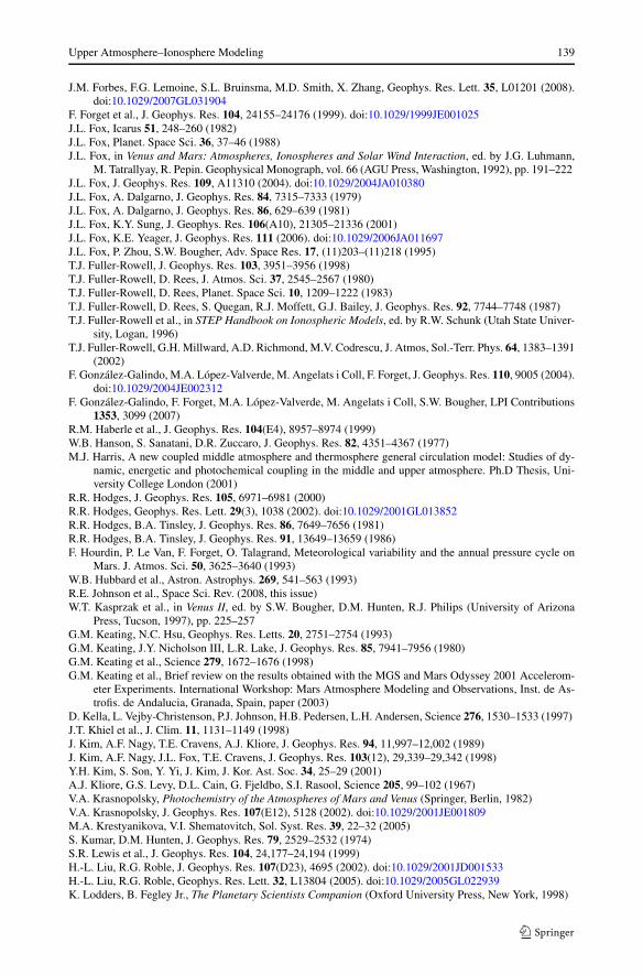
Upper Atmosphere–Ionosphere Modeling 139
J.M. Forbes, F.G. Lemoine, S.L. Bruinsma, M.D. Smith, X. Zhang, Geophys. Res. Lett. 35, L01201 (2008).doi:10.1029/2007GL031904
F. Forget et al., J. Geophys. Res. 104, 24155–24176 (1999). doi:10.1029/1999JE001025J.L. Fox, Icarus 51, 248–260 (1982)J.L. Fox, Planet. Space Sci. 36, 37–46 (1988)J.L. Fox, in Venus and Mars: Atmospheres, Ionospheres and Solar Wind Interaction, ed. by J.G. Luhmann,
M. Tatrallyay, R. Pepin. Geophysical Monograph, vol. 66 (AGU Press, Washington, 1992), pp. 191–222J.L. Fox, J. Geophys. Res. 109, A11310 (2004). doi:10.1029/2004JA010380J.L. Fox, A. Dalgarno, J. Geophys. Res. 84, 7315–7333 (1979)J.L. Fox, A. Dalgarno, J. Geophys. Res. 86, 629–639 (1981)J.L. Fox, K.Y. Sung, J. Geophys. Res. 106(A10), 21305–21336 (2001)J.L. Fox, K.E. Yeager, J. Geophys. Res. 111 (2006). doi:10.1029/2006JA011697J.L. Fox, P. Zhou, S.W. Bougher, Adv. Space Res. 17, (11)203–(11)218 (1995)T.J. Fuller-Rowell, J. Geophys. Res. 103, 3951–3956 (1998)T.J. Fuller-Rowell, D. Rees, J. Atmos. Sci. 37, 2545–2567 (1980)T.J. Fuller-Rowell, D. Rees, Planet. Space Sci. 10, 1209–1222 (1983)T.J. Fuller-Rowell, D. Rees, S. Quegan, R.J. Moffett, G.J. Bailey, J. Geophys. Res. 92, 7744–7748 (1987)T.J. Fuller-Rowell et al., in STEP Handbook on Ionospheric Models, ed. by R.W. Schunk (Utah State Univer-
sity, Logan, 1996)T.J. Fuller-Rowell, G.H. Millward, A.D. Richmond, M.V. Codrescu, J. Atmos, Sol.-Terr. Phys. 64, 1383–1391
(2002)F. González-Galindo, M.A. López-Valverde, M. Angelats i Coll, F. Forget, J. Geophys. Res. 110, 9005 (2004).
doi:10.1029/2004JE002312F. González-Galindo, F. Forget, M.A. López-Valverde, M. Angelats i Coll, S.W. Bougher, LPI Contributions
1353, 3099 (2007)R.M. Haberle et al., J. Geophys. Res. 104(E4), 8957–8974 (1999)W.B. Hanson, S. Sanatani, D.R. Zuccaro, J. Geophys. Res. 82, 4351–4367 (1977)M.J. Harris, A new coupled middle atmosphere and thermosphere general circulation model: Studies of dy-
namic, energetic and photochemical coupling in the middle and upper atmosphere. Ph.D Thesis, Uni-versity College London (2001)
R.R. Hodges, J. Geophys. Res. 105, 6971–6981 (2000)R.R. Hodges, Geophys. Res. Lett. 29(3), 1038 (2002). doi:10.1029/2001GL013852R.R. Hodges, B.A. Tinsley, J. Geophys. Res. 86, 7649–7656 (1981)R.R. Hodges, B.A. Tinsley, J. Geophys. Res. 91, 13649–13659 (1986)F. Hourdin, P. Le Van, F. Forget, O. Talagrand, Meteorological variability and the annual pressure cycle on
Mars. J. Atmos. Sci. 50, 3625–3640 (1993)W.B. Hubbard et al., Astron. Astrophys. 269, 541–563 (1993)R.E. Johnson et al., Space Sci. Rev. (2008, this issue)W.T. Kasprzak et al., in Venus II, ed. by S.W. Bougher, D.M. Hunten, R.J. Philips (University of Arizona
Press, Tucson, 1997), pp. 225–257G.M. Keating, N.C. Hsu, Geophys. Res. Letts. 20, 2751–2754 (1993)G.M. Keating, J.Y. Nicholson III, L.R. Lake, J. Geophys. Res. 85, 7941–7956 (1980)G.M. Keating et al., Science 279, 1672–1676 (1998)G.M. Keating et al., Brief review on the results obtained with the MGS and Mars Odyssey 2001 Accelerom-
eter Experiments. International Workshop: Mars Atmosphere Modeling and Observations, Inst. de As-trofis. de Andalucia, Granada, Spain, paper (2003)
D. Kella, L. Vejby-Christenson, P.J. Johnson, H.B. Pedersen, L.H. Andersen, Science 276, 1530–1533 (1997)J.T. Khiel et al., J. Clim. 11, 1131–1149 (1998)J. Kim, A.F. Nagy, T.E. Cravens, A.J. Kliore, J. Geophys. Res. 94, 11,997–12,002 (1989)J. Kim, A.F. Nagy, J.L. Fox, T.E. Cravens, J. Geophys. Res. 103(12), 29,339–29,342 (1998)Y.H. Kim, S. Son, Y. Yi, J. Kim, J. Kor. Ast. Soc. 34, 25–29 (2001)A.J. Kliore, G.S. Levy, D.L. Cain, G. Fjeldbo, S.I. Rasool, Science 205, 99–102 (1967)V.A. Krasnopolsky, Photochemistry of the Atmospheres of Mars and Venus (Springer, Berlin, 1982)V.A. Krasnopolsky, J. Geophys. Res. 107(E12), 5128 (2002). doi:10.1029/2001JE001809M.A. Krestyanikova, V.I. Shematovitch, Sol. Syst. Res. 39, 22–32 (2005)S. Kumar, D.M. Hunten, J. Geophys. Res. 79, 2529–2532 (1974)S.R. Lewis et al., J. Geophys. Res. 104, 24,177–24,194 (1999)H.-L. Liu, R.G. Roble, J. Geophys. Res. 107(D23), 4695 (2002). doi:10.1029/2001JD001533H.-L. Liu, R.G. Roble, Geophys. Res. Lett. 32, L13804 (2005). doi:10.1029/2005GL022939K. Lodders, B. Fegley Jr., The Planetary Scientists Companion (Oxford University Press, New York, 1998)
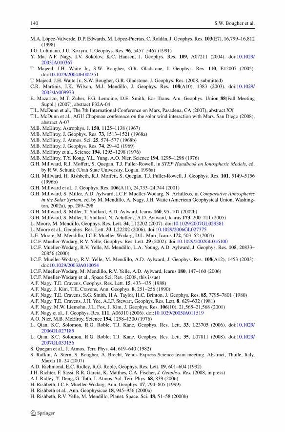
140 S.W. Bougher et al.
M.A. López-Valverde, D.P. Edwards, M. López-Puertas, C. Roldán, J. Geophys. Res. 103(E7), 16,799–16,812(1998)
J.G. Luhmann, J.U. Kozyra, J. Geophys. Res. 96, 5457–5467 (1991)Y. Ma, A.F. Nagy, I.V. Sokolov, K.C. Hansen, J. Geophys. Res. 109, A07211 (2004). doi:10.1029/
2003JA010367T. Majeed, J.H. Waite Jr., S.W. Bougher, G.R. Gladstone, J. Geophys. Res. 110, E12007 (2005).
doi:10.1029/2004JE002351T. Majeed, J.H. Waite Jr., S.W. Bougher, G.R. Gladstone, J. Geophys. Res. (2008, submitted)C.R. Martinis, J.K. Wilson, M.J. Mendillo, J. Geophys. Res. 108(A10), 1383 (2003). doi:10.1029/
2003/JA009973E. Mazarico, M.T. Zuber, F.G. Lemoine, D.E. Smith, Eos Trans. Am. Geophys. Union 88(Fall Meeting
Suppl.) (2007), abstract P32A-04T.L. McDunn et al., The 7th International Conference on Mars, Pasadena, CA (2007), abstract XXT.L. McDunn et al., AGU Chapman conference on the solar wind interaction with Mars. San Diego (2008),
abstract A-07M.B. McElroy, Astrophys. J. 150, 1125–1138 (1967)M.B. McElroy, J. Geophys. Res. 73, 1513–1521 (1968a)M.B. McElroy, J. Atmos. Sci. 25, 574–577 (1968b)M.B. McElroy, J. Geophys. Res. 74, 29–42 (1969)M.B. McElroy et al., Science 194, 1295–1298 (1976)M.B. McElroy, T.Y. Kong, Y.L. Yung, A.O. Nier, Science 194, 1295–1298 (1976)G.H. Millward, R.J. Moffett, S. Quegan, T.J. Fuller-Rowell, in STEP Handbook on Ionospheric Models, ed.
by R.W. Schunk (Utah State University, Logan, 1996a)G.H. Millward, H. Rishbeth, R.J. Moffett, S. Quegan, T.J. Fuller-Rowell, J. Geophys. Res. 101, 5149–5156
(1996b)G.H. Millward et al., J. Geophys. Res. 106(A11), 24,733–24,744 (2001)G.H. Millward, S. Miller, A.D. Aylward, I.C.F. Mueller-Wodarg, N. Achilleos, in Comparative Atmospheres
in the Solar System, ed. by M. Mendillo, A. Nagy, J.H. Waite (American Geophysical Union, Washing-ton, 2002a), pp. 289–298
G.H. Millward, S. Miller, T. Stallard, A.D. Aylward, Icarus 160, 95–107 (2002b)G.H. Millward, S. Miller, T. Stallard, N. Achilleos, A.D. Aylward, Icarus 173, 200–211 (2005)L. Moore, M. Mendillo, Geophys. Res. Lett. 34, L12202 (2007). doi:10.1029/2007GL029381L. Moore et al., Geophys. Res. Lett. 33, L22202 (2006). doi:10.1029/2006GL027375L.E. Moore, M. Mendillo, I.C.F. Mueller-Wodarg, D.L. Murr, Icarus 172, 503–52 (2004)I.C.F. Mueller-Wodarg, R.V. Yelle, Geophys. Res. Lett. 29 (2002). doi:10.1029/2002GL016100I.C.F. Mueller-Wodarg, R.V. Yelle, M. Mendillo, L.A. Young, A.D. Aylward, J. Geophys. Res. 105, 20833–
20856 (2000)I.C.F. Mueller-Wodarg, R.V. Yelle, M. Mendillo, A.D. Aylward, J. Geophys. Res. 108(A12), 1453 (2003).
doi:10.1029/2003JA010054I.C.F. Mueller-Wodarg, M. Mendillo, R.V. Yelle, A.D. Aylward, Icarus 180, 147–160 (2006)I.C.F. Mueller-Wodarg et al., Space Sci. Rev. (2008, this issue)A.F. Nagy, T.E. Cravens, Geophys. Res. Lett. 15, 433–435 (1988)A.F. Nagy, J. Kim, T.E. Cravens, Ann. Geophys. 8, 251–256 (1990)A.F. Nagy, T.E. Cravens, S.G. Smith, H.A. Taylor, H.C. Brinton, J. Geophys. Res. 85, 7795–7801 (1980)A.F. Nagy, T.E. Cravens, J.H. Yee, A.I.F. Stewart, Geophys. Res. Lett. 8, 629–632 (1981)A.F. Nagy, M.W. Liemohn, J.L. Fox, J. Kim, J. Geophys. Res. 106(10), 21,565–21,568 (2001)A.F. Nagy et al., J. Geophys. Res. 111, A06310 (2006). doi:10.1029/2005JA011519A.O. Nier, M.B. McElroy, Science 194, 1298–1300 (1976)L. Qian, S.C. Solomon, R.G. Roble, T.J. Kane, Geophys. Res. Lett. 33, L23705 (2006). doi:10.1029/
2006GL027185L. Qian, S.C. Solomon, R.G. Roble, T.J. Kane, Geophys. Res. Lett. 35, L07811 (2008). doi:10.1029/
2007GL033156S. Quegan et al., J. Atmos. Terr. Phys. 44, 619–640 (1982)S. Rafkin, A. Stern, S. Bougher, A. Brecht, Venus Express Science team meeting. Abstract, Thuile, Italy,
March 18–24 (2007)A.D. Richmond, E.C. Ridley, R.G. Roble, Geophys. Res. Lett. 19, 601–604 (1992)J.H. Richter, F. Sassi, R.R. Garcia, K. Matthes, C.A. Fischer, J. Geophys. Res. (2008, in press)A.J. Ridley, Y. Deng, G. Toth, J. Atmos. Sol. Terr. Phys. 68, 839 (2006)H. Rishbeth, I.C.F. Mueller-Wodarg, Ann. Geophys. 17, 794–805 (1999)H. Rishbeth et al., Ann. Geophysicae 18, 945–956 (2000a)H. Rishbeth, R.V. Yelle, M. Mendillo, Planet. Space. Sci. 48, 51–58 (2000b)
Upper Atmosphere–Ionosphere Modeling 141
R.G. Roble, in The Upper Mesosphere Lower Thermosphere: A Review of Experiment and Theory, ed. byR.M. Johnson, T.L. Killeen. Geophysical Monograph, vol. 87 (American Geophysical Union, 1995),p. 1
R.G. Roble, in Atmospheric Science Across the Stratopause. Geophysical Monograph, vol. 123 (AmericanGeophysical Union, 2000), pp. 53–67
R.G. Roble, R.E. Dickinson, Geophys. Res. Lett. 16, 1441–1444 (1989)R.G. Roble, E.C. Ridley, Geophys. Res. Lett. 21, 417–420 (1994)R.G. Roble, E.C. Ridely, R.E. Dickinson, J. Geophys. Res. 92, 8745–8758 (1987)C. Roldan, M.A. Lopez-Valverde, M. Lopez-Puertas, D.P. Edwards, Icarus 147, 11–25 (2000)R. Sadourny, K. Laval, in New Perspectives in Climate Modeling, ed. by A. Berger, C. Nicolis (Elsevier,
Amsterdam, 1984), pp. 173–197F. Sassi, D. Kinneson, B.A. Boville, R.R. Garcia, R.G. Roble, J. Geophys. Res. 109, D17108 (2004).
doi:10.1029/2003JD004434H.G. Schmidt et al., J. Climate 19 (2006). doi:10.1175/JCLI3829.1G. Schubert et al., in Exploring Venus as a Terrestrial Planet. Geophysical Monograph, vol. 176 (American
Geophysical Union, 2007), pp. 101–120R.W. Schunk, A.F. Nagy, Ionospheres: Physics, Plasma Physics and Chemistry. Cambridge Atmospheric and
Space Science Series (Cambridge University Press, Cambridge, 2000)R. Shimazaki, M. Shimizu, Rep. Ionos. Space Res. Jpn. 24, 80–98 (1970)H. Shinagawa, T.E. Cravens, J. Geophys. Res. 93, 11,263–11,277 (1988)H. Shinagawa, T.E. Cravens, J. Geophys. Res. 94, 6506–6516 (1989)C.G.A. Smith, S. Miller, A.D. Aylward, Ann. Geophys. 23, 1943–1947 (2005)R.W. Stewart, J. Atmos. Sci. 25, 578–582 (1968)R.W. Stewart, J. Atmos. Sci. 28, 1069–1073 (1971)D.F. Strobel, in Atmospheres in the Solar System: Comparative Aeronomy, ed. by M. Mendillo, A. Nagy,
H. Waite. Geophysical Monograph, vol. 130 (American Geophysical Union, Washington, 2002), pp.7–22
V.T. Tenishev, M.R. Combi, AIAA Paper 2003-3776 (2003a)V.T. Tenishev, M.R. Combi, RGD, 23rd Int. Symp. 663, 696 (2003b)V.T. Tenishev, M. Combi, H. Waite, Eos Trans. Am. Geophys. Union 88(23) (Jt. Assem. Suppl.) (2007),
abstract P43A-02V.T. Tenishev, M.R. Combi, B. Davidsson, Astrophys. J. (2008, in press)R.H. Tolson et al., J. Spacecr. Rockets 44(6), 1172–1179 (2007)A. Valeille, V. Tenishev, S.W. Bougher, M.R. Combi, A.F. Nagy, Eos Trans. Am. Geophys. Union 88(23) (Jt.
Assem. Suppl.) (2007a), abstract SA31B-02A. Valeille, V. Tenishev, S.W. Bougher, M.R. Combi, A.F. Nagy, B. A. A. S. 39, #24.01 (2007b)A. Valeille, M.R. Combi, V.T. Tenishev, S.W. Bougher, A.F. Nagy, Icarus (2008, submitted)U. von Zahn et al., J. Geophys. Res. 85, 7829–7840 (1980)J.H. Waite et al., Science 308, 982–986 (2005)O. Witasse et al., Space Sci. Rev. (2008, this issue)P.G. Withers, Geophys. Res. Letts. 33, L02201 (2006). doi:10.1029/2005GL024447R.V. Yelle, S. Miller, in Jupiter: The Planet, Satellites, and Magnetosphere, ed. by F. Bagenal, T.E. Dowling,
W.B. McKinnon (Cambridge Univ. Press, New York, 2004), pp. 185–218M.H.G. Zhang, J.G. Luhmann, A.J. Kliore, J. Kim, J. Geophys. Res. 95, 14829–14839 (1990)S. Zhang, S.W. Bougher, M.J. Alexander, J. Geophys. Res. 101, 23195–23205 (1996)