semiparametric regression models with missing data - university of
TRANSCRIPT
Semiparametric Regression Models withMissing Data: the Mathematics in the Work
of Robins et al.
Menggang Yu and Bin Nan
University of Michigan
May 3, 2003
Abstract
This review is an attempt to understand the landmark papers of Robins,
Rotnitzky, and Zhao (1994) and Robins and Rotnitzky (1992). We revisit
their main results and corresponding proofs using the theory outlined in the monograph
by Bickel, Klaassen, Ritov, and Wellner (1993). We also discuss an illustrative
example to show the details of applying these theoretical results.
Keywords and phrases: Efficient score, influence function, missing at random,
regression models, scores, tangent set, tangent space.
1 Introduction
Improving efficiency for the estimates in semiparametric regression models with missing data
has been an interesting and active research subject. Robins, Rotnitzky, and Zhao (1994)
(hereafter RRZ) provided profound calculations of efficient score functions and information
bounds for models with data Missing At Random (MAR, a terminology of Little and
Rubin (1987)). Part of their calculations can also be found in Robins and Rotnitzky
(1992) (hereafter RR). Their basic idea is to bridge the model with missing data and the
corresponding model without missing data (full model), if certain properties of the full model
1

are known or easily obtained. The results are fundamental and can be applied to a variety of
regression models. But it is very difficult to read these comprehensive abstract results since
the authors only supplied very condensed proofs, and the whole material, including notation,
was organized in a way that is hard to follow. We feel that it is necessary to revisit these very
important results. The purpose of this study is to explicate RRZ and RR using the theory
(and notation) in Bickel, Klaassen, Ritov, and Wellner (1993) (hereafter BKRW). The
desired result is that a wider audience of statisticians interested in semiparametric models
with missing data feel more comfortable following the recent developments in the area and
applying the results in RRZ and RR. We begin by introducing the general semiparametric
model with data MAR and the notation that will be used in the following sections. In Section
3, we introduce the main results of calculations of efficient score functions for data MAR with
arbitrary missing patterns, monotonic missing patterns, and the two-phase sampling designs
which are special cases of monotonic missingness. In Section 4 we discuss a simple example
of the mean regression model with surrogate outcome to show the details of applying the
general results in RRZ and RR. The detailed rigorous proofs of the main results can be found
in Section 5, which is followed by the properties of influence functions and corresponding
proofs in Section 6. We wrap up with a brief discussion in Section 7.
2 A General Model and Notation
We will adopt the notation mostly from Bickel, Klaassen, Ritov, and Wellner (1993)
and Nan, Emond, and Wellner (2000). Suppose the underlying full data are i.i.d. copies
of the m-dimensional random vector X = (X1, . . . , Xm). We denote the model for X as
Q = {Qθ,η : θ ∈ Θ ⊂ Rd, η ∈ H} where Qθ,η is a distribution function, θ is the parameter of
interest and η is an infinite-dimensional nuisance parameter or a vector of several infinite-
dimensional nuisance parameters.
Let R = (R1, . . . , Rm) be a random vector with Rj = 1 if Xj is observed and Rj = 0 if
Xj is missing, j = 1, . . . ,m. Let r be the realized value of R. For some R we observe the
data
X(R) = (R1 ∗X1, . . . , Rm ∗Xm),
2

where
Rj ∗Xj ≡{
Xj, Rj = 1;Missing, Rj = 0.
j = 1, . . . , m.
Thus the observed data are i.i.d. copies of (R,X(R)). Throughout the paper we will assume
that the data are MAR, i.e.,
π(r) ≡ P (R = r|X) = P (R = r|X(r)) ≡ π(r,X(r)); (2.1)
and the probability of observing full data is bounded away from zero, i.e.,
π(1m) ≥ σ > 0, (2.2)
where 1m is the m-dimensional vector of 1’s. So R = 1m means that we observe full data
X = X(1m). It is obvious that∑
r π(r) = 1.
We will also assume that π(r) is unknown. It is easily seen that the final results still hold
when π(r) is known by going through a simplified version of the derivations in this article.
The induced model for the observed data (R,X(R)) is denoted as P = {Pθ,η,π : θ ∈ Θ ⊂Rd, η ∈ H} where Pθ,η,π is a distribution function with an additional nuisance parameter π.
Let qθ,η be the density function of the probability measure Qθ,η, and pθ,η,π the density
function of the probability measure Pθ,η,π. By the MAR assumption in equation (2.1), we
have the following relationship between the two density functions:
pθ,η,π(r,x(r)) = π(r)
∫qθ,η(x)
m∏j=1
(dµj(xj)
)1−rj
, (2.3)
where µj are dominating measures for xj, j = 1, . . . , m.
Our goal is to derive efficient score functions for θ in model P under different missing
patterns: arbitrary missingness, monotonic missingness, and two-phase sampling design
where some random variables are always observed and others are either observed or missing
simultaneously. For arbitrary missingness, the patterns of 1’s and 0’s in vector r can be
arbitrary. When we say monotonic missingness, we mean that r ∈ {1j : j = 1, . . . ,m},where 1j are m-dimensional vectors with the first j components being all 1’s and the rest
being all 0’s, i.e.,
3

1j = (1, . . . , 1︸ ︷︷ ︸j
, 0, . . . , 0︸ ︷︷ ︸m−j
), j = 1, . . . ,m. (2.4)
A natural example of monotonic missingness is the longitudinal study with dropouts.
Sometimes monotonic missingness can be obtained by rearranging the order of random
variables X1, . . . , Xm. For example, if we put all the fully observed random variables in
front of the variables with missing data in a two-phase sampling design, then the data
structure becomes monotonically missing with r ∈ {1t, 1m}, where t is a fixed integer. It is
clearly seen that the two-phase sampling designs are special cases of monotonic missingness.
Now we introduce the other notation that we use in the paper. We refer to BKRW for
definitions and detailed discussions.
Full data model Q :
1. Q0η : Tangent set for the nuisance parameter η in model Q.
2. Qη : Tangent space for the nuisance parameter η in model Q, which is the closed linear
span of the tangent set Q0η.
3. Q⊥η : Orthogonal complement of the nuissance tangent space Qη with respect to L0
2(Q).
4. l0θ : Score function for θ in model Q.
5. l∗0θ : Efficient Score function for θ in model Q.
6. Ψ0θ : The space of influence functions for any regular asymptotically linear estimators
for θ in model Q.
7. 〈 · , · 〉0 and ‖ · ‖0 are inner product in L2(Q) and L2(Q)-norm, respectively.
Observed data model P :
1. P0η : Tangent set for the nuisance parameter η in model P .
2. Pη,π, Pη, and Pπ : Tangent spaces for the nuisance parameters (η, π), η, and π in model
P .
4

3. P⊥η,π, P⊥η , and P⊥π : Orthogonal complements of the nuissance tangent spaces Pη,π, Pη,
and Pπ, respectively, with respect to L02(P ).
4. lθ : Score function for θ in model P .
5. l ∗θ : Efficient Score for θ in model P .
6. Ψθ : The space of influence functions for any regular asymptotically linear estimators
for θ in model P .
7. 〈 · , · 〉 and ‖ · ‖ are inner product in L2(P ) and L2(P )-norm, respectively.
According to BKRW, the efficient score function l∗θ can be written as
l∗θ = lθ −Π(lθ|Pη,π) = Π(lθ|P⊥η,π).
Here Π is the projection operator. The calculation of the above projection is often extremely
difficult. RRZ and RR are able to relate l∗θ to the full data efficient score function l∗0θ =
l0θ − Π(l0θ |Qη) that may be easily computed and thus make the calculation of l∗θ possible.
Now we define the following three important operators that will be used throughout the
derivations:
Definition 2.1.
1. For g0 ∈ L02(Q), define A : L0
2(Q) → L02(P ) by
A(g0) ≡ E[ g0(X) |R,X(R) ] =∑
r
I(R = r)E[ g0(X) |R = r,X(r) ] .
2. For g0 ∈ L02(Q), define U(g0) : L0
2(Q) → L02(P ) by
U(g0) ≡ I(R = 1m)
π(1m)g0 .
Note that U is not well defined if π(1m) is not bounded away from 0.
3. For g0 ∈ L02(Q) and a ∈ L0
2(P ), define V(g0, a) : L02(Q)× L0
2(P ) → L02(P ) by
V(g0, a) ≡ U(g0) + a−Π[U(g0) + a | Pπ ] = Π[U(g0) + a | P⊥π ].
5

The operator A makes nice connections between models P and Q. The following
properties of the operator A can be easily verified via direct calculations.
Proposition 2.1.
1. A(l 0θ ) = lθ and A(l 0
η ) = lη.
2. The adjoint AT: L02(P ) → L0
2(Q) of A is given by AT(g) = E[ g |X ] for g ∈ L02(P ). It is
obvious that ATU(g0) = g0.
3. ATA(g0) = E[A(g0) |X ] =∑
r π(r)E[ g0(X) |R = r,X(r) ]. Notice that ATA is self-
adjoint.
3 Main Results
We introduce the fundamental results of efficient score calculations in RRZ and RR here in
this section. Detailed proofs are deferred to Section 5.
3.1 Arbitrary Missingness
The Proposition 8.1 in RRZ includes the fundamental results for models with data missing
in arbitrary patterns. We first define N (AT) as the null space of AT, i.e.,
N (AT) ≡ { a(R,X(R)) ∈ Rk : E[ a |X ] = 0, a ∈ L02(P )},
the space of functions of the observed data with conditional mean 0 given full data X. For
the two-phase sampling designs studied by Nan, Emond, and Wellner (2000), it reduces
to their J (2). By rearranging the material of Proposition 8.1 in RRZ to emphasize the
calculation of efficient score function, we obtain the following theorem:
Theorem 3.1. The efficient score function for θ in model P has the following form
l∗θ = U(h0)−Π(U(h0)
∣∣∣N (AT))
= A(ATA)−1(h0), (3.1)
where h0 is the unique function in Q⊥η satisfying the following operator equation
Π((ATA)−1(h0)
∣∣∣ Q⊥η
)= l∗0θ . (3.2)
6

Since h0 is an estimating function of complete data, by the definition of operator U
we know that the leading term on the right hand side of equation (3.1) is a Horvitz and
Thompson type of inverse sampling probability weighted estimating function of completely
observed data (see e.g. Horvitz and Thompson (1952)).
We can see from Theorem 3.1 that for any specific full data model Q, we will be able to
derive the efficient score function for the missing data model P once we have the following
three ingredients from model Q: (1) The efficient score function l∗0θ ; (2) The characterization
of space Q⊥η ; and (3) The calculation of projecting functions in L0
2(Q) to space Q⊥η . However,
an explicit form of (ATA)−1 is not available for arbitrary missing patterns. We will see in
the next subsection that the explicit form of (ATA)−1 exists for monotonic missingness.
3.2 Monotonic Missingness
We know that for monotonic missingness, we have r ∈ {1j : j = 1, . . . , m}. If r = 1k, then
X(r) = (X1, X2, · · · , Xk). Instead of using the whole vector R or r, we can actually work on
individual observing indicators for every random variables in X. Let Rk be the k-th element
of R and R0 = 1 for convenience. One fact used constantly is that Rk = 1 implies Rj = 1
whenever k ≥ j. We define
πk = P (Rk = 1 |Rk−1 = 1, X(1k−1))
and
πk =k∏
j=1
πj .
Let π0 = 1 and π0 = 1. Then we have the following result for monotonic missingness from
Proposition 8.2 in RRZ:
Theorem 3.2. When data are missing in monotonic patterns, the efficient score function
for θ in model P has the following form
l∗θ =Rm
πm
h0 −m∑
k=1
Rk − πkRk−1
πk
E(h0 |X(1k−1)) , (3.3)
where h0 is the unique function in Q⊥η satisfying the following operator equation
Π
(1
πm
h0 −m∑
k=1
1− πk
πk
E(h0 |X(1k−1))∣∣∣ Q⊥
η
)= l∗0θ . (3.4)
7

Notice that I(R = 1m) = Rm, and from the identity (5.4) that we will show in Section 5
we have π(1m) = πm. So we see that the leading term on the right hand side of equation (3.3)
is also an inverse sampling probability weighted estimating function of completely observed
data as in Theorem 3.1.
3.3 Two-Phase Sampling Designs
Consider the two-phase sampling scheme where we have either R = 1m or R = 1t for a
known integer t < m. Hence π(1t) = 1 − π(1m), which means that π(1m) is a function of
X(1t), the always observed variables. Then we have the following theorem which is actually
a corollary of Theorem 3.2:
Theorem 3.3. For two-phase sampling designs, the efficient score function for θ in model
P has the following form
l∗θ =I(R = 1m)
π(1m)h0 − I(R = 1m)− π(1m)
π(1m)E(h0 |X(1t)) , (3.5)
where h0 is the unique function in Q⊥η satisfying the following operator equation
Π
(1
π(1m)h0 − 1− π(1m)
π(1m)E(h0 |X(1t))
∣∣∣ Q⊥η
)= l∗0θ . (3.6)
This is the same result as that in Nan, Emond, and Wellner (2000) which was derived
independently using alternative method.
4 An Illustration of Applications
It is not unusual in medical research that the outcome variables of interest are difficult
or expensive to obtain. Often in these settings, surrogate outcome variables can be easily
ascertained (see e.g. Pepe(1992)). Suppose Y is the outcome of interest that is not always
observable. Let Z be a surrogate variable of Y , which is always available. The association
of Y and d-dimensional covariate X (always observable) is of the major interest. We assume
8

that the conditional expectation of Y given X is known up to a parameter θ ∈ IRd, i.e.
E[Y |X = x] = g(x; θ), (4.1)
where g(·) is a known function. Let ε = Y − g(X; θ), then E[ε|X] = 0.
Model (4.1) is semiparametric in the sense that there are three unknown functions in
the underlying density function of (Z, Y,X): f1, the conditional density function of Z given
(Y, X); f2, the conditional density function of Y , or equivalently ε, given X; and f3, the
marginal density function of X. We can write the full data density functions of the form
q(z, y, x; θ, f1, f2, f3) = f1(z|y, x)f2(y − g(x; θ)|x)f3(x) . (4.2)
The regression parameter θ is the parameter of interest, and the nuisance parameter η is a
vector of the densities (f1, f2, f3). No assumption is made for η = (f1, f2, f3) other than that
they are density functions.
Let R be the observing indicator taking value either 1 when Y is observed or 0 when Y
is missing. Let π(z, x) = P (R = 1|Z = z,X = x). Then the observed data density function
is
p(z, ry, x, r; θ, f1, f2, f3) ={
π(z, x)q(z, y, x; θ, f1, f2, f3)}r
·{
(1− π(z, x))
∫q(z, y, x; θ, f1, f2, f3)ν(dy)
}1−r
, (4.3)
where r ∈ {0, 1} and ν is a dominating measure. Obviously, this is a two-phase design
problem.
It can be verified easily that for model (4.2), the three components of the tangent space
Q1, Q2, and Q3 corresponding to f1, f2, and f3, respectively, are mutually orthogonal. Direct
calculations show that these three components have the following structures:
Q1 = {a1(Z, Y, X) : E[a1|Y,X] = 0, Ea21 < ∞} , (4.4)
Q2 = {a2(Y, X) : E[a2|X] = 0, E[εa2|X] = 0, Ea22 < ∞}, (4.5)
Q3 = {a3(X) : Ea3 = 0, Ea23 < ∞} . (4.6)
The nuisance tangent space is thus the sum of the three: Qη = Q1 + Q2 + Q3, according
to BKRW. The equality (4.5) may not be exactly true since that Q2 contains the right side
9
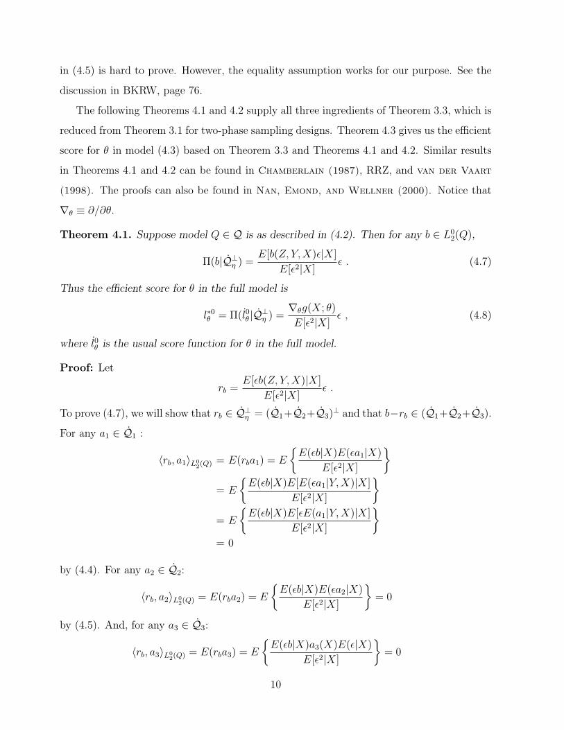
in (4.5) is hard to prove. However, the equality assumption works for our purpose. See the
discussion in BKRW, page 76.
The following Theorems 4.1 and 4.2 supply all three ingredients of Theorem 3.3, which is
reduced from Theorem 3.1 for two-phase sampling designs. Theorem 4.3 gives us the efficient
score for θ in model (4.3) based on Theorem 3.3 and Theorems 4.1 and 4.2. Similar results
in Theorems 4.1 and 4.2 can be found in Chamberlain (1987), RRZ, and van der Vaart
(1998). The proofs can also be found in Nan, Emond, and Wellner (2000). Notice that
∇θ ≡ ∂/∂θ.
Theorem 4.1. Suppose model Q ∈ Q is as described in (4.2). Then for any b ∈ L02(Q),
Π(b|Q⊥η ) =
E[b(Z, Y, X)ε|X]
E[ε2|X]ε . (4.7)
Thus the efficient score for θ in the full model is
l∗0θ = Π(l0θ |Q⊥η ) =
∇θg(X; θ)
E[ε2|X]ε , (4.8)
where l0θ is the usual score function for θ in the full model.
Proof: Let
rb =E[εb(Z, Y, X)|X]
E[ε2|X]ε .
To prove (4.7), we will show that rb ∈ Q⊥η = (Q1+Q2+Q3)
⊥ and that b−rb ∈ (Q1+Q2+Q3).
For any a1 ∈ Q1 :
〈rb, a1〉L02(Q) = E(rba1) = E
{E(εb|X)E(εa1|X)
E[ε2|X]
}
= E
{E(εb|X)E[E(εa1|Y, X)|X]
E[ε2|X]
}
= E
{E(εb|X)E[εE(a1|Y, X)|X]
E[ε2|X]
}
= 0
by (4.4). For any a2 ∈ Q2:
〈rb, a2〉L02(Q) = E(rba2) = E
{E(εb|X)E(εa2|X)
E[ε2|X]
}= 0
by (4.5). And, for any a3 ∈ Q3:
〈rb, a3〉L02(Q) = E(rba3) = E
{E(εb|X)a3(X)E(ε|X)
E[ε2|X]
}= 0
10
since E(ε|X) = 0. Hence rb ∈ Q⊥η .
Let b − rb = b − E[b|X] − rb + E[b|X]. Since E{b − E[b|X] − rb|X} = 0 and E{(b −E[b|X] − rb)ε|X} = 0, we know that b − E[b|X] − rb ∈ Q2. The other part has zero mean
since b ∈ L02(Q), so E[b|X] ∈ Q3. Thus b − rb ∈ (Q2 + Q3) ⊂ Qη, which shows the desired
result.
The efficient score l∗0θ can be obtained via direct calculation from (4.7) and using the fact
that E[−ε(f ′2/f2)(ε|X)|X] = 1. 2
Theorem 4.2. Q⊥η = {ζ(X)ε : E[ζ2(X)ε2] < ∞} .
Proof: Take a1 ∈ Q1, a2 ∈ Q2, and a3 ∈ Q3. Then we have E[a1ζ(X)ε|X] = 0,
E[a2ζ(X)ε|X] = 0, and E[a3ζ(X)ε|X] = 0, as in the proof of Theorem 4.1, which shows
{ζ(X)ε : E[ε2ζ2(X)] < ∞} ⊂ Q⊥η . Equation (4.7) shows the reverse inclusion, since
E
{E2(εb|X)
E2(ε2|X)ε2
}≤ Eb2 < ∞
by the Cauchy inequality. 2
Theorem 4.3. The efficient score l∗θ for the observed model (4.3) is given by
l∗θ =∇θg(X; θ)
E[
1πε2 − 1−π
πE2(ε|Z, X)
∣∣∣X]
{R
πY − R− π
πE[Y |Z,X]− g(X; θ)
}. (4.9)
Proof: From Theorem 3.3 and Theorem 4.2 we have
Π
(1
πζε− 1− π
πE[ζε|Z,X]
∣∣∣Q⊥η
)= l∗0θ .
Applying Theorem 4.1 we obtain:
∇θg(X; θ)
E[ε2|X]ε =
1
E[ε2|X]E
[1
πζε2 − ε
1− π
πE(ζε|Z,X)
∣∣∣X]
ε
=1
E[ε2|X]E
[1
πε2 − 1− π
πE2(ε|Z, X)
∣∣∣X]
ζε .
Simplifying the above equality yields
ζ(X) =∇θg(X; θ)
E[
1πε2 − 1−π
πE2(ε|Z,X)
∣∣∣X] .
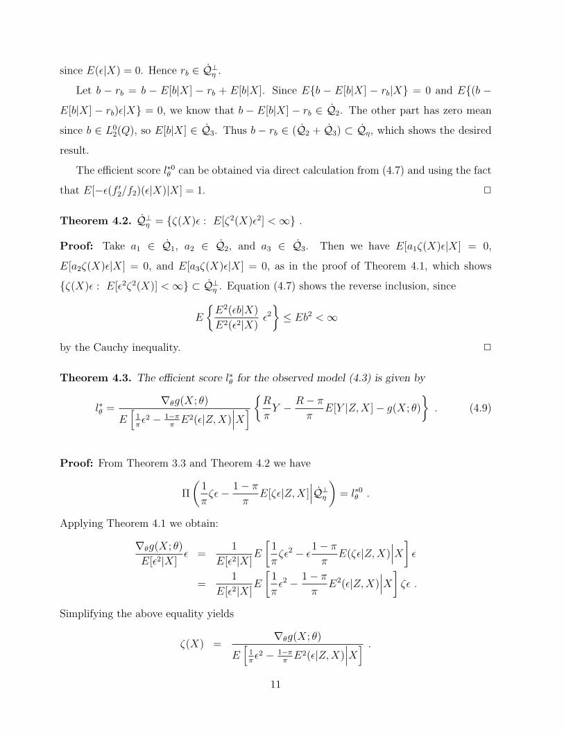
11

Thus from Theorem 3.3 we have
l∗θ =R
πζ(X)ε− R− π
πE[εζ(X)|Z, X]}
= ζ(X)
{R
πε− R− π
πE[ε|Z, X]
}
= ζ(X)
{R
πY − R− π
πE[Y |Z, X]− g(X; θ)
},
which yields (4.9). 2
Let
Y ′ =R
πY − R− π
πE[Y |Z,X] . (4.10)
Using nested conditioning, we can easily verify that E[Y ′|X] = E[Y |X] = g(X; θ) and
E[(Y ′ − g(X; θ))2|X] = E[
1πε2 − 1−π
πE2(ε|Z,X)
∣∣∣X]. Hence the efficient score l∗θ is actually
the efficient score for the “full” data (Y ′, X) applying “transformation” (4.10) to the response
variable, i.e.,
l∗θ =∇θg(X; θ)
E[ε′2|X]ε′ , (4.11)
where ε′ = Y ′ − g(X; θ). So analyzing the observed data (Z, RY,X, R) with the outcome
Y missing at random and the availability of surrogate outcome Z is actually equivalent to
analyzing the “full” data (Y ′, X) with the same conditional mean structure as that of (Y, X).
The interpretation of the parameter θ does not change at all, even though the scale of Y ′
may not be the same as Y . We refer Nan (2003) for detailed discussions of estimating θ
from equation (4.11). The proof of Theorem 4.3 is taken from the the Appendix of the same
paper.
There are many applications of the main results in Section 3 in literature. Very often in
practice the operator equation (3.2), or (3.4), or (3.6) is some kind of integral equation, so the
efficient score usually does not have a simple closed form as (4.9). The computing of efficient
estimates may have to involve solving integral equations. Among those applications, we refer
Robins, Rotnitzky, and Zhao (1995) for longitudinal studies with dropouts, Holcroft,
Rotnitzky, and Robins (1997) for multistage studies, Nan, Emond, and Wellner (2000)
for classical and mean regression models with missing covariates, and Nan, Emond, and
Wellner (2002) for Cox model with missing data.
12

5 Proofs of Main Results
5.1 Preliminaries
In this section we first introduce some preliminary results that we will use for the proofs of
main results in Section 3 and for the proofs in Section 6. All these results appeared in RRZ
and RR in a variety of ways.
For any (one-dimensional) regular parametric submodel π(R,X(R); γ) passing through
the true parameter π = π(R,X(R)) at γ = 0, we can calculate the score operator for π as
lπa = a(R, X(R)) ≡(
∂ log π(R,X(R); γ)
∂γ
)
γ=0
.
Thus Pπ = [lπa] for all a ∈ L02(P ), where [ · ] means closed linear span.
Lemma 5.1. Pπ ⊂ N (AT).
(Briefly described in the proof of Lemma 8.2 in RRZ)
Proof: For any regular parametric submodel π(R, X(R); γ) described above, we have
E[lπa |X] = E
[(∂ log π(R,X(R); γ)
∂γ
)
γ=0
∣∣∣∣∣ X
]
=∑
r
(∂ log π(r,X(r); γ)
∂γ
)
γ=0
P (R = r |X)
=∑
r
(∂π(r,X(r); γ)/∂γ
π(r, X(r); γ)
)
γ=0
π(r, X(r))
=∑
r
(∂π(r,X(r); γ)
∂γ
)
γ=0
=
(∂
∂γ
∑r
π(r,X(r); γ)
)
γ=0
= 0.
2
Remark: RRZ claimed equality of the two spaces when π is totally unspecified. We only
show the inclusion in Lemma 5.1 since this is enough for the purpose.
Lemma 5.2. The operator A is a continuous linear operator, and satisfies ‖A(g0)‖2 ≥σ‖g0‖2
0 for all g0 ∈ L02(Q). Hence A has a continuous inverse A−1.
13
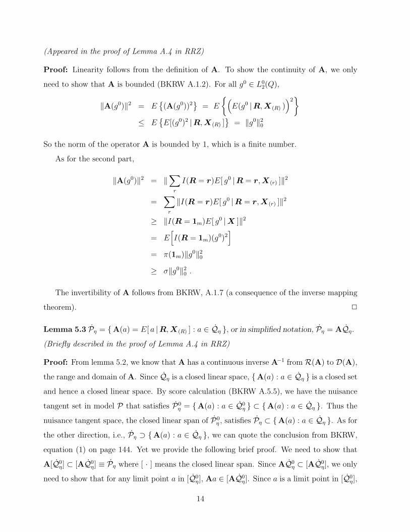
(Appeared in the proof of Lemma A.4 in RRZ)
Proof: Linearity follows from the definition of A. To show the continuity of A, we only
need to show that A is bounded (BKRW A.1.2). For all g0 ∈ L02(Q),
‖A(g0)‖2 = E{(A(g0))2
}= E
{(E(g0 |R,X(R) )
)2}
≤ E{E[(g0)2 |R, X(R) ]
}= ‖g0‖2
0
So the norm of the operator A is bounded by 1, which is a finite number.
As for the second part,
‖A(g0)‖2 = ‖∑
r
I(R = r)E[ g0 |R = r, X(r) ]‖2
=∑
r
‖I(R = r)E[ g0 |R = r, X(r) ]‖2
≥ ‖I(R = 1m)E[ g0 |X ]‖2
= E[I(R = 1m)(g0)2
]
= π(1m)‖g0‖20
≥ σ‖g0‖20 .
The invertibility of A follows from BKRW, A.1.7 (a consequence of the inverse mapping
theorem). 2
Lemma 5.3 Pη = {A(a) = E[ a |R,X(R) ] : a ∈ Qη }, or in simplified notation, Pη = AQη.
(Briefly described in the proof of Lemma A.4 in RRZ)
Proof: From lemma 5.2, we know that A has a continuous inverse A−1 from R(A) to D(A),
the range and domain of A. Since Qη is a closed linear space, {A(a) : a ∈ Qη } is a closed set
and hence a closed linear space. By score calculation (BKRW A.5.5), we have the nuisance
tangent set in model P that satisfies P0η = {A(a) : a ∈ Q0
η } ⊂ {A(a) : a ∈ Qη }. Thus the
nuisance tangent space, the closed linear span of P0η , satisfies Pη ⊂ {A(a) : a ∈ Qη }. As for
the other direction, i.e., Pη ⊃ {A(a) : a ∈ Qη }, we can quote the conclusion from BKRW,
equation (1) on page 144. Yet we provide the following brief proof. We need to show that
A[Q0η] ⊂ [AQ0
η] ≡ Pη where [ · ] means the closed linear span. Since AQ0η ⊂ [AQ0
η], we only
need to show that for any limit point a in [Q0η], Aa ∈ [AQ0
η]. Since a is a limit point in [Q0η],
14

there exists a sequence an ∈ < Q0η > such that limn an = a where < · > denotes the linear
span. By the continuity of A, we have limn Aan = Aa. Since Aan ∈ < AQ0η >, we have
Aa ∈ [AQ0η]. 2
Corollary 5.1. Pη ⊥N (AT).
(Part of Lemma A.3 in RRZ)
Proof: For all a ∈ N (AT) and all g0 ∈ Qη, it is easy to see that 〈A(g0), a 〉 =
〈 g0, AT(a) 〉0 = 〈 g0, 0 〉0 = 0. We obtain the conclusion from Lemma 5.3. 2
From Lemma 5.1 and Corollary 5.1 we know that Pπ and Pη are orthogonal, so we can
write the nuisance tangent space for model P as the following:
Corollary 5.2. Pη,π = Pη + Pπ.
(Part of Lemma A.3 in RRZ)
Corollary 5.3 Let g ∈ L02(P ). Then g ∈ P⊥η if and only if ATg ∈ Q⊥
η .
(Lemma A.6 in RRZ)
Proof: This is obvious since Pη = AQη from Lemma 5.3 and for any h0 ∈ Qη, 〈ATg, h0 〉0 =
〈 g, Ah0 〉 = 0. 2
Lemma 5.4 Operator ATA is invertible.
(Appeared in the proof of Proposition 8.1 part d in RRZ)
Proof: Write ATA = I − [I −ATA], where I is the identity operator. To see that ATA is
invertible, we need only to show that ‖I−ATA‖0 < 1.
‖I−ATA‖20 = sup
‖g0‖=1
〈 [I−ATA](g0) , [I−ATA](g0) 〉0
= sup‖g0‖=1
〈 g0 , [I−ATA](g0) 〉0
= 1− inf‖g0‖=1
〈 g0 , ATA(g0) 〉0= 1− inf
‖g0‖=1〈A(g0) , A(g0) 〉
≤ 1− inf‖g0‖=1
σ‖g0‖20
< 1− σ ,
15
where the second equality holds because I −ATA is self-adjoint (see e.g. Conway (1990),
Proposition 2.13 on page 34). 2
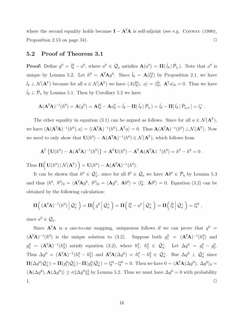
5.2 Proof of Theorem 3.1
Proof: Define g0 = l0θ − a0, where a0 ∈ Qη satisfies A(a0) = Π( lθ | Pη ). Note that a0 is
unique by Lemma 5.2. Let h0 = ATAg0. Since lθ = A(l 0θ ) by Proposition 2.1, we have
lθ ⊥ N (AT) because for all a ∈ N (AT) we have 〈A(l0θ), a〉 = 〈l0θ , ATa〉0 = 0. Thus we have
lθ ⊥ Pπ by Lemma 5.1. Then by Corollary 5.2 we have
A(ATA)−1(h0) = A(g0) = Al0θ −Aa0θ = lθ −Π( lθ | Pη ) = lθ −Π[ lθ | Pη,π ] = l ∗θ .
The other equality in equation (3.1) can be argued as follows. Since for all a ∈ N (AT),
we have 〈A(ATA)−1(h0), a〉 = 〈(ATA)−1(h0),ATa〉 = 0. Thus A(ATA)−1(h0)⊥N (AT). Now
we need to only show that U(h0)−A(ATA)−1(h0) ∈ N (AT), which follows from
AT{U(h0)−A(ATA)−1(h0)
}= ATU(h0)−ATA(ATA)−1(h0) = h0 − h0 = 0 .
Thus Π(
U(h0) | N (AT))
= U(h0)−A(ATA)−1(h0).
It can be shown that h0 ∈ Q⊥η , since for all b0 ∈ Qη we have Ab0 ∈ Pη by Lemma 5.3
and thus 〈h0, b0〉0 = 〈ATAg0, b0〉0 = 〈Ag0, Ab0〉 = 〈l∗θ , Ab0〉 = 0. Equation (3.2) can be
obtained by the following calculation:
Π(
(ATA)−1(h0)∣∣∣ Q⊥
η
)= Π
(g0
∣∣∣ Q⊥η
)= Π
(l0θ − a0
∣∣∣ Q⊥η
)= Π
(l0θ
∣∣∣ Q⊥η
)= l∗0θ ,
since a0 ∈ Qη.
Since ATA is a one-to-one mapping, uniqueness follows if we can prove that g0 =
(ATA)−1(h0) is the unique solution to (3.2). Suppose both g01 = (ATA)−1(h0
1) and
g02 = (ATA)−1(h0
2) satisfy equation (3.2), where h01, h0
2 ∈ Q⊥η . Let ∆g0 = g0
1 − g02.
Thus ∆g0 = (ATA)−1(h01 − h0
2) and ATA(∆g0) = h01 − h0
2 ∈ Q⊥η . But ∆g0 ⊥ Q⊥
η since
Π(∆g0|Q⊥η ) = Π(g0
1|Q⊥η )−Π(g0
2|Q⊥η ) = l∗0θ −l∗0θ = 0. Then we have 0 = 〈ATA(∆g0), ∆g0〉0 =
〈A(∆g0),A(∆g0)〉 ≥ σ‖∆g0‖20 by Lemma 5.2. Thus we must have ∆g0 = 0 with probability
1. 2
16

5.3 Proof of Theorem 3.2
The proof of Theorem 3.2 will involve a lot of algebra for the π’s defined in Subsection 3.2.
From the MAR assumption in (2.1) we have
P (Rk = 1 |X) = 1−∑
j<k
P (R = 1j |X)
= 1−∑
j<k
P (R = 1j |X(1k−1))
= P (Rk = 1 |X(1k−1)) . (5.1)
Hence,
P (Rk = 1 |Rk−1 = 1,X) =P (Rk = 1 |X)
P (Rk−1 = 1 |X)
=P (Rk = 1 |X(1k−1))
P (Rk−1 = 1 |X(1k−1))
= πk , (5.2)
and
P (Rk+t = 1 |Rk−1 = 1, X) = P (Rk+t = 1, Rk+t−1 = 1, · · · , Rk = 1 |Rk−1 = 1, X)
= P (Rk+t = 1 |Rk+t−1 = 1, X) · · ·P (Rk = 1 |Rk−1 = 1,X)
= πk+t · · · πk
=πk+t
πk−1
. (5.3)
From (5.2) we also have
P (Rk = 1 |X) = πkP (Rk−1 = 1 |X) = πk . (5.4)
Thus for j < m we obtain
π(1j) = P (Rj+1 = 0, Rj = 1 |X)
= P (Rj+1 = 0 |Rj = 1,X)P (Rj = 1 |X)
= (1− πj+1)πj
= πj − πj+1 . (5.5)
17

Now we show the following two additional identities that we will apply to the proofs in
this subsection.
Lemma 5.5. For any l ≤ m,
l∑
k=1
1− πk
πk
+ 1 =1
πl
.
Proof: When l = 1, we have
l∑
k=1
1− πk
πk
+ 1− 1
πl
=1− π1
π1
+ 1− 1
π1
= 0 .
When l > 1, we have
l∑
k=1
1− πk
πk
+ 1− 1
πl
=l−1∑
k=1
1− πk
πk
+ 1− 1
πl−1
= · · ·
=1∑
k=1
1− πk
πk
+ 1− 1
π1
=1− π1
π1
+ 1− 1
π1
= 0 .
2
Corollary 5.4 For any 1 ≤ l ≤ m,
m∑
k=l
1− πk
πk
=1
πm
− 1
πl−1
.
Proof: By Lemma 5.5, we have
m∑
k=l
1− πk
πk
=m∑
k=1
1− πk
πk
−l−1∑
k=1
1− πk
πk
=
(1
πm
− 1
)−
(1
πl−1
− 1
)=
1
πm
− 1
πl−1
.
2
Theorem 3.2 is a direct consequence of Theorem 3.1 once we obtain the following
calculations that are based on Proposition 8.2 in RRZ. We use Lemma 5.5 and Corollary 5.4
several times without referring in the proof of the following Proposition 5.1.
Proposition 5.1 For monotonic missingness we have
18
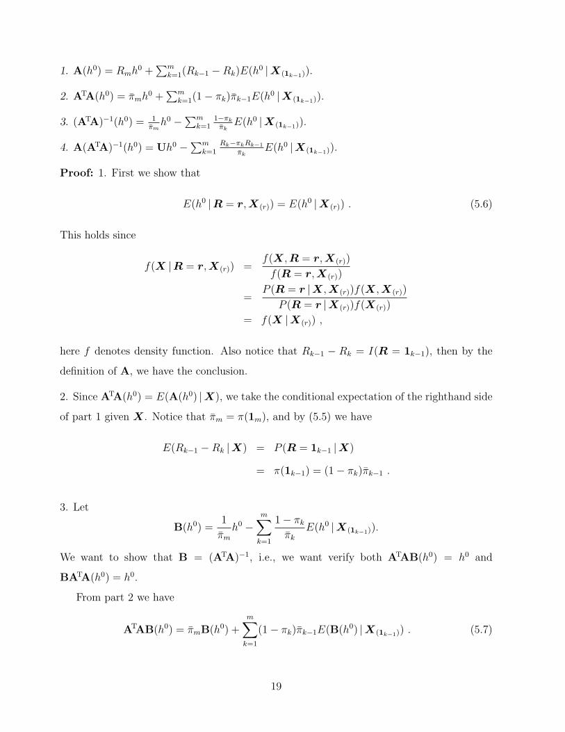
1. A(h0) = Rmh0 +∑m
k=1(Rk−1 −Rk)E(h0 |X(1k−1)).
2. ATA(h0) = πmh0 +∑m
k=1(1− πk)πk−1E(h0 |X(1k−1)).
3. (ATA)−1(h0) = 1πm
h0 −∑mk=1
1−πk
πkE(h0 |X(1k−1)).
4. A(ATA)−1(h0) = Uh0 −∑mk=1
Rk−πkRk−1
πkE(h0 |X(1k−1)).
Proof: 1. First we show that
E(h0 |R = r,X(r)) = E(h0 |X(r)) . (5.6)
This holds since
f(X |R = r,X(r)) =f(X,R = r,X(r))
f(R = r, X(r))
=P (R = r |X, X(r))f(X, X(r))
P (R = r |X(r))f(X(r))
= f(X |X(r)) ,
here f denotes density function. Also notice that Rk−1 − Rk = I(R = 1k−1), then by the
definition of A, we have the conclusion.
2. Since ATA(h0) = E(A(h0) |X), we take the conditional expectation of the righthand side
of part 1 given X. Notice that πm = π(1m), and by (5.5) we have
E(Rk−1 −Rk |X) = P (R = 1k−1 |X)
= π(1k−1) = (1− πk)πk−1 .
3. Let
B(h0) =1
πm
h0 −m∑
k=1
1− πk
πk
E(h0 |X(1k−1)).
We want to show that B = (ATA)−1, i.e., we want verify both ATAB(h0) = h0 and
BATA(h0) = h0.
From part 2 we have
ATAB(h0) = πmB(h0) +m∑
k=1
(1− πk)πk−1E(B(h0) |X(1k−1)) . (5.7)
19

By the above definition of B, the first term of RHS of (5.7) can be written as
πmB(h0) = h0 −m∑
k=1
πm(1− πk)
πk
E(h0 |X(1k−1)) , (5.8)
and the second term is
m∑
k=1
(1− πk)πk−1E(B(h0) |X(1k−1))
=m∑
k=1
(1− πk)πk−1E(h0/πm |X(1k−1))
−m∑
k=1
(1− πk)πk−1E
[m∑
j=1
(1− πj)π−1j {E(h0 |X1j−1
)}∣∣∣∣∣ X(1k−1)
]
=m∑
k=1
(1− πk)πk−1E(h0/πm |X(1k−1))−m∑
k=1
(1− πk)πk−1
{ k∑j=1
(1− πj)π−1j E(h0 |X1j−1
)}
−m∑
k=1
(1− πk)πk−1E
[m∑
j=k+1
(1− πj)π−1j h0
∣∣∣∣∣ X(1k−1)
]
=m∑
k=1
(1− πk)πk−1E(h0/πm |X(1k−1))−m∑
k=1
k∑j=1
(1− πk)πk−1(1− πj)π−1j E(h0 |X1j−1
)
−m∑
k=1
(1− πk)πk−1E
[( 1
πm
− 1
πk
)h0
∣∣∣∣ X(1k−1)
]
= −m∑
j=1
(1− πj)π−1j E(h0 |X1j−1
){ m∑
k=j
(1− πk)πk−1
}
+m∑
k=1
(1− πk)πk−1E
[1
πk
h0
∣∣∣∣ X(1k−1)
]
= −m∑
j=1
(1− πj)π−1j E(h0 |X1j−1
)(πj−1 − πm
)+
m∑
k=1
(1− πk)πk−1E
[1
πk
h0
∣∣∣∣ X(1k−1)
]
= −m∑
j=1
(1− πj)πj−1π−1j E(h0 |X1j−1
) +m∑
j=1
πm(1− πj)π−1j E(h0 |X1j−1
)
+m∑
k=1
(1− πk)πk−1π−1k E
[h0
∣∣ X(1k−1)
]
=m∑
j=1
πm(1− πj)π−1j E(h0 |X1j−1
) . (5.9)
Now combine (5.8) and (5.9) into (5.7), we have ATAB(h0) = h0.
20
By the definition of B we have
BATA(h0) = ATA(h0)/πm −m∑
k=1
(1− πk)π−1k E(ATA(h0) |X(1k−1)) . (5.10)
From part 2, the first term of RHS of (5.10) is
ATA(h0)/πm = h0 +m∑
k=1
(1− πk)πk−1π−1m E(h0 |X(1k−1)) , (5.11)
and the second term, without the minus sign, is
m∑
k=1
(1− πk)π−1k E(ATA(h0) |X(1k−1))
=m∑
k=1
(1− πk)π−1k E
[πmh0 +
m∑j=1
(1− πj)πj−1E(h0 |X1j−1)
∣∣∣∣∣ X(1k−1)
]
=m∑
k=1
(1− πk)π−1k E(πmh0 |X(1k−1)) +
m∑
k=1
(1− πk)π−1k
{k∑
j=1
(1− πj)πj−1E(h0 |X1j−1)
}
+m∑
k=1
(1− πk)π−1k
{E
[m∑
j=k+1
(1− πj)πj−1h0
∣∣∣∣∣ X(1k−1)
]}
=m∑
k=1
(1− πk)π−1k E(πmh0 |X(1k−1)) +
m∑
k=1
k∑j=1
(1− πk)π−1k (1− πj)πj−1E(h0 |X1j−1
)
+m∑
k=1
(1− πk)π−1k
{E
[(πk − πm
)h0
∣∣∣ X(1k−1)
]}
=m∑
j=1
(1− πj)πj−1E(h0 |X1j−1)
{m∑
k=j
(1− πk)π−1k
}
+m∑
k=1
(1− πk)π−1k E
[πkh
0 |X(1k−1)
]
=m∑
j=1
(1− πj)πj−1E(h0 |X1j−1)
{1
πm
− 1
πj−1
}+
m∑
k=1
(1− πk)π−1k E
[πkh
0 |X(1k−1)
]
=m∑
j=1
(1− πj)πj−1π−1m E(h0 |X1j−1
)−m∑
j=1
(1− πj)E(h0 |X1j−1)
+m∑
k=1
(1− πk)E[h0 |X(1k−1)
]
=m∑
j=1
(1− πj)πj−1π−1m E(h0 |X1j−1
) . (5.12)
21
Now combine (5.11) and (5.12) into (5.10), we have BATA(h0) = h0.
4. From part 1 we have
A(ATA)−1(h0) = Rm(ATA)−1(h0) +m∑
k=1
(Rk−1 −Rk)E((ATA)−1(h0) |X(1k−1)) . (5.13)
From part 3, the first term of RHS of (5.13) can be written as
Rm(ATA)−1(h0) = Rmh0/πm −m∑
k=1
Rm(1− πk)π−1k E(h0 |X(1k−1)) , (5.14)
and the second term ism∑
k=1
(Rk−1 −Rk)E((ATA)−1(h0) |X(1k−1))
=m∑
k=1
(Rk−1 −Rk)E
{h0/πm −
m∑j=1
(1− πj)π−1j E(h0 |X1j−1
)
∣∣∣∣∣ X(1k−1)
}
=m∑
k=1
(Rk−1 −Rk)E{
h0/πm
∣∣ X(1k−1)
}
−m∑
k=1
(Rk−1 −Rk)E
{m∑
j=1
(1− πj)π−1j E(h0 |X1j−1
)
∣∣∣∣∣ X(1k−1)
}
=m∑
k=1
(Rk−1 −Rk)E{
h0/πm
∣∣ X(1k−1)
}−m∑
k=1
(Rk−1 −Rk)
{k∑
j=1
(1− πj)π−1j E(h0 |X1j−1
)
}
−m∑
k=1
(Rk−1 −Rk)E
{m∑
j=k+1
(1− πj)π−1j h0
∣∣∣∣∣ X(1k−1)
}
=m∑
k=1
(Rk−1 −Rk)E{
h0/πm
∣∣ X(1k−1)
}−m∑
k=1
k∑j=1
(Rk−1 −Rk)(1− πj)π−1j E(h0 |X1j−1
)
−m∑
k=1
(Rk−1 −Rk)E
[ ( 1
πm
− 1
πk
)h0
∣∣∣∣ X(1k−1)
]
=m∑
k=1
(Rk−1 −Rk)E{
h0/πm
∣∣ X(1k−1)
}−m∑
j=1
(1− πj)π−1j E(h0 |X1j−1
)
[m∑
k=j
(Rk−1 −Rk)
]
−m∑
k=1
(Rk−1 −Rk)E[
h0/πm
∣∣ X(1k−1)
]+
m∑
k=1
(Rk−1 −Rk)E[
h0/πk
∣∣ X(1k−1)
]
= −m∑
j=1
(1− πj)π−1j E(h0 |X1j−1
)(Rj−1 −Rm)
+m∑
k=1
(Rk−1 −Rk)E[
h0/πk
∣∣ X(1k−1)
]. (5.15)
22

Now combine (5.14) and (5.15) into (5.13), we have
A(ATA)−1(h0) = Rmh0/πm +m∑
k=1
{−Rm(1− πk)π
−1k − (1− πk)π
−1k (Rk−1 −Rm)
+(Rk−1 −Rk)π−1k
}E(h0 |X(1k−1))
= Rmh0/πm +m∑
k=1
{−Rm(1− πk)− (1− πk)Rk−1
+(1− πk)Rm + (Rk−1 −Rk)}
π−1k E(h0 |X(1k−1))
= Rmh0/πm +m∑
k=1
{πkRk−1 −Rk
}π−1
k E(h0 |X(1k−1))
= Uh0 −m∑
k=1
Rk − πkRk−1
πk
E(h0 |X(1k−1)) .
2
Proof of Theorem 3.2: Theorem 3.2 follows directly from Theorem 3.1 using the results
in Proposition 5.1 part 3 and part 4. 2
5.4 Proof of Theorem 3.3
Proof: Since for two-phase designs we have
Rk =
{1, if k ≤ tRm, if k ≥ t + 1,
(5.16)
and
πk =
{1, if k 6= t + 1π(1m), if k = t + 1,
(5.17)
then by Proposition 5.1 part 3 and (5.17) we obtain
(ATA)−1(h0) = h0/πm − (1− πt+1)π−1t+1E(h0 |X(1t)) =
1
π(1m)h0 − 1− π(1m)
π(1m)E(h0 |X(1t)) ,
and by Proposition 5.1 part 4, (5.16) and (5.17),
A(ATA)−1(h0) = Uh0 −m∑
k=1
(Rk − πkRk−1
)π−1
k E(h0 |X(1k−1))
= Uh0 −∑
k 6=t+1
Rk −Rk−1
πk
E(h0 |X(1k−1)) +Rt+1 − π(1m)Rt
πt+1
E(h0 |X(1t))
23

= Uh0 − Rm − π(1m)
π(1m)E(h0 |X(1t))
=I(R = 1m)
π(1m)h0 − I(R = 1m)− π(1m)
π(1m)E(h0 |X(1t)).
Then applying Theorem 3.1 or Theorem 3.2 we obtain Theorem 3.3.
Another way of reducing the results of monotonic missingness (Theorem 3.2) to that of
two-phase sampling design is to view the first t components of X as the first variable and
the rest as the second. Then we have m = 2 and the first variable is always observable.
Hence R1 = 1 and π1 = 1, and the reduction is obvious. 2
6 Space of Influence Functions / Estimating Functions
Since finding efficient estimates can be very challenging for missing data problems, we may
be interested in some inefficient estimators that are relatively easy to compute and have
satisfactory efficiency. As we know from BKRW, the space of all influence functions (or
estimating functions) for regular asymptotically linear estimators of θ in model P is a subset
of P⊥η,π. Hence characterizing the space P⊥η,π becomes important.
Since the influence function ψ for any regular asymptotically linear estimator has the
property that ψ⊥Pη,π and 〈ψ, lθ〉 = 1, we have the following representation of the space of
influence functions:
Lemma 6.1.
1. Ψθ = {〈 g, lθ 〉−1g : g ∈ P⊥η,π} = {g ∈ P⊥η,π : 〈g, lθ 〉 = 1} ⊂ P⊥η,π
2. Ψ0θ = {〈 g0, l 0
θ 〉−10 g0 : g0 ∈ Q⊥
η } = {g0 ∈ Q⊥η : 〈g0, l 0
θ 〉0 = 1} ⊂ Q⊥η
3. For any g ∈ P⊥η,π, 〈 g, l ∗θ 〉 = 〈 g, lθ 〉.
(Lemma 8.1 in RRZ)
Proof: The proof is trivial and thus omitted.
The following Propositions 6.1-6.3 can be found from Proposition 8.1 in RRZ.
Proposition 6.1. For any g ∈ P⊥η,π, it can be decomposed as
g = U(ATg) +(g −U(ATg)
),
24

where ATg ∈ Q⊥η and g −U(ATg) ∈ N (AT).
Proof: Since g ∈ P⊥η,π ⊂ P⊥η , we have ATg ∈ Q⊥η by Corollary 5.3. The other part can be
shown by
AT(g −U{ATg}
)= ATg −ATg = 0
using the fact in Proposition 2.1, part 2. 2
Proposition 6.2. P⊥η,π = {V(g0, a) : g0 ∈ Q⊥η , a ∈ N (AT)}
Proof: We first prove P⊥η,π ⊃ {V(g0, a) : g0 ∈ Q⊥η , a ∈ N (AT)}. By the definition of V, we
know that V(g0, a) ∈ P⊥π . From Corollary 5.2 we have Pη,π = Pη + Pπ, so we need to only
show that V(g0, a) ∈ P⊥η , i.e., 〈V(g0, a),A(h0) 〉 = 0 for all h0 ∈ Qη. For any a ∈ N (AT)),
by Lemma 5.1 we have
ATV(g0, a) = ATU(g0) + AT{
a−Π(
U(g0) + a∣∣∣ Pπ
)}= ATU(g0) + 0 = g0.
Thus 〈V(g0, a), A(h0) 〉 = 〈ATV(g0, a), h0 〉0 = 〈 g0, h0 〉0 = 0 since g0 ∈ Q⊥η and h0 ∈ Qη.
Now we show P⊥η,π ⊂ {V(g0, a) : g0 ∈ Q⊥η , a ∈ N (AT)}, i.e., for any g ∈ P⊥η,π, we want
to find some g0 ∈ Q⊥η and a ∈ N (AT) such that g = V(g0, a). This is obviously true from
Proposition 6.1 and g⊥Pπ. 2
Remark: The above Proposition 6.2 characterizes the space P⊥η,π, which contains all the
estimating functions (or influence functions) for regular asymptotically linear estimators in
model P . From the definition of operator V in Definition 2.1 we see that any estimating
function in model P is an inverse probability weighted estimating function in model Q plus a
term which has expectation zero given full data X. This property gives us great opportunity
and flexibility to develop estimating methods for missing data problems if we have enough
knowledge about the complete data model. It can be easily shown that for a two-phase
sampling design where π is given, the second term in any estimating function has the form
−(Rm − π(1m))π(1m)−1φ(X(1t)), where φ has finite second moment.
Proposition 6.3. If g0 ∈ Q⊥η and a ∈ N (AT), then 〈V(g0, a), l ∗θ 〉 = 〈 g0, l∗0θ 〉0.
Proof: By Lemma 6.1 part 3 and Proposition 6.2, we have 〈V(g0, a), l ∗θ 〉 = 〈V(g0, a), lθ〉 =
〈V(g0, a), Al 0θ 〉 = 〈ATV(g0, a), l 0
θ 〉0 = 〈g0, l 0θ 〉0 = 〈g0, l∗0θ 〉0 . 2
25
The following two propositions are properties for spaces of influence functions.
Proposition 6.4. If g ∈ Ψθ, then ATg ∈ Ψ0θ.
Proof: For any g ∈ Ψθ, we have g ∈ P⊥η,π ⊂ P⊥η , and thus ATg ∈ Q⊥η with 〈ATg, l 0
θ 〉0 =
〈g, Al 0θ 〉 = 〈g, lθ〉 = 1. 2
Proposition 6.5. Ψθ = {V(g0, a) : g0 ∈ Ψ0θ, a ∈ N (AT)} = { 〈g0, l∗0θ 〉−1
0 V(g0, a) : g0 ∈Q⊥
η , a ∈ N (AT) }.
Proof: By Lemma 6.1 and Proposition 6.2, we need to only show for the first equality that
〈V(g0, a), lθ〉 = 1 for g0 ∈ Ψ0θ, a ∈ N (AT), which is easily seen from Proposition 6.3, i.e.,
〈V(g0, a), l ∗θ 〉 = 〈g0, l∗0θ 〉0 = 1 for g0 ∈ Ψ0θ. The second equality can be verified directly by
using Proposition 6.3 and Lemma 6.1 part 1. 2
7 Discussion
The major challenges in deriving efficient score functions for models with missing data can
be the characterization of space Q⊥η and the calculation of the projection onto this space.
Although these problems have been successfully solved for the models discussed in the papers
cited at the end of Section 4, there are still many unsolved problems for other complicated
models. Even though sometime we are able to obtain the efficient score function, finding
efficient estimates can also be very challenging. We refer Nan (2002) for an example on
this line. It is not unusual that we compromise efficiency (or make stronger assumptions) to
obtain certain computable estimates. Thus the characterization of space P⊥η,π in Proposition
6.2 can be very helpful.
Acknowledgements
The authors would like to thank Mary Emond and Jon Wellner for their generous help in
this research.
Appendix
Table 1 lists the two sets of corresponding notation used in RRZ and our paper.
26

References
Bickel P. J. , Klaassen C. A. J., Ritov Y and Wellner J. A. (1993). Efficient and adaptive
inference in semiparametric models. Johns Hopkins University Press, Baltimore.
Chamberlain G. (1987). Asymptotic Efficiency in Estimation With Conditional Moment
Restrictions, Journal of Econometrics, 34, 305-324.
Conway J. B. (1990). A Course in Functional Analysis. Springer-Verlag, New York.
Holcroft, C. A., Rotnitzky, A. and Robins, J. M. (1997) Efficient estimation of regression
parameters from multistage studies with validation of outcome and covariates. Journal
of Statistical Planning and Inference, 65, 349-374.
Horvitz, D. G. and Thompson, D. J. (1952). A generalization of sampling without
replacement from a finite universe. Journal of the American Statistical Association,
47, 663-685.
Little, R. J. A. and Rubin, D. (1987). Statistical Analysis with Missing Data. John Wiley,
New York.
Nan B., Emond M. and Wellner J. A. (2000). Information bounds for regression models
with missing Data. Technical Report 378 , Department of Statistics, University of
Washington.
Nan B. (2002). Efficient estimation for case-cohort studies. Submitted.
Nan, B., Emond, M. and Wellner, J. A. (2002). Information bounds for Cox regression
models with missing data. The Annals of Statistics, to be published.
Nan B. (2003). New estimating methods for surrogate outcome data. Submitted.
Pepe, M. S. (1992). Inference using surrogate outcome data and a validation sample.
Biometrika, 79, 355-365.
Robins J. M. and Rotnitzky A. (1992). Recovery of information and adjustment for
dependent censoring using surrogate markers. AIDS Epidemiology - Methodological
Issues, 297-331. Eds. Jewell N., Dietz K., and Farewell V. Birkhauser, Boston.
27

Robins J. M. , Rotnitzky A. and Zhao L. P. (1994). Estimation of regression coefficients
when some regressors are not always observed. Journal of the American Statistical
Association, 89, 846-866.
Robins J. M. , Rotnitzky A. and Zhao L. P. (1995), Analysis of Semiparametric Regression
Model for Repeated Outcomes in the Presence of Missing Data. Journal of the
American Statistical Association, 90, 106-121.
van der Vaart, A. W. (1998). Asymptotic Statistics. Cambridge: Cambridge University
Press.
University of MichiganDepartment of Biostatistics1420 Washington HeightsAnn Arbor, MI 48109-2029U.S.A.e-mail: [email protected]
University of MichiganDepartment of Biostatistics1420 Washington HeightsAnn Arbor, MI 48109-2029U.S.A.e-mail: [email protected]
28

Table 1: Corresponding notation in our paper and RRZ.
Meaning Our Paper RRZ
Full data model
Nuisance tangent space Qη ΛF
Orthogonal complement to thenuisance tangent space
Q⊥η ΛF,⊥
0
Score for θ l 0θ SF
θ
Efficient Score for θ l∗0θ SFeff
The space of influence function Ψ0θ ΛF,⊥
0∗
Observed data model
Nuisance tangent space Pη,π Λ
Orthogonal complement to thenuisance tangent space
P⊥η,π Λ⊥0
Nuisance tangent space for π Pπ Λ(3)
Score for θ lθ Sθ
Efficient Score for θ l ∗θ Seff
The space of influence function Ψθ Λ⊥0∗
The null space of AT N (AT) Λ(2)
Operators
A g
U u
V v
ATA m
29