Cox Regression With Covariates Missing Not At Random

Victoria J. Cook1, X. Joan Hu2 and Tim B. Swartz2

1BC Centre for Disease Control and University of British Columbia

2Simon Fraser University

Abstract

This paper considers estimation under the Cox proportional hazards model with right-

censored event times in the presence of covariates missing not at random (MNAR). We

propose an approach derived from likelihood estimation utilizing supplementary informa-

tion. We show that available additional information not only helps to account appropriately

for the missing covariates but also leads to estimation procedures which are natural and easy

to implement. A medical example is used throughout the paper to motivate the problem

and to illustrate the proposed methodology.

Key words: event time; missing data; semiparametric estimation; sensitivity analysis; sup-

plementary information.

1 Introduction

In many practical studies, the observation of an event time is subject to right-censoring

and measurements on certain components of the covariates are not available on all study

subjects. It is often of interest to estimate the parameters in the Cox proportional hazards

model with such missing data. To avoid the computational burden induced by the unspeci-

fied baseline function in the model, many attempts to tackle the problem employ variations

1

of the partial likelihood estimating functions based on the right-censored event times with

complete covariate observations. See, for example, Lin and Ying (1993), Zhou and Pepe

(1995), Paik and Tsai (1997) and Qi, Wang and Prentice (2005). Notable exceptions include

Chen and Little (1999) and Herring and Ibrahim (2001), which specify parametrically the

distribution of the covariate and propose likelihood based estimation procedures. Although

there has been some excellent work on data missing not at random (MNAR) (e.g., Scharf-

stein, Rotnitzky and Robins, 1999), most published papers in this area assume that the

missing covariates are either missing completely at random (MCAR) or missing at random

(MAR).

Tuberculosis (TB) is an infectious disease spread by the airborne route. There are many

risk factors that increase a person’s chance of being infected or going on to develop active

disease. HIV infection is the single greatest risk factor associated with TB. Motivated by

a research question at the Division of TB Control, Centre for Disease Control of British

Columbia (BCCDC), we consider Cox regression with covariates missing not at random

(MNAR). An investigation was conducted to evaluate the association of the time to TB

and latent TB infection (LTBI) with a list of potential risk factors based on subjects in the

Greater Vancouver area who had contact with active infectious TB patients (i.e., source

cases); see Cook, et al (2005). A total of 7, 921 people were identified as contacts from the

TB registry and were taken as study subjects. The time to TB development of each TB

contact was collected up to October 2003. This, together with the staggered study entries,

resulted in the observation of the event times (i.e., times to TB since the contacts) subject to

a noninformative right-censoring. Excluding HIV status, information on all of the potential

risk factors was available from 97.9% of the study subjects (7, 754 out of 7, 921). With

2

respect to the HIV status covariate, only 2.2% of the study subjects (176 out of 7, 921)

had HIV test results documented in the TB registry. This lack of complete data resulted

from the data collection process due to a TB policy, which is to test all active TB cases

for HIV co-infection but not all TB contacts. However, nurses interviewed the TB contacts

and requested HIV testing in those contacts with risk factors of HIV infection. Thus the

missingness of a subject’s HIV status could be closely associated with the presented lack

of risks for HIV infection. In other words, the missingness of the covariate likely depends

on the covariate measurement. This type of missingness is also referred to as nonmissing

at random (NMAR) in the literature (c.f., Tsiatis, 2006). The well-established inverse

probability weighted complete-case estimator (Robins, Rotnitzky and Zhao, 1994) and its

extensions, augmented inverse probability weighted complete-case estimators (c.f., Bang

and Robins, 2005), are not directly applicable in handling the current missing data, and

neither is the commonly-used multiple imputation approach (c.f., Little and Rubin, 2002).

Attempts were made to adapt the conventional approach under the Cox proportional

hazards model for right-censored survival times when the covariates are fully observed. They

included focusing on the data of the complete cases, having the indicator of missingness as

an additional covariate in the analysis, and imputing all the missing HIV entries as negative.

None of these approaches appeared plausible or produced satisfactory analysis outcomes as

they would lead to either an obviously over or under estimation of the population HIV

status in the TB contacts. As pointed out in Tsiatis (2006), analysis of data with MNAR

missingness is in general problematic, since the missingness may depend on unobserved data

and adjustments for the missing data cannot be verified with the available data. These

considerations led us to explore the problem utilizing additional information.

3

In many practical situations, there is supplementary information on the covariate com-

ponents whose values associated with a portion of the study subjects are missing. This

type of information is readily available in some studies. For example, the TB contact study

team collected the prevalence information of HIV infection in different cohorts, such as

various groups of TB contacts and the general population in the Great Vancouver area

(or, in British Columbia). Other studies conducted a follow-up survey on the individuals

who had missing covariate measurements; see Suzuki (1985) for an example of this with

car warranty data. Hu and Lawless (1996, 1997) present parametric estimation approaches

based on right-censored failure times with several types of supplementary information on

the missing censoring times. In the present work, we extend their methods to a semipara-

metric setting with MNAR covariates. We assume that the time to an event of interest T

follows the Cox proportional hazards model, and present estimation procedures built upon

the likelihood function from right-censored event times with MNAR covariates in combina-

tion with additional information on the missing covariates from another source. Procedures

associated with supplementary information in different forms are developed for computing

the estimators of the regression parameters and the unspecified baseline function. They are

easy to follow and implement.

The rest of the paper is organized as follows. Section 2 introduces the framework of

the proposed approach. Sections 3 and 4 describe procedures for estimating the regression

parameters in the Cox model with the available data in combination with certain supplemen-

tary information. Section 5 reports the preliminary analyses of missing HIV status in TB

contacts, and analyzes the TB contact data augmented with HIV prevalence information.

It also presents sensitivity analyses conducted to verify adjustments for the missingness of

4

HIV entries. Some final remarks are given in Section 6.

2 Notation, Modelling and Assumptions

We formulate the aforementioned problem as follows. Suppose that an event time T con-

ditional on covariates (X,Z) follows the Cox proportional hazards model (Cox, 1972): its

conditional hazard function is

h(t|X,Z) = h0(t) exp(α′

X + β′

Z), t > 0. (2.1)

Let {(Ti,Xi, Zi) : i = 1, . . . , n} be i.i.d. realizations of (T,X,Z), associated with a study

with n individuals, where Z and X denote the covariate components with and without

entries from all the individuals, respectively. Our primary interest is in estimating the

regression coefficients α and β in the Cox model (1) from the study’s available data:

{(Ui,∆i, RiXi, Ri, Zi) : i = 1, . . . , n}, (2.2)

where Ui = Ti

∧Ci is the minimum of Ti and Ci with Ci the censoring time of subject i,

the variable ∆i indicates Ti ≤ Ci or not, and Ri is the missing indicator for whether Xi

is observed. We focus on the situations where the MAR (missing at random) assumption,

P (R|U,∆,X,Z) = P (R|U,∆, Z), does not necessarily hold, such as the TB contact study

described in Section 1.

We make the following two assumptions throughout the paper, which are plausible in

many practical situations:

A1. The censoring is conditionally noninformative: T ⊥ C | (X,Z).

5

A2. Conditional on (X,Z), (U,∆) is independent of whetherX is observed or not: P (U,∆|X,Z,R) =

P (U,∆|X,Z).

Using the generic notation for densities, the information contributed by the available data

of an individual under assumptions A1 and A2 is

[U,∆ | X,Z][X | R = 1, Z][R = 1, Z]

when R = 1;∫

[U,∆ | X,Z]d[X | R = 0, Z][R = 0, Z],

when R = 0. Further, denote the distribution function of X given R and Z = z by

GR(· | z), i.e., GR(x | z) = P (X ≤ x | R,Z = z). The distribution of X given Z = z is

then G(x | z) = p(z)G1(x | z) + (1 − p(z))G0(x | z), where p(z) = P (R = 1 | Z = z). Here

G1(· | z) and G0(· | z) are the conditional distributions of the observed X and unobserved

X given Z = z, respectively. The likelihood function based on the available data (2) is

proportional to

LF (α, β, h0, G0, G1, p) =n∏

i=1

{h(Ti|Xi, Zi)

∆iS(Ui|Xi, Zi)g1(Xi | Zi)p(Zi)}Ri

×{ ∫

h(Ti|x,Zi)∆iS(Ui|x,Zi)dG0(x | Zi)(1− p(Zi))

}1−Ri

, (2.3)

where the conditional survivor function S(t|x, z) = exp { −H0(t)eα′

x+β′

z} with the cumu-

lative baseline function H0(t) =∫ t0 h0(u)du for t ≥ 0, and g1(· | z) is the density function

or probability mass function associated with G1(· | z).

In what follows, we explore the estimation of α and β as well as H0(·) based on the like-

lihood function (3) in situations with certain supplementary information on the unobserved

Xi. We start by assuming that G0(· | z), the conditional distribution of the unobserved

6

covariates given Z = z, is known. This is the simplest case which serves as an introduction

to more practical scenarios. We use the lower case of a letter to represent a realization

of the random variable (vector) denoted by the upper case of the corresponding letter in

formulas throughout the paper; for example, ri is a realization of Ri in (2).

3 Estimation with Known G0(· | z)

In this case, the likelihood function (3) reduces to

L(α, β, h0(·)) =n∏

i=1

{h(Ti|Xi, Zi)

∆iS(Ui|Xi, Zi)}Ri

{ ∫h(Ti|x,Zi)

∆iS(Ui|x,Zi)dG0(x | Zi)}1−Ri

.

(3.1)

With a given realization of (2) as the available data, the likelihood function (4) involves only

finite dimensional parameters α, β and θ = (h0(u∗

1), . . . , h0(u∗

J))′

, where u∗j , j = 1, . . . , J are

the distinct values of the realizations of Ui, i = 1, . . . , n. Here J ≤ n and the equal sign

holds when there are no tied observation times. Following Breslow (1972), we maximize

L(α, β, h0(·)) in (4) viewing h0(u) 6= 0 only when u = u∗j , j = 1, . . . , J , and thus consider

the likelihood estimating equations,

∂ logL(α, β, h0(·))/∂θ = 0, ∂ logL(α, β, h0(·))/∂(α, β)′

= 0. (3.2)

Using the counting process notation, let Yi(t) = I(Ui ≥ t) and Ni(t) = I(Ti ≤ t) denote

the at risk indicator and the survival indicator of subject i at time t, respectively. The first

set of equations in (5) can be written as

H0(t;α, β) =n∑

i=1

∫ t

0

Yi(s)dNi(s)∑n

j=1 Yj(s)[RjeαXj + (1−Rj)eαXj ]eβZj

, t > 0, (3.3)

7

where

eαXi = E[eαX |Ui,∆i, Zi, Ri = 0

]=

∫eαxdG(x|Ui,∆i, Ri = 0, Zi;α, β, h0(·)) (3.4)

with the distribution of X conditional on the observed data (Ui,∆i, Ri = 0, Zi) given as

dG(x|Ui,∆i, Ri = 0, Zi;α, β, h0(·)) =e∆iαx exp{−H0(Ui)e

αx+βZi}dG0(x | Zi)∫e∆iαx exp{−H0(Ui)eαx+βZi}dG0(x | Zi)

. (3.5)

The right-hand side of (6) with fixed α and β is the commonly-used Breslow estimator

for the cumulative baseline function plugged in with eαXi given in (7), an “estimator” of

eαXi for subject i with Xi unobserved. It cannot be used directly as an estimator of the

baseline H0(·), for it involves the unknown H0(·) through eαXi . The equation (6), however,

motivates a natural estimation procedure, a self-consistent procedure, for H0(·) with fixed

α and β.

Further, combining (6) with the second set in (5) yields the following estimating equa-

tions:

n∑

i=1

∫∞

0Yi(t)

[{RiXi + (1−Ri)Xi} −

S(1)α (t;α, β)

S(0)(t;α, β)

]dNi(t) = 0 (3.6)

and

n∑

i=1

∫∞

0Yi(t)

[Zi −

S(1)β (t;α, β)

S(0)(t;α, β)

]dNi(t) = 0, (3.7)

where

S(0)(t;α, β) =1

n

n∑

i=1

Yi(t)[RieαXi + (1−Ri)eαXi ]eβZi ,

S(1)α (t;α, β) =

1

n

n∑

i=1

Yi(t)[RiXieαXi + (1−Ri)

XieαXi ]eβZi ,

and

S(1)β (t;α, β) =

1

n

n∑

i=1

Yi(t)[RieαXi + (1−Ri)eαXi ]Zie

βZi ]

8

with

Xi = E[X|Ui,∆i, Ri = 0, Zi

]=

∫xdG(x|Ui,∆i, Ri = 0, Zi;α, β, h0(·)) (3.8)

and

XieαXi = E[XeαX |Ui,∆i, Ri = 0, Zi

]=

∫xeαxdG(x|Ui,∆i, Ri = 0, Zi;α, β, h0(·)). (3.9)

Note that (9) and (10) are the familiar partial likelihood estimating equations with the

Xi, eαXi and Xie

αXi associated with the subjects without observed Xi (i.e., with Ri = 0)

replaced by Xi, eαXi , XieαXi , respectively. The two estimating equations (9) and (10) also

involve the unknown baseline and cannot be used directly to estimate (α, β). The following

describes an algorithm for computing the solution to the likelihood estimating equations

(5), i.e., the maximum likelihood estimator (MLE) of (α, β, h0(·)), utilizing jointly (9), (10)

and (6) with a realization of the available data (2).

Algorithm 1. With the current estimates of the unknowns, α(k−1), β(k−1) and H(k−1)0 (·)

for k ≥ 1,

Step 1: For each individual with ri = 0,

Step 1A: based on (8), obtain the conditional distribution

G(k−1)0i (x) = G(x|ui, δi, ri = 0, zi;α

(k−1), β(k−1), h(k−1)0 (·));

Step 1B: calculate the conditional expectations xi, eαxi , and xieαxi by plugging

G(k−1)0i (x) in (11), (7), and (12), respectively.

Step 2: Solve the equations (9) and (10) jointly to obtain the updated estimates α(k)

and β(k).

9

Step 3: Plug α(k) and β(k) as well as H(k−1)0 (·) in the right-hand side of (6) to obtain

the updated baseline estimate H(k)0 (·).

Repeat Steps 1-3 until the sequence {(α(k), β(k),H(k)0 (·)) : k = 0, . . . , } converges. Denote

the limit by (α(G0), β(G0), H0(·;G0)).

Algorithm 1 may be viewed as an application of the EM algorithm (Dempster, Laird

and Rubin, 1977). Viewing the right-censored data in the absence of missing covariates as

the “full data”, Step 1 above is then the E-step and Steps 2 and 3 together function as the

M-step. Thus, under fairly general conditions, the algorithm converges to the MLE of the

parameters in the Cox model (1). We may use the estimates of the model parameters from

the complete cases by the conventional approach as the starting values α(0), β(0) and H(0)0 .

We need to investigate the existence of the MLE (α(G0), β(G0), H0(·;G0)) along the

lines of Chen, Ibrahim and Shao (2009). The martingale approach that is commonly-

used to derive asymptotic properties of the MLE in related situations (c.f., Andersen, et al,

1992) is not applicable here, since the processes Bi(·) in the expression∑n

i=1

∫∞

0 Bi(t)dNi(t)

appearing in (9), for example, are not all predictable. We need to use the empirical process

theory to verify the consistency, the asymptotic normality and the weak convergence of the

MLE, following the arguments in, for example, Zeng and Cai (2005) and Nan, Kalbfleisch

and Yu (2009).

Note that (9) and (10) cannot be directly used for variance estimation of α(G0) and

β(G0), since they involve the unspecified baseline, of which the estimator is a function

of α(G0) and β(G0). In principle, with a particular realization of the available data (2),

we can estimate the asymptotic variances of α(G0) and β(G0) using the corresponding

submatrices of the inverse of the matrix −∂2 logL(α, β, h0(·))/∂(α, β, θ)2 with the unknowns

10

evaluated at α(G0), β(G0) and H0(·;G0). The dimension of the matrix is usually very large.

An alternative is to employ the bootstrap approach to achieve a variance estimate of the

estimator (c.f., Efron and Tibshirani, 1993).

4 Estimation with Partial Information on G0(· | z)

We now consider a situation where there is information on the unobserved covariates but

the distribution is not fully specified. We assume that there is a consistent estimator for

G0(· | z), denoted by G0(· | z). For example, such an estimator can be easily obtained

with a follow-up survey conducted on a randomly selected subgroup of the individuals

with unobserved Xi. Then a natural estimation procedure is to implement the procedure

described in Section 3 with the unknown G0(· | z) replaced by the estimator G0(· | z). This

approach yields α(G0), β(G0) and H0(·; G0), which maximize the pseudo-likelihood function

L(α, β, h0(·); G0), attained by plugging G0(· | z) in (4).

Generally speaking, properties of the maximum pseudo-likelihood estimator (MPSLE)

depend on how well G0(· | z) estimates G0(· | z) and how the estimator G0(· | z) is associated

with the likelihood function (4). See, for example, the discussion in Hu and Lawless (1997)

about MPSLE under a parametric model in the cases with supplementary follow-up data

or independent supplementary data. Preliminary simulations indicate that the MPSLE

performs similarly to the MLE with known G0(· | z) given in Section 3 when G0(· | z) is

close to G0(· | z).

Information on the covariate X over the entire population is sometimes easier to col-

lect. With the issue of missing HIV status in TB contacts, HIV prevalence information

11

in British Columbia is readily available from the literature (c.f., HIV/AIDS Epi Updates

2007, Public Health Agency of Canada). The information may be used to specify the con-

ditional distribution of HIV status in the general population, that is, G(· | z) = G(· | z(1))

with z(1) a component vector of z. The available data (2) provide convenient estimators for

p(z(1)) = P (R = 1 | z(1)) andG1(· | z(1)) when the component vector Z(1) is discrete. For ex-

ample, denoting n1(z(1)) =

∑ni=1RiI(Z

(1)i = z(1)) and n(z(1)) =

∑ni=1 I(Z

(1)i = z(1)), we can

use p(z(1)) = n1(z(1))/n(z(1)) and G1(x | z(1)) =

∑i:Ri=1 I(Xi ≤ x,Z

(1)i = z(1))/n1(z

(1)),

the proportion of subjects with observed Xi and the empirical distribution of the observed

Xi among those with Z(1)i = z(1), respectively. Given G(· | z) = G(· | z(1)), we have

G0(x | z(1)) = {G(x | z(1))− p(z(1))G1(x | z(1))}/(1− p(z(1))),

which is a uniformly consistent estimator for G0(· | z(1)), provided 0 < p(z(1)) < 1 for ∀z(1).

In practice, it is often the case that G(· | z) = G(· | z(1)) is an assumption and G(· | z(1))

is only roughly known. When applying the pseudo-likelihood procedure aforementioned, we

suggest a sensitivity analysis.

5 TB Contact Example

5.1 Preliminaries

The initial analyses of development to TB in TB contacts at the BCCDC assumed the

Cox proportional hazards model (1), and focused on the information from the 7,754 study

subjects who had entries of the right-censored event times and all the covariates but the

covariate of HIV status. A thorough list of risk factors likely associated with the time to

TB development was identified (Canadian Tuberculosis Standards, 2007). For illustrative

12

purposes, we report the analyses with a shorter list of risk factors, including only genotype

cluster-status of TB source case, gender, HIV status, age at contact, and level of contact.

The covariate X in the general framework is the indicator of HIV infection with the TB

contact study.

The initial attempt considered the Cox partial likelihood estimation approach. The

study data were analyzed by (i) removing HIV status from the covariate list, (ii) focusing on

the complete cases (i.e., only using the data from the 171 subjects who had confirmation of

HIV test results), (iii) imputing all the missing HIV entries as negative, and (iv) introducing

the indicator of HIV status missingness as an additional covariate. Table 1 presents the

maximum partial likelihood estimates (MPLE) of the regression parameters and the p-

values of the associated significance tests based on the asymptotic normality of the MPLE

with those data manipulations.

(Table 1 is here.)

In order to fully understand the time to development of TB, it is necessary to keep

the risk factor of HIV status in the analysis. As such, the first analysis excluding HIV

as a risk factor was undesirable. The analysis of the complete cases could be meaningful

with respect to the entire study population only under the MCAR assumption, which was

also not plausible in this application as the observed HIV infection rate was 11.1% (19 out

of 171), higher than the HIV infection rates of the various groups of TB contacts in the

literature and locally (e.g., Reichler, et al, 2003). The third analysis assumed accurate

assessments by the nurses based on their short interviews with the study subjects where

the missing HIV status was imputed as negative. The HIV infection rate of the subjects

with the imputed data was 0.2%, lower than the HIV prevalence of 0.3% in BC, which was

13

calculated based on the estimate of 10, 420 HIV infected people in BC in HIV/AIDS Epi

Updates (2007, Public Health Agency of Canada) and the population of 4, 113, 000 in BC.

It is documented in the literature that TB contacts usually have a higher HIV infection

rate than the general population. Thus this approach was also inadequate. The approach

with the missing indicator included as an additional factor showed that the missingness

of the HIV entry is significantly associated with time to TB. This confirmed the concern

about the MCAR assumption. The associated analysis, however, provided only inferences

on the effect of HIV status to time to TB among the subjects with available HIV entries.

In summary, none of the initial analyses presented in Table 1 appeared satisfactory.

5.2 Analysis with supplementary information

Applying the methodology presented in the previous sections, we conducted analyses of

the TB contact data using relevant HIV prevalence and demographic information in the

literature. The first analysis assumed that overall HIV infection rate is independent of all

the covariates under consideration. Thus G(· | z) = G(·) is determined by P (X = 1),

and the distribution of unobserved X is determined by P (X = 1 | R = 0). The study

team used 1% as an estimate for HIV infection rate of TB contacts. We implemented the

pseudo-likelihood approach described in Section 4 with the “true” overall HIV infection

rate of TB contacts as P (X = 1) = 0.01. Moreover, in the analysis the proportion of

the subjects with available HIV status was P (R = 1) = 171/7754 and the observed HIV

infection rate was P (X = 1 | R = 1) = 19/171. This together with the estimated overall

HIV rate of 1% gave P (X = 1 | R = 0) = 0.0077. Table 2 presents the MPSLE estimates

of the regression parameters in the Cox model, the estimates of the standard errors of the

14

estimators obtained by the nonparametric bootstrap, and the p-values of the associated

significance tests. In addition, we considered a realistic range of the HIV infection rate

in all contacts of active TB cases in BC. The range was 0.3% (the HIV prevalence of the

general population in Vancouver) to 9% (Reichler, et al, 2003, the highest HIV rate in TB

contacts in the literature). To check the sensitivity of the analysis, we took the lower and

the upper bound of the range as the true overall HIV rate, and implemented the pseudo-

likelihood approach accordingly. The associated analysis outcomes are presented in Table

2 (a).

(Table 2 is here.)

The three sets of results are in agreement with respect to effects of all the risk factors

except cluster-status of TB source cases. In particular, they reveal that HIV status, age at

contact and level of contact are statistically significant risk factors but gender is not. As

expected, the analysis indicates that HIV infected TB contacts are at a much higher risk of

developing TB, and so are the TB contacts with high levels of contact. The analysis also

suggests that older TB contacts are at a lower risk of TB than younger ones. An explanation

for this finding is that older TB contacts were likely previously infected (exposed more than

once especially if foreign-born), or infected many years ago so that they are well past the

period of greatest risk for reactivation of TB (2-3 years post contact). This is consistent

to what is well established in the literature that children are at greater risk for being

infected once exposed, and progressing to active TB once infected, also to the more serious

forms of TB. The factor of source case cluster-status, however, was found to be significantly

associated with the time to TB when using the lower bound but not when using the estimate

or the upper bound of the overall HIV infection rate. We should therefore be particularly

15

cautious when interpreting the significance of the effect of the source case cluster-status.

Noting HIV infection rates are likely different across groups, we analyzed the TB contact

data in two other scenarios, (i) P (X = 1 | z) = P (X = 1 | gender) or (ii) P (X = 1 | z) =

P (X = 1 | age). Based on HIV/AIDS Epi Updates (2007, Public Health Agency of Canada),

about 20% of HIV infected people are women, and the distribution of HIV infection across

young (0 − 24 years old), middle (24 − 50 years old), and old (50 or above) groups is

3.5%, 84.3%, 12.2%. Using this information and the Canada’s demographics information

posted in the web site http://en.wikipedia.org/ yield the following.

(i) The ratio of P (X = 1 | gender)/P (X = 1) is 1.6 and 0.4 corresponding to the male

and female groups, respectively.

(ii) The ratio of P (X = 1 | age)/P (X = 1) is 0.12, 2.34 and 0.35 corresponding to the

young, middle and old age groups.

Combining the above with the estimates used for P (X = 1), the overall HIV infection

rate in TB contacts, we implemented the procedure in Section 4.2. Table 2 (b) and (c)

present the estimates and p-values in Scenario (i) and (ii), respectively. The two additional

analyses confirm the significant associations of TB development with the three risk factors:

HIV status, age at contact and contact level. In agreement with the first analysis, the

assessments on the significance of the source type vary according to the overall HIV infection

rate. Overall, the assessments of significance in Scenario (i) are close to the ones obtained

in the analysis presented in Table 2 (a). We observe differences in the analysis in Scenario

(ii). This third analysis shows that male TB contacts had significantly higher risks than

females when the overall HIV infection rate is high (9%). In addition, it reveals a stronger

16

association of the source type with the TB development of TB contacts. This suggests a

further investigation about how HIV status depends on other covariates, in particular, the

age at the contact in the TB contact study.

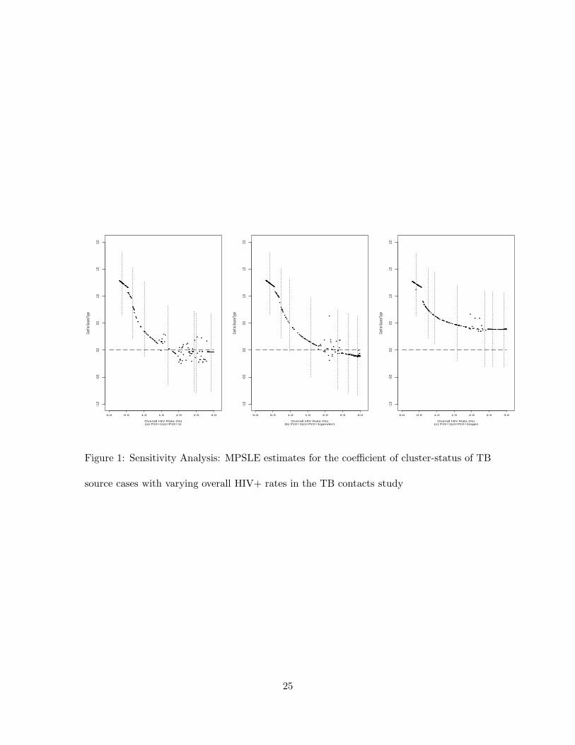
5.3 Additional sensitivity analysis

It was of the primary interest in the TB contact study to evaluate the effect of source

case cluster-status on the TB development of the contacts. The analysis presented above

reveals that the effect significance depends on the assumed HIV infection rate of all study

subjects. We conducted a sensitivity analysis to further explore the association. We sam-

pled from the linearly transformed Beta-distribution, 2.7%Beta(a, b) + 0.3%, with various

combinations of the Beta parameters (a, b): (1, 30), (1, 6), (1, 3), (3, 3), (3, 1), (6, 1), (30, 1).

All the samples ranged between 0.3% and 3% with the means associated with the above

pairs of (a, b) given by 0.39%, 0.68%, 0.97%, 1.7%, 2.3%, 2.6%, 2.9%, respectively, since the

Beta(a, b) distribution has mean a/(a+ b). With each of the realizations used as the “true”

value of P (X = 1), the pseudo-likelihood approach in Section 4 was implemented to analyze

the TB contact data under the three assumptions about P (X = 1 | Z) in Section 5.2. The

resulting outcomes, in agreement with the results in Table 2, were consistent with inferences

on significance of all the covariates except for the cluster-status of TB source cases. The

three plots in Figure 1 present the MPSLE estimates (points) along with the 2.5% and

97.5% percentiles (the vertical line segments) for the regression coefficient of the cluster-

status of TB source cases. The results associated with each of the aforementioned pairs

of (a, b) were based on 30 repetitions and presented at the sample mean of the generated

HIV rates. The plots show a trend of the dependence between estimated significance levels

17

of the cluster-status factor and the assumed overall HIV infection rates in the analysis. In

contrast to Figure 1 (a) and (b), Figure 1 (c) presents rather stable significance levels of

the cluster-status factor with high HIV infection rates stratified according to the age at

contact.

(Figure 1 is here.)

6 Discussion

When the missing covariate is missing at random (MAR), the approach in Section 3 reduces

to the approach in Herring and Ibrahim (2001), which uses the EM algorithm and estimates

the estimating function with the full covariate data. Specifically, in the E-step, Herring

and Ibrahim use the approximation E[S1(θ)/S0(θ)

]≈ ES1(θ)/ES0(θ), which leads to our

estimating equations (9) and (10).

A variation of Algorithm 1 is to substitute Step 1B with the following:

Step 1B∗: Evaluate xi in (11), and approximate eαxi and xieαxi by exiα and xiexiα,

respectively.

This variation of Algorithm 1 can be viewed as applying iteratively the conventional

partial likelihood approach under the Cox model with the missing xi imputed using the

current estimates of α, β and H0(·). It can be implemented in each iteration using the built-

in functions in Splus or R for the Cox regression with fully observed covariates. Further

investigation is required to study the asymptotic properties of the resulting estimators.

Practical applications of the procedure in Section 4 require that the dimension of Z(1)

and the number of its distinct values are both small enough, compared to the sample size

18

n, such that both n1(z(1)) and n(z(1)) are reasonably large for each z(1). To choose an

appropriate component vector of Z as Z(1) when X is an indicator, for example, we may

consider the logistic regression model,

P (X = 1 | R = 0, Z = z) = exp(η′

z(∗))/(1 + exp(η′

z(∗)))

with z(∗) composited of 1 and a component vector of z. Extending Algorithm 1, we can

then maximize the likelihood function (4), which now involves the parameter η, by solving

the estimating equations (5) together with ∂ logL(α, β, h0(·);G0)/∂η = 0 to attain the MLE

of α, β, h0(·) and η. The AIC and BIC variable selection procedures can be then applied

based on (4). However, the implementation could be computationally intensive, especially

when the dimension of Z is large. An alternative approach is to extend to situations with

missing covariates the method of Li, Dicker and Zhao (2010), who consider a new class of

Dantzig selectors for linear regression models with censored responses.

This paper assumes that all of the individuals in the study are independent. However,

in fact, the subjects in this example were clustered according to their TB source cases: TB

contacts who had the same TB source case were likely correlated and grouped together.

The current proposed approaches can be extended in principle to handle clustered study

subjects, if a correlation structure is assumed. It is usually challenging to specify a plausible

as well as feasible model to describe the correlation in practice.

The proposed approach requires the assumptions A1 and A2 in Section 2. There are

practical situations where either of the two assumptions is violated. In such situations, the

assumptions are probably plausible after having additional factors included in the covariate

list. If the new covariates are observable, the proposed approach is then applicable with the

19

new covariate list; otherwise, we may extend the proposed approach by applying a method

for handling latent covariates in the literature.

As suggested by a referee, it would be worthwhile exploring how the resulting inference in

Section 4 depends on the assumption of G0(· | Z) = G0(· | Z(1)), particularly when the true

model is G0(· | Z) = G0(· | Z(2)) with Z(2) a component vector of Z and containing Z(1) as

a component vector. Another further investigation is to develop Bayesian methodology for

handling the covariates missing not at random (MNAR), which may naturally incorporate

available prior information on the parameters.

Acknowledgments

The research was partially supported by grants from the Natural Sciences and Engineer-

ing Research Council of Canada (NSERC). We are very grateful to the editor, the associate

editor and the two referees for their helpful comments and suggestions, which have greatly

improved the paper. We thank Chunfang Lin for a preliminary numerical study and Jerry

Lawless for a helpful discussion.

References

Andersen, P.K., Borgan, O., Gill, R.D. and Keiding, N. (1992). Statistical Models Basedon Counting Processes, Springer, New York.

Bang, H. and Robins, J.M. (2005). “Doubly robust estimation in missing data and causalinference models,” Biometrics 61, 962-973.

Breslow, N.E. (1972). “Discussion of the paper by D. R. Cox,” J. R. Statist. Soc. B 34,216-217.

Canadian Tuberculosis Standards 6th Edition. Edited by Long, R. Canadian Lung Asso-ciation, Canadian Thoracic Society and Tuberculosis Prevention and Control Centrefor Infectious Disease Prevention and Control, Health Canada; 2007.

20

Chen, M.H., Ibrahim, J.G. and Shao, Q.M. (2009). “Maximum likelihood inference forthe Cox regression model with applications to missing covariates,” J. Multiv. Analys.100, 2018-2030.

Chen, H.Y. and Little, R.J.A. (1999). “Proportional Hazards Regression with MissingCovariates,” J. Amer. Statist. Assoc. 94, 896-908.

Cook, V.J., Hernandex-Garduno, E., Hu, X.J., Elwood, R.K. and FitzGerald, J.M. (2005).“The influence of cluster-status of source cases on contact evaluation and the develop-ment of secondary active tuberculosis,” Proceedings of the American Thoracic Society(PATS) 2005; 2 Abstract Issue.

Cox, D.R. (1972). “Regression models and life tables (with Discussion),” J. R. Statist Soc.B 34, 187-220.

Dempster, A.P., Laird, N.M. and Rubin, D.B. (1977). “Maximum likelihood from incom-plete data via the EM algorithm,” J. Roy. Statist. Soc. B 39, 1-22.

Efron, B. and Tibshirani, R.J. (1993). An Introduction to the Bootstrap, Monographs onStatistics and Applied Probability 57, CHAPMAN & HALL/CRC.

Herring, A.H. and Ibrahim, J.G. (2001). “Likelihood-based methods for missing covariatesin the Cox proportional hazards model,” J. Amer. Statist. Assoc. 96, 292-302.

HIV/AIDS Epi Updates November 2007, Centre for Infectious Disease Prevention andControl, Public Health Agency of Canada.

Hu, X.J. and Lawless, J.F. (1996). “Estimation from truncated lifetime data with supple-mentary information on covariates and censoring times,” Biometrika 83, 747-61.

Hu, X.J. and Lawless, J.F. (1997). “Pseudolikelihood estimation in a class of problemswith response-related missing covariates,” Can. J. Statist. 25, 125-42.

Li, Y., Dicker, L. and Zhao, S. (2010). “A new class of Dantzig selectors for censored linearregression models,” Harvard University Biostatistics Working Paper Series (March 2,2010).

Lin, D.Y. and Ying, Z. (1993). “Cox regression with incomplete covariate measurements,”J. Amer. Statist. Assoc. 88, 1341-9.

Little, R.J.A. and Rubin, D.B. (2002). Statistical Analysis with Missing Data, Wiley Seriesin Probability and Statistics, Wiley.

Nan, B., Kalbfleisch, J.D. and Yu, M. (2009). “Asymptotic theory for the semiparametricaccelerated failure time model with missing data,” Ann. Statist. 37, 2351-2376.

Paik, M.C. and Tsai, W.Y. (1997). “On using the Cox proportional hazards model withmissing covariates,” Biometrika 84, 579-593.

Qi, L., Wang, C.Y., and Prentice, R.L. (2005). “Weighted estimators for proportionalhazards regression with missing covariates,” J. Amer. Statist. Assoc. 100, 1250-63.

21

Reichler, M.R., Bur, S., Reves, R., Mangura, B., Thompson, V., Ford, J. and Castro, K.G.(2003). “Results of testing for human immunodeficiency virus infection among recentcontacts of infectious tuberculosis cases in the United States,” Int. J. Tuberc. LungDis. 7(12): 5471-5478.

Robins, J.M., Rotnitzky, A. and Zhao, L.P. (1994). “Estimation of regression coefficientswhen some regressors are not always observed,” J. Amer. Statist. Assoc. 89, 846-66.

Scharfstein, D.O., Rotnitzky, A. and Robins, J.M. (1999). “Adjusting for nonignorabledrop-out using semiparametric nonresponse models,” J. Amer. Statist. Assoc. 94,1096-1120.

Suzuki, K. (1985). “Estimation method of lifetime based on the record of failures duringthe warranty period,” J. Amer. Statist. Assoc. 80, 68-72.

Tsiatis, A.A. (2006). Semiparametric Theory and Missing Data, Springer Series in Statis-tics, SPRINGER.

Zeng, D. and Cai, J. (2005). “Asymptotic results for maximum likelihood estimators injoint analysis of repeated measurements and survival time,” Ann. Statist. 33, 2132-2163.

Zhou, H. and Pepe, M.S. (1995). “Auxiliary covariate data in failure time regression,”Biometrika 82, 139-149.

22

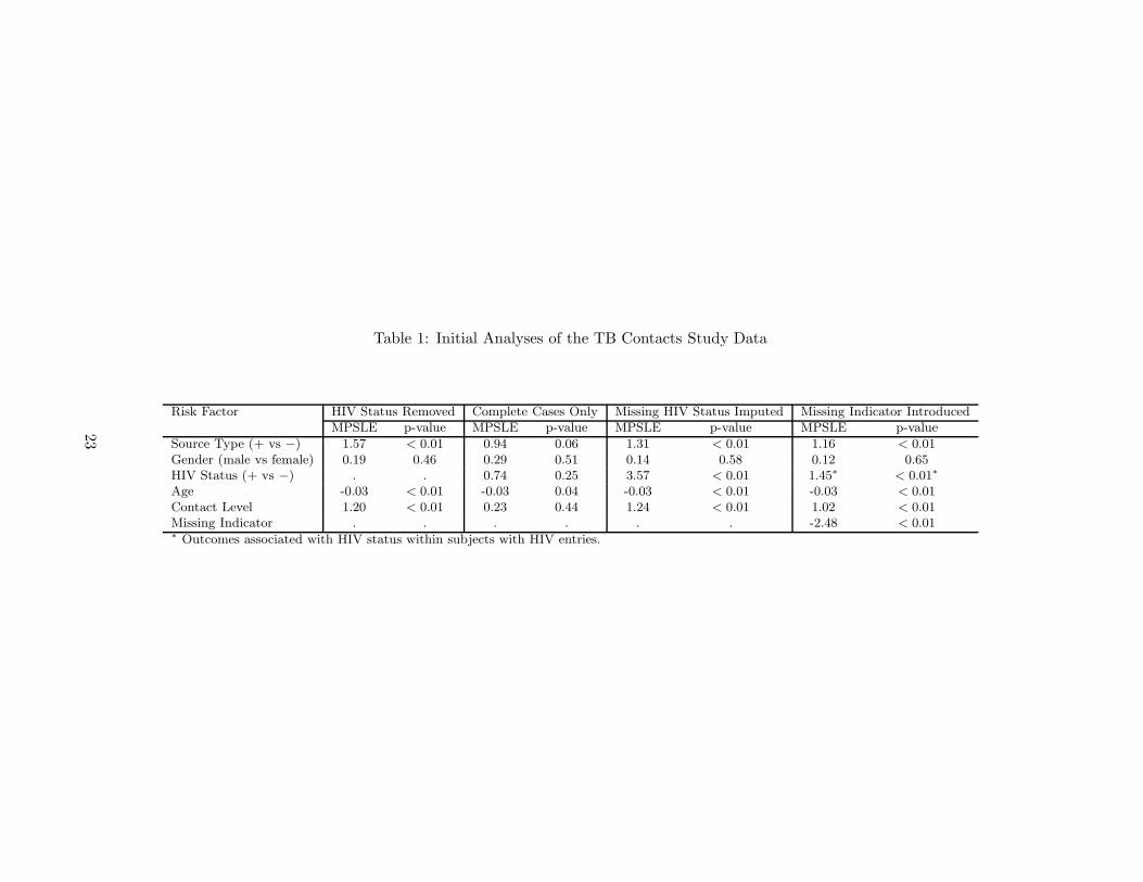
Table 1: Initial Analyses of the TB Contacts Study Data

Risk Factor HIV Status Removed Complete Cases Only Missing HIV Status Imputed Missing Indicator IntroducedMPSLE p-value MPSLE p-value MPSLE p-value MPSLE p-value

Source Type (+ vs −) 1.57 < 0.01 0.94 0.06 1.31 < 0.01 1.16 < 0.01Gender (male vs female) 0.19 0.46 0.29 0.51 0.14 0.58 0.12 0.65HIV Status (+ vs −) . . 0.74 0.25 3.57 < 0.01 1.45∗ < 0.01∗

Age -0.03 < 0.01 -0.03 0.04 -0.03 < 0.01 -0.03 < 0.01Contact Level 1.20 < 0.01 0.23 0.44 1.24 < 0.01 1.02 < 0.01Missing Indicator . . . . . . -2.48 < 0.01∗ Outcomes associated with HIV status within subjects with HIV entries.

23

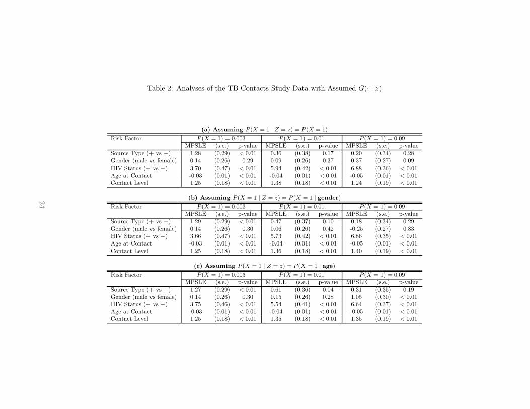
Table 2: Analyses of the TB Contacts Study Data with Assumed G(· | z)

(a) Assuming P (X = 1 | Z = z) = P (X = 1)

Risk Factor P (X = 1) = 0.003 P (X = 1) = 0.01 P (X = 1) = 0.09MPSLE (s.e.) p-value MPSLE (s.e.) p-value MPSLE (s.e.) p-value

Source Type (+ vs −) 1.28 (0.29) < 0.01 0.36 (0.38) 0.17 0.20 (0.34) 0.28Gender (male vs female) 0.14 (0.26) 0.29 0.09 (0.26) 0.37 0.37 (0.27) 0.09HIV Status (+ vs −) 3.70 (0.47) < 0.01 5.94 (0.42) < 0.01 6.88 (0.36) < 0.01Age at Contact -0.03 (0.01) < 0.01 -0.04 (0.01) < 0.01 -0.05 (0.01) < 0.01Contact Level 1.25 (0.18) < 0.01 1.38 (0.18) < 0.01 1.24 (0.19) < 0.01

(b) Assuming P (X = 1 | Z = z) = P (X = 1 | gender)

Risk Factor P (X = 1) = 0.003 P (X = 1) = 0.01 P (X = 1) = 0.09MPSLE (s.e.) p-value MPSLE (s.e.) p-value MPSLE (s.e.) p-value

Source Type (+ vs −) 1.29 (0.29) < 0.01 0.47 (0.37) 0.10 0.18 (0.34) 0.29Gender (male vs female) 0.14 (0.26) 0.30 0.06 (0.26) 0.42 -0.25 (0.27) 0.83HIV Status (+ vs −) 3.66 (0.47) < 0.01 5.73 (0.42) < 0.01 6.86 (0.35) < 0.01Age at Contact -0.03 (0.01) < 0.01 -0.04 (0.01) < 0.01 -0.05 (0.01) < 0.01Contact Level 1.25 (0.18) < 0.01 1.36 (0.18) < 0.01 1.40 (0.19) < 0.01

(c) Assuming P (X = 1 | Z = z) = P (X = 1 | age)

Risk Factor P (X = 1) = 0.003 P (X = 1) = 0.01 P (X = 1) = 0.09MPSLE (s.e.) p-value MPSLE (s.e.) p-value MPSLE (s.e.) p-value

Source Type (+ vs −) 1.27 (0.29) < 0.01 0.61 (0.36) 0.04 0.31 (0.35) 0.19Gender (male vs female) 0.14 (0.26) 0.30 0.15 (0.26) 0.28 1.05 (0.30) < 0.01HIV Status (+ vs −) 3.75 (0.46) < 0.01 5.54 (0.41) < 0.01 6.64 (0.37) < 0.01Age at Contact -0.03 (0.01) < 0.01 -0.04 (0.01) < 0.01 -0.05 (0.01) < 0.01Contact Level 1.25 (0.18) < 0.01 1.35 (0.18) < 0.01 1.35 (0.19) < 0.01

24

(a) P(X=1|z)=P(X=1)Overall HIV Rate (%)

Coef

to So

urceT

ype

0.0 0.5 1.0 1.5 2.0 2.5 3.0

−1.0

−0.5

0.00.5

1.01.5

2.0

•

••••••

••

••

•••

•

•

•

•••••

••••

•

•

•

•

•

•

•

•

•

•

•

•

••••

•

•

•

•

•

•

•

•

•

••

•

•

•

•

•

•

•

•

•

•

•

•

•

••

•

•

•

•

•

•

•

•

•

•

•

•

•••

•

•

•

•

•

•

•

•

•

•

•

•

•

•

•

•

•

•

•

•

• •

•

•

•

•

•

•

•

•

••

• •

•

•

•

•

•

•

•

•

•

••• •

•

•

•

•

• •

•

•

•

•

••

•

•

•

••

•

•

• •

• •

•

•

•

•

•

••

•

•

•• ••

•

•

•

•

•

• •

•

•

•

•

•

•

• ••• •••••• ••• ••

•

•

•

••••• ••• •••

•

••••••

••

••

•••

•

•

•

•••••

••••

•

•

•

•

•

•

•

•

•

•

•

•

••••

•

•

•

•

•

•

•

•

•

••

•

•

•

•

•

•

•

•

•

•

•

•

•

••

•

•

•

•

•

•

•

•

•

•

•

•

•••

•

•

•

•

•

•

•

•

•

•

•

•

•

•

•

•

•

•

•

•

• •

•

•

•

•

•

•

•

•

••

• •

•

•

•

•

•

•

•

•

•

••• •

•

•

•

•

• •

•

•

•

•

••

•

•

•

••

•

•

• •

• •

•

•

•

•

•

••

•

•

•• ••

•

•

•

•

•

• •

•

•

•

•

•

•

• ••• •••••• ••• ••

•

•

•

••••• ••• •••

(b) P(X=1|z)=P(X=1|gender)Overall HIV Rate (%)

Coef

to So

urceT

ype

0.0 0.5 1.0 1.5 2.0 2.5 3.0

−1.0

−0.5

0.00.5

1.01.5

2.0

••••••••

•

••••

••

•

•••••

•

••

•••

•

••

•

••

•

•

•

•

•

•

••

••

•

•

•

•

••

•

•

•

•

•

•••

••

••

•

••

•

•

•

•

•

•

•

•

•

•

•

•

•

•

•

•

•

•

•

•

•

••

•

•

•

•

•

•

•

•

•

•

••

•

•

•

•

•

•

••

•

•

••

•

•

• •

•

•

•

•

•

••

•

•

••

••

• •• ••

•

•

•

•

•

•

••

•

•••••

•

•

•

• ••

•

••

•

•

•

•

•

• •• ••

•

•

•

••• •

••

••

••

• •• •• •

•• • •••••• •• ••••••••••••• •

••••••••

•

••••

••

•

•••••

•

••

•••

•

••

•

••

•

•

•

•

•

•

••

••

•

•

•

•

••

•

•

•

•

•

•••

••

••

•

••

•

•

•

•

•

•

•

•

•

•

•

•

•

•

•

•

•

•

•

•

•

••

•

•

•

•

•

•

•

•

•

•

••

•

•

•

•

•

•

••

•

•

••

•

•

• •

•

•

•

•

•

••

•

•

••

••

• •• ••

•

•

•

•

•

•

••

•

•••••

•

•

•

• ••

•

••

•

•

•

•

•

• •• ••

•

•

•

••• •

••

••

••

• •• •• •

•• • •••••• •• ••••••••••••• •

(c) P(X=1|z)=P(X=1|age)Overall HIV Rate (%)

Coef

to So

urceT

ype

0.0 0.5 1.0 1.5 2.0 2.5 3.0

−1.0

−0.5

0.00.5

1.01.5

2.0

•••••

• •••

• •••

•••••

•

•••

••

••

•••••

•

•••

•

•

•

•

•

•

••

•

•

•

•

•

•

•

•

•

•

••

•

•

•

•

••

•

•

•

•

•

•••

•

••

•

•

••

•

•

••

•

•

•

•

•

••

•

•

•

•••

•

•

••

•

•

• •

•

•

•

•

••

•

•••

•

•

•

•

•

••••

••••

••• •• •

•

•

• •• • •

•

•••••

• •••

• •• ••

••

•• ••

•

• ••• • ••• ••• •• •• •••

•

••••••• •• •• • • ••••••••••• • •••• •

•••••

• •••

• •••

•••••

•

•••

••

••

•••••

•

•••

•

•

•

•

•

•

••

•

•

•

•

•

•

•

•

•

•

••

•

•

•

•

••

•

•

•

•

•

•••

•

••

•

•

••

•

•

••

•

•

•

•

•

••

•

•

•

•••

•

•

••

•

•

• •

•

•

•

•

••

•

•••

•

•

•

•

•

••••

••••

••• •• •

•

•

• •• • •

•

•••••

• •••

• •• ••

••

•• ••

•

• ••• • ••• ••• •• •• •••

•

••••••• •• •• • • ••••••••••• • •••• •

Figure 1: Sensitivity Analysis: MPSLE estimates for the coefficient of cluster-status of TB

source cases with varying overall HIV+ rates in the TB contacts study

25