semiparametric mixed effects models with flexible …davidian/semitalk.pdf · semiparametric mixed...
TRANSCRIPT

Semiparametric Mixed Effects Models withFlexible Random Effects Distribution
Marie Davidian∗
North Carolina State University
www.stat.ncsu.edu/˜davidian
∗Joint work with A. Tsiatis, J. Chen, X. Song, and D. Zhang

Outline
1. Introduction and motivation
2. Semiparametric mixed models
3. The class H and the SNP representation
4. Implementation
5. Simulations
6. Examples, revisited
7. Discussion

1. Introduction and motivationLongitudinal studies: Clinical trials, epidemiological investigations
• Repeated measures on some variable on each subjectintermittently over time
• Survival endpoint (e.g., death, time to disease progression)
Objectives: Inference on
• Within-subject patterns of change of repeated measurementvariable, association with covariates
• Relationship between repeated measurement variable andsurvival, association with covariates

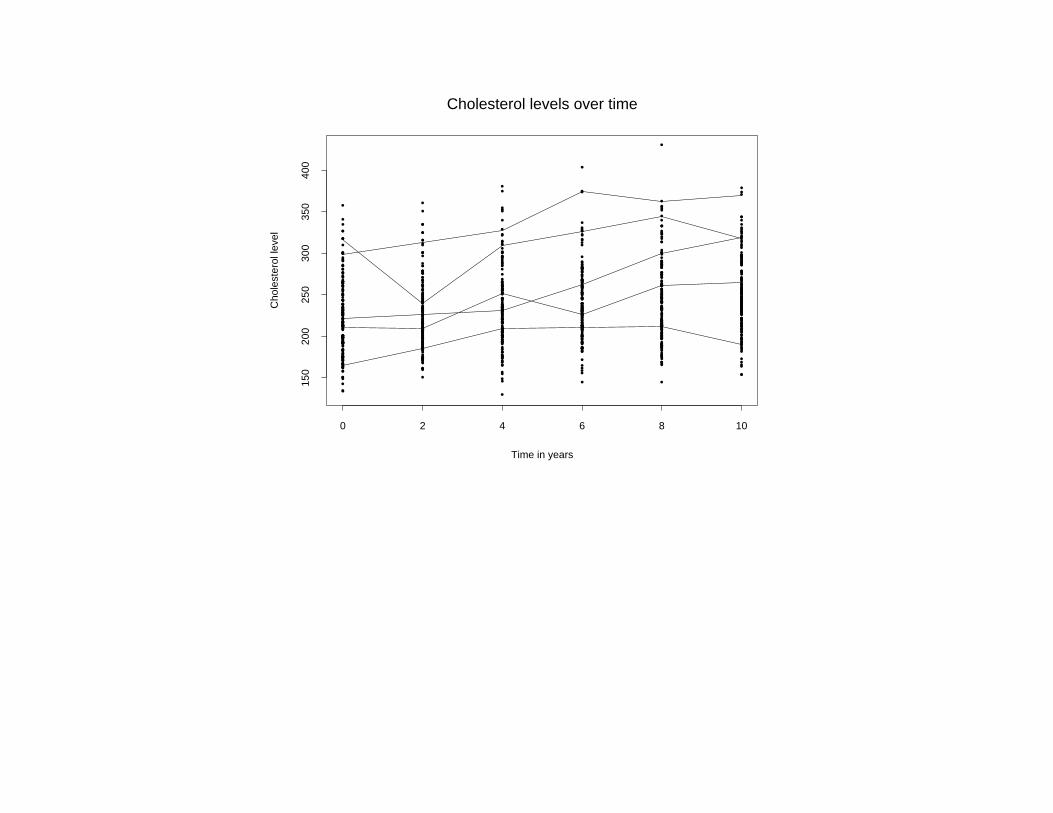
Example 1: Framingham study
• Cholesterol measurements every 2 years for 2634 participantsover 10-year period
• Objectives: Change in cholesterol over time and associationwith age at baseline, gender
• Consider a subset of 200 subjects for illustrative purposes
Individual profiles: Approximate straight line
•
• •
•• •
•
•
••
•
•
••
•• •
•
••
•
•
•• •
•
• • ••
•
•
•
•
•
••
•
•
•
•
•
• •• •
•
•• •
•
•
••
••
• • ••
• •
•
•• •
•
••
••
• •••
•
•
•
•
•• • •
•
•
••
••
•• •
••
• ••
•
•
•
•
••
•
•
•• •
•
•
•
•
• •• •
•
•
•
•
•• •
•
• •
•
• ••
•
••
•
•
• •
•
•
•
••
• •
•
•
•
•
••
• •
• •••
• •
•
•
••
•
•
••
•
•
•
••
• ••
•
••
•
•
•
•
••
•
•
• •
•
•
•• •
•
•
• •
••
•
•
•
•
•
•
••
•
• • ••
• •
•
••
• ••
•
••
• •
••
• ••
•
••
•
• • • •
••
••
••
•
••
•
•
•
•
• •• •
•
• •• •
•
•
• •• • •
••
••
•
•
•
• •
•
• •
•
••
••
•
••
••
•
•
• •
• • ••
•
•
••
•
••
•
•
•
•
•
••
••
• •
•
•
•
•
•
•
•
••
•• •
•
••
•
••
•
•
••
••
•
• •
• •
••• • •
••
•
••
• •
•
•• • •
•
•
••
•
•
•
•
•
•
• • •
•
•• •
•
•
•
••
••
•
•
•
••
••
• •
•
•
••
•
•
•
•
••
••
•
•
•
• •
•
• • •
••
• ••
• • ••
• • •
•
•
•
•
•• •
•
•
•
••
•
•
•
••
••
•
• •
•• •
•
•
•
• • •
•
•
•
•
•
•
••
•••
•
•• •
•
•
•
••
•
••
• •
•
• •
• • • •
• •
• • ••
••
•• • • •
•
• •• • •
•
••
•
••
•
•
•
••
••
•
•
••
•
••
•• •
••
•
••
•
•
••
•
• ••
••
•
••
••
•
•
•• • •
•• •
•
•
•
•
• •
•
•
• •
•
• ••
•
•
•
•
•• •
• •
•
•
•
•
•
•
•
•
••
•
•
•
••
• ••
••
•• •
••
• •
•
•
•
••
•
•
••
•
• ••
••
•
•
••
•
•
•
••
••
•
•
•
•
•
• •
••
•
•
• • •
• •
• ••
•
• •
•
••
•
•
••
• ••
•
••
• • • • ••
•
••
•
• •
•
••
••
• ••
•
•
•
•• •
•
•
•
•
••
• ••
•
••
••
•
•
•
•
•
•• •
••
•
•
•
•
•
••
•
••
••
••
•
••
•
• •
•
• •• •
•
• •
••
•
• •
••
•
•
•
••
•
•
•
•
••
•
•
••
• • •
••
••
••
•
••
•
•
•• •
•
•
•
••
• •
•
• •
•
• • ••
•
• •
•
•• ••
•
• •
••
•
•
•
•
•
••
•
•
•
••
•
••
•
••
•
•
••
••
••
•
•
••
•
•
••
•
•
• • •
•
•
•
•
••
•
•
••
• ••
•
•• •
•
•
•
• •
•
•
••
••
•
• •
•
••
•
•
•
• ••
•
••
•
•
•
•
•
•
•
•
•
•
•
•
•
••
• •
••
•
• •
•
•
•
•
••
•• •
••
•
•
•• •
•
• • •
•
•• •
• •
•••
••
••
••
••
•
•
• •
• • ••
•
•
••
•
•
• •
•
•
•
•
•
••
•
••
•
•
• •
•••
••
•
• •
• •
•
••
••
•
•
•
• •
•
••
•
•
••
•
•
•
•
•
• ••
•
••
• •
•
•
•
•
•
•
• •
•
••
•• •
•
•
Time in years
Cho
lest
erol
leve
l
0 2 4 6 8 10
150
200
250
300
350
400
Cholesterol levels over time
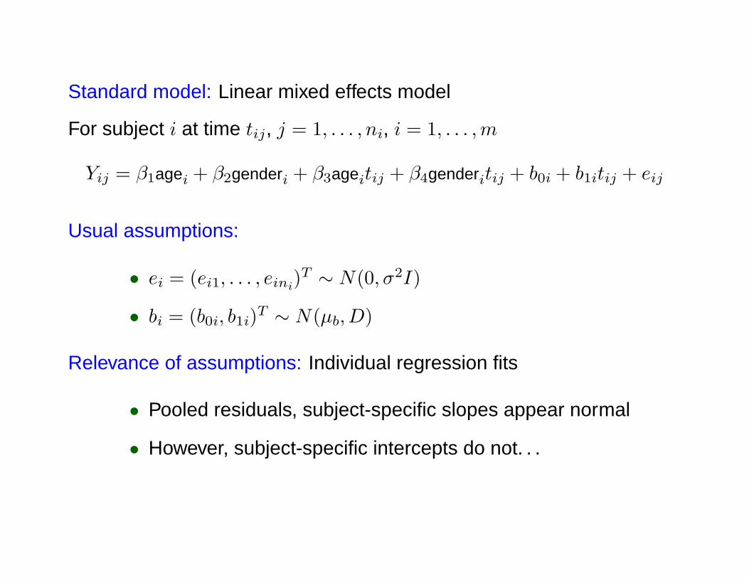
Standard model: Linear mixed effects model
For subject i at time tij, j = 1, . . . , ni, i = 1, . . . ,m
Yij = β1agei + β2genderi + β3ageitij + β4genderitij + b0i + b1itij + eij
Usual assumptions:
• ei = (ei1, . . . , eini)T ∼ N(0, σ2I)
• bi = (b0i, b1i)T ∼ N(µb, D)
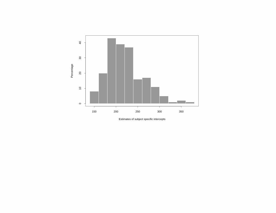
Relevance of assumptions: Individual regression fits
• Pooled residuals, subject-specific slopes appear normal
• However, subject-specific intercepts do not. . .
150 200 250 300 350
010
2030
40
Estimates of subject specific intercepts
Per
cent
age
Example 2: Six cities study
• Binary indicator of respiratory infection recored annually for537 Ohio children at ages 7–10
• Objectives: Within-subject change in respiratory status,association with baseline maternal smoking
Standard model: Generalized linear mixed effects model
For subject i at age aij, j = 1, . . . , ni, i = 1, . . . ,m
E(Yij|bi) =exp(β1smoke + β2aij + bi)
1 + exp(β1smoke + β2aij + bi), var(Yij|bi) = E(Yij|bi)1−E(Yij|bi)
Usual assumption: bi ∼ N(µb, σ2b)

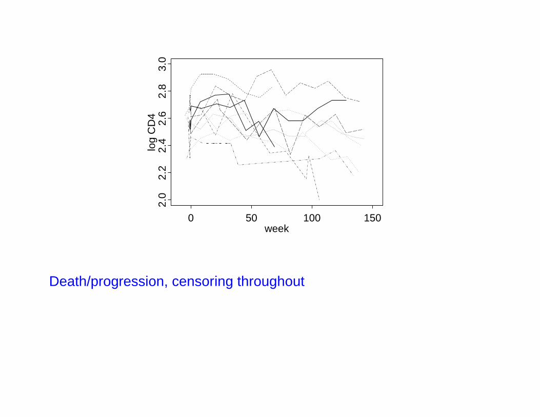
Example 3: ACTG 175
• Clinical trial with 2467 subjects to compare 4 antiretroviralregimens
• Main objective: Compare on basis of time to AIDS or death
• Also, CD4 counts approximately every 12 weeks
• Subsequent objective: Characterize within-subject patterns ofCD4 change – complicated by informative censoring
• Subsequent objective: Characterize relationship betweenfeatures of CD4 profiles and survival
week
log
CD
4
0 50 100 150
2.0
2.2
2.4
2.6
2.8
3.0
Death/progression, censoring throughout
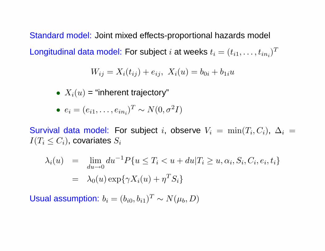
Standard model: Joint mixed effects-proportional hazards model
Longitudinal data model: For subject i at weeks ti = (ti1, . . . , tini)T
Wij = Xi(tij) + eij, Xi(u) = b0i + b1iu
• Xi(u) = “inherent trajectory”
• ei = (ei1, . . . , eini)T ∼ N(0, σ2I)
Survival data model: For subject i, observe Vi = min(Ti, Ci), ∆i =I(Ti ≤ Ci), covariates Si
λi(u) = limdu→0
du−1Pu ≤ Ti < u+ du|Ti ≥ u, αi, Si, Ci, ei, ti
= λ0(u) expγXi(u) + ηTSi
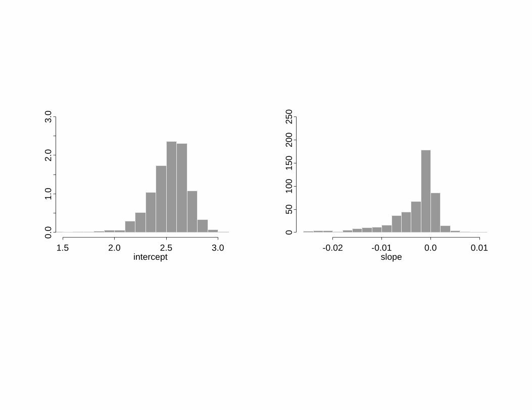
Usual assumption: bi = (bi0, bi1)T ∼ N(µb, D)
1.5 2.0 2.5 3.0
0.0
1.0
2.0
3.0
intercept-0.02 -0.01 0.0 0.01
050
100
150
200
250
slope
2. Semiparametric mixed models
Theme: The foregoing examples suggest that
• A simple parametric model may be adequate to describesubject-specific profiles in terms of random effects bi
• However, the relevance of the usual normality assumption onrandom effects is questionable
Concern: Sensitivity of inferences to departures from normality
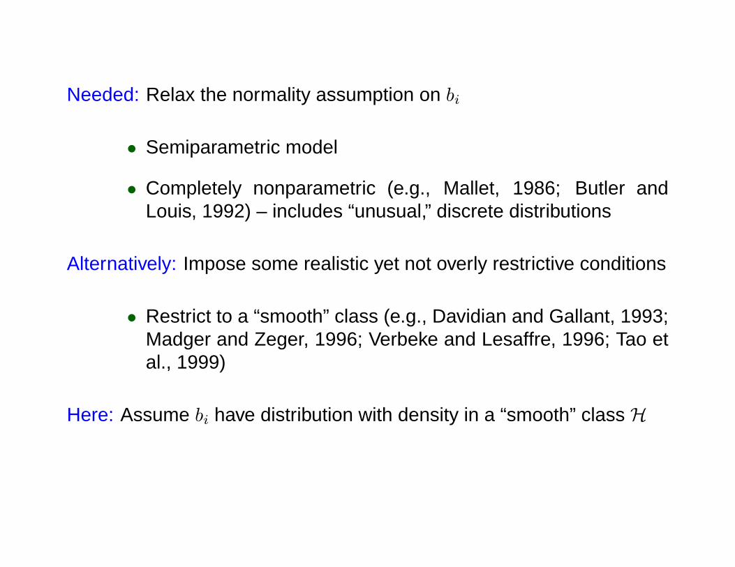
Needed: Relax the normality assumption on bi
• Semiparametric model
• Completely nonparametric (e.g., Mallet, 1986; Butler andLouis, 1992) – includes “unusual,” discrete distributions
Alternatively: Impose some realistic yet not overly restrictive conditions
• Restrict to a “smooth” class (e.g., Davidian and Gallant, 1993;Madger and Zeger, 1996; Verbeke and Lesaffre, 1996; Tao etal., 1999)
Here: Assume bi have distribution with density in a “smooth” class H
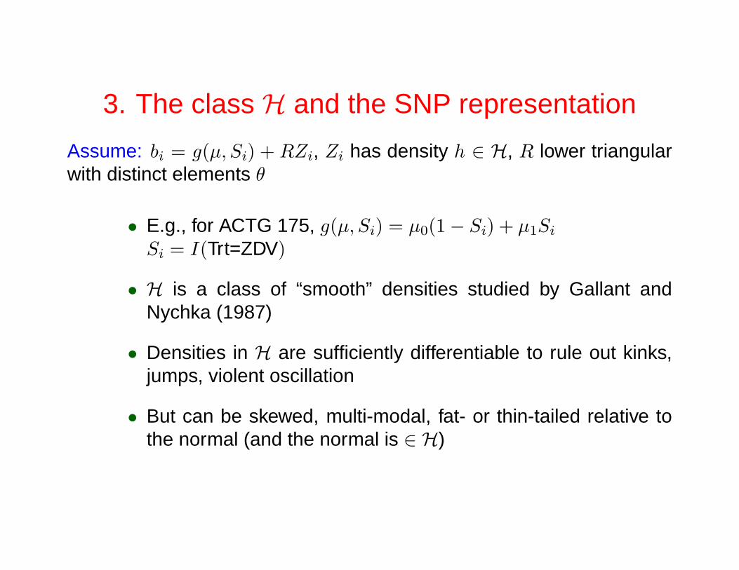
3. The class H and the SNP representation
Assume: bi = g(µ, Si) + RZi, Zi has density h ∈ H, R lower triangularwith distinct elements θ
• E.g., for ACTG 175, g(µ, Si) = µ0(1− Si) + µ1SiSi = I(Trt=ZDV)
• H is a class of “smooth” densities studied by Gallant andNychka (1987)
• Densities in H are sufficiently differentiable to rule out kinks,jumps, violent oscillation
• But can be skewed, multi-modal, fat- or thin-tailed relative tothe normal (and the normal is ∈ H)
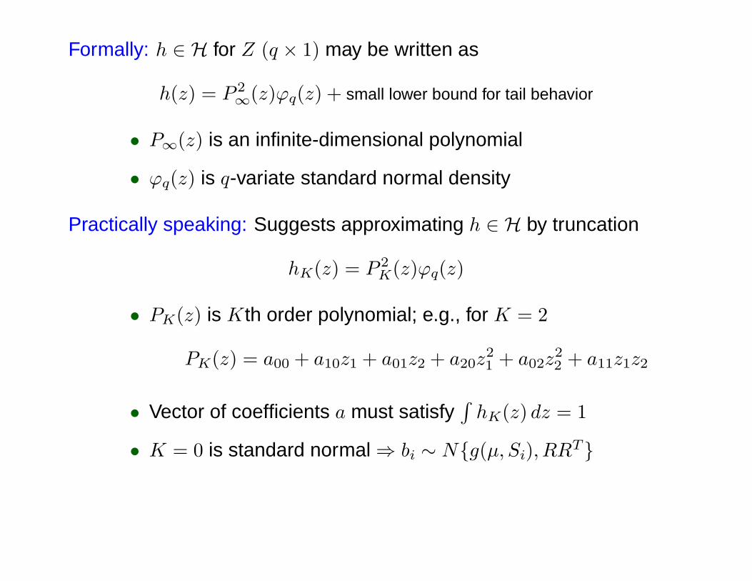
Formally: h ∈ H for Z (q × 1) may be written as
h(z) = P 2∞(z)ϕq(z) + small lower bound for tail behavior
• P∞(z) is an infinite-dimensional polynomial
• ϕq(z) is q-variate standard normal density
Practically speaking: Suggests approximating h ∈ H by truncation
hK(z) = P 2K(z)ϕq(z)
• PK(z) is Kth order polynomial; e.g., for K = 2
PK(z) = a00 + a10z1 + a01z2 + a20z21 + a02z
22 + a11z1z2
• Vector of coefficients a must satisfy∫hK(z) dz = 1
• K = 0 is standard normal⇒ bi ∼ Ng(µ, Si), RRT
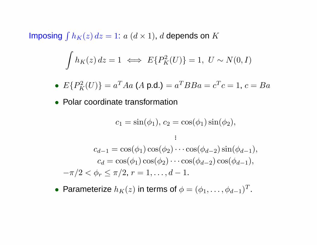
Imposing∫hK(z) dz = 1: a (d× 1), d depends on K∫hK(z) dz = 1 ⇐⇒ EP 2
K(U) = 1, U ∼ N(0, I)
• EP 2K(U) = aTAa (A p.d.) = aTBBa = cT c = 1, c = Ba
• Polar coordinate transformation
c1 = sin(φ1), c2 = cos(φ1) sin(φ2),...
cd−1 = cos(φ1) cos(φ2) · · · cos(φd−2) sin(φd−1),cd = cos(φ1) cos(φ2) · · · cos(φd−2) cos(φd−1),
−π/2 < φr ≤ π/2, r = 1, . . . , d− 1.
• Parameterize hK(z) in terms of φ = (φ1, . . . , φd−1)T .
Result: For fixedK, may represent density of bi in terms of (µT , θT , φT )T
• Likelihood for Ω = (µT , θT , φT )T plus any other modelparameters (e.g., β, γ, η) is usual, finite-dimensional problem
• In principle, can use standard optimization methods toestimate Ω (coming up. . . )
Lingo: “Seminonparametric”
Choosing tuning parameter K: K controls degree of flexibility anddeparture from normality (like a “bandwidth”)
Adaptive choice of K based on information criteria:
• If `K(Ω) is maximized loglikelihood for fixed K, N = totalnumber of observations, Ω (p× 1), minimize
−`K(Ω) + pC(N)/N
• AIC, C(N) = 1; BIC, C(N) = logN/2;Hannan-Quinn (HQ), C(N) = log logN
• AIC prefers “larger” models, BIC “smaller,” HQ intermediate
• Confidence intervals fixing K at choice achieve nominalcoverage (Eastwood and Gallant, 1991)
4. Implementation
Linear mixed effects model: For normal ei, Ω = (µT , θT , φT , βT , σ)T , canwrite loglikelihood `K(Ω; Y ) in a closed form
• Maximize in Ω using standard optimization routines, e.g.,SAS nlpqn
• Starting values chosen by grid search or penalizedloglikelihood
• SEs, confidence intervals – usual inverse of observedinformation for chosen K
• Zhang and Davidian (2001, Biometrics)
Generalized linear mixed effects model: Other models (e.g., binomial,Poisson), Ω = (µT , θT , φT , βT )T , cannot write `K(Ω; Y ) in a closed form
• Gallant and Tauchen (1992) provide efficient rejectionsampling algorithm from estimated hK(z) (acceptance rate >50%)
• Facilitates use of MCEM algorithm (e.g., McCulloch, 1997;Booth and Hobert, 1999)
• SEs, confidence intervals – MC approx observed informationfor chosen K
• Chen, Zhang, and Davidian (2002, Biostatistics)
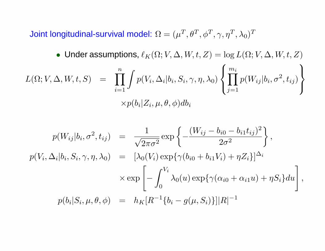
Joint longitudinal-survival model: Ω = (µT , θT , φT , γ, ηT , λ0)T
• Under assumptions, `K(Ω;V,∆,W, t, Z) = logL(Ω;V,∆,W, t, Z)
L(Ω;V,∆,W, t, S) =n∏i=1
∫p(Vi,∆i|bi, Si, γ, η, λ0)
mi∏j=1
p(Wij|bi, σ2, tij)
×p(bi|Zi, µ, θ, φ)dbi
p(Wij|bi, σ2, tij) =1√
2πσ2exp
−(Wij − bi0 − bi1tij)2
2σ2
,
p(Vi,∆i|bi, Si, γ, η, λ0) = [λ0(Vi) expγ(bi0 + bi1Vi) + ηZi]∆i
× exp
[−∫ Vi
0
λ0(u) expγ(αi0 + αi1u) + ηSidu
],
p(bi|Si, µ, θ, φ) = hK[R−1bi − g(µ, Si)]|R|−1
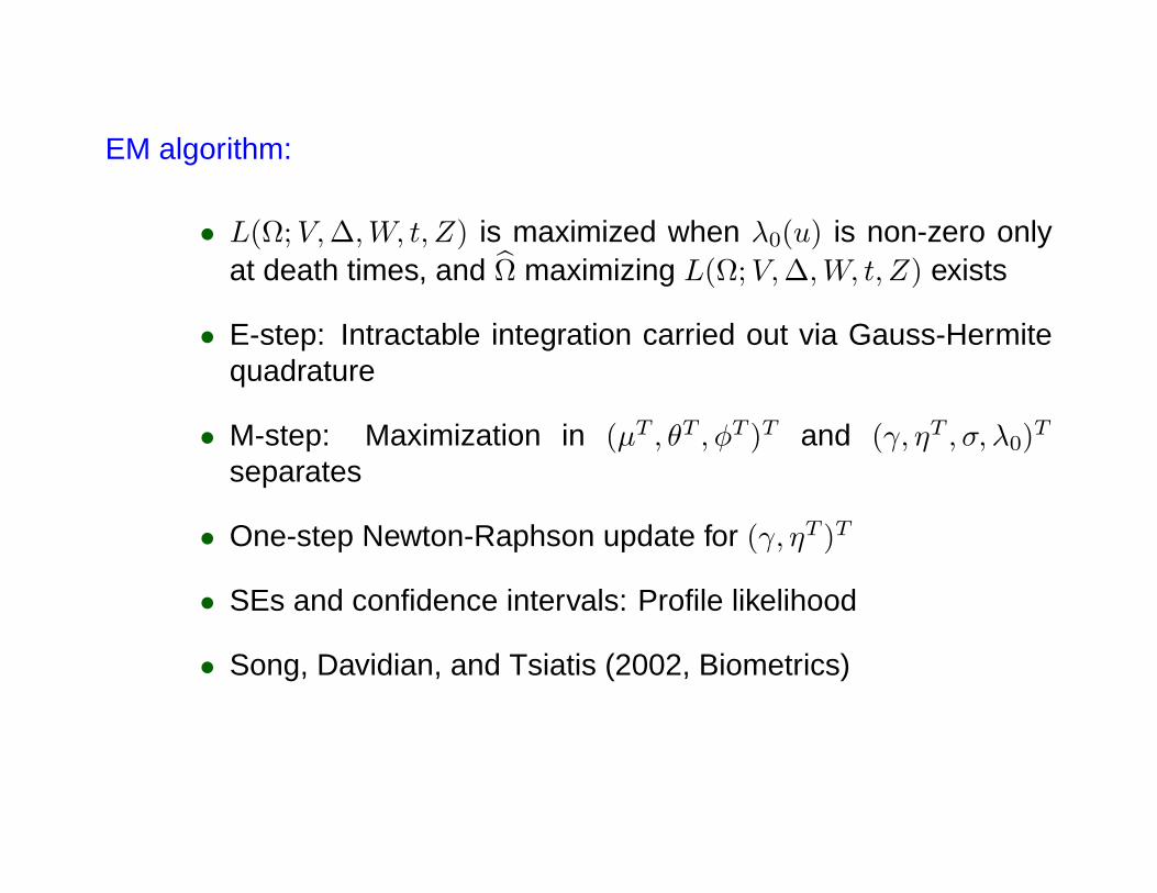
EM algorithm:
• L(Ω;V,∆,W, t, Z) is maximized when λ0(u) is non-zero onlyat death times, and Ω maximizing L(Ω;V,∆,W, t, Z) exists
• E-step: Intractable integration carried out via Gauss-Hermitequadrature
• M-step: Maximization in (µT , θT , φT )T and (γ, ηT , σ, λ0)T
separates
• One-step Newton-Raphson update for (γ, ηT )T
• SEs and confidence intervals: Profile likelihood
• Song, Davidian, and Tsiatis (2002, Biometrics)
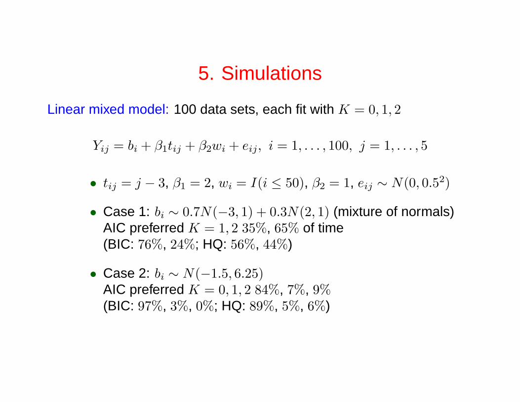
5. Simulations
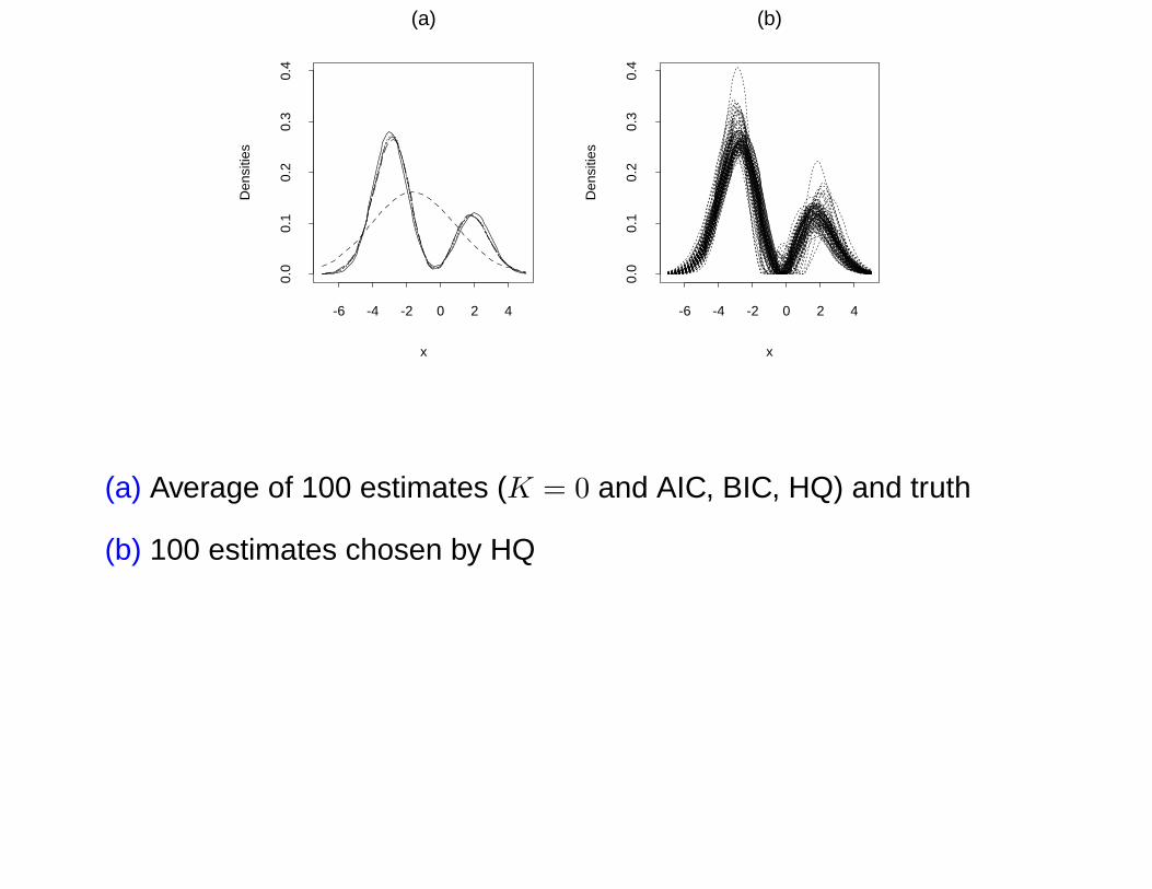
Linear mixed model: 100 data sets, each fit with K = 0, 1, 2
Yij = bi + β1tij + β2wi + eij, i = 1, . . . , 100, j = 1, . . . , 5
• tij = j − 3, β1 = 2, wi = I(i ≤ 50), β2 = 1, eij ∼ N(0, 0.52)
• Case 1: bi ∼ 0.7N(−3, 1) + 0.3N(2, 1) (mixture of normals)AIC preferred K = 1, 2 35%, 65% of time(BIC: 76%, 24%; HQ: 56%, 44%)
• Case 2: bi ∼ N(−1.5, 6.25)AIC preferred K = 0, 1, 2 84%, 7%, 9%(BIC: 97%, 3%, 0%; HQ: 89%, 5%, 6%)
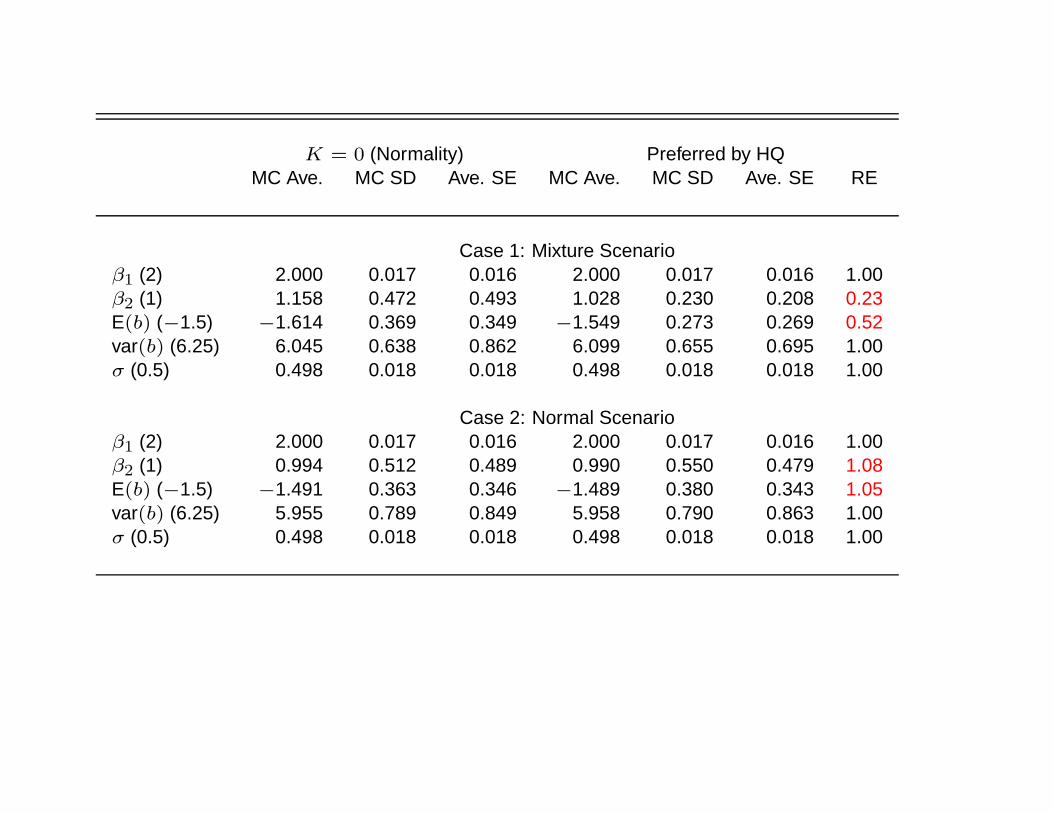
K = 0 (Normality) Preferred by HQMC Ave. MC SD Ave. SE MC Ave. MC SD Ave. SE RE
Case 1: Mixture Scenarioβ1 (2) 2.000 0.017 0.016 2.000 0.017 0.016 1.00β2 (1) 1.158 0.472 0.493 1.028 0.230 0.208 0.23E(b) (−1.5) −1.614 0.369 0.349 −1.549 0.273 0.269 0.52var(b) (6.25) 6.045 0.638 0.862 6.099 0.655 0.695 1.00σ (0.5) 0.498 0.018 0.018 0.498 0.018 0.018 1.00
Case 2: Normal Scenarioβ1 (2) 2.000 0.017 0.016 2.000 0.017 0.016 1.00β2 (1) 0.994 0.512 0.489 0.990 0.550 0.479 1.08E(b) (−1.5) −1.491 0.363 0.346 −1.489 0.380 0.343 1.05var(b) (6.25) 5.955 0.789 0.849 5.958 0.790 0.863 1.00σ (0.5) 0.498 0.018 0.018 0.498 0.018 0.018 1.00
x
Den
sitie
s
-6 -4 -2 0 2 4
0.0
0.1
0.2
0.3
0.4
(a)
x
Den
sitie
s
-6 -4 -2 0 2 4
0.0
0.1
0.2
0.3
0.4
(b)
(a) Average of 100 estimates (K = 0 and AIC, BIC, HQ) and truth
(b) 100 estimates chosen by HQ
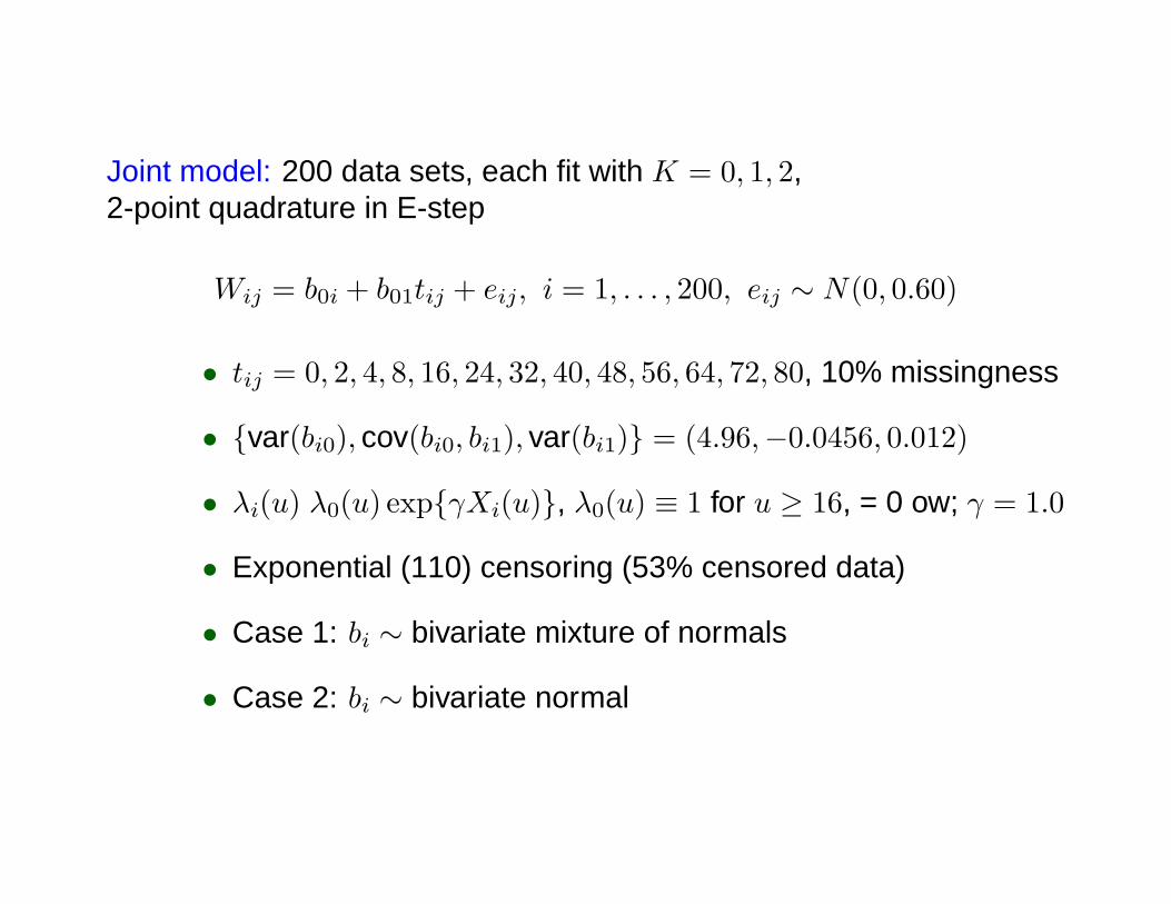
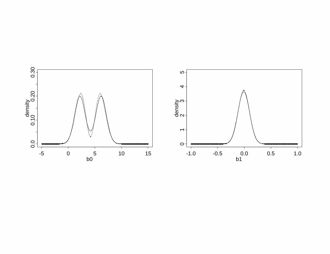
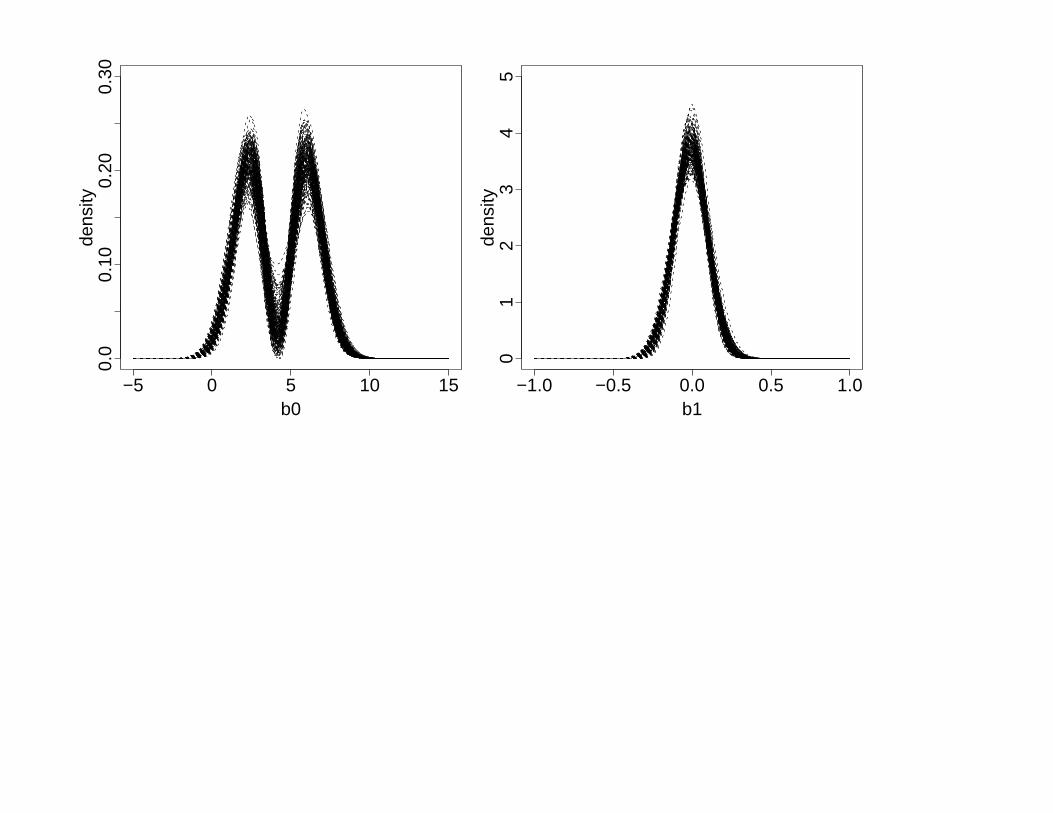
Joint model: 200 data sets, each fit with K = 0, 1, 2,2-point quadrature in E-step
Wij = b0i + b01tij + eij, i = 1, . . . , 200, eij ∼ N(0, 0.60)
• tij = 0, 2, 4, 8, 16, 24, 32, 40, 48, 56, 64, 72, 80, 10% missingness
• var(bi0), cov(bi0, bi1), var(bi1) = (4.96,−0.0456, 0.012)
• λi(u) λ0(u) expγXi(u), λ0(u) ≡ 1 for u ≥ 16, = 0 ow; γ = 1.0
• Exponential (110) censoring (53% censored data)
• Case 1: bi ∼ bivariate mixture of normals
• Case 2: bi ∼ bivariate normal
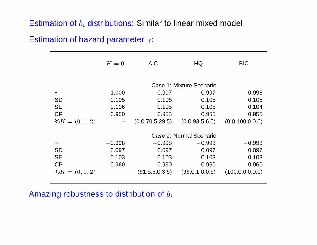
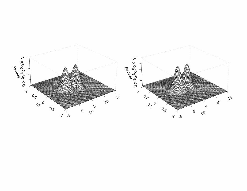
Estimation of bi distributions: Similar to linear mixed model
Estimation of hazard parameter γ:
K = 0 AIC HQ BIC
Case 1: Mixture Scenarioγ −1.000 −0.997 −0.997 −0.996SD 0.105 0.106 0.105 0.105SE 0.106 0.105 0.105 0.104CP 0.950 0.955 0.955 0.955%K = (0, 1, 2) – (0.0,70.5,29.5) (0.0,93.5,6.5) (0.0,100.0,0.0)
Case 2: Normal Scenarioγ −0.998 −0.998 −0.998 −0.998SD 0.097 0.097 0.097 0.097SE 0.103 0.103 0.103 0.103CP 0.960 0.960 0.960 0.960%K = (0, 1, 2) – (91.5,5.0,3.5) (99.0,1.0,0.5) (100.0,0.0,0.0)
Amazing robustness to distribution of bi
-5 0
510
15
b0-1
-0.5
0
0.5
1
b1
00.
20.4
0.6
0.8
1de
nsity
-5 0
510
15
b0-1
-0.5
0
0.5
1
b1
00.
20.4
0.6
0.8
1de
nsity
b0
dens
ity
-5 0 5 10 15
0.0
0.10
0.20
0.30
b1
dens
ity
-1.0 -0.5 0.0 0.5 1.0
01
23
45
−5 0 5 10 15
0.0
0.10
0.20
0.30
b0
dens
ity
−1.0 −0.5 0.0 0.5 1.0
01
23
45
b1
dens
ity
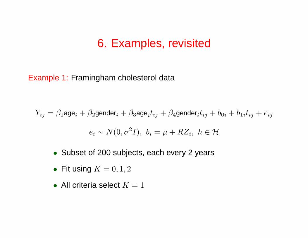
6. Examples, revisited
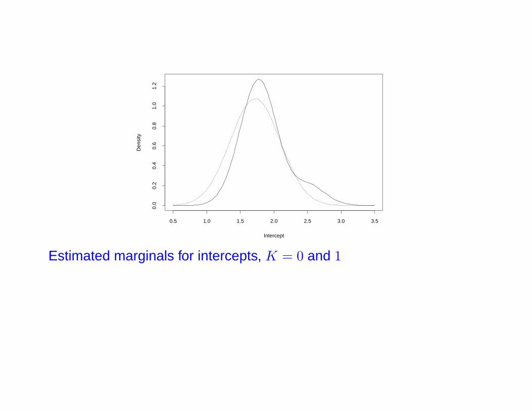
Example 1: Framingham cholesterol data
Yij = β1agei + β2genderi + β3ageitij + β4genderitij + b0i + b1itij + eij
ei ∼ N(0, σ2I), bi = µ+RZi, h ∈ H
• Subset of 200 subjects, each every 2 years
• Fit using K = 0, 1, 2
• All criteria select K = 1
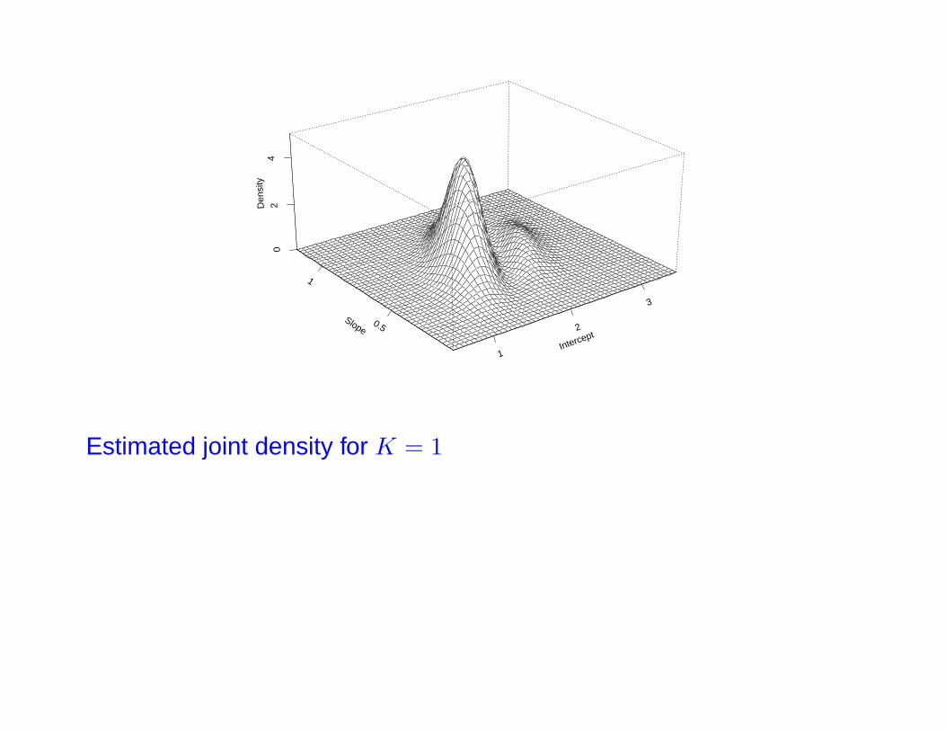
1
2
3
Intercept0.5
1
Slope
02
4D
ensi
ty
Estimated joint density for K = 1
Intercept
Den
sity
0.5 1.0 1.5 2.0 2.5 3.0 3.5
0.0
0.2
0.4
0.6
0.8
1.0
1.2
Estimated marginals for intercepts, K = 0 and 1

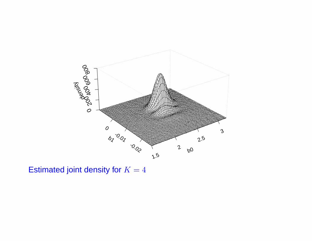
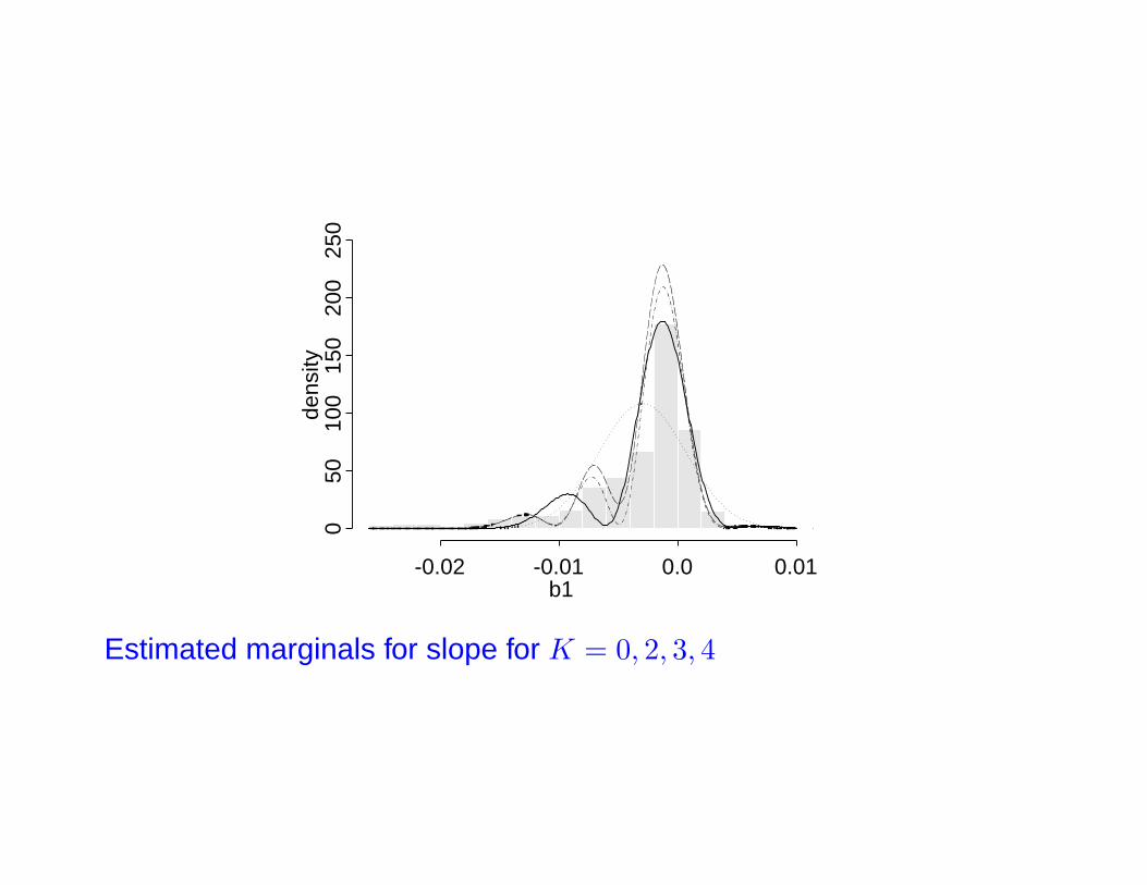
Example 3: ACTG 175 joint longitudinal-survival model
Wij = Xi(tij) + eij, Xi(u) = b0i + b1iu, ei ∼ N(0, σ2)
bi = µ0(1− Si) + µ1Si +RZi, Si = I(Trt=ZDV) h ∈ H,
λi(u) = limdu→0
du−1Pu ≤ Ti < u+ du|Ti ≥ u, αi, Si, Ci, ei, ti
= λ0(u) expγXi(u) + ηTSi
• 2467 subjects
• Fit for K = 0, 1, 2, 3, 4; K = 3 or 4 chosen
1.5
22.5
3
b0-0.02
-0.01
0
b1
020
040
060
080
0de
nsity
Estimated joint density for K = 4
-0.02 -0.01 0.0 0.01
050
100
150
200
250
b1
dens
ity
Estimated marginals for slope for K = 0, 2, 3, 4
7. Discussion
• Potential to gain efficiency in parameters associatedwith subject-level covariates in longitudinal models; otherparameters robust
• Remarkable robustness of inference on hazard parameters tomisspecification of random effects distribution in joint model
• Insight on population heterogeneity, possible omitted covariates
• Implementation only mildly more difficult than assumingnormal random effects