Differentiating between mixed-effects and latent-curveapproaches to growth modeling

Daniel McNeish1& Tyler Matta2

Published online: 24 October 2017# Psychonomic Society, Inc. 2017

Abstract In psychology, mixed-effects models and latent-curve models are both widely used to explore growth overtime. Despite this widespread popularity, some confusion re-mains regarding the overlap of these different approaches.Recent articles have shown that the two modeling frameworksare mathematically equivalent in many cases, which is ofteninterpreted to mean that one’s choice of modeling frameworkis merely a matter of personal preference. However, someimportant differences in estimation and specification can leadto the models producing very different results when imple-mented in software. Thus, mathematical equivalence doesnot necessarily equate to practical equivalence in all cases.In this article, we discuss these two common approaches togrowth modeling and highlight contexts in which the choiceof the modeling framework (and, consequently, the software)can directly impact the model estimates, or in which certainanalyses can be facilitated in one framework over the other.We show that, unless the data are pristine, with a large samplesize, linear or polynomial growth, and no missing data, andunless the participants have the same number of measure-

ments collected at the same set of time points, one frameworkis often more advantageous to adopt. We provide several em-pirical examples to illustrate these situations, as well as amplesoftware code so that researchers can make informed deci-sions regarding which framework will be the most beneficialand most straightforward for their research interests.

Keywords Mixed effect model . Latent growthmodel .

Multilevel model . Hierarchical linearmodel . Structuralequationmodeling

In psychology, empirical questions concerned with changeover time are ubiquitous. As such, statistical methods formodeling longitudinal data concomitant with such questionshave become widely studied in the methodological literature.For modeling growth, researchers typically employ some typeof random effects model such that a mean growth trajectory isestimated for all observations in the data but a unique growthcurve is estimated for each individual in the data as well(Curran & Bauer, 2011). These types of models are generallyreferred to as subject-specific models (Zeger, Liang, & Albert,1988), which are more commonly known in psychology asgrowth curve models. Growth models have many aliases butcan be broadly grouped into two different classes of methods:the latent-curve (LC) approach, which treats the repeated mea-sures as multivariate (also known as the “wide” data format)and tends to be fit with general structural equation modeling(SEM) software (Meredith & Tisak, 1990; Tucker, 1958;Willett & Sayer, 1994), and the mixed-effect (ME) approach,which treats the repeated measures as univariate (also knownas the “long” data format) and is generally fitted with

Electronic supplementary material The online version of this article(https://doi.org/10.3758/s13428-017-0976-5) contains supplementarymaterial, which is available to authorized users.

* Daniel McNeishdmcneish@asu.edu

1 Department of Psychology, Arizona State University, PO Box871104, Tempe, AZ 85287, USA

2 Centre for Educational Measurement, University of Oslo,Oslo, Norway

Behav Res (2018) 50:1398–1414DOI 10.3758/s13428-017-0976-5

regression software (Bryk & Raudenbush, 1987; Laird &Ware, 1982; Rao 1965).1

Over the past 20 years, methodological research has shownthat the LC and ME approaches are actually nuanced twists onthe same idea; they have been shown to converge, and to bemathematically equivalent in many cases (e.g., Bauer, 2003;Curran, 2003; Ledermann & Kenny, 2017; Mehta & Neale,2005). Skrondal and Rabe-Hesketh (2004) went so far as topropose a general latent-variable modeling framework that ef-fectively unified the LC and ME approaches. Historically, thetreatment of this topic has focused on conditions for which thetwo growth-modeling frameworks converge. Bauer (2003) andCurran (2003) showed types of models for which the parame-ters in one framework mapped directly onto the parameters inthe other. Chou, Bentler, and Pentz (1998) demonstrated thatidentical results can be obtained in either framework undercertain conditions. Convergence has been shown similarly inthe cases of missing data (Ferrer, Hamagami, & McArdle,2004), interaction tests (Preacher, Curran, & Bauer, 2006),and subject-specific estimates (Mehta & West, 2000). Clearly,there is much overlap between the two modeling frameworks.

Although certainly there is a notable mathematical similaritybetween the LC and ME approaches, they are not alwaysidentical, and there remains confusion regarding whendivergence occurs. We believe that this ambiguity does not liein the mathematical model but is largely a result of softwareimplementation, whereby some extensions are made easierunder LC software, whereas others are more straightforwardunder the ME software. However, the recent literature has losttrack of the extent to which the overlap extends, often resultingin claims that the modeling frameworks will produce identicalresults. For example, Hox (2010) states that “when equivalentmultilevel regression analysis and latent curve modeling areapplied to the same data set, the results are identical” (p. 243).

There is indeed much overlap between the frameworks, andestimates from both frameworks indeed do converge, givenideal data. However, in empirical studies, in which the dataare often nonnormal or missing, are collected at nonuniformintervals, or have small samples, nontrivial differences betweenthe frameworks will result in different conclusions, or at least ina varying difficulty with which the models can be fit. The goalof this article is to provide a clear overview of the LC and MEapproaches to growth curve analysis and to highlight wherethese two approaches differ practically, rather thantheoretically. We highlight some of the major differences inthe implementation of these models in commonly used

statistical software, and include demonstrations of the differ-ences via empirical examples. We conclude by offering a sum-mary of the situations in which the methods are not equallyadvantageous to implement, and we provide recommendationsregarding when each framework may provide particular advan-tages for empirical researchers fitting models to data. Thus,even though some studies have demonstrated the broad conver-gence of growth modeling frameworks, we feel that it is impor-tant to also demonstrate their meaningful divergence, as well.

Overview of the mixed-effect approach

The ME approach accounts for the fact that individuals aremeasured repeatedly over time by modeling the intercept and/or the time coefficients as random (Laird & Ware, 1982;Stiratelli, Laird, & Ware, 1984). This allows researchers toestimate a mean trajectory for the entire sample, as well assubject-specific deviations from the mean for each person inthe data. The mean trajectory parameters for the whole sampleare commonly referred to as “fixed effects.” These fixed ef-fects—which are most commonly the intercept, time (and anyfunctions thereof, such as polynomial terms), and any time-varying covariates—can also be included in the random-effects portion of the model. Random effects capture howmuch the estimates for a particular person differ from thefixed-effect estimate, which allows the growth trajectory todiffer for each person.

More formally, with continuous outcomes, the linear MEmodel can be written in Laird and Ware’s (1982) notation as

yi ¼ Xiβþ Ziui þ εi; ð1Þ

where yi is an mi × 1 vector of responses for person i, mi is thenumber of observations for person i, Xi is an mi × p designmatrix for the predictors in person i, p is the number of predic-tors (which includes the intercept), β is a p × 1 vector of fixedregression coefficients, Zi is an mi × r design matrix for therandom effects of person i, r is the number of random effects,ui is an r × 1 vector of random effects for person i, where ui ~MVN(0,G), and εi is a matrix of residuals of the observationsin person i, where εi ~ MVN(0, Ri) and Cov(ui, εi) = 0.

As an alternative to the Laird and Ware (1982) matrix no-tation in Eq. 1, it is common in behavioral science literaturesto see ME models written in Raudenbush and Bryk (2002;hereafter, RB) notation, as well. In RB notation, Eq. 1 canbe written as

Y ij ¼ β0i þ β1iTimeij þ rij;β0i ¼ γ00 þ γ01X 1i þ…þ γ0kX ki þ u0i;β1i ¼ γ10 þ γ11X 1i þ…þ γ1kX ki þ u1i;

ð2Þ

1 We adopt the ME and LC set of terminology advanced by Cudeck (1996),which was one of the first articles to contrast these methods, to differentiatebetween these two frameworks. However, we recognize that these analyticalapproaches carry many different monikers. For example, Skrondal and Rabe-Hesketh (2004) refer to these exact same approaches as factor models andrandom coefficient models, while Curran (2003) uses the terms multilevelmodel and structural equation model.

Behav Res (2018) 50:1398–1414 1399

where Yij is the response for the ith person at the jth time, β0i isthe intercept for the ith person, β1i is the slope for the ithperson, γ are fixed-effect parameters that do not have an isubscript because they are constant for all people, ui = (u0i,u1i)

T is a vector of random effects for the ith person, Timeij isthe jth time point for the ith person, and rij is the residual forthe ith person at the jth time. The covariance matrix for therandom effects (u) is often represented by T rather than G inthis notation. Similarly, the covariance matrix of the residuals(r) are represented by V rather than R.

Popular software programs used to fit linear ME modelsinclude, but are not limited to, SAS Proc Mixed, SPSSMIXED, Stata xtmixed, the lme4 package in R, and theHLM software program.

Overview of the latent-curve approach

The LC approach for growth essentially follows the samepremise as ME models, except that growth is formulated ina general SEM framework rather than as an extension ofthe regression framework. Specifically, LC models areconfirmatory factor analysis (CFA) models with an im-posed factor mean structure and particular constraints toyield estimates of growth. The basic idea of the LC frame-work for growth is identical to that of the ME framework—there is some overall mean trajectory for the entire sample,but each individual receives random-effect estimate(s) tocapture how their particular growth curve differs from theoverall trajectory. The main conceptual difference is thatthe random effects are specified as latent variables in aCFA, rather than as randomly varying regression coeffi-cients; however, these two notions can be shown to bemathematically equivalent (see, e.g., Curran, 2003).

In SEMmatrix notation, the LCmodel for growth is writtenas

Yi ¼ Λ ηi þ εi;ηi ¼ α þ ΓXi þ ζi;

ð3Þ

where Λ is a matrix of factor loadings that can be, but arenot always, prespecified to fit a specific type of growthtrajectory; ηi is a vector of subject-specific growth factor(intercept and slope) values for person i; εi is a vector ofresiduals for person i, which are distributed MVN(0,Θ); αis a vector of growth factor means; Γ is a matrix of coef-ficients for the predicted effect of time-invariant covariateson the latent growth trajectory factors; Xi is a matrix oftime-invariant covariates for person i; and ζi is a vectorof random effects for person i and is distributed MVN(0,Ψ). Figure 1 shows a path diagram of a hypothetical un-conditional (i.e., no covariates) LC model with four timepoints and the values of Λ constrained to feature linear

growth. Software commonly used to fit growth models inthe LC framework includes Mplus, LISREL, AMOS, thelavaan R package, and SAS Proc Calis.

A brief comparison of the ME and LC approaches

As has been well-explained (e.g., Curran, 2003; Singer &Willett, 2003; Skrondal & Rabe-Hesketh, 2004), the ME ap-proach has much in common with the LC approach.Comparing Eq. 2 to Eq. 3,

& α and Γ are related to γ,& Ψ is related to T,& ηi is related to βi,& Θ is related to V.

To highlight the similarity between the ME and LC equa-tions, in the case in which each person is measured at the sametime points (a.k.a. time-structured data), the matrix expressionin Eq. 3 simplifies to

Y ij ¼ η0i þ η1iTimej þ εij;η0i ¼ αβ0 þ γ01X 1i þ…þ γ0kX ki þ ζ0i;η1i ¼ αβ1 þ γ11X 1i þ…þ γ1kX ki þ ζ1i;

ð4Þ

where Yij is the response for the ith person at the jth time,η0i is the latent intercept for the ith person, η1i is the latentslope for the ith person, γ are the paths from time-invariantpredictors, ζi = (ζ0i, ζ1i)

T is a vector of random effects forthe ith person, Timej is the jth time point, and εij is theresidual for the ith person at the jth time. Without muchexamination, it can be seen that Eq. 4 is essentially identi-cal to Eq. 2, except for the different parameter labels aris-ing from a different modeling framework. The equivalence

Fig. 1 Hypothetical latent growth model path diagram with four timepoints and linear growth. Numeric values indicate parameters that areconstrained. Y indicates the observed variable values at each time point,η are growth factors, ψ are the disturbance co/variances of the latentgrowth parameters, α are the latent factor means, and ε are residuals(whose unlabeled variances would be θ)

1400 Behav Res (2018) 50:1398–1414

between the ME and LC frameworks, both mathematicaland functional, however, is not perfect.

Differences in implementation

Prior to delving into specific details about the key differencesbetween the implementations of the ME and LC frameworks,Table 1 presents a simplified summary of the arguments thatwill be presented for the remainder of this article, along withrecommendations for which type of model is best suited to dealwith particular scenarios. These recommendations are not de-finitive, because they assume that each situation is to be accom-modated in isolation—in reality, it is common for more thanone of these conditions to be present in a single analysis (e.g.,multigroup analysis of nonlinear growth with a small samplesize). In such cases, there may not be a perfect solution toadequately model all facets of the data in question, soresearchers may need to weigh the pros and cons of each ofthe frameworks. These recommendations also apply

predominantly to continuous outcomes, and different recom-mendations may be desirable in the presence of discrete out-come variables.

To generally summarize Table 1, the ME approach tends tobe most useful for straightforward models (e.g., a simplegrowth trajectory with one outcome variable), with complexdata structures such as smaller samples, time-unstructured da-ta, or multiple levels of nesting requiring more flexibility.Conversely, the LC approach is best suited to complex modelswith straightforward data structures, such as growth modelsembedded in larger models, assessments of global model fit,unconstrained time-varying covariates, and complex variancefunctions. Elaboration of these issues will be the focus of theremainder of this article. SAS and Mplus code from the sub-sequent examples is provided in an online supplement.

Small sample sizes

Although a smaller sample size does not alter the mathemat-ical equivalence of the models, it does affect the estimation

Table 1 Summary of recommendations for choosing between ME and LC frameworks in practice

Context Summary and Recommendation

Small samples The ME approach offers more options to accommodate growth models with few people. Bayesian methods arealluring in the LC framework, although researchers must be especially careful with the prior distributions.

Time-unstructured data The ME approach minimally distinguishes between time-structured and time-unstructured data with respect tosoftware implementation. The LC approach is viable with time-unstructured data in most cases, provided thatspecific conditions are met and additional steps are taken.

Nonlinear growth If researchers know that growth will be nonlinear but are not concerned with or do not know the particular function,the latent-basis model in the LC approach offers an easy option that yields a straightforward interpretation. Forspecific forms of nonlinear growth, the ME approach should be preferred, because it can estimate the modeldirectly and does not need to linearize the model prior to estimation, as is needed in structured LC models.

Multiple-group models Either framework can accommodate multigroup models as they are commonly applied. If partial constraints aredesired, the LC framework is far more flexible and can more easily accommodate situations in which a specificsubset of parameters should be constrained or freely estimated.

Model fit Global model fitting is a unique advantage of the LC framework. Researchers should be judicious about the indicesthey report and should keep in mind that growthmodels in an LC framework have an implied-mean structure (e.g.,SRMR tends to perform poorly). Researchers should also be mindful that these criteria can perform undesirablywith small samples, if uncorrected.

Residual structures Differences between the frameworks are fairly minor. The LC framework is more flexible but requires all relations tobe manually programmed or constrained. The ME framework simplifies the process with preprogrammedstructures but is less flexible.

Three-level models Three-level random-effects models are a natural extension of the ME framework and present no difficulty. Athree-level random-effects model is quite difficult to fit in the LC framework, but if the third level is treated with afixed-effects approach, then three levels are no more difficult to fit than a standard LC model.

Growth model embedded in alarger model

Embedding a growth model within a larger model or extending a growth model beyond linear growth with observedvariables is straightforward to do in an LC framework. Options exist in the ME framework, as well, but to variousdegrees can be difficult to program.

Missing data MostME software will listwise delete observations with missing predictors, because the likelihood is conditional. LCsoftware can accommodate missing predictors with FIML because the joint likelihood is typically used. Softwarefor either framework can impute missing values.

Time-varying covariates The ME framework constrains the effect to be constant across all time points and constrains the correlation betweenthe covariate and the growth factors to be 0. These constraints can be lifted in the LC framework. Both frameworksallow for random effects of time-varying covariates.

Behav Res (2018) 50:1398–1414 1401

options that researchers have at their disposal (McNeish,2016b). Methodological research on clustered data in general(of which growth models form a subset) has shown that fullmaximum likelihood estimation leads to downwardly biasedestimates of random-effect variances, fixed-effect standard er-rors, and growth factor mean standard errors when a studyincludes fewer than about 50 people (e.g., W. J. Browne &Draper, 2006; McNeish & Stapleton, 2016). This underesti-mates the variability in individual growth curves and can vast-ly inflate the operating Type I error rate of time-invariant pre-dictors and growth factor means. However, full maximumlikelihood is the primary frequentist method by which modelsin the LC framework are estimated. Robust estimation basedon Huber–White so-called sandwich estimators also does notsolve the issue pertaining to standard error estimation withsmall sample sizes (Maas & Hox, 2004).

In the ME framework, this issue has been well-studied andhas largely been addressed via restricted maximum likelihoodestimation (REML) to address the bias in the random-effectvariances (Harville, 1977), and Kenward–Roger correction toaddress the bias in standard error estimates and inflated oper-ating Type I error rates (Kenward & Roger, 1997, 2009).Recent studies have shown that these methods perform wellwith sample sizes as low as the single digits if reasonablemodel complexity is observed (Ferron, Bell, Hess, Rendina-Gobioff, & Hibbard, 2009). Unfortunately, as has been notedin McNeish (2016a), these methods do not have analogues inthe LC framework,2 and small-sample issues continue to bevastly underresearched in the LC as compared to the MEframework. McNeish (2016b) discusses in full detail the dif-ficulty of deriving a REML-type estimator for the LC frame-work. Without delving into these details, the general issue isthat the restricted likelihood function involves additional com-putations that are manipulations of the fixed-effect design ma-trix (X in Eq. 1). This matrix does not exist in the LC frame-work, because its elements are allocated to the α, Λ, and Xmatrices in Eq. 3. Additionally, as will be discussed shortly,the freedomwithin the LC approach allows the elements in theΛ matrix to be estimated (in the ME framework these ele-ments are variables, not parameters, and cannot be estimated),which further complicates the derivation of a broadly applica-ble REML-type estimator in the LC framework.

Furthermore, different test statistics are utilized in eachframework. In the SEM software programs used in the LCapproach, parameters are tested with Z or χ2 statistics. In MEsoftware programs, the fixed-effect parameters are tested with tor F statistics, which are more appropriate with smaller samplesizes, because they do not assume infinite denominator degrees

of freedom, as is the case with the Z or χ2 statistic (however,the appropriate degrees of freedom for such tests are widelydebated; see, e.g., Schaalje, McBride, & Fellingham, 2002).Although it is known that the Z distribution is the limitingdistribution of the t distribution, and similarly that χ2 is thelimiting distribution of the F distribution, using asymptotic teststatistics with smaller samples can artificially inflate the oper-ating Type I error rate, even if all parameters are estimatedwithout bias (e.g., Schaalje et al., 2002).

Although small-sample-size issues may seem somewhattrivial, small-sample inference is an increased priority ingrowth models, because of the data collection difficulties inmany contexts. That is, longitudinal data are difficult and ex-pensive to collect, and meta-analytic reviews have shown thatabout one-third of growth model studies feature sample sizesin the double or single digits (e.g., Roberts & DelVecchio,2000). McNeish (2016a) further went on to show thatBayesian estimation of small-sample LC growth models (aleading alternative to REML) does not necessarily alleviatethese small-sample concerns, unless careful consideration isgiven to the prior distributions (see van de Schoot, Broere,Perryck, Zondervan-Zwijnenburg, & van Loey, 2015, for spe-cifics on setting the prior distributions for small-samplegrowth models), and also showed that small-sample methodsdeveloped in the ME context can yield estimates superior tothose in the LC context with uninformative prior distributions.

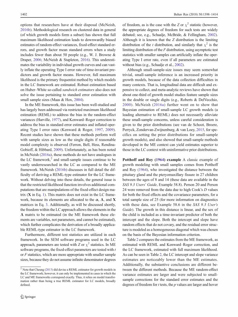
Potthoff and Roy (1964) example A classic example ofgrowth modeling with small samples comes from Potthoffand Roy (1964), who investigated the distance between thepituitary gland and the pteryomaxillary fissure in 27 childrenbetween the ages of 8 and 14 (these data are available in theSAS 9.3 Users’ Guide, Example 58.8). Person 20 and Person24 were removed from the data due to high Cook’s D valuesfor both the fixed effects and the covariance parameters, for atotal sample size of 25 (for more information on diagnosticswith these data, see Example 58.6 in the SAS 9.3 User’sGuide). The growth in this distance is linear, and the sex ofthe child is included as a time-invariant predictor of both theintercept and the slope. Both the intercept and slope haverandom effects that do not covary, and the residual error struc-ture is modeled as a homogeneous diagonal which was chosenon the basis of the Bayesian information criterion.

Table 2 compares the estimates from theME framework, asestimated with REML and Kenward–Roger correction, andthe LC framework, estimated with full maximum likelihood.As can be seen in Table 2, the LC intercept and slope varianceestimates are noticeably lower than the ME estimates.Additionally, the substantive conclusions are different be-tween the different methods. Because the ME random-effectvariance estimates are larger and were subjected to small-sample corrections for the standard error estimates and thedegrees of freedom for t tests, the p values are larger and hover

2 Note that Cheung (2013) did devise a REML estimator for growth models inthe LC framework; however, it can only be implemented in cases in which theLC and ME frameworks correspond exactly. Thus, it relies on model transfor-mation rather than being a true REML estimator for LC models, broadlydefined.

1402 Behav Res (2018) 50:1398–1414

right around the .05 mark. On the other hand, the p valuesassociated with the LC estimates are based on standard errorestimates that are known to be downwardly biased while alsousing a questionably appropriate asymptotic sampling distri-bution, and therefore they are clearly under .05 with thesedata. Granted, the change in statistical significance is a nuanceof these particular data and will not be universal. However, itserves to highlight that, despite identical coefficient estimates,the variance and standard errors are estimated differently be-tween the frameworks with smaller samples.

Time-unstructured data

Longitudinal research designs are often thought of asmultiwave, time-structured studies, meaning that all subjectsprovide a measure at the same time or at every wave.Nonetheless, practically speaking, data commonly deviatefrom the time-structured format (Singer & Willett, 2003;Sterba, 2014). When people in a longitudinal study are mea-sured at different time points, the data are referred to as time-unstructured, which can be especially common when the timevariable of interest is chronological age (especially in youngerchildren, with whom it is important to record age to the monthrather than the year). Because time is most often thought of ascontinuous, coarsening it by treating time as equivalent for allpeople when it is not can have an adverse impact on the pa-rameter estimates (Aydin, Leite, & Algina, 2014; Singer &Willett, 2003). The degree to which this coarsening will im-pact estimates depends on how variably spaced the measure-ment occasions are (Coulombe, Selig, & Delaney, 2016;Singer & Willett, 2003).

Because the ME framework processes data in the “long,”univariate format and Time is an explicit predictor in the mod-el, variably spaced measurement occasions and varying num-bers of measurement occasions do not present a challenge(McCoach, Rambo, & Welsh, 2013; Sterba, 2014). That is,

both X and Z in Eq. 1 have an i subscript, indicating that eachsubject has its own values for time. For Eq. 2, which shows theME specification in RB notation, Time has an i subscript,which allows each person to have unique time values in thedata. In contrast, the LC framework processes datamultivariately, meaning that each time point requires a uniquecolumn in the data (i.e., SEM software requires data to be inthe “wide” format). That is, Λ in Eq. 3 does not have an isubscript, indicating that all subjects are expected to have thesame time values. With time-unstructured data in which eachperson has potentially unique time points, structuring the datain the LC framework can become problematic.

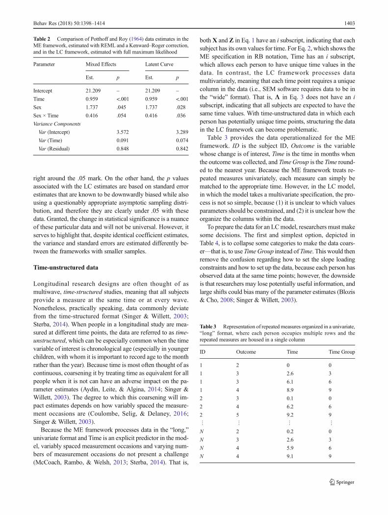
Table 3 provides the data operationalized for the MEframework. ID is the subject ID, Outcome is the variablewhose change is of interest, Time is the time in months whenthe outcome was collected, and Time Group is the Time round-ed to the nearest year. Because the ME framework treats re-peated measures univariately, each measure can simply bematched to the appropriate time. However, in the LC model,in which the model takes a multivariate specification, the pro-cess is not so simple, because (1) it is unclear to which valuesparameters should be constrained, and (2) it is unclear how theorganize the columns within the data.

To prepare the data for an LCmodel, researchers must makesome decisions. The first and simplest option, depicted inTable 4, is to collapse some categories to make the data coars-er—that is, to use TimeGroup instead ofTime. This would thenremove the confusion regarding how to set the slope loadingconstraints and how to set up the data, because each person hasobserved data at the same time points; however, the downsideis that researchers may lose potentially useful information, andlarge shifts could bias many of the parameter estimates (Blozis& Cho, 2008; Singer & Willett, 2003).

Table 2 Comparison of Potthoff and Roy (1964) data estimates in theME framework, estimated with REML and a Kenward–Roger correction,and in the LC framework, estimated with full maximum likelihood

Parameter Mixed Effects Latent Curve

Est. p Est. p

Intercept 21.209 – 21.209 –

Time 0.959 <.001 0.959 <.001

Sex 1.737 .045 1.737 .028

Sex × Time 0.416 .054 0.416 .036

Variance Components

Var (Intercept) 3.572 3.289

Var (Time) 0.091 0.074

Var (Residual) 0.848 0.842

Table 3 Representation of repeated measures organized in a univariate,“long” format, where each person occupies multiple rows and therepeated measures are housed in a single column

ID Outcome Time Time Group

1 2 0 0

1 3 2.6 3

1 3 6.1 6

1 4 8.9 9

2 3 0.1 0

2 4 6.2 6

2 5 9.2 9

⋮ ⋮ ⋮ ⋮N 2 0.2 0

N 3 2.6 3

N 4 5.9 6

N 4 9.1 9

Behav Res (2018) 50:1398–1414 1403

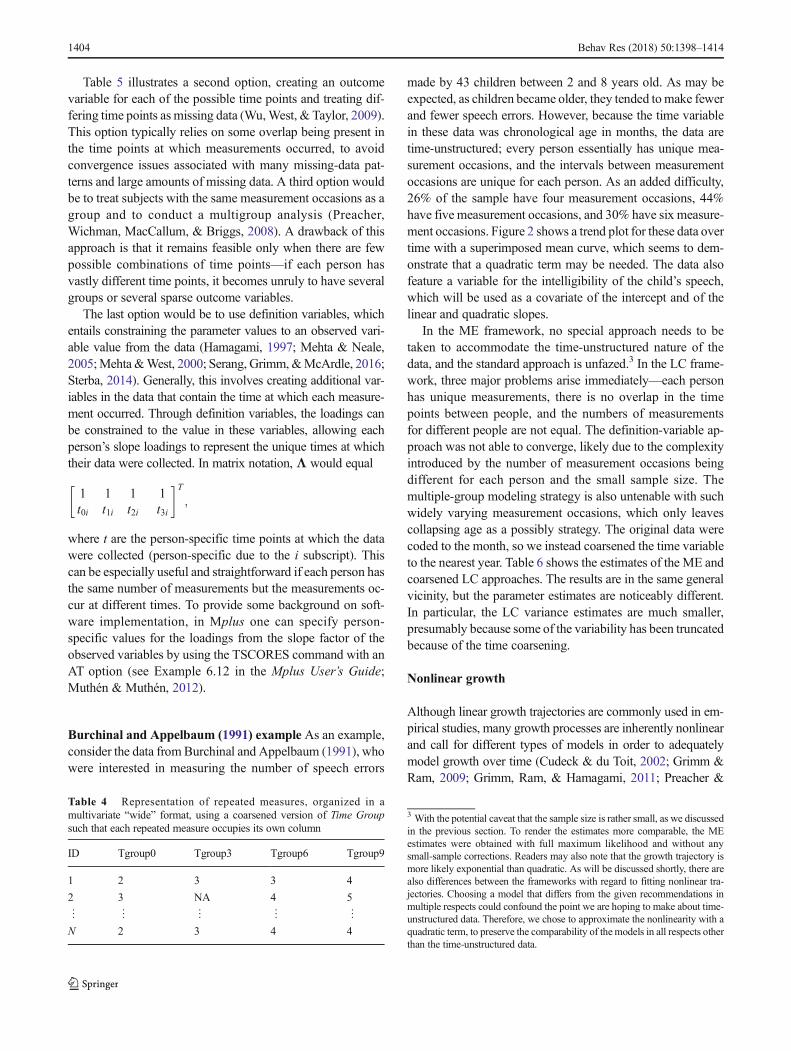
Table 5 illustrates a second option, creating an outcomevariable for each of the possible time points and treating dif-fering time points as missing data (Wu,West, & Taylor, 2009).This option typically relies on some overlap being present inthe time points at which measurements occurred, to avoidconvergence issues associated with many missing-data pat-terns and large amounts of missing data. A third option wouldbe to treat subjects with the same measurement occasions as agroup and to conduct a multigroup analysis (Preacher,Wichman, MacCallum, & Briggs, 2008). A drawback of thisapproach is that it remains feasible only when there are fewpossible combinations of time points—if each person hasvastly different time points, it becomes unruly to have severalgroups or several sparse outcome variables.

The last option would be to use definition variables, whichentails constraining the parameter values to an observed vari-able value from the data (Hamagami, 1997; Mehta & Neale,2005;Mehta&West, 2000; Serang, Grimm,&McArdle, 2016;Sterba, 2014). Generally, this involves creating additional var-iables in the data that contain the time at which each measure-ment occurred. Through definition variables, the loadings canbe constrained to the value in these variables, allowing eachperson’s slope loadings to represent the unique times at whichtheir data were collected. In matrix notation, Λ would equal

1 1 1t0i t1i t2i

1t3i

� �T;

where t are the person-specific time points at which the datawere collected (person-specific due to the i subscript). Thiscan be especially useful and straightforward if each person hasthe same number of measurements but the measurements oc-cur at different times. To provide some background on soft-ware implementation, in Mplus one can specify person-specific values for the loadings from the slope factor of theobserved variables by using the TSCORES command with anAT option (see Example 6.12 in the Mplus User’s Guide;Muthén & Muthén, 2012).

Burchinal and Appelbaum (1991) example As an example,consider the data fromBurchinal and Appelbaum (1991), whowere interested in measuring the number of speech errors

made by 43 children between 2 and 8 years old. As may beexpected, as children became older, they tended tomake fewerand fewer speech errors. However, because the time variablein these data was chronological age in months, the data aretime-unstructured; every person essentially has unique mea-surement occasions, and the intervals between measurementoccasions are unique for each person. As an added difficulty,26% of the sample have four measurement occasions, 44%have five measurement occasions, and 30% have six measure-ment occasions. Figure 2 shows a trend plot for these data overtime with a superimposed mean curve, which seems to dem-onstrate that a quadratic term may be needed. The data alsofeature a variable for the intelligibility of the child’s speech,which will be used as a covariate of the intercept and of thelinear and quadratic slopes.

In the ME framework, no special approach needs to betaken to accommodate the time-unstructured nature of thedata, and the standard approach is unfazed.3 In the LC frame-work, three major problems arise immediately—each personhas unique measurements, there is no overlap in the timepoints between people, and the numbers of measurementsfor different people are not equal. The definition-variable ap-proach was not able to converge, likely due to the complexityintroduced by the number of measurement occasions beingdifferent for each person and the small sample size. Themultiple-group modeling strategy is also untenable with suchwidely varying measurement occasions, which only leavescollapsing age as a possibly strategy. The original data werecoded to the month, so we instead coarsened the time variableto the nearest year. Table 6 shows the estimates of the ME andcoarsened LC approaches. The results are in the same generalvicinity, but the parameter estimates are noticeably different.In particular, the LC variance estimates are much smaller,presumably because some of the variability has been truncatedbecause of the time coarsening.

Nonlinear growth

Although linear growth trajectories are commonly used in em-pirical studies, many growth processes are inherently nonlinearand call for different types of models in order to adequatelymodel growth over time (Cudeck & du Toit, 2002; Grimm &Ram, 2009; Grimm, Ram, & Hamagami, 2011; Preacher &

3 With the potential caveat that the sample size is rather small, as we discussedin the previous section. To render the estimates more comparable, the MEestimates were obtained with full maximum likelihood and without anysmall-sample corrections. Readers may also note that the growth trajectory ismore likely exponential than quadratic. As will be discussed shortly, there arealso differences between the frameworks with regard to fitting nonlinear tra-jectories. Choosing a model that differs from the given recommendations inmultiple respects could confound the point we are hoping to make about time-unstructured data. Therefore, we chose to approximate the nonlinearity with aquadratic term, to preserve the comparability of themodels in all respects otherthan the time-unstructured data.

Table 4 Representation of repeated measures, organized in amultivariate “wide” format, using a coarsened version of Time Groupsuch that each repeated measure occupies its own column

ID Tgroup0 Tgroup3 Tgroup6 Tgroup9

1 2 3 3 4

2 3 NA 4 5

⋮ ⋮ ⋮ ⋮ ⋮N 2 3 4 4

1404 Behav Res (2018) 50:1398–1414

Hancock, 2015; Sterba, 2014). The estimation and specifica-tion of nonlinear models can be vastly different between theME and LC frameworks, with many different types of modelsbeing uniquely estimable in only one framework. We will notbe able to fully cover all of the nuances of nonlinear models ina single section, since many full-length articles have been ded-icated solely to this topic (e.g., Blozis &Harring, 2016b); how-ever, we will attempt to highlight the most salient of the differ-ences that are likely to arise in empirical research.

A notable difference between the ME and LC frameworksis their ability to handle models with nonlinear parameters. Toexplain, nonlinear models can be nonlinear in their variablesor their parameters. A model with a second-order polynomialterm [e.g., E(Y) = β0 + β1Time + β2Time2] is linear in itsparameters, since the β coefficients only appear after additionsigns, but nonlinear in its variables, because Time enters themodel with a quadratic term. Conversely, an exponentialgrowth model [e.g., E(Y) = αF + (α0 – αF) exp (– αRTime)]is nonlinear in its parameters, because the rate parameter (e.g.,– αR) appears in the exponential expression.

ME software is able to accommodate either of these speci-fications without changing the interpretation of the model

parameters (e.g., SAS ProcMixed for models nonlinear in theirvariables, SAS Proc NLMIXED for models nonlinear in theirparameters; Blozis & Harring, 2016b). SEM software can ac-commodate models that are nonlinear in their variables butcannot directly accommodate models that are nonlinear in theirparameters (Blozis & Harring, 2016b). A common method tofit models that are nonlinear in their parameters using SEMsoftware is through a structured latent-curve model (SLCM;Blozis, 2004; M. W. Browne, 1993), which linearizes the non-linear portions of the model using Taylor series expansions (fordetails on this procedure, see Blozis & Harring, 2016a).Although many consider the SLCM to be the LC equivalentof nonlinear ME models, as detailed by Blozis and Harring(2016b), the linearization process changes the interpretationof the model and of the random effects (the interpretation ofthe factor means takes a population-averaged rather than asubject-specific interpretation, which are not equivalent in non-linear models; Fitzmaurice, Laird, & Ware, 2004; Zeger et al.,1988). In SLCMs, subject-specific curves are not required tofollow the same functional form as the mean curve—the onlyrestriction is that the sum of the subject-specific curves mustequal the mean trajectory. In nonlinear ME models, everysubject-specific curve follows the same functional form as the

Fig. 2 Plot of speech error learning curves for all 43 children in theBurchinal and Appelbaum (1991) data, with a mean curvesuperimposed in black

Table 5 Representation of repeated measures, organized in a multivariate format using the original time metric Time. Notice the large amount ofmissing data, indicated by NA

ID T0 T0.10 T0.20 T2.35 T2.60 T5.90 T6.10 T6.20 T8.90 T9.10 T9.20

1 2 NA NA 3 NA NA 3 NA 4 NA NA

2 NA 3 NA NA NA NA NA 4 NA 5 NA

⋮ ⋮ ⋮ ⋮ ⋮ ⋮ ⋮ ⋮ ⋮ ⋮ ⋮ ⋮N NA NA 2 NA NA 4 NA NA NA NA 4

Table 6 Comparison of model estimates for Burchinal and Appelbaum(1991) data for ME and a LC that coarsens time

Parameter Mixed Effects Coarsened Latent Curve

Est. p Est. p

Intercept 90.32 – 105.78 –

Time – 26.81 <.01 – 30.50 <.01

Time2 2.00 <.01 2.20 <.01

Intelligibility – 7.21 <.01 – 12.39 <.01

Time × Intelligibility 2.04 .02 3.60 .02

Time2 × Intelligibility – 0.15 .07 – 0.26 .04

Variance Components

Var (Intercept) 112.82 91.70

Var (Time) 2.16 1.59

Cov (Intercept, Time) – 15.93 – 12.48

Var (Residual) 20.48 21.73

Behav Res (2018) 50:1398–1414 1405

mean curve—thus, differences between people stem only fromthe subject-specific random-effect estimates, not from poten-tially different trajectories altogether.

An advantage of modeling nonlinear growth in the LCframework is the so-called latent-basis model (McArdle,1986; Meredith & Tisak, 1990) or free curve (Wood &Jackson, 2013). In the LC framework, time is a parameter ofthe model (the values of the loadings from the slope factor)rather than a variable in the data. As a result, one can estimatethe values of these slope loadings rather than fixing them tospecific values. To give the slope factor scale, two loadingsmust be constrained, and a common choice is to constrain theloading of the first time point to 0 and the loading of the lasttime point to 1, while estimating the loadings of all intermediatetime points. When the growth trajectory is specified a priori, foran unconditional linear growthmodel with time-structured data,

Λ ¼ Xi ¼ 1 1 10 1 2

13

� �T:

However, in a latent-basis model,

Λ ¼ 1 1 10 λ21 λ31

11

� �T;

where λ are estimated parameters; this is not feasible to do inlinear ME models, because the elements of Xi are variables inthe data and therefore not estimable. Grimm, Ram, andEstabrook (2016) have noted, however, that the latent-basismodel can be coerced to fit in theME framework as a nonlinearmixed-effect model. They provide code for fitting a latent-basismodel in SAS Proc NLMIXED on their page 243, through theclever use of data steps. This code is restricted to having theresidual variance constrained across time points, however.

With this approach, the slope factor mean is an estimate ofthe amount of total growth that occurs over the entire obser-vation window, provided that the first loading is constrained to0 and the last loading is constrained to 1. In this case, theestimated slope loadings correspond to the percentages ofthe total growth that has occurred up to and including thatspecific time point (e.g., an estimated slope loading of .65 atTime 3 means that the outcome at Time 3 is 65% of the totalgrowth. It does not mean that 65% of the growth process hasoccurred at Time 3, however, unless the curve is monotonic.).4

This approach can be especially advantageous if researchersknow that growth is nonlinear but are not sure or not interested

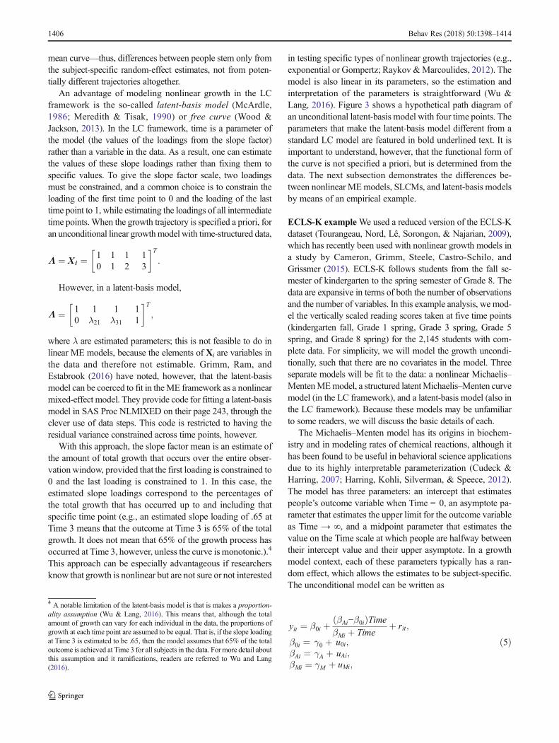
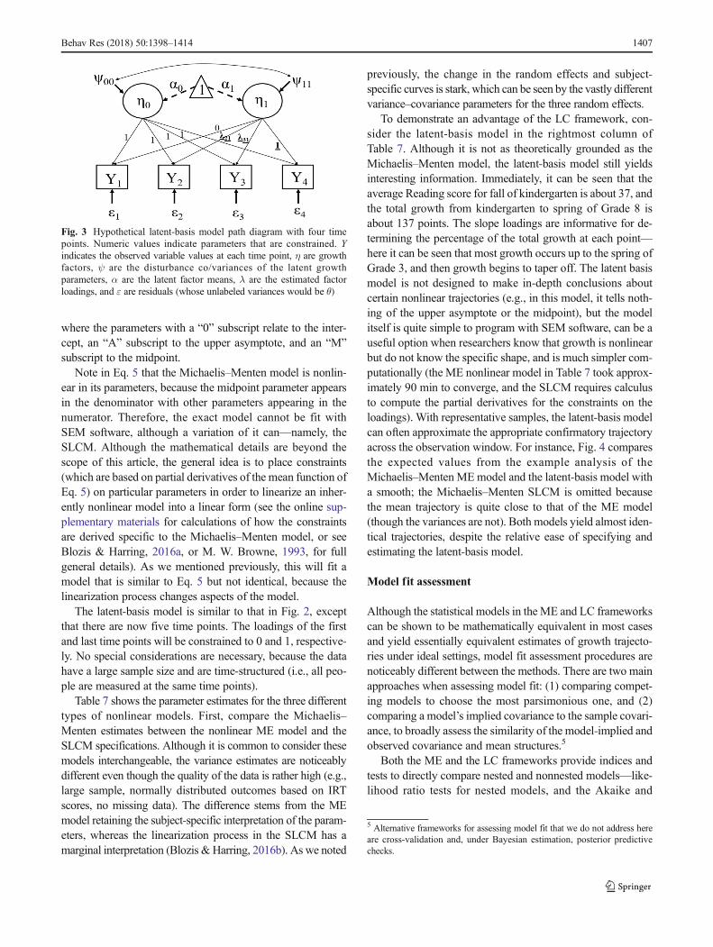
in testing specific types of nonlinear growth trajectories (e.g.,exponential or Gompertz; Raykov &Marcoulides, 2012). Themodel is also linear in its parameters, so the estimation andinterpretation of the parameters is straightforward (Wu &Lang, 2016). Figure 3 shows a hypothetical path diagram ofan unconditional latent-basis model with four time points. Theparameters that make the latent-basis model different from astandard LC model are featured in bold underlined text. It isimportant to understand, however, that the functional form ofthe curve is not specified a priori, but is determined from thedata. The next subsection demonstrates the differences be-tween nonlinear MEmodels, SLCMs, and latent-basis modelsby means of an empirical example.

ECLS-K exampleWe used a reduced version of the ECLS-Kdataset (Tourangeau, Nord, Lê, Sorongon, & Najarian, 2009),which has recently been used with nonlinear growth models ina study by Cameron, Grimm, Steele, Castro-Schilo, andGrissmer (2015). ECLS-K follows students from the fall se-mester of kindergarten to the spring semester of Grade 8. Thedata are expansive in terms of both the number of observationsand the number of variables. In this example analysis, we mod-el the vertically scaled reading scores taken at five time points(kindergarten fall, Grade 1 spring, Grade 3 spring, Grade 5spring, and Grade 8 spring) for the 2,145 students with com-plete data. For simplicity, we will model the growth uncondi-tionally, such that there are no covariates in the model. Threeseparate models will be fit to the data: a nonlinear Michaelis–MentenMEmodel, a structured latentMichaelis–Menten curvemodel (in the LC framework), and a latent-basis model (also inthe LC framework). Because these models may be unfamiliarto some readers, we will discuss the basic details of each.

The Michaelis–Menten model has its origins in biochem-istry and in modeling rates of chemical reactions, although ithas been found to be useful in behavioral science applicationsdue to its highly interpretable parameterization (Cudeck &Harring, 2007; Harring, Kohli, Silverman, & Speece, 2012).The model has three parameters: an intercept that estimatespeople’s outcome variable when Time = 0, an asymptote pa-rameter that estimates the upper limit for the outcome variableas Time → ∞, and a midpoint parameter that estimates thevalue on the Time scale at which people are halfway betweentheir intercept value and their upper asymptote. In a growthmodel context, each of these parameters typically has a ran-dom effect, which allows the estimates to be subject-specific.The unconditional model can be written as

yit ¼ β0i þβAi−β0ið ÞTimeβMi þ Time

þ rit;

β0i ¼ γ0 þ u0i;βAi ¼ γA þ uAi;βMi ¼ γM þ uMi;

ð5Þ

4 A notable limitation of the latent-basis model is that is makes a proportion-ality assumption (Wu & Lang, 2016). This means that, although the totalamount of growth can vary for each individual in the data, the proportions ofgrowth at each time point are assumed to be equal. That is, if the slope loadingat Time 3 is estimated to be .65, then the model assumes that 65% of the totaloutcome is achieved at Time 3 for all subjects in the data. For more detail aboutthis assumption and it ramifications, readers are referred to Wu and Lang(2016).

1406 Behav Res (2018) 50:1398–1414

where the parameters with a “0” subscript relate to the inter-cept, an “A” subscript to the upper asymptote, and an “M”subscript to the midpoint.

Note in Eq. 5 that the Michaelis–Menten model is nonlin-ear in its parameters, because the midpoint parameter appearsin the denominator with other parameters appearing in thenumerator. Therefore, the exact model cannot be fit withSEM software, although a variation of it can—namely, theSLCM. Although the mathematical details are beyond thescope of this article, the general idea is to place constraints(which are based on partial derivatives of the mean function ofEq. 5) on particular parameters in order to linearize an inher-ently nonlinear model into a linear form (see the online sup-plementary materials for calculations of how the constraintsare derived specific to the Michaelis–Menten model, or seeBlozis & Harring, 2016a, or M. W. Browne, 1993, for fullgeneral details). As we mentioned previously, this will fit amodel that is similar to Eq. 5 but not identical, because thelinearization process changes aspects of the model.

The latent-basis model is similar to that in Fig. 2, exceptthat there are now five time points. The loadings of the firstand last time points will be constrained to 0 and 1, respective-ly. No special considerations are necessary, because the datahave a large sample size and are time-structured (i.e., all peo-ple are measured at the same time points).

Table 7 shows the parameter estimates for the three differenttypes of nonlinear models. First, compare the Michaelis–Menten estimates between the nonlinear ME model and theSLCM specifications. Although it is common to consider thesemodels interchangeable, the variance estimates are noticeablydifferent even though the quality of the data is rather high (e.g.,large sample, normally distributed outcomes based on IRTscores, no missing data). The difference stems from the MEmodel retaining the subject-specific interpretation of the param-eters, whereas the linearization process in the SLCM has amarginal interpretation (Blozis &Harring, 2016b). As we noted

previously, the change in the random effects and subject-specific curves is stark, which can be seen by the vastly differentvariance–covariance parameters for the three random effects.

To demonstrate an advantage of the LC framework, con-sider the latent-basis model in the rightmost column ofTable 7. Although it is not as theoretically grounded as theMichaelis–Menten model, the latent-basis model still yieldsinteresting information. Immediately, it can be seen that theaverage Reading score for fall of kindergarten is about 37, andthe total growth from kindergarten to spring of Grade 8 isabout 137 points. The slope loadings are informative for de-termining the percentage of the total growth at each point—here it can be seen that most growth occurs up to the spring ofGrade 3, and then growth begins to taper off. The latent basismodel is not designed to make in-depth conclusions aboutcertain nonlinear trajectories (e.g., in this model, it tells noth-ing of the upper asymptote or the midpoint), but the modelitself is quite simple to program with SEM software, can be auseful option when researchers know that growth is nonlinearbut do not know the specific shape, and is much simpler com-putationally (the ME nonlinear model in Table 7 took approx-imately 90 min to converge, and the SLCM requires calculusto compute the partial derivatives for the constraints on theloadings). With representative samples, the latent-basis modelcan often approximate the appropriate confirmatory trajectoryacross the observation window. For instance, Fig. 4 comparesthe expected values from the example analysis of theMichaelis–Menten MEmodel and the latent-basis model witha smooth; the Michaelis–Menten SLCM is omitted becausethe mean trajectory is quite close to that of the ME model(though the variances are not). Both models yield almost iden-tical trajectories, despite the relative ease of specifying andestimating the latent-basis model.

Model fit assessment

Although the statistical models in the ME and LC frameworkscan be shown to be mathematically equivalent in most casesand yield essentially equivalent estimates of growth trajecto-ries under ideal settings, model fit assessment procedures arenoticeably different between the methods. There are two mainapproaches when assessing model fit: (1) comparing compet-ing models to choose the most parsimonious one, and (2)comparing a model’s implied covariance to the sample covari-ance, to broadly assess the similarity of the model-implied andobserved covariance and mean structures.5

Both the ME and the LC frameworks provide indices andtests to directly compare nested and nonnested models—like-lihood ratio tests for nested models, and the Akaike and

5 Alternative frameworks for assessing model fit that we do not address hereare cross-validation and, under Bayesian estimation, posterior predictivechecks.

Fig. 3 Hypothetical latent-basis model path diagram with four timepoints. Numeric values indicate parameters that are constrained. Yindicates the observed variable values at each time point, η are growthfactors, ψ are the disturbance co/variances of the latent growthparameters, α are the latent factor means, λ are the estimated factorloadings, and ε are residuals (whose unlabeled variances would be θ)

Behav Res (2018) 50:1398–1414 1407

Bayesian information criteria for nonnested models. If thesame estimation method is used, these quantities will be iden-tical between the frameworks. However, assessing model fitby comparing the sample covariance and model-implied co-variance is much different for the two frameworks. The LCframework has a host of indices and statistical tests that canhelp determine how well the model-implied covariance andmean structure reproduce the sample covariance and samplemeans (Coffman and Millsap, 2006; Chou et al., 1998; Liu,

Rovine, & Molenaar, 2012; Wu et al., 2009). ME models, onthe other hand, can use visual tools to determine how well themodel-implied covariance reflects the sample covariance(Hedeker & Gibbons, 2006), or can use variance-explainedmeasures (Vonesh, Chinchilli, & Pu, 1996; Xu, 2003) or ap-proximate R2 extensions (Edwards, Muller, Wolfinger,Qaqish, & Schabenberger, 2008; Johnson, 2014; Nakagawa& Schielzeth, 2013), but these methods are less commonlyreported and less mainstream than the indices in the LC frame-work. The flexibility of the ME approach often adds to thisdifficulty. For example, formally comparing model-impliedmatrices to observed matrices can be cumbersome for time-unstructured data, and ME R2 methods can be difficult toimplement when random slopes are included, which is com-mon for growth models (e.g., Snijders & Bosker, 1994).

Although the fit indices in the general SEM frameworkhave been well-studied, because LC growth models requireboth the covariance structure and the mean structure, the pro-tocol for assessing fit differs from conventional SEM fit as-sessment strategies and guidelines—namely because mostSEM fit assessment recommendations are based on modelsthat only model the covariance (e.g., CFA models). In LCgrowth models, the commonly reported SRMR index per-forms quite poorly and rarely identifies misfit in the mean

Table 7 Comparison of different frameworks for nonlinear growth

Michaelis–Menten Latent Basis

Mixed Effects Structured Latent Curve Latent Curve

Parameter Est. Est. Parameter Est.

Intercept 36.38 36.35 Intercept Mean 36.77

Asymptote 257.11 258.32 Slope Mean 136.90

Midpoint 4.89 4.87 Loading Kind. Fall 0.00

Loading Grade 1 Spr. 0.33

Covariance Parameters Loading Grade 3 Spr. 0.71

Var (Intercept) 82.98 100.63 Loading Grade 5 Spr. 0.87

Var (Asymptote) 512.17 285.75 Loading Grade 8 Spr. 1.00

Var (Mid-Point) 1.36 2.87

Corr (Int., Asy.) – 0.43 – 0.46 Covariance Parameters

Corr (Int. Mid.) – 0.85 – 0.62 Var (Intercept) 100.63

Corr (Asy., Mid.) 0.02 0.07 Var (Slope) 508.02

Residual Kind. Fall 32.86 0.00 Corr (Int., Slope) 0.02

Residual Grade 1 Spr. 272.23 256.83 Residual Kind. Fall 0.00

Residual Grade 3 Spr. 154.02 153.97 Residual Grade 1 Spr. 233.30

Residual Grade 5 Spr. 88.73 76.50 Residual Grade 3 Spr. 169.65

Residual Grade 8 Spr. 198.94 233.65 Residual Grade 5 Spr. 66.89

Residual Grade 8 Spr. 231.16

The ME model was estimated with Gaussian quadrature with ten quadrature points. The residual error structure was specified to be a heterogeneousdiagonal in all three models. Significance is not reported because the sample size was large. Bold values were constrained and thus not estimated. Theresidual variance in fall of kindergarten was constrained to zero in the models fit in the LC framework in order to avoid a Heywood case, because theestimate was slightly negative

0

20

40

60

80

100

120

140

160

180

200

0 2 4 6 8 10

Rea

din

g S

core

Time Since Start of Kindergarten (in years)

Michaelis-Menten ME

LC Latent Basis

Fig. 4 Comparison of mean trajectories for the Michaelis–Menten ME(black) and LC latent-basis (gray) models

1408 Behav Res (2018) 50:1398–1414

structure portion of the model (Leite & Stapleton, 2011;Wu&West, 2010). This can be concerning because a major part ofany growth model analysis is to report how people are gener-ally changing over time. Additionally, with such relative fitindices as the comparative fit index (CFI) or the Tucker–Lewis index (TLI), the baseline model that is used as a sourceof comparison is inappropriate. Specifically, Widaman andThompson (2003) noted that, in the CFI and TLI formulas,the baseline model must be nested within the analysis model.However, in LC growth models, the standard baseline modelin the software is often the independencemodel, in which eachobserved variable has an estimated variance and the meanstructure (if present) is saturated (Bentler & Bonett, 1980).This independence model is not nested within LC growthmodels, though, making the CFI and TLI models reportedfrom mainstream SEM software inappropriate in the case ofgrowth models. Instead, Widaman and Thompson (2003) rec-ommended the linear latent-growth model with the interceptvariance constrained to zero as an alternative baseline modelthat is nested in the more expansive LC model.

As we noted in an earlier section, small samples are quitecommon in data suitable for growth modeling in general.Small samples not only affect the estimation of parametersin LC models, but also the calculation of data-model fit sta-tistics and indices (Bentler & Yuan, 1999; Herzog &Boomsma, 2009; Kenny & McCoach, 2003; Nevitt &Hancock, 2004). Without belaboring the specific details, thegeneral issue is that, with smaller samples, the maximumlikelihood test statistic (commonly referred to as TML) doesnot follow the appropriate chi-square distribution with theassociated degrees of freedom. As a result, this test statistictends to have vastly deflated p values, which leads to theover-rejection of models even if the models are perfectlyspecified, until the sample size approaches about 100 people(Kenny & McCoach, 2003). Furthermore, because most LCfit indices are based on some manipulation of the chi-squaretest statistic (e.g., RMSEA, CFI, TLI), these indices are alsoaffected and yield unnecessarily unfavorable assessments offit. Fortunately, three different heuristic small-sample correc-tions have been proposed, by Bartlett (1950), Swain (1975),and Yuan (2005), that adjust the chi-square test statistic sothat it more closely approximates the appropriate chi-squaredistribution. Simulation studies have shown that these correc-tions work well in the general context of SEMs (Fouladi,2000; Herzog & Boomsma, 2009; Nevitt & Hancock,2004). A caveat of these small-sample corrections, however,is that they require a complete dataset (e.g., either the datasetmust have no missing observations or the data must havebeen rectangularized with a suitable missing-data method,such as multiple imputation). For a discussion of issues relat-ed to these small-sample corrections with missing data ingrowth models, readers are referred to McNeish andHarring (2017).

Potthoff and Roy (1964) example To demonstrate, werevisited the previous Potthoff and Roy (1964) example,which has 25 participants. With a sample of this size, it isunlikely that the maximum likelihood chi-square test will beoverpowered, and it is therefore the best measure with whichto assess fit. Because the model has few degrees of freedomand a small sample size, the root-mean square error of approx-imation is not desirable to report, either (Kenny, Kaniskan, &McCoach, 2015). Without any correction, the maximum like-lihood test shows that the hypothesis that the model-impliedmean and covariance structures equal the observed mean vec-tor and covariance matrix should be rejected, and we wouldconclude that the model does not fit well, χ2(11) = 23.152, p =.017. However, with a smaller sample this test tends to over-reject well-fitting models. Both the Bartlett- and Yuan-corrected statistics that have been recommended for LCmodels with small samples and complete data show that thenull hypothesis should not be rejected and that the modelprovides a reasonable fit to the data, χ2

Bart(11) = 19.133, p =.059; χ2

Yuan(11) = 19.454, p = .053. Equivalent measures ofglobal fit in the ME framework are not well-developed, andassessing fit in the ME framework is largely relegated to sig-nificance tests of specific parameters or model comparisons(Wu et al., 2009).

Putting it all together

In previous sections we showed how the LC and ME frame-work differed, one facet at a time. This approach was taken forits didactic simplicity, and more advanced readers may notethat the less beneficial framework may still be viable in thesecircumstances, with the aid of some creative programming.However, as we mentioned earlier, multiple facets on whichthe LC and ME frameworks differ can also be present simul-taneously, which can make the selection of the appropriateframework even more crucial, because the programmingtricks required to combat multiple differences simultaneouslycan be unruly.

Consider the data analyzed by Prosser, Rasbash, andGoldstein (1991), appearing in Rabe-Hesketh and Skrondal(2012), of children’s weights (in kilograms) over the firstfew years of their lives. This particular dataset has a smallsample (n = 68), nonlinear growth (babies gain weight rapidlyat first, but weight gains begin to taper off), unstructured time(the Time variable is chronological age, so each child has aunique value), and a multiple-group component (males andfemales typically are different sizes at this stage of develop-ment). We fit the model in the ME framework using SAS ProcMixed with linear and quadratic terms for growth, random butuncorrelated intercepts and linear slopes, and a homogeneousdiagonal error structure. The model was estimated withREML and a Kenward–Roger correction. Because one of

Behav Res (2018) 50:1398–1414 1409

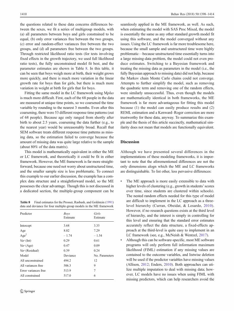
the questions related to these data concerns differences be-tween the sexes, we fit a series of multigroup models, with(a) all parameters between boys and girls constrained to beequal, (b) only error variances free between the two groups,(c) error and random-effect variances free between the twogroups, and (d) all parameters free between the two groups.Through restricted likelihood ratio tests (for tests involvingfixed effects in the growth trajectory, we used full likelihoodratio tests), the fully unconstrained model fit best, and theparameter estimates are shown in Table 8. In this table, itcan be seen that boys weigh more at birth, their weight growsmore quickly, and there is much more variation in the lineargrowth rate for boys than for girls, but there is much morevariation in weight at birth for girls that for boys.

Fitting the same model in the LC framework using Mplusis much more difficult. First, each of the 68 people in the dataare measured at unique time points, so we coarsened the timevariable by rounding to the nearest 3 months. Even after thiscoarsening, there were 53 different response time patterns (outof 68 people). Because age only ranged from shortly afterbirth to about 2.5 years, coarsening the data further (e.g., tothe nearest year) would be unreasonably broad. Recall thatSEM software treats different response time patterns as miss-ing data, so the estimation failed to converge because theamount of missing data was quite large relative to the sample(about 80% of the data matrix).

This model is mathematically equivalent in either the MEor LC framework, and theoretically it could be fit in eitherframework. However, the ME framework is far more straight-forward, because one need not worry about unstructured time,and the smaller sample size is less problematic. To connectthis example to our earlier discussion, the example has a com-plex data structure and a straightforward model, so the MEpossesses the clear advantage. Though this is not discussed ina dedicated section, the multiple-group component can be

seamlessly applied in the ME framework, as well. As such,when estimating the model with SAS Proc Mixed, the modelis essentially the same as any other standard growth model fitusing this software, and the model converged without anyissues. Using the LC framework is far more troublesome here,because the small sample and unstructured time were highlyproblematic—because unstructured time essentially turns intoa large missing-data problem, the model could not even pro-duce estimates. Switching to a Bayesian framework andtreating the missing data as parameters in the model (i.e., thefully Bayesian approach tomissing data) did not help, becausethe Markov chain Monte Carlo chains could not converge.Attempts to further simplify the model, such as removingthe quadratic term and removing one of the random effects,were similarly unsuccessful. Thus, even though the modelsare mathematically identical in both frameworks, the MEframework is far more advantageous for fitting this modelbecause (1) the model can easily produce results and (2)REML estimation and a Kenward–Roger correction are moretrustworthy for these data, anyway. To summarize this exam-ple and the thesis of this article succinctly, mathematical sim-ilarity does not mean that models are functionally equivalent.

Discussion

Although we have presented several differences in theimplementations of these modeling frameworks, it is impor-tant to note that the aforementioned differences are not theonly dimensions alogn which the ME and LC frameworksare distinguishable. To list other, less pervasive differences:

& The ME approach is more easily extensible to data withhigher levels of clustering (e.g., growth in students’ scoresover time, since students are clustered within schools).The nested random effects needed for this type of modelare difficult to implement in the LC approach as a three-level hierarchy (Curran, Obeidat, & Losardo, 2010).However, if no research questions exists at the third levelof hierarchy, and the interest is simply in controlling forthis level and ensuring that the standard error estimatesaccurately reflect the data structure, a fixed-effects ap-proach at the third-level is quite easy to implement in anLC framework (see, e.g., McNeish & Wentzel, 2017).

& Although this can be software-specific, most ME softwareprograms will only perform full information maximumlikelihood (FIML) estimation if any missing values arecontained to the outcome variables, and listwise deletionwill be used if the predictor variables have missing values(Allison, 2012; Enders, 2010). Both approaches can uti-lize multiple imputation to deal with missing data; how-ever, LC models have no issues when using FIML withmissing predictors, which can help researchers avoid the

Table 8 Final estimates for the Prosser, Rasbash, and Goldstein (1991)data and deviance for four multiple-group models in the ME framework

Predictor Boys GirlsEstimate Estimate

Intercept 3.68 3.35

Age 8.02 7.29

Age2 – 1.74 – 1.54

Var (Int) 0.29 0.61

Var (Age) 0.47 0.09

Var (Residual) 0.39 0.24

Model Deviance No. Parameters

All unconstrained 494.2 12

All variances free 506.3 9

Error variances free 513.9 7

All constrained 517.0 6

1410 Behav Res (2018) 50:1398–1414

somewhat complicated problem of imputing longitudinaldata (Newman, 2003).

& LC software makes it quite easy to extend the growth modelto a fully structural model (e.g., for distal outcomes, categor-ical latent variables for identifying latent classes, second-order growth models for latent outcomes, latent changescore models, and outcomes at different levels; Curranet al., 2010; Hancock, Kuo, & Lawrence, 2001; McArdle,2009; Sterba, 2014). These types of analyses can be con-ducted in some ME software, as well (notably, theGLLAMM programs featured in Stata). Put another way,ME software typically considers the growth model to bethe primary modeling interest, whereas general SEM soft-ware for fitting LC models can naturally extend the modelsso that the growth model is only one portion of a largeroverall model.

& The choice of the residual covariance structures in the MEframework is often limited by preprogrammed softwareoptions. For example, SPSS Mixed has 17 possible op-tions (Peugh & Enders, 2005), SAS Proc Mixed has 37options (SAS Institute, 2008), and Stata xtmixed has eightoptions (StataCorp, 2013). In the LC framework, re-searchers have the flexibility to specify any structure theywish. The caveat for this added flexibility is that the LCframework requires the structure to be programmed man-ually. This makes some common structures, such asautoregressive(1) or compound symmetry, a little tricky,whereas they are preprogrammed in ME software.However, a structure such as

σ21 σ12 0 0

σ21 σ22 0 0

0 0 σ23 0

0 0 0 σ24

2664

3775

would be quite simple to specify in the LC framework, where-as ME software has no corresponding preprogrammedstructure.

& The ME framework in an extension of regression models,and methods for inspecting adherence to the model as-sumptions are much more developed and have wideravailability in ME software applications. Such an endeav-or is not widely discussed or reported in the application ofgrowth models in the LC framework, and software sup-port for such assumption checks tends to be lacking.

& Interactions with time tend to be easier to specify in theMEframework, because Time is featured as a variable in themodel. In the LC framework, Time is not a variable becausetime is implied via constraints or estimates of the slopeloadings. There are few differences between the

frameworks if the LC slope loadings are constrained to alinear trajectory, but the interpretation of interactions withTime can be less straightforward in the LC framework withother growth trajectories (e.g., Li, Duncan, &Acock, 2000).

Though it is true that growth models in the LC and MEframeworks are almost always mathematical equivalent,mathematical equivalence does not necessarily imply thatthe choice of a modeling framework is arbitrary and merelya matter of personal preference. Unless the data are pristine, inthat the sample is large, growth is linear, there are no missingdata, and measurements are completely balanced, advantagesand disadvantages will be associatedwith selecting one frame-work or another. To break down the comparison into its sim-plest form, the ME framework tends to be better suited forcomplex data structures and straightforward models, whereasthe LC framework tends to be better suited for straightforwarddata structures and complex models. In general, the MEframework and software are less flexible for including growthas part of a broader model, but they provide a greater wealth ofspecialized options for the types of models that can be accom-modated—namely, when the growth process is the primarymodeling interest. On the other hand, researchers have paidmore attention to extending the LC framework to the generallatent-variable modeling framework, resulting in more soft-ware options to incorporate a dizzying array of modeling ex-tensions, although LC tends to be less attuned to circum-stances that require more specialized methods (e.g., small-sample correction, or estimators for models nonlinear in theirparameters). Fitting growth models to data can be a complextask in and of itself. Either theME or LC framework is capableof addressing a wide variety of models for growth; however,as we hopefully have demonstrated here, researchers may beable to facilitate the modeling process to a certain degree sim-ply by choosing to equivalently model their data within adifferent framework whose implementation more closelyaligns with their research goals.

References

Allison, P. D. (2012). Handling missing data by maximum likelihood.Statistics and Data Analysis Keynote Presentation at the SASGlobal Forum, Orlando, FL.

Aydin, B., Leite, W. L., & Algina, J. (2014). The consequences of ignor-ing variability in measurement occasions within data collectionwaves in latent growth models. Multivariate Behavioral Research,49, 149–160. https://doi.org/10.1080/00273171.2014.887901

Bartlett, M. S. (1950). Tests of significance in factor analysis. BritishJournal of Statistical Psychology, 3, 77–85.

Bauer, D. J. (2003). Estimating multilevel linear models as structuralequation models. Journal of Educational and BehavioralStatistics, 28, 135–167.

Behav Res (2018) 50:1398–1414 1411

Bentler, P. M., & Bonett, D. G. (1980). Significance tests and goodness offit in the analysis of covariance structures. Psychological Bulletin,88, 588–606. https://doi.org/10.1037/0033-2909.88.3.588

Bentler, P. M., & Yuan, K. H. (1999). Structural equation modeling withsmall samples: Test statistics.Multivariate Behavioral Research, 34,181–197.

Blozis, S. A. (2004). Structured latent curve models for the study ofchange in multivariate repeated measures. Psychological Methods,9, 334–353.

Blozis, S. A., & Cho, Y. I. (2008). Coding and centering of time in latentcurve models in the presence of interindividual time heterogeneity.Structural Equation Modeling, 15, 413–433.

Blozis, S. A., & Harring, J. R. (2016a). On the Estimation of nonlinearmixed-effects models and latent curve models for longitudinal data.Structural Equation Modeling, 23, 904–920.

Blozis, S. A., & Harring, J. R. (2016b). Understanding individual-levelchange through the basis functions of a latent curve model.Sociological Methods & Research, advanced online publication,https://doi.org/10.1177/0049124115605341.

Browne, M. W. (1993). Structured latent curve models. In C. M. Cuadras& C. R. Rao (Eds.). Multivariate analysis: Future directions 2 (pp.171–198). Amsterdam: North-Holland.

Browne, W. J., & Draper, D. (2006). A comparison of Bayesian andlikelihood-based methods for fitting multilevel models. BayesianAnalysis, 1, 473–514.

Bryk, A. S., & Raudenbush, S. W. (1987). Application of hierarchicallinear models to assessing change. Psychological Bulletin, 101,147–158.

Burchinal, M., & Appelbaum, M. I. (1991). Estimating individual devel-opmental functions: Methods and their assumptions. ChildDevelopment, 62, 23–43.

Cameron, C. E., Grimm, K. J., Steele, J. S., Castro-Schilo, L., &Grissmer, D. W. (2015). Nonlinear Gompertz curve models ofachievement gaps in mathematics and reading. Journal ofEducational Psychology, 107, 789–804.

Cheung, M. W. L. (2013). Implementing restricted maximum likelihoodestimation in structural equation models. Structural EquationModeling: A Multidisciplinary Journal, 20, 157–167.

Chou, C. P., Bentler, P. M., & Pentz, M. A. (1998). Comparisons of twostatistical approaches to study growth curves: The multilevel modeland the latent curve analysis. Structural Equation Modeling, 5, 247–266.

Coffman, D. L., & Millsap, R. E. (2006). Evaluating latent growth curvemodels using individual fit statistics. Structural Equation Modeling,13, 1–27.

Coulombe, P., Selig, J., & Delaney, H. (2016). Ignoring individual differ-ences in times of assessment in growth curve modeling.International Journal of Behavioral Development, 40, 76–86.

Cudeck, R. (1996). Mixed-effects models in the study of individual dif-ferences with repeated measures data. Multivariate BehavioralResearch, 31, 371–403.

Cudeck, R., & du Toit, S. H. (2002). A version of quadratic regressionwith interpretable parameters. Multivariate Behavioral Research,37, 501–519.

Cudeck, R., & Harring, J. R. (2007). Analysis of nonlinear patterns ofchange with random coefficient models. Annual Review ofPsychology, 58, 615–637.

Curran, P. J. (2003). Have multilevel models been structural equationmodels all along?.Multivariate Behavioral Research, 38, 529–569.

Curran, P. J., & Bauer, D. J. (2011). The disaggregation of within-personand between-person effects in longitudinal models of change.Annual Review of Psychology, 62, 583–619.

Curran, P. J., Obeidat, K., & Losardo, D. (2010). Twelve frequently askedquestions about growth curve modeling. Journal of Cognition andDevelopment, 11, 121–136.

Edwards, L. J., Muller, K. E., Wolfinger, R. D., Qaqish, B. F., &Schabenberger, O. (2008). An R2 statistic for fixed effects in thelinear mixed model. Statistics in Medicine, 27, 6137–6157.

Enders, C. K. (2010). Applied missing data analysis. New York: GuilfordPress.

Ferrer, E., Hamagami, F., & McArdle, J. J. (2004). Modeling latentgrowth curves with incomplete data using different types of struc-tural equation modeling and multilevel software. StructuralEquation Modeling, 11, 452–483.

Ferron, J. M., Bell, B. A., Hess, M. R., Rendina-Gobioff, G., & Hibbard,S. T. (2009). Making treatment effect inferences from multiple-baseline data: The utility of multilevel modeling approaches.Behavior Research Methods, 41, 372–384.

Fitzmaurice, G. M., Laird, N. M., & Ware, J. H. (2004) Applied longitu-dinal analysis. Hoboken: Wiley.

Fouladi, R. T. (2000). Performance of modified test statistics in covari-ance and correlation structure analysis under conditions of multivar-iate nonnormality. Structural Equation Modeling, 7, 356–410.

Grimm, K. J., & Ram, N. (2009). Nonlinear growthmodels inM plus andSAS. Structural Equation Modeling, 16, 676–701.

Grimm, K. J., Ram, N., & Estabrook, R. (2016). Growth modeling:Structural equation and multilevel modeling approaches. NewYork: Guilford Press.

Grimm, K. J., Ram, N., &Hamagami, F. (2011). Nonlinear growth curvesin developmental research. Child Development, 82, 1357–1371.

Hamagami, F. (1997). A review of the Mx computer program for struc-tural equationmodeling. Structural EquationModeling, 4, 157–175.

Hancock, G. R., Kuo, W. L., & Lawrence, F. R. (2001). An illustration ofsecond-order latent growth models. Structural Equation Modeling,8, 470–489.

Harring, J. R., Kohli, N., Silverman, R. D., & Speece, D. L. (2012). Asecond-order conditionally linear mixed effects model with ob-served and latent variable covariates. Structural EquationModeling, 19, 118–136.

Harville, D. A. (1977). Maximum likelihood approaches to variance com-ponent estimation and to related problems. Journal of the AmericanStatistical Association, 72, 320–338.

Hedeker, D., & Gibbons, R. D. (2006). Longitudinal data analysis.Hoboken: Wiley.

Herzog, W., & Boomsma, A. (2009). Small-sample robust estimators ofnoncentrality-based and incremental model fit. Structural EquationModeling, 16, 1–27.

Hox, J. J. (2010). Multilevel analysis: Techniques and applications (2nded.). New York: Routledge.

Johnson, P. C. (2014). Extension of Nakagawa & Schielzeth’s R2 GLMMto random slopes models. Methods in Ecology and Evolution, 5,944–946.

Kenny, D. A., Kaniskan, B., &McCoach, D. B. (2015). The performanceof RMSEA in models with small degrees of freedom. SociologicalMethods & Research, 44, 486–507. https://doi.org/10.1177/0049124114543236

Kenny, D. A., & McCoach, D. B. (2003). Effect of the number of vari-ables on measures of fit in structural equation modeling. StructuralEquation Modeling, 10, 333–351.

Kenward, M. G., & Roger, J. H. (1997). Small sample inference for fixedeffects from restricted maximum likelihood. Biometrics, 53, 983–997.

Kenward, M. G., & Roger, J. H. (2009). An improved approximation tothe precision of fixed effects from restricted maximum likelihood.Computational Statistics and Data Analysis, 53, 2583–2595.

Laird, N. M., & Ware, J. H. (1982). Random-effects models for longitu-dinal data. Biometrics, 38, 963–974.

Ledermann, T., & Kenny, D. A. (2017). Analyzing dyadic data withmultilevel modeling versus structural equation modeling: A tale oftwo methods. Journal of Family Psychology, 31, 442–452.

1412 Behav Res (2018) 50:1398–1414

Leite, W. L., & Stapleton, L. M. (2011). Detecting growth shapemisspecifications in latent growth models: An evaluation of fit in-dexes. The Journal of Experimental Education, 79, 361–381.

Li, F., Duncan, T. E., & Acock, A. (2000). Modeling interaction effects inlatent growth curve models. Structural Equation Modeling, 7, 497–533.

Liu, S., Rovine, M. J., & Molenaar, P. (2012). Selecting a linear mixedmodel for longitudinal data: repeated measures analysis of variance,covariance pattern model, and growth curve approaches.Psychological Methods, 17, 15–30.

Maas, C. J., & Hox, J. J. (2004). Robustness issues in multilevel regres-sion analysis. Statistica Neerlandica, 58, 127–137.

McArdle, J. J. (1986). Latent variable growth within behavior geneticmodels. Behavior Genetics, 16, 163–200.

McArdle, J. J. (2009). Latent variable modeling of differences and changeswith longitudinal data. Annual Review of Psychology, 60, 577–605.

McCoach, D. B., Rambo, K. E., & Welsh, M. (2013). Assessing thegrowth of gifted students. The Gifted Child Quarterly, 57, 56–67.

McNeish, D. (2016a). On using Bayesian methods to address small sam-ple problems. Structural Equation Modeling, 23, 750–773.

McNeish, D. (2016b). Using data-dependent priors to mitigate smallsample size bias in latent growth models: A discussion and illustra-tion using Mplus. Journal of Educational and Behavioral Statistics41, 27–56.

McNeish, D., & Harring, J. R. (2017). Correcting model fit criteria forsmall sample latent growth models with incomplete data.Educational and Psychological Measurement, advance online pub-lication, https://doi.org/10.1177/0013164416661824

McNeish, D., & Stapleton, L.M. (2016). The effect of small sample sizeon two level model estimates: A review and illustration. EducationalPsychology Review, 28, 295–314.

McNeish, D., & Wentzel, K.R. (2017). Accommodating small samplesizes in three level models when the third level is incidental.Multivariate Behavioral Research, 52, 200–215.

Mehta, P. D., & Neale, M. C. (2005). People are variables too: Multilevelstructural equations modeling. Psychological Methods, 10, 259–284.

Mehta, P. D., & West, S. G. (2000). Putting the individual back intoindividual growth curves. Psychological Methods, 5, 23–43.

Meredith, W., & Tisak, J. (1990). Latent curve analysis. Psychometrika,55, 107–122.

Muthén, L. K., &Muthén, B. (2012).Mplus user’s guide (Version 7). LosAngeles: Muthén & Muthén.

Nakagawa, S., & Schielzeth, H. (2013). A general and simple method forobtaining R2 from generalized linear mixed-effects models.Methods in Ecology and Evolution, 4, 133–142.

Nevitt, J., & Hancock, G. R. (2004). Evaluating small sample approachesfor model test statistics in structural equation modeling.MultivariateBehavioral Research, 39, 439–478.

Newman, D. A. (2003). Longitudinal modeling with randomly and sys-tematically missing data: A simulation of ad hoc, maximum likeli-hood, and multiple imputation techniques.Organizational ResearchMethods, 6, 328–362.

Peugh, J. L., & Enders, C. K. (2005). Using the SPSS mixed procedure tofit cross-sectional and longitudinal multilevel models. Educationaland Psychological Measurement, 65, 717–741.

Potthoff, R. F., & Roy, S. N. (1964). A generalized multivariate analysisof variance model useful especially for growth curve problems.Biometrika, 51, 313–326.

Preacher, K. J., Curran, P. J., & Bauer, D. J. (2006). Computational toolsfor probing interactions in multiple linear regression, multilevelmodeling, and latent curve analysis. Journal of Educational andBehavioral Statistics, 31, 437–448.

Preacher, K. J., & Hancock, G. R. (2015). Meaningful aspects of change asnovel random coefficients: A general method for reparameterizinglongitudinal models. Psychological Methods, 20, 84–101.

Preacher, K. J., Wichman, A. L., MacCallum, R. C., & Briggs, N. E.(2008). Latent growth curve modeling. Thousand Oaks: Sage.

Prosser, R. J., Rasbash, J., & Goldstein, H. (1991).ML3: Software for 3-level analysis. User’s guide for V.2. London: Institute of Education,University of London.

Rabe-Hesketh, S., & Skrondal, A. (2012). Multilevel and longitudinalmodeling using Stata (3rd ed.). College Station: Stata Press.

Rao, C. R. (1965). The theory of least squares when the parameters arestochastic and its application to the analysis of growth curves.Biometrika, 52, 447–458.

Raudenbush, S. W., & Bryk, A. S. (2002). Hierarchical linear models.Thousand Oaks: Sage.

Raykov, T., & Marcoulides, G. A. (2012). A first course in structuralequation modeling. Mahwah: Routledge.

Roberts, B. W., & DelVecchio, W. F. (2000). The rank-order consistencyof personality traits from childhood to old age: A quantitative reviewof longitudinal studies. Psychological Bulletin, 126, 3–25. https://doi.org/10.1037/0033-2909.126.1.3

SAS Institute. (2008). SAS/STAT 9.2 user’s guide. Cary: Author.Schaalje, G. B., McBride, J. B., & Fellingham, G. W. (2002). Adequacy

of approximations to distributions of test statistics in complex mixedlinear models. Journal of Agricultural, Biological, andEnvironmental Statistics, 7, 512–524.

Serang, S., Grimm, K. J., & McArdle, J. J. (2016). Estimation of time-unstructured nonlinear mixed-effects mixture models. StructuralEquation Modeling, 23, 856–869.

Singer, J. D., & Willett, J. B. (2003). Applied longitudinal data analysis:Modeling change and event occurrence. New York: OxfordUniversity Press.

Skrondal, A., & Rabe-Hesketh, S. (2004). Generalized latent variablemodeling. Boca Raton: Chapman & Hall/CRC.

Snijders, T. A., & Bosker, R. J. (1994). Modeled variance in two-levelmodels. Sociological Methods & Research, 22, 342–363.

StataCorp. (2013). Stata 13 base reference manual. College Station: StataPress.

Sterba, S. K. (2014). Fitting nonlinear latent growth curve models withindividually varying time points. Structural Equation Modeling, 21,630–647.

Stiratelli, R., Laird, N., & Ware, J. H. (1984). Random-effects models forserial observations with binary response. Biometrics, 40, 961–971.

Swain, A. J. (1975). Analysis of parametric structures for variancematrices. Unpublished doctoral dissertation, University ofAdelaide, Australia.

Tourangeau, K., Nord, C., Lê, T., Sorongon, A. G., & Najarian, M.(2009). Early Childhood Longitudinal Study, Kindergarten Classof 1998–99 (ECLS-K): Combined user’s manual for the ECLS-KEighth-Grade and K–8 full sample data files and electroniccodebooks (Publication NCES 2009-004). Washington, DC:National Center for Education Statistics.

Tucker, L. R. (1958). Determination of parameters of a functional relationby factor analysis. Psychometrika, 23, 19–23.

van de Schoot, R., Broere, J. J., Perryck, K. H., Zondervan-Zwijnenburg,M., & van Loey, N. E. (2015). Analyzing small data sets usingBayesian estimation: The case of posttraumatic stress symptomsfollowing mechanical ventilation in burn survivors. EuropeanJournal of Psychotraumatology, 6, 25216. https://doi.org/10.3402/ejpt.v6.25216

Vonesh, E. F., Chinchilli, V. M., & Pu, K. (1996). Goodness-of-fit ingeneralized nonlinear mixed-effects models. Biometrics, 52, 572–587. https://doi.org/10.2307/2532896

Widaman, K. F., & Thompson, J. S. (2003). On specifying the null modelfor incremental fit indices in structural equation modeling.Psychological Methods, 8, 16–37.

Willett, J. B., & Sayer, A. G. (1994). Using covariance structure analysisto detect correlates and predictors of individual change over time.

Behav Res (2018) 50:1398–1414 1413

Psychological Bulletin, 116, 363–381. https://doi.org/10.1037/0033-2909.116.2.363

Wood, P. K., & Jackson, K. M. (2013). Escaping the snare of chronologicalgrowth and launching a free curve alternative: General deviance aslatent growthmodel.Development andPsychopathology, 25, 739–754.

Wu, W., & Lang, K. M. (2016). Proportionality Assumption in LatentBasis Curve Models: A Cautionary Note. Structural EquationModeling, 23, 140–154.

Wu, W., & West, S. G. (2010). Sensitivity of fit indices tomisspecification in growth curve models. Multivariate BehavioralResearch, 45, 420–452.

Wu, W., West, S. G., & Taylor, A. B. (2009). Evaluating model fit forgrowth curvemodels: Integration of fit indices from SEM andMLMframeworks. Psychological Methods, 14, 183–201.

Xu, R. (2003). Measuring explained variation in linear mixed effectsmodels. Statistics in Medicine, 22, 3527–3541.

Yuan, K. H. (2005). Fit indices versus test statistics. MultivariateBehavioral Research, 40, 115–148.

Zeger, S. L., Liang, K. Y., & Albert, P. S. (1988). Models for longitudinaldata: A generalized estimating equation approach. Biometrics, 44,1049–1060.

1414 Behav Res (2018) 50:1398–1414