Semi-Oblivious Traffic Engineering: The Road Not Taken

Praveen KumarCornell

Yang YuanCornell

Chris YuCMU

Nate FosterCornell

Robert KleinbergCornell

Petr LapukhovFacebook

Chiun Lin LimFacebook

Robert SouléUniversità della Svizzera italiana

Abstract

Networks are expected to provide reliable performanceunder a wide range of operating conditions, but existingtraffic engineering (TE) solutions optimize for perfor-mance or robustness, but not both. A key factor thatimpacts the quality of a TE system is the set of paths usedto carry traffic. Some systems rely on shortest paths,which leads to excessive congestion in topologies withbottleneck links, while others use paths that minimizecongestion, which are brittle and prone to failure. Thispaper presents a system that uses a set of paths computedusing Räcke’s oblivious routing algorithm, as well as acentralized controller to dynamically adapt sending rates.Although oblivious routing and centralized TE have beenstudied previously in isolation, their combination is noveland powerful. We built a software framework to modelTE solutions and conducted extensive experiments acrossa large number of topologies and scenarios, including theproduction backbone of a large content provider and anISP. Our results show that semi-oblivious routing pro-vides near-optimal performance and is far more robustthan state-of-the-art systems.

1 IntroductionTwo roads diverged in a wood, and I –

I took the one less traveled by,

And that has made all the difference.

—Robert Frost

Networks are expected to provide good performanceeven in the presence of unexpected traffic shifts and out-right failures. But while there is extensive literatureon how to best route traffic through a network whileoptimizing for objectives such as minimizing conges-tion [3, 9, 13, 14, 15, 22, 24, 26, 47], current traffic engi-neering (TE) solutions can perform poorly when operat-ing conditions diverge from the expected [32, 42].

The tension between performance and reliability is notmerely a hypothetical concern. Leading technology com-panies such as Google [18,24] and Microsoft [22,32] have

identified these properties as critical issues for their pri-vate networks. For example, a central goal of Google’sB4 system is to drive link utilization to 100%, but doingthis means that packet loss is “inevitable” when failuresoccur [24]. Meanwhile a different study of availability atGoogle identified “no more than a few minutes of down-time per month” as a goal, where downtime is defined aspacket loss above 0.1%-2% [18].

Stepping back, one can see that there are two funda-mental choices in the design of any TE system: (i) whichforwarding paths to use to carry traffic from sources todestinations, and (ii) which sending rates to use to bal-ance incoming traffic flows among those paths. Any TEsolution can be viewed in terms of these choices, butthere are also practical considerations that limit the kindsof systems that can be deployed. For example, settingup and tearing down end-to-end forwarding paths is arelatively slow operation, especially in wide-area net-works, which imposes a fundamental lower bound onhow quickly the network can react to dynamic changesby modifying the set of forwarding paths [25]. On theother hand, modifying the sending rates for an existingset of forwarding paths is a relatively inexpensive opera-tion that can be implemented almost instantaneously onmodern switches [32]. Another important considerationis the size of the forwarding tables required to implementa TE solution, as there are limits to how many paths canbe installed on each switch [7, 22, 42].

These considerations suggest that a key factor forachieving reliable performance is to select a small setof diverse forwarding paths that are able to route a rangeof demands under a variety of failure scenarios. Unfor-tunately, existing TE solutions fail to meet this challenge.For example, using k-shortest paths works well in simplesettings but leads to excessive congestion in topologieswith shortcut links, which become bottlenecks. Using k-edge-disjoint paths between pairs of nodes does not faremuch better, since paths between different node pairs stillcontend for bandwidth on bottleneck links [24,32]. Using

s

t

Topology G(V,E)

Phase I

Path selection

s

t

T M [di j]Paths Π

Phase II

Rate adaptation

s

t1/2

1/6

1/3

Path weights wp

Figure 1: Semi-oblivious TE system model

a constraint solver to compute forwarding paths that opti-mize for given scenarios and objectives effectively avoidsbottlenecks, but it can also “overfit” to specific scenarios,yielding a brittle and error-prone solution. In addition,it is difficult to impose a budget on the number of pathsused by the solver, and common heuristics for pruningthe set of paths degrade performance [42].

Our approach. We present Smore, a new TE systembased on two key ingredients. First, it uses a set of for-warding paths computed using oblivious routing1 [38,39],rather than shortest, edge-disjoint, or optimal paths, as incurrent approaches [22, 24, 32]. The paths computed byoblivious routing enjoy three important properties: theyare low-stretch, diverse, and naturally balance load. Sec-ond, it dynamically adapts sending rates [9,22,26,28,47]on those paths to fit current demands and react to fail-ures. While these ideas have been explored in isola-tion previously [3, 7, 20], their combination turns out tobe surprisingly powerful, and allows Smore to achievenear-optimal performance. Our work is the first prac-tical implementation and comprehensive evaluation ofthis combined approach, called semi-oblivious routing.Through extensive experiments with data from the pro-duction networks of a large content provider (anonymizedas BigNet) and a major ISP, as well as large-scale simula-tions, we demonstrate that Smore achieves performancethat is near-optimal, competitive with state-of-the-art so-lutions [22, 24], and better than the worst-case scenariospredicted in the literature. Smore also achieves a level ofrobustness that improves on solutions explicitly designedto be fault tolerant [32, 42].

Contributions. Our contributions are as follows:1. We identify a general model for TE systems, and sur-

vey various approaches to wide-area TE (§2).2. We present Smore’s design and discuss key properties

that affect performance and robustness (§3).3. We demonstrate the deployability of Smore on a pro-

duction network, and develop a framework for model-ing and evaluating TE systems (§4).

4. We conduct an extensive evaluation comparing Smorewith other systems in a variety of scenarios (§5-§6).

Overall, Smore is a promising approach to TE that isbased on solid theoretical foundations and offers attractive

1We use the term oblivious routing to refer to Räcke’s algorithm, andnot other demand-oblivious approaches.

AlgorithmLoad balanced

Diverse Low-stretchCapacity

aware

Globally

optimized

SPF / ECMP × × × X

CSPF X × × X

k-shortest paths (KSP) × × ? X

Edge-disjoint KSP × × X X

MCF X X × ×

Robust MCF [42] X X X ×

VLB [45] × × X ×

B4 [24] X X ? ?

Smore / Oblivious [39] X X X X

? : difficult to generalize without considering topology and/or demands.

Table 1: Properties of paths selected by different algorithms.

performance and robustness.

2 System Model and Related Work

This section develops a general model that captures theessential behavior of TE systems and briefly surveys re-lated work in the area.

Abstractly, a TE system can be characterized in termsof two fundamental choices: which forwarding paths touse to carry traffic, and how to spread traffic over thosepaths. This is captured in the two phases of the modelshown in Fig. 1: (i) path selection and (ii) rate adap-

tion. The first phase maps the network topology to aset of forwarding paths connecting each pair of nodes.Typically this phase is executed only infrequently—e.g.,when the topology changes—since updating end-to-endforwarding paths is a relatively slow operation. In fact, ina wide-area network it can take as long as several minutesto update end-to-end paths due to the time required to up-date switch TCAMs on multiple geo-distributed devices.In the second phase, the system takes information aboutcurrent demands and failures, and generates a weightedset of paths that describe how incoming flows should bemapped onto those paths. Because updating path weightsis a relatively fast operation, this phase can be executedcontinuously as conditions evolve. For example, the sys-tem might update weights to rebalance load when de-mands change, or set the weight of some paths to zerowhen a link breaks. The main challenge studied in thispaper is how to design a TE system that selects a smallset of paths in the first phase that is able to flexibly handlemany different scenarios in the second phase.

2.1 Path Properties

The central thesis of this paper is that path selectionhas a large impact on the performance and robustness ofTE systems. Even for systems that incorporate a dynamicrate adaption phase to optimize for specific performance

# ed

ges

Capacity (log-scale)

Figure 2: Link capacities in two production WANs.

objectives, the set of paths selected is crucial as it definesthe state space for optimization. Desirable path propertiesinclude:

A. low stretch for minimizing latency,B. high diversity for ensuring robustness, andC. good load balancing for achieving performance.

Unfortunately, current TE systems fail to guarantee atleast one of these properties, as shown in Table 1. Forexample, approaches based on k-shortest paths (KSP)fail to provide good load balancing properties in manytopologies due of two fundamental reasons. First, KSPis not capacity-aware. Note that wide-area topologiesevolve over time to meet growing demands [18], leadingto heterogeneous link capacities as shown in Fig. 2. AsKSP does not consider capacities, it often over-utilizeslow-capacity links that lie on many shortest paths. Usinginverse of capacity as link weight is a common techniqueto handle this, but it can lead to increased latency due tocapacity heterogeneity. Second, because KSP computespaths between each pair of nodes independently, it doesnot consider whether any given link is already heavilyused by other pairs of nodes. Hence, lacking this notionof globally optimized path selection, even if one shiftsto using seemingly more diverse edge-disjoint k-shortestpaths, the union of paths for all node pairs may still over-utilize bottleneck links.

In general, to achieve low stretch and good load balanc-ing properties, a path selection algorithm must be capac-

ity aware and globally optimized. To illustrate, considerthe topology in Fig. 3 where unit flows arrive in the orderf1, f2, and f3. In Fig. 3a, we use the shortest paths toroute, as in KSP, and thus link (G,E) becomes congested.In Fig. 3b, we greedily assign the shortest path with suffi-cient capacity to each flow in order of arrival, as in CSPF,which leads to a locally optimal but globally suboptimalset of paths since some paths have high latency. Finally,in Fig. 3c we depict the globally optimal set of paths.The challenge is to compute a set of paths that closely ap-proximates the performance of these optimal paths whileremaining feasible to implement in practice.

2.2 Related Work

The textbook approach to TE merges the two phasesin our model and frames it as a combinatorial optimiza-tion problem: given a capacitated network and a set ofdemands for flow between nodes, find an assignment offlows to paths that optimizes for some criterion, such as

A

B

C

D

E

F

G

Weight of a link ∝ its depicted length. Each link has unit capacity.

f1

f2

f3(a) Locally optimal,

capacity-unaware

A

B

C

D

E

F

G

(b) Locally optimal,capacity-aware

A

B

C

D

E

F

G

(c) Globally optimal,capacity-aware

Figure 3: Local vs. globally optimal path selection

minimizing the maximum link utilization (MLU). This isknown as the multi-commodity flow (MCF) problem inthe literature, and has been extensively studied. If flowsare restricted to use a single path between node pairs, thenthe problem is NP-complete. But if fractional flows areallowed, then optimal solutions can be found in stronglypolynomial time using linear programming (LP) [44].

Another approach, which has been widely used in prac-tice, is to tune link weights in distributed routing proto-cols, such as OSPF and ECMP, so they compute a goodset of forwarding paths [14, 15], and not perform anyrate adaptation. This approach is simple to implement asit harnesses the capabilities of widely-deployed conven-tional protocols, but optimizing link weights for ECMPis NP-hard. Moreover, it often performs poorly whenfailures occur, or during periods of re-convergence af-ter link weights are modified to reflect new demands.COYOTE [8] aims to improve performance of such dis-tributed approaches by carefully manipulating the viewof each switch via fake protocol messages.

Several recent centralized TE systems explicitly de-couple the phases of path selection and rate adaption.SWAN [22] distributes flow across a subset of k-shortestpaths, using an LP formulation that reserves a smallamount of “scratch capacity” for configuration updates.The system proposed by Suchara et al. [42] (henceforthreferred as “R-MCF”) performs a robust optimization thatincorporates failures into the LP formulation to computea diverse set of paths offline. It then uses a simple lo-cal scheme to dynamically adapt sending rates at eachsource. Recent work by Chang et al. [6] also used robustoptimization to validate designs that provide performanceand robustness guarantees that are better than worst-casebounds. FFC [32] recommends (p,q) link-switch dis-joint paths and spreads traffic based on an LP to ensureresilience to up to k arbitrary failures. B4 [24] selectspaths greedily based on demands. It uses BwE [28] andheuristic optimizations to divide flows onto paths to im-prove utilization while ensuring fairness.

Another line of work has explored the space of oblivi-ous approaches that provide strong guarantees in the pres-ence of arbitrary demands [2,3,7]. Valiant Load Balanc-ing (VLB) routes traffic via randomly selected intermedi-ate nodes. Originally proposed as a way to balance load

in parallel computers [45], VLB has recently been appliedin a number of other settings including WANs [48]. How-ever, the use of intermediate nodes increases path length,which can dramatically increase latency—e.g., considerrouting traffic from New York to Seattle via Paris.

Oblivious routing, which generalizes VLB, computes aprobability distribution on low-stretch paths and forwardstraffic according to that distribution no matter what de-mands occur when deployed—in other words, it is obliv-

ious to the demands. Remarkably, there exist obliviousrouting schemes whose congestion ratio is never worsethan O(logn) factor of optimal. One such scheme, pro-posed in a breakthrough paper by Räcke [38], constructsa set of tree-structured overlays and then uses these over-lays to construct random forwarding paths. While theO(logn) congestion ratio for oblivious routing is surpris-ingly strong for a worst-case guarantee, it still requiresoverprovisioning capacities by a significant amount. Ap-plegate and Cohen [3] developed an LP formulation ofoptimal oblivious routing. They showed that in contrastto the O(logn) overprovisioning suggested by Räcke’sresult, in most cases, it is sufficient to overprovision thecapacity of each edge by a factor of 2 or less. While betterthan the worst-case bounds, it is still not competitive withthe state-of-the-art. This lead us to explore augmentingoblivious routing for path selection with dynamic rateadaption in order to achieve better performance.

3 SMORE Design

Our design for Smore follows the two-phase systemmodel introduced in the preceding section: we use obliv-ious routing (§3.1) to select forwarding paths, and we usea constraint optimizer (§3.2) to continuously adapt thesending rates on those paths. This approach ensures thatthe paths used in Smore enjoy the properties discussedin §2 by construction—i.e., they are low-stretch, diverse,and load balanced.

Performing a robust, multi-objective optimization tocompute paths based on anticipated demands is chal-lenging in practice in the presence of resource con-straints [6, 32]. Moreover, if the actual conditions differfrom what was predicted—e.g., due to failures, or in anISP where customers may behave in ways that are diffi-cult to anticipate—performance will suffer in general [3].In contrast, because the paths in oblivious routing arecomputed without knowledge of the demands, they avoidoverfitting to any specific scenario, which makes the sys-tem naturally robust. Finally, Smore comes pre-equippedwith a simple mechanism for imposing a budget on thetotal number of paths used, which allows it to degradegracefully in the presence of resource constraints, unlikemany other approaches.

3.1 Path selection

The core of Smore’s oblivious path selection is basedon a structure we call a routing tree that implicitly definesa unique path for every node pair in the network G(V,E).A routing tree comprises: (i) a logical treeT(Vt,Et )whoseleaves correspond to nodes of G, i.e., there is a one-to-onemapping m′

V: V → Vt , and (ii) a mapping mE : Et → E*

that assigns to each edge eT of T a corresponding path inG, such that edges sharing a common endpoint in T aremapped to paths sharing a common endpoint in G. Onecan obtain a path PathT (u,v) from u to v in G by findingthe corresponding leaves m′

V(u) and m′

V(v) of T , identi-

fying the edges of the unique path in T that joins thesetwo leaves, and concatenating the corresponding physicalpaths based on mE in G. Generalizing this idea, a ran-

domized routing tree (RRT) is a probability distributionover routing trees. The corresponding oblivious routingscheme computes a u−v path by first sampling a routingtree T , then selecting the path PathT (u,v). One way tothink of oblivious routing is as a hierarchical generaliza-tion of VLB, where the network is recursively partitionedinto progressively smaller subsets, and one routes fromu to v by finding the smallest subset in the hierarchythat contains them both, and constructing a path througha sequence of random intermediate destinations withinthis subset. Räcke’s breakthrough discovery [39] was anefficient, iterative algorithm for constructing RRTs.

We illustrate how the set of paths selected by Smorehave the required properties, in contrast to other wellknown path selection algorithms, such as ECMP, KSP,edge-disjoint k-shortest paths (EDKSP), VLB and MCFusing a representative WAN topology (Hibernia At-lantic).2 Fig. 4 shows the paths selected by variousalgorithms for all node pairs and uses a color-coding toindicate load (i.e., the sum of weights of paths using eachlink). The inset images show the latencies of paths se-lected by each algorithm for different node pairs.

A. Smore’s paths have low stretch. The central ingredi-ent in Räcke’s construction of RRTs is a reduction fromoblivious routing to the problem of computing low-stretch

routing trees, defined as follows. The input is an undi-rected graph G whose edges are assigned positive lengths

ℓ(e) and weights w(e). The length of a path P, ℓ(P), isdefined to be the sum of its edge lengths, and the averagestretch of a routing tree T is defined to be the ratio ofweighted sums

stretch(T) =

∑e=(u,v)w(e)ℓ(PathT (u,v))∑

e=(u,v)w(e)ℓ(e),

where both sums range over all edges of G. The problemis to select T so as to minimize this quantity, which can beinterpreted as the (weighted) average amount by which we

2From the Internet Topology Zoo (ITZ) dataset [23]

HalifaxBoston

KSP0100200300400500600

Node Pairs050

100150

RTT

(ms) MCF

0100200300400500600

Node Pairs0

100

200

RTT

(ms) Oblivious

0100200300400500600

Node Pairs050

100150

RTT

(ms) VLB

0100200300400500600

Node Pairs050

100150

RTT

(ms)

Figure 4: Figure showing sum of path weights for each link, for different path-selection algorithms. Inset shows length of

paths selected by each algorithm for different node pairs. x-axis has node pairs sorted by their geographical distances.

Risk0.0

0.5

1.0

Prob

abilit

y ECMP

Risk

Prob

abilit

y EDKSP

RiskProb

abilit

y KSP

0.25 0.5 0.75 1.0Risk

0.0

0.5

1.0

Prob

abilit

y MCF

0.25 0.5 0.75 1.0Risk

Prob

abilit

y Obliv.

0.25 0.5 0.75 1.0Risk

Prob

abilit

y VLB

Figure 5: Distribution of risk (reuv) for Hibernia Atlantic.

inflate the length of an edge e when we join its endpointsusing the path determined by T .

For every instance of the low-stretch routing tree prob-lem, there exists a solution with average stretch O(logn),and a randomized algorithm, due to Fakcharoenphol, Rao,and Talwar (FRT) [10], efficiently finds such a tree. Thealgorithm works by computing all-pairs shortest paths inG to define a metric space, then hierarchically decom-posing this metric space into clusters of geometricallydecreasing diameter, each with a distinguished vertexcalled the cluster center. The topology of the routingtree is defined to be the Hasse diagram of this hierar-chical decomposition ordered by inclusion, and the pathsassociated to its edges are shortest paths between the cor-responding cluster centers. Thus, to route from a sourceu to a destination v, one constructs a path from u by bub-bling up through the hierarchy, taking shortest paths tocenters of increasingly large clusters, until one reachesthe center of a cluster containing both u and v; let’s callthis center the least common ancestor (LCAu,v); then onereverses this process to route from that cluster center tov. If both u and v belong to a cluster C, then the length ofthe path thus constructed is bounded by a constant timesthe diameter of C. This explains why paths tend to avoidthe lengthy detours that can plague VLB, especially whenthe source and destination are near one another as shownin insets in Fig. 4. In practice, oblivious routing is of-ten competitive with shortest-path based approaches interms of latency. Also note that while MCF optimizes forcongestion, it may pick long detours to avoid bottlenecks.

B. Smore uses diverse paths for robustness. VLBachieves robustness by routing through random interme-diaries, which avoids treating any particular link as crit-ical. Oblivious routing generalizes VLB by allowing for

a hierarchy of random intermediate destinations ratherthan just one. A u−v path is constructed by concatenat-ing paths through a sequence of intermediate destinationsrepresenting their ancestors in the sampled routing treeT , up to and including LCAu,v . A well-chosen RRTwill have the property that the detour through LCAu,v

rarely consumes much more capacity than directly takinga shortest path. This allows routing with RRTs to attainaggregate utilization that is nearly as efficient as shortest-path routing, worst-case load balancing that matches orimproves VLB, as well as good robustness properties.

One can quantify robustness by generalizing the con-cept of a SRLG3 and grouping u−v paths, Π(u,v), by theedges they share, such that an edge failure can break allthe paths in the shared risk group. We define risk, reuv , ofan edge e with respect to a node pair (u,v) as the fractionof Π(u,v) paths using e. If e is not used by (u,v), thenreuv is undefined. For highest resilience, Π(u,v) con-sists of pairwise edge-disjoint paths, and for any edge e,reuv ≤

1|Π(u,v) |

. A fragile Π(u,v) has paths sharing somecommon edge e′, and re′uv = 1. Thus, low risk implieshigh resilience to faults, and low impact on congestionwhen reacting to failures as more paths are available toshare the load. A robust set of paths will have less highrisk edges. Fig. 5 shows the distribution of risk whenusing up to 4 paths per node pair. Ideally, EDKSP shouldhave the entire mass at 0.25. But, a closer look at thetopology reveals that for most node pairs, only two edge-disjoint paths exist, implying risk of 0.5 for all edges inthose paths, as illustrated in Fig. 6. KSP always finds 4(u,v) paths which differ slightly and these differing edgeshave low risk, but the significant number of overlappingedges in these paths have high risk. Interestingly, the setof paths computed using MCF also tend to be brittle. Onthis topology, both oblivious routing and VLB computediverse sets of paths, and thus are robust to failures.

C. Smore’s paths are optimized for load-balancing.

Smore’s path selection algorithm is a capacity-aware iter-ative algorithm that constructs a sequence of instances ofthe low-stretch routing tree problem, with the same graphtopology but varying edge lengths, and solves each in-

3Shared Risk Link Groups (SRLGs) usually refer to links sharing acommon physical resource. If one link fails because of the sharedresource, other links in the group may fail too.

Miami

Seattle

ECMP

risk = 1

Miami

Seattle

EDKSP

risk = 0.5

Miami

Seattle

KSP

Paths differ here

Miami

Seattle

MCF Miami

Seattle

Oblivious

risk = 0.5risk = 0.25

Miami

Seattle

VLB

Figure 6: Paths from Seattle to Miami in the Hibernia At-

lantic topology used by various TE schemes.

stance using FRT. In a given iteration, the root is selectedrandomly and the length of each edge is multiplied by anexponential function of the “cumulative usage”, relativeto capacity, of that edge in previously computed routingtrees4. The tree computed in each iteration is thus pe-nalized for re-using edges that have been heavily utilizedin previous trees, and consequently, the ensemble of allrouting trees in the sequence (with suitable probabilities)balances load among edges in a way that ensures O(logn)

congestion ratio regardless of the traffic matrix (TM).

To illustrate this, consider the nodes Boston and Hali-fax in Fig. 4. There is a direct “shortcut” link connectingthese nodes, as well as a slightly longer path to the north.Shortest path based algorithms overload the shorter linkand ignore the detour, while MCF balances load equallyon the two paths. Oblivious routing distributes load un-equally, preferring the direct link but reducing its load byusing the detour for a fraction of traffic.

We note another interesting observation based on theSeattle-Miami paths depicted in Fig. 6. Paths selectedby KSP are identical for most part, and the only variationoccurs at nodes in close proximity within the US north-east. In our experience, this phenomenon occurs often,and failures of such shared edges can adversely affectperformance. In contrast, oblivious routing and VLB se-lect a more diverse set of paths which are edge-disjointwith higher probability. Another intuitive way to look atthis is that most path selection algorithms compute pathsgreedily for individual node pairs while oblivious routingglobally optimizes paths considering all pairs simulta-neously, like MCF. For instance, even though EDKSPcomputes diverse paths for individual pairs, when pathsfor all pairs are considered together, the shortcut links canbecome overloaded, as they may be used by many pairs.

4This is an instance of the multiplicative weights update method [4],a general iterative method for solving programs such as packing andcovering LPs. The method has a tunable parameter ǫ which governsthe trade-off between the approximation accuracy and the number ofiterations required. Our implementation uses ǫ = 0.1.

Variable Definition

G(V, E) Input graphInput Π The base set of paths allowed in G

D Predicted traffic matrix

Π(s, t) The set of all s to t paths in Πd(s,t) Demand from s to t specified by D

Auxiliary cap(e) Capacity of link e

Ue Expected utilization of link e

Z Expected maximum link utilizationep(P) End-points of path P

Output wP Weight of path P. (wP ∈ [0,1])

minimize Z

s.t. : ∀s, t ∈ V :∑

P∈Π(s,t)

wP = 1

∀e ∈ E : Ue ≤ Z

Ue =

∑

P∈Π:e∈P

wP · dep(P)

cap(e)

∀P ∈ Π : wP ≥ 0

Table 2: Smore LP formulation for rate adaptation.

3.2 Rate adaptation

These observations on properties of paths selected byoblivious routing motivate using a static set of paths whiledynamically adjusting the distribution of traffic over thosepaths as the demand varies and/or network elements failand recover. This combination of a static set of paths andtime-varying adaptation of flow rates on those paths hasbeen called semi-oblivious routing [20]. From a worst-case standpoint, this approach is not significantly betterthan oblivious routing. Hajiaghayi et al. [20] proved thatany semi-oblivious routing scheme that uses polynomi-ally many forwarding paths must suffer a congestion ratioof Ω(logn/log (log (n))) in the worst case. However, theproof of the lower bound involves constructing highlyunnatural TMs and topologies such as recursive series-parallel graphs and grids satisfying specific properties. Incontrast, WAN topologies grow in a planned manner, andcapacities are augmented based on forecasted demands.Hence, real-world topologies and TMs are implicitly cor-

related. This raises the question of whether it is possiblefor semi-oblivious routing schemes to approach or matchthe performance of optimal MCF in practice.

In Smore, we select the static set of paths, Π, usingRäcke’s algorithm to obtain a distribution over routingtrees, taking the union of the path sets defined by eachrouting tree in the support of this distribution, pruningthis distribution to the paths with the highest weights torespect path budget constraints, and then re-normalizing.To distribute flow over paths, we solve a variation ofMCF using a linear program (LP). This is similar to the

usage of LP in SWAN and FFC, for instance, but withdifferent objective function and constraint set. In Smorethe LP formulation (Table 2) is used to minimize MLU bybalancing traffic over the allowed base set of paths. Theoutput variables wP express the relative weight of pathsfor each source-destination pair. The constraints ensurethat the weights sum to 1 (i.e., all flows are assigned somepath) and that capacity constraints are respected.

4 Implementation

We discuss two implementations to understand and eval-uate TE systems. First, we describe a real-world de-ployment in a production WAN. We highlight a numberof practical issues that arose in that deployment (§4.1).Second, we present an implementation using Yates [29],a general framework for rapid prototyping and evaluationof TE approaches (§4.2). We discuss how we calibratedYates’s simulator against a hardware testbed and the pro-duction WAN.

4.1 IDN Deployment

To better understand the practical challenges associ-ated with bringing Smore to production, we deployed aTE system, which dynamically load-balances traffic overa static set of paths, on BigNet’s inter-datacenter network(IDN), which is similar to Google’s B4 [24] and Face-book’s EBB [11].

Architecture. IDN consists of four identical planes(topologies), each of which can be programmed inde-pendently. The backbone routers at each datacenter siteare connected to an aggregation layer similar to Fat-Cat [41], which distributes outgoing traffic across theplanes equally using ECMP. IDN employs a hybrid con-trol model with distributed LSP agents as well as a cen-tralized controller. It supports two traffic classes (highand low priority) which can be managed using differentTE algorithms. This architecture facilitates experiment-ing with different TE algorithms on a subset of planeswhile the other planes provide a safe fallback.

Controller. The IDN controller allows the routes foreach plane to be updated every 15 seconds. The inputsto the controller are obtained from a state snapshotter

service that captures the live state of the network includ-ing: (i) configured components for IDN from a centralrepository for network information [43], (ii) live link stateinformation from Open/R [12], (iii) any operational over-rides (link, router, or plane drains), and (iv) real-time TMestimated from sFlow [37] samples exported by routers.When it receives a snapshot, the controller first computesa new set of routes and splitting ratios and then sendsinstructions to reconfigure the routers as needed.

0 20 40 60 80Interval (hours)

0

500

1000

1500

2000

Chur

n (#

path

s)

ECMPCSPF

OptimalFFC*

SMOREObliv.

(a) Path churn per TM

0 20 40 60 80Interval (hours)

0

10

20

30

40

Tim

e (s

ec.)

ECMPCSPF

OptimalFFC*

SMOREObliv.

(b) Re-solver time per TMFigure 7: Overhead of Optimal TE on BigNet’s LBN.

Path budget. The IDN controller maintains an MPLS

LSP mesh—i.e., a set of LSPs connecting every pair ofend points. For operational simplicity and to (indirectly)bound the number of forwarding entries that must beinstalled on routers, we limit the number of LSPs pernode pair to a fixed budget, typically 4.

Traffic splitting. To allow splitting traffic over differ-ent LSPs, IDN supports programming up to 64 next-hop

groups on the ingress router for each pair of nodes. Mul-tiple next-hop groups can map to the same path, and thuswe can split traffic among LSPs at granularities of up to164 . Since packets are mapped to next-hop groups (andpaths) based on hashing header fields, packets belongingto the same flow take the same path and avoid any issuesrelated to packet reordering in multipath transmission.

Failures. In the event of a failure, traffic is routed alongpre-programmed backup paths until the IDN controllercomputes a new routing scheme. In addition to data-planefaults, failures can also arise due to control-plane errors,such as router misconfiguration or control-plane havingan inconsistent view of the network. We proactively testresilience using a fault-injector that can introduce bothkinds of failures in a controlled manner.

State churn and update time. To quantify the opera-tional overheads of different TE approaches, we measurepath churn and the time required to compute an updatedrouting scheme. Churn is undesirable for several reasons:it increases CPU and memory load on routers and addssignificant complexity to the management infrastructure.Fig. 7a shows the number of paths that would be changedevery hour when running MCF and CSPF5. Likewise,routing schemes that are expensive to compute impose aburden on the controller. Fortunately, the LP that Smoreuses for rate adaptation is less complex than the LP usedto solve MCF—the time needed to solve each probleminstance is two orders of magnitude less than MCF (orderof 100ms vs. 10s), as shown in Fig. 7b, using Gurobi [19]for optimization on a 16-core machine with 2.6 GHz CPU.Furthermore, because Smore only updates path weights,which takes just a few milliseconds, it is more responsivethan MCF, which requires updating whole paths, whichcan take tens of seconds [24, 32].

5We implement a centralized version with 80% link capacities.

0 10 20 30Traffic Matrix

0.45

0.50

0.55

0.60

0.65

0.70

0.75M

ax C

onge

stio

nMCF SimSPF Sim

MCF HWSPF HW

PCC (SPF Sim, SPF HW): 0.996

PCC (MCF Sim, MCF HW): 0.997

SPF MCF Production

Groundtruth

Testbed Testbed Deployment

RMSE 0.006 0.006 0.06

RMSE: Root Mean Squared Error

PCC: Pearson Correlation Coefficient

Figure 8: Calibration: simulator vs. SDN testbed and LBN.

4.2 Yates Framework

We evaluate the performance of a wide range of TEapproaches under a variety of workloads and operationalscenarios using Yates [29], which consists of a TEsimulator and a SDN prototype. Although numeroussimulators and emulators have been proposed over theyears [5,21,30,34,36,46], Yates is designed specificallyto evaluate TE algorithms. With Yates, TE algorithmsare implemented as modules against a general interface.Table 3 contains a partial list of TE algorithms that wehave implemented and made available under an open-source license6. For clarity, we report results from onlya subset of these.

Simulator. Yates’s simulator can model diverse opera-tional conditions and record detailed statistics. It requiresthree inputs: (i) topology, (ii) a timeseries of actual TMsto simulate network load, and (iii) corresponding pre-

dicted TMs. For each predicted TM, it computes therouting scheme based on the algorithm (Optimal usesactual TMs) and then simulates the flow of traffic whereeach source generates traffic based on the actual TM. Wechoose the fluid model [27] to simulate traffic owing to itsscalability without sacrificing accuracy of macroscopicbehavior. In case the actual TM is unsatisfiable using therouting scheme, Yates still admits the entire demand ateach source. However, it assigns each flow its max-minfair share at each oversubscribed link and drops any trafficexceeding the flow’s fair share for that link.

SDN prototype. The prototype, which consists of a SDNcontroller and an end-host agent, allows us to evaluatedifferent TE algorithms using an approach similar to cen-tralized MPLS-TE. The controller manages the forward-ing rules installed on OpenFlow-enabled switches, whilethe end-host agent, implemented as a Linux kernel mod-ule, splits flows and assigns them to paths at the source.Although SDN allows us to easily implement the back-end, it is not a requirement. It can be easily replaced withother control mechanisms, such as PCEP [31].

Simulator calibration. For simulation results to be cred-

6http://github.com/cornell-netlab/yates

Throughput Congestion Loss Max Congestion

0.0

0.2

0.4

0.6

0.8

1.0Optimal CSPF ECMP FFC* R-MCF Obliv. KSP+MCF SMORE

Time

Metric

Figure 9: Expected performance on LBN over half a week.

ible, it is critical that they accurately correspond to re-sults from real deployments. We validate the accuracyof Yates’s simulator with: (i) a small-scale hardwaretestbed, and (ii) BigNet’s large backbone network (LBN)(§5). We use the SDN backend to emulate Internet2’sAbilene backbone network [1] on a testbed of 12 switchesand replay traffic based on NetFlow traces collected fromthe actual Abilene network. As shown in Fig. 8, thesimulation results closely match observed results in thehardware testbed. We also implement a centralized ap-proximation of the distributed TE algorithm used in pro-duction in LBN. The network and demands are highlydynamic, and the production TE scheme reacts to suchchanges at a very fine time scale. As a result, we are ableto only approximate its behavior. Still, the values reportedby Yates closely match those seen in production.

5 BigNet WAN

We evaluate Smore in a production setting using multi-ple criteria. For the setting, we use data from BigNet’slarge backbone network (LBN). LBN is one of the largestglobal deployments and carries a mix of traffic rangingfrom real-time video streaming and messaging to mas-sive data synchronization globally. For criteria, we focuson four key questions: How close is Smore to optimalin terms of performance (§5.1)? What is the impact onlatency for not choosing strictly shortest paths (§5.2)?How is performance impacted under failures (§5.3) andother operational constraints (§5.4)? §6 explores whetherthese results generalize to other settings, using large-scalesimulations over a diverse set of network scenarios.

Overview of BigNet’s WAN. The network models acommon content-provider design, with connections be-tween several large datacenters across Asia, Europe, andthe US as well as connectivity to numerous Points-of-Presence (PoPs) around the globe. The topology hashundreds of routers and thousands of high-speed inter-connecting links, varying vastly in capacity and latency.This heterogeneity largely stems from the way the net-

0.0 0.2 0.4 0.6 0.8 1.0Congestion

0.0

0.2

0.4

0.6

0.8

1.0Co

mpl

emen

tary

CDF

(f

ract

ion

of e

dges

)ECMPFFC*R-MCFOptimalObliv.SMOREKSP+MCF

(a) CCDF of link congestions. P(X ≥ x) = y

0.1 1.0 10.0 100.0Expected Load

10−4

10−3

10−2

10−1

100

Com

plem

enta

ry C

DF

(fra

ctio

n of

edg

es)

ECMPFFC*R-MCFOptimalObliv.SMOREKSP+MCF

(b) CCDF of expected link loads.

50 100 150 200 250 300 350RTT (ms)

0.0

0.2

0.4

0.6

0.8

1.0

Frac

tion

of tr

affic

del

iver

ed

CSPFECMPFFC*Obliv.

R-MCFOptimalKSP+MCFSMORE

(c) CDF of latency.

Figure 10: BigNet LBN: predicted distribution of expected load, congestion and latency.

work evolved over many years. The topology exhibitsclustered structure, with clusters following geographicconstraints imposed by continents and links between clus-ters running over transoceanic paths, similar to the topol-ogy that we used for illustration in §3.

Traffic on LBN exhibits multiple strong diurnal pat-terns, modulated by the activities of billions of users indifferent time zones. Being a global system, differentparts of the network experience peak loads at differenttimes. Overall traffic patterns over the WAN can be splitinto two major categories: (i) traffic between datacenters,and (ii) traffic from datacenters to PoPs. Inter-datacentertraffic typically consists of various replication workflows,such as those related to cache consistency or bulk traf-fic for Hadoop and database replication. A significantamount of this traffic is delay tolerant, and could berouted over non-shortest paths between the datacenters.However, the traffic from datacenters to PoPs is latencysensitive, as it represents content routed to BigNet users.

Methodology. We collect production data from LBN con-sisting of accurate network topology, link capacities, linklatencies, aggregate site-to-site TMs, and paths used bytraffic in production. Using this data, we perform high-fidelity simulations with Yates and present results basedon the statistics reported. Traffic with different latencyrequirements are routed separately in production to avoidexcessive path stretch for latency-sensitive traffic. Forsimplicity, we choose to route both types of traffic us-ing the same TE scheme. Traffic on BigNet’s WAN isgrowing at a rapid pace, and so the network also evolveswith it. We present results based on the network state anddemands for a month in late 2016.

5.1 Performance

For each hourly snapshot of the network under regularoperating conditions (i.e. without any failures), we mea-sure various performance statistics (with a path budgetk = 4, same as reported in B4 [24]) using different TE ap-proaches. Fig. 9 shows the (i) throughput normalized tototal demand, (ii) maximum congestion (fractional linkutilization), and (iii) normalized traffic dropped due tocongestion over a period of half a week. CSPF and Opti-

mal7 dynamically compute paths with sufficient capacityfor each flow, and thus avoid congestion. Remarkably,only oblivious routing and Smore are able to achieve100% throughput, while other centralized TE approachesaren’t able to do so and introduce bottlenecks.

As expected, Optimal (which uses MCF to minimizeMLU) achieves the lowest maximum congestion, whichvaries between 0.40 and 0.67 following a diurnal pat-tern. We find that oblivious routing performance remainswithin a factor of 2 as had been previously studied [3],while Smore is closest to optimal with maximum con-gestion within 16% of Optimal, on average and within41% in the worst case.

Clearly, Smore’s path selection plays a crucial role in itbeing so competitive. To gain further insight, we examinethe distribution of congestion and expected link utiliza-tions, i.e., how much traffic each link would have carriedif packets weren’t dropped due to capacity constraints.Figs. 10a and 10b show the corresponding complemen-tary CDFs. We observe that ECMP8, FFC*9, R-MCFand KSP+MCF (an approximation of SWAN’s path se-lection and rate adaptation)10 scheduled ∼10% of links tocarry traffic exceeding their capacity—ECMP even over-subscribed a link 80×! We find that these bottleneck linksusually appear in the shortest paths between many pairs ofnodes. In contrast, Räcke’s algorithm iteratively samplespaths while avoiding overloading any link, and Smoreload balances over these paths to reduce congestion evenfurther. On scaling up the demands, we do expect tosee congestion loss with all the approaches, includingSmore. From Fig. 10a, we also note that Smore main-tains a lower congestion consistently for all links and hasa 95th-percentile congestion of 0.57—same as Optimal.

Even though FFC*, KSP+MCF and R-MCF dynami-cally load balance traffic over a set of paths, they performsuboptimally. This could be because the paths selectedunder the budget constraint did not provide enough flexi-

7Optimal does not have any budget or other operational constraints.8Using RTTs as link weights for computing shortest paths.9Our implementation configures FFC to handle single link failures bycombining edge-disjoint k-shortest paths with fault-tolerance LP.10We implement a version that uses k-shortest paths as tunnels and uses

MCF to assign path weights.

2 4 8 16 32 64Path budget

0.25

0.50

0.75

1.00M

ax C

onge

stio

n

CSPFECMPFFC*

KSP+MCFMCFObliv.

OptimalR-MCFSMORE

(a) Max congestion vs. path budget

2 4 8 16 32 64Path budget

1248

163264

Max

Exp

ecte

d Lo

ad

CSPFECMPFFC*

KSP+MCFMCFObliv.

OptimalR-MCFSMORE

(b) Max expected load vs. path budget

12

14

18

116

132

164

1128

1256

1512

Path split quantum

0.25

0.50

0.75

1.00

Max

Con

gest

ion

CSPFECMPFFC*

KSP+MCFMCFObliv.

OptimalR-MCFSMORE

(c) Performance with path split quantizationFigure 11: Performance with different operational parameters on BigNet’s LBN network.

bility to eliminate bottlenecks for any traffic splitting ra-tio, and this was further exacerbated as the inadmissiblefraction of demands also contributed to congestion beforebeing dropped. To validate this, we measure performancewith increasing budget in Figs. 11a and 11b. KSP+MCFand R-MCF, indeed, become near-optimal when the setsof paths become diverse enough. However, FFC* doesn’timprove beyond a point as the number of disjoint paths isvery limited. Even though the “working set” [22] of pathsfor KSP+MCF is small, it needs 8× as many total numberof paths as Smore to achieve similar performance.

5.2 Latency

Fig. 10c shows the distribution of latency as a frac-tion of total demand that is delivered within a given la-tency11. To compute latency experienced by traffic alonga path, we simply sum the measured RTTs for each hopalong the path. TE approaches which route over shortestpaths while respecting capacity constraints, like CSPF,have the least latency. Oblivious routing doesn’t ensurethat the shortest paths are necessarily selected. How-ever, as we showed in §3.1, the paths computed have lowstretch. Smore uses the same set of low-stretch paths. In-tuitively, longer paths can increase congestion as the sameset of packets contribute to congestion at more links. AsSmore optimizes for congestion, it also indirectly favorsshorter paths. We find that Smore is competitive withother shortest-path based approaches. Even if we ignoredropped traffic and normalize y−values in Fig. 10c withthroughput, the median latency for Smore (58.3ms) issimilar to KSP+MCF (62.7ms). We find that for anynode pair, Smore finds a path with latency within 1.09×the shortest path, on average. Furthermore, if we includefactors such as buffering at routers, which depends oncongestion, we expect to see better latency for Smore asit has better congestion guarantees.

5.3 Robustness

There is a trade-off between performance and robust-ness, and often TE systems that optimize for performance

11Assuming dropped traffic has infinite latency, curves reach a maxi-mum y-value equal to throughput.

Throughput Congestion Loss Max Congestion Failure Loss

0.0

0.2

0.4

0.6

0.8

1.0Optimal CSPF ECMP FFC* R-MCF Obliv. KSP+MCF SMORE

TimeMetric

Figure 12: Expected robustness on LBN over half a week.

tend to overfit and become brittle. In Fig. 12, we evalu-ate the robustness of TE approaches to network failures.Here, we fail a unique link every hour and note the impacton performance. We implement a simple recovery mech-anism which re-normalizes path weights to shift trafficfrom failed paths on to unaffected paths, if available. Therecovery method is fast as it does not need setting up newpaths, and it decreases loss due to failure at the cost ofcongestion. Usually, this increases throughput, but thereare exceptions as illustrated in §B.1. We see this withR-MCF in Fig. 12. Optimal knows failures in advanceand reacts by setting up globally optimal paths instanta-neously. FFC* is always able to find backup paths as ituses disjoint paths, and thus avoids loss due to failure.However, these paths are suboptimal for achieving thebest throughput as congestion causes packet drops.

Smore continues to deliver ∼100% throughput. Al-though maximum congestion increases because of recov-ery, Smore remains within 18% of Optimal, on averageand within 71% in the worst case. Smore’s high resiliencecan be attributed to the fact that the paths it uses are di-verse and have low risk, as we saw earlier in §3.1. Thisensures that, in most cases, Smore has sufficient optionsto re-route traffic and load balance efficiently withoutoverloading any link.

5.4 Operational constraints

Various operational constraints need to be accountedfor while deploying a TE system. We describe one suchconstraint—path-split quantization. So far, our evalu-

ation has assumed that traffic could be split in arbitraryproportions. This is usually not the case, and path weightsare quantized. Most routers support splitting by allowingto specify a certain number, typically up to 64, of next-hopgroups [24]. This means that path weights should be mul-tiples of the path-split quantum, 1

64 . Fig. 11c shows theimpact of quantization on performance (at path budget of4). We approximate traffic split ratio generated by differ-ent TE schemes to be multiples of the path-split quantumusing a greedy approach. Smore degrades gracefullywhen quantization becomes restrictive and performs wellfor practical settings when path-split quantum ≥ 1

64 .

6 Large-Scale Simulations

The evaluation on LBN in the preceding section showedthat Smore achieves near-optimal performance and ro-bustness for the topology and workload in a large produc-tion network. We also obtained similar results for exper-iments conducted using data from a major ISP (omittedfrom paper due to space constraints). In this section, weshow that these performance (§6.1) and robustness (§6.2)results generalize to a wider range of scenarios.

Methodology. We evaluate 17 TE algorithms over 262ISP and inter-DC WAN topologies using Yates. Wemodel a diverse set of operational conditions by varyingdemands, failures, TM prediction, and path budget. Wepresent a subset of our experimental data that illustratesour main results over the scenarios described next.

Topologies. We select 28 topologies, shown in §C, fromITZ and other real-world networks, to overlap with onesused to evaluate TE approaches in the literature [24, 26].

TM Generation. We use Yates to generate TMs basedon the gravity model [40], which assigns a weight wi toeach host i and assumes that i → j demand ∝ wi · wj .We sample wi from a heavy-tailed Pareto distribution ob-tained by fitting real-world TMs. We model diurnal andweekly variations by randomly perturbing the Fourier co-efficients of the observed time-series and temporal vari-ations at a finer scale by using the Metropolis-Hastingsalgorithm to sample from a Markov chain on the space ofTMs, whose stationary distribution is the gravity modelwith Pareto-distributed weights described above. Thealgorithm updates wi at each time step to model grad-ual variation over time. The following experiments scaleTMs such that the minimum possible MLU for the firstTM is 0.4, which matches the average MLU observed intraditional overprovisioned WANs [22,24].

TM Prediction. Yates offers a suite of algorithms topredict future TMs. These include standard ML methodssuch as linear regression, lasso/ridge regression, logis-tic regression, random forest prediction etc., as well asalgebraic methods like FFT fit and polynomial fit. For

0.7 0.8 0.9 1.0Normalized Capacity

SMOREKSP+MCF

R-MCFFFC*

Obliv.ECMP

1.000.94

0.930.79

0.740.73

(a) Network capacity

1.00 1.25 1.50 1.75 2.00Performance Ratio

0.0

0.5

1.0

CDF

ECMPObliv.R-MCF

KSP+MCFFFC*SMORE

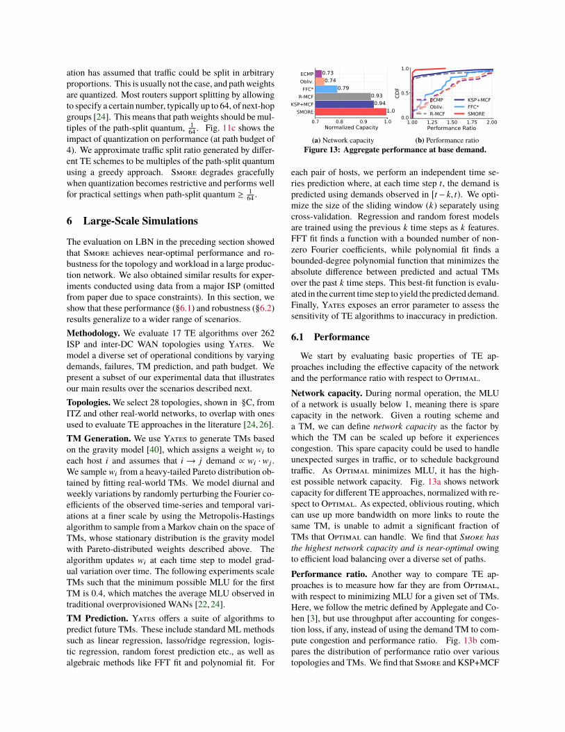
(b) Performance ratioFigure 13: Aggregate performance at base demand.

each pair of hosts, we perform an independent time se-ries prediction where, at each time step t, the demand ispredicted using demands observed in [t − k, t). We opti-mize the size of the sliding window (k) separately usingcross-validation. Regression and random forest modelsare trained using the previous k time steps as k features.FFT fit finds a function with a bounded number of non-zero Fourier coefficients, while polynomial fit finds abounded-degree polynomial function that minimizes theabsolute difference between predicted and actual TMsover the past k time steps. This best-fit function is evalu-ated in the current time step to yield the predicted demand.Finally, Yates exposes an error parameter to assess thesensitivity of TE algorithms to inaccuracy in prediction.

6.1 Performance

We start by evaluating basic properties of TE ap-proaches including the effective capacity of the networkand the performance ratio with respect to Optimal.

Network capacity. During normal operation, the MLUof a network is usually below 1, meaning there is sparecapacity in the network. Given a routing scheme anda TM, we can define network capacity as the factor bywhich the TM can be scaled up before it experiencescongestion. This spare capacity could be used to handleunexpected surges in traffic, or to schedule backgroundtraffic. As Optimal minimizes MLU, it has the high-est possible network capacity. Fig. 13a shows networkcapacity for different TE approaches, normalized with re-spect to Optimal. As expected, oblivious routing, whichcan use up more bandwidth on more links to route thesame TM, is unable to admit a significant fraction ofTMs that Optimal can handle. We find that Smore has

the highest network capacity and is near-optimal owingto efficient load balancing over a diverse set of paths.

Performance ratio. Another way to compare TE ap-proaches is to measure how far they are from Optimal,with respect to minimizing MLU for a given set of TMs.Here, we follow the metric defined by Applegate and Co-hen [3], but use throughput after accounting for conges-tion loss, if any, instead of using the demand TM to com-pute congestion and performance ratio. Fig. 13b com-pares the distribution of performance ratio over varioustopologies and TMs. We find that Smore and KSP+MCF

95.0% 99.0% 99.9% 99.99% 99.999%0.00.20.40.60.81.0

P(T

> x)

(a) base demand, single link failures

95.0% 99.0% 99.9% 99.99% 99.999%0.00.20.40.60.81.0

P(T

> x)

(b) 2× demand, single link failures

95.0% 99.0% 99.9% 99.99% 99.999%0.00.20.40.60.81.0

P(T

> x)

ECMPR-MCFFFC*

KSP+MCFObliv.SMORE

(c) base demand, double link failuresFigure 14: Robustness: Probability of achieving a throughput SLA (x) under different conditions.

0.00 0.05 0.10 0.15Failure Loss

0.6

0.8

1.0

CDF

ECMPObliv.R-MCF

KSP+MCFFFCSMORE

(a) Base demand: failure loss

0.00 0.05 0.10 0.15Congestion Loss

0.6

0.8

1.0

CDF

(b) 2× demand: congestion lossFigure 15: Robustness: CDF of throughput loss

remain optimal in 75-80% of the cases but Smore has

closest to optimal performance ratio (§C.1).

6.2 Robustness

Similar to §5.3, we systematically inject failures inthe network to study the trade-off between performanceand robustness. Fig. 15 shows the distribution of lossin throughput over all possible single link failures. Withbase demands, failures are the main cause of loss. Asdemand scales up, loss due to congestion becomes sig-nificant. Smore performs better in both cases by being

more fault tolerant as well as spreading traffic evenly to

avoid congestion. Although TE approaches like FFC*and R-MCF are designed to be fault tolerant, they do notachieve the best throughput. This is because FFC* re-lies on disjoint paths to be available to reroute traffic; thenumber of such paths is limited in real-world topologies.For instance, GÉANT’s topology has nodes with degree1. These nodes have a single edge-disjoint path to anyother node; the failure of any edge along this path leads toloss of traffic. Using (p,q) link-switch disjoint paths alsodoesn’t improve the robustness much. Moreover, FFC*is not congestion-optimal by design and incurs high lossdue to congestion as demands increase. R-MCF relieson using a large number of paths for fault tolerance andapplying a budget deteriorates its performance [42].

Typically, SLAs refer to availability of a network interms of “nines”. This can also be translated in terms ofthroughput and given a failure characteristic [17, 18, 33],a network operator could be interested in questions suchas “what is the probability that throughput is greater than99.9%?” Fig. 14 compares TE approaches on how likelyare they to achieve different levels of SLA under variousoperational conditions. In addition to the scenario wheresingle link failures can happen with uniform probabil-ity under regular load (Fig. 14a), we perform two moreexperiments where we study robustness under increased

load (Fig. 14b), and concurrent failures (Fig. 14c). Wefind that Smore consistently outperforms other TE ap-proaches. Oblivious TE is robust under both single andconcurrent link failures at base demands, but its resiliencedeteriorates for increased load. Smore benefits from therobust set of paths selected by oblivious routing, andalso load balances efficiently even during increased load.Thus, Smore is highly robust and achieves SLAs with

highest probability under diverse operational conditions.

7 Conclusion

In TE, there is a fundamental trade-off between perfor-mance and robustness. Most systems are designed tooptimize for one or the other, but few manage to achieveboth. This challenge is further exacerbated by operationalrestrictions such as the number of paths, overhead due tochurn, quantized splitting ratio imposed by hardware, etc.

This paper presents Smore, a new approach that navi-gates these trade-offs by combining careful path selectionwith dynamic weight adaptation. As shown through adetailed evaluation on a production backbone network,Smore achieves near-optimal performance in terms ofcongestion and load balancing metrics, is competitivewith shortest-path based approaches in terms of latency,and is also robust, allowing traffic to be re-routed aroundfailures without introducing bottlenecks while respect-ing operational constraints. Our large-scale evaluationshows that these performance and robustness guaranteeshold across a broader class of networks. More generally,our experiences designing and implementing Smore sug-gests lessons that are broadly applicable to TE systemsincluding the importance of capacity-aware and globallyoptimized selection of low-stretch and diverse paths, aswell as the consideration of operational constraints whenbuilding a practical TE system.

Acknowledgments. We would like to thank the anony-mous NSDI reviewers and our shepherd Srikanth Kan-dula for their valuable feedback. This work was partiallysupported by NSF grant CCF-1637532 and ONR grantN00014-15-1-2177. We are grateful to Omar Baldonadoand Sandeep Hebbani for their continued support, andwe thank Bruce Maggs, Ratul Mahajan, Nick McKeown,Jennifer Rexford, Michael Schapira, Amin Vahdat andMinlan Yu for helpful discussions.

References

[1] Historical Abilene Data. http://noc.net.internet2.

edu/i2network/live-network-status/historical-

abilene-data.html.

[2] Altin, A., Fortz, B., and Ümit, H. Oblivious OSPF Routingwith Weight Optimization under Polyhedral Demand Uncertainty.Networks 60, 2 (2012), 132–139.

[3] Applegate, D., and Cohen, E. Making Intra-domain RoutingRobust to Changing and Uncertain Traffic Demands: Understand-ing Fundamental Tradeoffs. In ACM SIGCOMM (2003).

[4] Arora, S., Hazan, E., and Kale, S. The Multiplicative WeightsUpdate Method: a Meta-Algorithm and Applications. Transac-

tions on Computers 8, 1 (2012), 121–164.

[5] Chang, X. Network Simulations with OPNET. In 31st Conference

on Winter Simulation (1999), ACM.

[6] Chang, Y., Rao, S., and Tawarmalani, M. Robust Validationof Network Designs under Uncertain Demands and Failures. InUSENIX NSDI (2017).

[7] Chiesa, M., Kindler, G., and Schapira, M. Traffic Engi-neering with Equal-Cost-MultiPath: An Algorithmic Perspective.IEEE/ACM Transactions on Networking (2016).

[8] Chiesa, M., Rétvári, G., and Schapira, M. Lying Your Way toBetter Traffic Engineering. In ACM CoNEXT (2016).

[9] Elwalid, A., Jin, C., Low, S., and Widjaja, I. MATE: MPLSAdaptive Traffic Engineering. In IEEE INFOCOM (2001).

[10] Fakcharoenphol, J., Rao, S., and Talwar, K. A Tight Boundon Approximating Arbitrary Metrics by Tree Metrics. In 35th

STOC (2003), pp. 448–455.

[11] Building Express Backbone: Facebook’s new long-haul network.http://code.facebook.com/posts/1782709872057497/

building-express-backbone-facebook-s-new-long-

haul-network.

[12] Introducing Open/R - a new modular routing platform.http://code.facebook.com/posts/1142111519143652/

introducing-open-r-a-new-modular-routing-

platform.

[13] Fischer, S., Kammenhuber, N., and Feldmann, A. REPLEX:Dynamic Traffic Engineering Based on Wardrop Routing Policies.In ACM CoNEXT (2006).

[14] Fortz, B., Rexford, J., and Thorup, M. Traffic Engineeringwith Traditional IP Routing Protocols. IEEE Communications

Magazine 40, 10 (Oct. 2002).

[15] Fortz, B., and Thorup, M. Internet Traffic Engineering byOptimizing OSPF Weights. In IEEE INFOCOM (2000), vol. 2.

[16] Garg, N., and Könemann, J. Faster and Simpler Algorithms forMulticommodity Flow and Other Fractional Packing Problems.SICOMP 37, 2 (May 2007), 630–652.

[17] Gill, P., Jain, N., and Nagappan, N. Understanding NetworkFailures in Data Centers: Measurement, Analysis, and Implica-tions. ACM SIGCOMM CCR 41, 4 (2011).

[18] Govindan, R., Minei, I., Kallahalla, M., Koley, B., andVahdat, A. Evolve or Die: High-Availability Design Princi-ples Drawn from Google’s Network Infrastructure. In ACM SIG-

COMM (2016).

[19] Gurobi Optimizer. http://www.gurobi.com.

[20] Hajiaghayi, M., Kleinberg, R., and Leighton, T. Semi-oblivious Routing: Lower Bounds. In SODA (2007), pp. 929–938.

[21] Henderson, T. R., Lacage, M., Riley, G. F., Dowell, C., andKopena, J. Network Simulations with the ns-3 Simulator. SIG-

COMM demonstration 14 (2008).

[22] Hong, C.-Y., Kandula, S., Mahajan, R., Zhang, M., Gill, V.,Nanduri, M., and Wattenhofer, R. Achieving High Utilizationwith Software-Driven WAN. In ACM SIGCOMM (2013).

[23] The Internet Topology Zoo. http://www.topology-zoo.org.

[24] Jain, S., Kumar, A., Mandal, S., Ong, J., Poutievski, L., Singh,A., Venkata, S., Wanderer, J., Zhou, J., Zhu, M., Zolla, J.,Hölzle, U., Stuart, S., and Vahdat, A. B4: Experience with aGlobally Deployed Software Defined WAN. In ACM SIGCOMM

(2013).

[25] Jin, X., Liu, H., Gandhi, R., Kandula, S., Mahajan, R., Rex-ford, J., Wattenhofer, R., and Zhang, M. Dionysus: DynamicScheduling of Network Updates. In ACM SIGCOMM (2014).

[26] Kandula, S., Katabi, D., Davie, B., and Charny, A. Walkingthe Tightrope: Responsive Yet Stable Traffic Engineering. InACM SIGCOMM (2005).

[27] Kelly, F., and Williams, R. Fluid Model for a Network Op-erating under a Fair Bandwidth-Sharing Policy. The Annals of

Applied Probability 14, 3 (2004).

[28] Kumar, A., Jain, S., Naik, U., Raghuraman, A., Kasinadhuni,N., Zermeno, E. C., Gunn, C. S., Ai, J., Carlin, B., Amarandei-Stavila, M., et al. BwE: Flexible, Hierarchical BandwidthAllocation for WAN Distributed Computing. In ACM SIGCOMM

(2015).

[29] Kumar, P., Yu, C., Yuan, Y., Foster, N., Kleinberg, R., andSoulé, R. YATES: Rapid Prototyping for Traffic EngineeringSystems. In ACM SOSR (2018).

[30] Lantz, B., Heller, B., and McKeown, N. A Network in aLaptop: Rapid Prototyping for Software-Defined Networks. InACM HotNets (2010).

[31] Le Roux, J., and Vasseur, J. Path Computation Element (PCE)Communication Protocol (PCEP). https://tools.ietf.org/html/rfc5440, 2009.

[32] Liu, H. H., Kandula, S., Mahajan, R., Zhang, M., and Gel-ernter, D. Traffic Engineering with Forward Fault Correction.In ACM SIGCOMM (2014).

[33] Markopoulou, A., Iannaccone, G., Bhattacharyya, S.,Chuah, C.-N., Ganjali, Y., and Diot, C. Characterization ofFailures in an Operational IP Backbone Network. IEEE/ACM

Transactions on Networking 16, 4 (2008), 749–762.

[34] McCanne, S., and Floyd, S. NS network simulator, 1995.

[35] Mitra, D., and Ramakrishnan, K. A Case Study of Multiser-vice, Multipriority Traffic Engineering Design for Data Networks.In IEEE GLOBECOM (1999), vol. 1.

[36] Cisco NetSim Network Simulator. http://www.boson.com/netsim-cisco-network-simulator.

[37] Panchen, S., Phaal, P., and McKee, N. InMon Corporation’ssFlow: A Method for Monitoring Traffic in Switched and RoutedNetworks. https://tools.ietf.org/html/rfc3176, 2001.

[38] Räcke, H. Minimizing Congestion in General Networks. In 43rd

FOCS (2002), pp. 43–52.

[39] Räcke, H. Optimal Hierarchical Decompositions for CongestionMinimization in Networks. In 40th STOC (2008), pp. 255–264.

[40] Roughan, M., Greenberg, A., Kalmanek, C., Rumsewicz, M.,Yates, J., and Zhang, Y. Experience in Measuring BackboneTraffic Variability: Models, Metrics, Measurements and Meaning.In IMC (2002), ACM, pp. 91–92.

[41] Roy, A., Zeng, H., Bagga, J., Porter, G., and Snoeren, A. C.Inside the Social Network’s (Datacenter) Network. In ACM SIG-

COMM (2015).

[42] Suchara, M., Xu, D., Doverspike, R., Johnson, D., and Rex-ford, J. Network Architecture for Joint Failure Recovery andTraffic Engineering. In SIGMETRICS (2011), pp. 97–108.

[43] Sung, Y.-W. E., Tie, X., Wong, S. H., and Zeng, H. Robotron:Top-down Network Management at Facebook Scale. In ACM

SIGCOMM (2016).

[44] Tardos, E. A Strongly Polynomial Algorithm to Solve Com-binatorial Linear Programs. Operations Research 34, 2 (1986),250–256.

[45] Valiant, L. A Scheme for Fast Parallel Communication. SICOMP

11, 2 (1982), 350–361.

[46] Varga, A., et al. The OMNeT++ Discrete Event SimulationSystem. In European Simulation Multiconference (2001).

[47] Wang, H., Xie, H., Qiu, L., Yang, Y. R., Zhang, Y., and Green-berg, A. COPE: Traffic Engineering in Dynamic Networks. InACM SIGCOMM (2006).

[48] Zhang-Shen, R., and McKeown, N. Designing a Fault-TolerantNetwork Using Valiant Load-Balancing. In IEEE INFOCOM

(Apr. 2008).

A Yates

TE Algorithm #LOC

Shortest Path Routing (SPF) 17

Equal-Cost, Multi-Path (ECMP) 166

Constrained Shortest Path First (CSPF) 287

k-Shortest Paths (KSP) 119

Edge-disjoint k-Shortest Paths (EDKSP) 212

Räcke’s oblivious routing [39] 645

Applegate-Cohen’s oblivious routing [3] 456

Valiant Load Balancing (VLB) [45] 226

Multi-Commodity Flow (MCF) solved as LP [35] 308

MCF solved with Multiplicative Weights (MW) [16] 194

ECMP for paths, MCF for weights (similar to [13]) 474

KSP for paths, MCF for weights (SWAN) [22] 427

EDKSP for paths, MCF for weights 520

Disjoint paths, FFC LP for weights (FFC) [32] 493

Räcke for paths, MCF for weights (Smore) 953

VLB for paths, MCF for weights 534

MCF with failures for paths, MCF for weights (R-MCF) [42] 390

Omniscient MCF (Optimal) 308

Table 3: List of TE algorithms implemented in Yates.

B Illustrations

B.1 Throughput decrease on recovery

One way to recover from failures is to shift traffic onto unaffected paths by re-normalizing the paths weightswhile excluding failed paths. This re-normalization basedrecovery method is fast as it does not need setting up newpaths, and it decreases loss due to failure at the cost ofcongestion. Usually, this increases throughput, but thereare exceptions as illustrated in Fig. 16. Initially, there aretwo A→B paths, but only the direct path (A-B) is beingused and we achieve a total throughput of 3. Failure ofAB link causes all A→B traffic to be dropped and thisreduces the total throughput to 2. Recovery shifts A→B

traffic on to path A-C-B. This causes bottleneck at AC andCB, and the fair share for each flow becomes 0.5. Thisresults in the total throughput further reducing to 1.5.

Another fast way to implement recovery while usingthe unaffected subset of paths is to use a restricted versionof MCF that optimizes for congestion to calculate newweights. But similar to the previous case, throughput candecrease in cases when the minimum possible MLU isgreater than 1.

C Large scale simulations

Topology # nodes(n) # edges (m) Topology # nodes(n) # edges (m)

Abilene 12 15 Airtel 16 26

ATT 25 56 BTNorthAmerica 36 76

CESNET 44 51 CRLNetwork 33 38

CWIX 36 41 Darkstrand 28 31

Digex 31 35 GÉANT 40 61

GRnet 37 42 Google (B4) 12 19

Highwinds 18 31 IBM 18 21

IIJ 37 65 Integra 27 36

Intellifiber 73 95 InternetMCI 19 33

Janet Backbone 32 45 NTT 32 63

PacketExchange 21 27 Palmetto 45 64

Quest 20 31 Sprint 11 18

Tinet 53 89 UUNET 49 84

Xeex 24 34 Xspedius 34 48

Table 4: Topologies used in evaluation.

A B

C

fAB = 1fACB= 0

fAC=

1fC

B=

1

a) Base, tput = 3

A B

C

fAB = 1fACB= 0

fAC=

1fC

B=

1

b) AB fail, tput = 2

A B

C

fAB = 0fACB= 1

fAC=

1fC

B=

1

c) Recovery tput = 1.5

Figure 16: Normalizing path weights to handle failures may

introduce bottlenecks and decrease throughput.

C.1 Performance

Performance ratio. Following Applegate and Cohen,we define performance ratio of a routing scheme r tomeasure how far is it from optimal with respect to mini-mizing congestion for a given TM and topology [3]. Wemodify it slightly to use actual throughput after account-ing for congestion loss, if any, instead of the demand TMto compute congestion. For a TM D, suppose D

r is thethroughput matrix, and dr

uv is the u → v throughput usingr . The maximum congestion for TM D with scheme r is:

maxe∈E

∑u,v dr

uv(e)

cap(e)

where druv(e) denotes the amount of u−v traffic routed

through link e, and cap(e) is the capacity of e. Let OPT

denote the optimal scheme that minimizes maximum linkcongestion. Thus, the performance ratio of r with respectto D is:

perf(r, D) =maxe∈E

∑u,v dr

uv(e)/cap(e)

maxe∈E∑

u,v dOPTuv (e)/cap(e)

In the absence of any loss due to failure, the performance

ratio for any routing scheme is at least 1. This definitioncan be extended for a set of TMs D as:

perf(r,D) =maxD∈D

perf(r, D)

It is the worst performance ratio achieved for any D ∈ D.We find that Smore and SWAN remain optimal in 75-80% of the cases and overall, Smore has closest to optimal

performance ratio.