self-organised critical hot spots of criminal activitynadal/articles/hotspots.pdfself-organised...

Euro. Jnl of Applied Mathematics: page 1 of 29 c© Cambridge University Press 2010

doi:10.1017/S09567925100001851

Self-organised critical hot spotsof criminal activity

H. BERESTYCKI1 and J.-P. NADAL1,2

1Centre d’Analyse et de Mathematique Sociales (CAMS, UMR 8557 CNRS – EHESS), Ecole des Hautes

Etudes en Sciences Sociales, 54 Bd. Raspail, 75270 Paris Cedex 06, France

email: [email protected]

2Laboratoire de Physique Statistique (LPS, UMR 8550 CNRS – ENS – UPMC Univ. Paris 6 – Paris

Diderot Paris 7), Ecole Normale Superieure, 24 rue Lhomond, 75231 Paris Cedex 05, France

email: [email protected]

(Received 7 April 2010; revised 1 June 2010; accepted 1 June 2010)

In this paper1 we introduce a family of models to describe the spatio-temporal dynamics

of criminal activity. It is argued here that with a minimal set of mechanisms corresponding

to elements that are basic in the study of crime, one can observe the formation of hot spots.

By analysing the simplest versions of our model, we exhibit a self-organised critical state

of illegal activities that we propose to call a warm spot or a tepid milieu2 depending on the

context. It is characterised by a positive level of illegal or uncivil activity that maintains itself

without exploding, in contrast with genuine hot spots where localised high level or peaks are

being formed. Within our framework, we further investigate optimal policy issues under the

constraint of limited resources in law enforcement and deterrence. We also introduce exten-

sions of our model that take into account repeated victimisation effects, local and long range

interactions, and briefly discuss some of the resulting effects such as hysteresis phenomena.

1 Introduction

As in other fields, mathematical modelling of criminality has two main scopes. First,

specific models are devised that can be directly confronted with detailed empirical data.

In this spirit, computational criminology is a promising field mainly based on multi-agent

approaches (see e.g. Bernasco 2009; Eck & Liu 2008; Berk 2008). But mathematical models

are also useful in shedding light on mechanisms, and can then be used as quantitative

approaches to help the analysis of more specific models as well as to guide policing

decisions. In this second aspect, stylized facts concerning the level and distribution of

criminal activity are thus both a benchmark and the object of explanations by the model.

Many different types of models have been developed in the criminology literature:

economic and behavioural models (see e.g. Becker 1968; Bourguignon et al. 2003b), some

1 An early and preliminary version of this work has been presented at the workshop Crime Hot

Spots: Behavioral, Computational and Mathematical Models of the Institute for Pure and Applied

Mathematics (IPAM), UCLA, Los Angeles, January 29–February 2, 2007.2 ‘Milieu’: the people, physical and social conditions and events which provide the environment

in which someone acts or lives (Cambridge Dictionary).

2 H. Berestycki and J.-P. Nadal

of them taking into account social interactions (see e.g. Glaeser et al. 1996; Gordon

et al. 2009a), with main tools taken from game theory and models related to the general

framework of discrete choice in socio-economic modelling; epidemic or predator–prey

models making use of ordinary differential equations (ODEs) (see Crane 1991; Campbell

& Ormerod 1998; Nuno et al. 2008); multi-agent simulations (see Eck & Liu 2008; Groff

2007); and reaction–diffusion models describing spatio-temporal patterns of criminal

activity making use of partial diffusion equations (PDEs) (see Short et al. 2008, 2010;

Pitcher 2010) – we refer to Gordon (2010) for a review on mathematical modelling of

criminality. The type of model that we will introduce here makes use of PDEs within an

economic/behavioural approach.

One of the well-documented and outstanding stylized facts in criminology is the

formation, relative stability and persistence of hot spots where high levels of criminal

activities are concentrated. In a relatively recent period, it has become apparent that there

was an overall positive effect on increasing law enforcement in these areas, even if at

the detriment of other neighbourhoods in a city. However, the mechanisms at play in

the formation of hot spots, what determines their persistence, stability issues are still the

object of much investigation with a variety of points of view. Very recent and interesting

studies by Short et al. (2008, 2010) propose a model consisting of a system of reaction-

diffusion equations to describe this phenomenon. We also refer to the bibliography in these

works as well as in Bernasco (2009) for many references on spatial distribution of crime

activities.

The present paper is a contribution to the study of formation, dynamics and other

properties of hot spots of criminal activity. We propose a new model aimed at describing

levels of criminal activity. Since we believe that such approaches are of interest in several

different contexts, we choose to remain vague on the type of criminal activity under

consideration. These can range from uncivil behaviour, traffic offences to petty crimes,

theft and and burglaries. Therefore, in the following, we mostly speak of illegal activity.

Three main issues are addressed in the present paper. The first one is the formation

and stability of hot spots. It is argued here that with a minimal set of mechanisms

corresponding to elements that are basic in the study of crimes, one can observe the

formation of hot spots. Actually, we distinguish here between what we propose to call

warm spot or tepid milieu (depending on their intensity and spatial extension), where a

self-organised critical state of illegal or uncivil activity maintains itself at a positive level

but without exploding, and true hot spot where high level or peaks are being formed.

Then, we propose an approach to investigate optimal policing questions. With neces-

sarily limited law enforcement means and tightening budgets, this question is of high

practical importance. Lessons can be drawn from models, even very theoretical ones, like

the one we discuss here.

Lastly, we set the stage for taking into account other effects: repeated victimisation,

social influence factors or phenomena of diffusion of criminality and deterrence through

social interactions. There are several ways the question of social influence can be addressed

such as long range interaction, collective interaction or local diffusion and interaction. We

briefly describe in the framework of our model a particular trait of crime and punishment

which has been discussed in earlier works, in particular by Ormerod (2005), that of

hysteresis. In few words, this phenomenon bears on the fact that harsher punishment can

Self-organised critical hot spots of criminal activity 3

reduce drastically illegal activity that does not go back to its original high level if the

punishment rate is gradually reduced to its former level.

The main purpose of this paper is to combine all of these complex features into a single

system of a small number of equations. In the present paper we also analyse some of the

simplest situations that arise in this context and argue for their relevance to crime study.

We leave for further studies several mathematical aspects of the more complete system as

well as applications to some more specific questions or further numerical investigations.

2 Dynamics of criminal activity

2.1 The basic model

We consider a spatial domain – a city – where the instantaneous criminal activity u(x, t) at

location x and time t is assumed to depend on an instantaneous willingness (or propensity)

to act, S(x, t). By ‘instantaneous’ we mean an average over some short time scale, but we

do not specify this scale – it could be one hour, or one day, depending on the particular

application considered. The quantity S(x, t) is a spatio-temporal field that may combine

different contributions to the realization of a criminal activity. Taking a coarse-grained

approach, one may consider S(x, t) to represent the typical propensity to commit a crime by

agents at location x. Alternatively, one may consider S(x, t) to represent the propensity of

location x to be the subject of an illegal activity, and this depends on the availability (and

instantaneous willingness to commit a crime) of potential offenders, on the presence of

potential targets at this location, and on the strength of deterrent forces at this location.

This point of view is in line with the Routine Activity Theory developed by Cohen &

Felson (1979) and Clarke & Felson (1993). This general interpretation should be kept in

mind, even though in the following we will mainly make use of the term ‘willingness (or

propensity) to act’. This propensity S is somewhat analogous to the ‘attractiveness’ in the

model of burglary of Short et al. (2008), and to the ‘setting’ variable in Nadal et al. (2010)

(although in the later it is a time independent quantity).

The ‘city’ is defined as an open set Ω in either � or �2. We assume the instantaneous

illegal activity u(x, t) at location x ∈ Ω and time t to be given by a non-linear function of

the local propensity to act. We write

u(x, t) = Λ(S(x, t)). (2.1)

We call Λ the acting-out function. It is assumed to satisfy Λ(S) = 0 for S � 0 and Λ(S) > 0

otherwise, with Λ an increasing function of S > 0 with limit 1 as S goes to infinity. We

define β = Λ′(0+). As examples one may consider

Λ(S) =

{0 if S � 0,

1 − exp(−βS) if S > 0,(2.2)

or

Λ(S) =

⎧⎪⎪⎨⎪⎪⎩0 if S � 0,

βS if 0 < S < 1/β,

1 if S > 1/β.

(2.3)


In the extreme case where one look at a single-agent behaviour, or at the level of a single

illegal act committed in a given neighbourhood:

Λ(S) =

{0 if S � 0,

1 if S > 0,(2.4)

(which corresponds to β → ∞). Actually, we will be mainly interested in the large β

regime, having in mind that acting out is essentially a binary decision – to act or not

to act. Therefore, it corresponds to a threshold type situation, where a sharp transition

occurs at S = 0 which we believe is warranted in analysing criminal activity (a sharp

transition occurs at the very onset of criminal activity).

One of the reasons of the introduction of both a level of criminal activity u and a

propensity to act S is that the former cannot take negative values but the latter can.

Indeed, a point where there is no criminal activity, that is, u = 0 may correspond to a

variety of situations. It is natural to distinguish two cases with no criminal activity but

with one very close to it (S < 0 but close to 0 and the other one where this possibility

is remote (with S very negative). The dynamics of such two places need to be thought of

differently and this is made possible by the introduction of the propensity to act S which

is a characteristic of the location at a given time.

Here, for the sake of simplicity, we assume that there is one globally defined such acting-

out function. In more complex models however, we might envision situations where Λ

also varies with the space variable, for instance, where the territory is divided into patches

and each one of them has its own function Λ. In particular, β could be taken to be a

parameter that varies spatially.

The model we propose for the time evolution of S reads as follows:

∂S

∂t= −S(x, t) + W (x, t) − C(x, t)um(x, t). (2.5)

Let us now explain the meaning of the quantities appearing in this differential equa-

tion (2.5). First, um(x, t) is a moving average of past activity (crime rate). More precisely,

um is defined through the equation:

τu∂um∂t

= u(x, t) − um(x, t), (2.6)

with u(x, t) determined from S through (2.1). Note that (2.5) is written with a time scale

normalised to 1. Thus τu gives the relative time scale for the moving average of the illegal

activity: we assume τu � 1.

Second, C(x, t) is defined to be a local cost of the illegal activity. It represents the

perceived cost of illegal activity resulting from police enforcement and harshness of

punishment. The product C(x, t)um(x, t) thus represents the risk associated with illegal

activity as perceived by potential offenders. The argument, is that a higher past illegal

activity at a given place increases the chances of a ‘cracking down’ by law enforce-

ment authorities. In further versions of this model one may consider a non-linear cost,

by replacing Cum by some non-linear function C(um) involving thresholds, saturations

etc.


Third, W (x, t) is an idiosyncratic willingness (or propensity) to act, which might be

understood as the local expected payoff of a theft, or as an idiosyncratic propensity for

illegal activity at location x and at time t. Note that it is a dishonesty index, corresponding

to the opposite of the honesty index considered in Bourguignon et al. (2003b), Gordon

et al. (2009a) and Nadal et al. (2010). In the simplest setting where W is time independent,

in the absence of illegal activity, (2.5) describes the relaxation of S(x, t) towards W (x).

Next, we specify possible dynamics for the cost term C(x, t) and for the idiosyncratic

propensity for illegal activity W (x, t) (in particular in order to account for repeated

victimisation). We further discuss the introduction of additional terms in order to take

into account social influence and deterrent effects.

2.2 Global and local social influence

We start with the inclusion of a contribution from social interactions in the time evolution

of the instantaneous willingness to act, S . This can be done in two ways: either the influence

is through the observation of the criminal activity, in which case we add a term depending

on a (possibly local) average of the criminal activity; or it comes through a more direct

interaction, resulting in an opinion dynamics, in which case we add a term depending on a

(possibly local) average of the willingness to act. We are thus led to the following system

of equations:

∂S

∂t= −S(x, t) + W (x, t) − C(x, t)um(x, t) +

∫Ω

J(x, x′)um(x′, t) dx′, (2.7)

τu∂um∂t

= Λ(S(x, t)) − um(x, t). (2.8)

The choice of um(x′, t) in the integral term of the first equation above is related to the

observations of repeated offences: Places at which or near which certain crimes have been

committed incur a higher risk of this crime being repeated – as in repeated burglaries.

This effect is discussed below and we include it here in the social influence term. But one

may also consider other factors as relevant for social influence. So more generally, we

consider the system

∂S

∂t= −S(x, t) + W (x, t) − C(x, t)um(x, t) +

∫Ω

J(x, x′)A(x′, t) dx′, (2.9)

τu∂um∂t

= Λ(S(x, t)) − um(x, t). (2.10)

Here, one may choose A(x, t) = um(x, t) as above but other choices are possible:

A(x, t) = S(x, t) or A(x, t) = Sm(x, t), (Sm(x, t) being the time moving average of the

local instantaneous willingness to act, the ‘opinion’ S(x, t)). One may also assume that

agents are aware of their idiosyncratic willingness to act, W , so that it is this ‘intrinsic

opinion’ of the agents which matters, hence A(x, t) = W (x, t).

The kernel J(x, x′) giving the weight of the social influence may have a global part,

which is a part independent of x and x′, and a local part, with a non-zero value only

for close locations. For the later, the simplest natural hypothesis is to assume a diffusive


form. In such case one has the system of equations:

∂S

∂t= −S(x, t) + W (x, t) − C(x, t)um(x, t) + J A(t) + D∇2A(x, t), (2.11)

τu∂um∂t

= Λ(S(x, t)) − um(x, t). (2.12)

For definiteness, one may take A(x, t) ≡ um(x, t) in the above system. To arrive at a

properly posed system, we further require boundary conditions on ∂Ω imposed on S , as

this also reflects on A, since it is a function of um itself a function of S . The most natural

one is the no flux condition:∂S

∂n= 0 on ∂Ω, (2.13)

where n is the outward unit normal vector field on ∂Ω. But other conditions might be

relevant and envisaged as well:

∂um∂n

= g(x, t) on ∂Ω, (2.14)

where g is a given flux of criminal activity, or

∂u

∂n= −ku on ∂Ω (2.15)

for a certain constant k (flux proportional to the instantaneous activity). One may also

consider

u = g(x, t) on ∂Ω (2.16)

that is one assumes an imposed level at the boundary. Such conditions may play an

important role, especially if one isolates a city within its suburban environment.

In this paper, we will only touch on the case of a global social influence, Section 3.5.1.

2.3 Risk aversion, law enforcement and deterrence

2.3.1 Adaptive cost

The simplest way to deal with deterrence here is to assume an adaptive cost: where the

criminal rate is higher than the average, more resources are allocated to this place at the

detriment of elsewhere. We assume a constant total cost, in average over the city the cost

is maintained to a given value C0. We thus consider the simple adaptive rule:

τC∂C

∂t= −C(x, t) + C0 + ηC C0

(um(x, t)

um(t)− 1

). (2.17)

Here and in the following, for any quantity A(x, t) the global (spatial) average is denoted

A(t):

A(t) =

∫Ω

A(x, t)p(x) dx, (2.18)

where p(x) denotes the local population density which is assumed to be constant in time.

In cases where one would have no criminal activity at all, hence um(t) = 0, one would


put 0 in place of the ratio um(t)/um(t). However, such unrealistic situation is clearly of

no interest for the present study, and without loss of generality can be ignored. If the

crime rate remains uniform, um(x, t) = um(t), the cost will relax to the same value C0

everywhere. The time scale τC > 1 depends on the reactivity of the population and on the

law enforcement. With the above updating rule, and provided C(t = 0) = C0, the mean

cost over the population remains constant, C(t) = C0, and if we choose ηC � 1 the cost

C remains non-negative at every location.

An alternative natural choice, equivalent as far as the fixed points of the dynamics are

concerned is to impose at each instant of time a cost equal to a minimal value, plus a

term proportional to the mean crime rate:

C(x, t) = C0(1 − ηC ) + ηC C0um(x, t)

um(t). (2.19)

2.3.2 Deterrence from social interactions

By analogy with our modelling of criminal activity, we introduce a new variable v(x, t),

the instantaneous deterrent activity, with its associated field value D(x, t), the propensity

to contribute to deterrence, and the static reference value D0(x), with

τv∂vm∂t

= v(x, t) − vm(x, t), (2.20)

v(x, t) = ΛD(D(x, t)), (2.21)

where ΛD is a function similar to Λ, and

τD∂D

∂t= −D(x, t) + D0(x) +

∫Ω

L(x, y)D(y, t) dy + R(D, um). (2.22)

The last term characterises the reaction to a non-zero criminal activity. R should be an

increasing function of D and um, if locally there is a large value of u and a large enough

positive D. One may consider R = r(D(x))um(x, t), with r(D) = R0D (R0 > 0) for D � 0

and 0 otherwise. One could also take r(D) � 0 to be a sigmoidal function (going to zero

as D goes to −∞, and to a maximal value R0 for D going to +∞).

To describe the effect of deterrence on the crime rate, we add to the S dynamics,

equation (2.5), a new term proportional to both the (average) criminal and deterrent

activity rates, so that

∂S

∂t= −S(x, t) + W (x, t) − C(x, t)um(x, t) − Kum(x, t)vm(x, t). (2.23)

This is equivalent to have the dynamics (2.5) with an effective cost

Ceff (x, t) = C(x, t) + Kvm(x, t). (2.24)

It will be interesting to compare (2.5) with the adaptive cost, rule (2.17), to the dynamics

(2.23) with C(x, t) = C0(x) – hence comparing two different dynamical rules for the cost

adaptation.


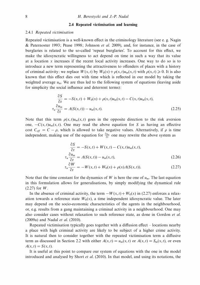
2.4 Repeated victimisation and learning

2.4.1 Repeated victimisation

Repeated victimisation is a well-known effect in the criminology literature (see e. g. Nagin

& Paternoster 1993; Pease 1998; Johnson et al. 2009), and, for instance, in the case of

burglaries is related to the so-called ‘repeat burglaries’. To account for this effect, we

make the idiosyncratic willingness to act depend on time in such a way that its value

at a location x increases if the recent local activity increases. One way to do so is to

introduce a new term representing the attractiveness to offenders of places with a history

of criminal activity: we replace W (x, t) by W0(x)+ρ(x, t)um(x, t) with ρ(x, t) � 0. It is also

known that this effect dies out with time which is reflected in our model by taking the

weighted average um. We are thus led to the following system of equations (leaving aside

for simplicity the social influence and deterrent terms):

∂S

∂t= −S(x, t) + W0(x) + ρ(x, t)um(x, t) − C(x, t)um(x, t),

τu∂um∂t

= Λ(S(x, t)) − um(x, t). (2.25)

Note that this term ρ(x, t)um(x, t) goes in the opposite direction to the risk aversion

one, −C(x, t)um(x, t). One may read the above equation for S as having an effective

cost Ceff = C − ρ, which is allowed to take negative values. Alternatively, if ρ is time

independent, making use of the equation for ∂um∂t

one may rewrite the above system as

∂S

∂t= −S(x, t) + W (x, t) − C(x, t)um(x, t),

τu∂um∂t

= Λ(S(x, t)) − um(x, t), (2.26)

τu∂W

∂t= −W (x, t) + W0(x) + ρ(x)Λ(S(x, t)). (2.27)

Note that the time constant for the dynamics of W is here the one of um. The last equation

in this formulation allows for generalisations, by simply modifying the dynamical rule

(2.27) for W .

In the absence of criminal activity, the term −W (x, t)+W0(x) in (2.27) enforces a relax-

ation towards a reference state W0(x), a time independent idiosyncratic value. The later

may depend on the socio-economic characteristics of the agents in the neighbourhood,

or, e.g. results from a gang maintaining a criminal activity in a neighbourhood. One may

also consider cases without relaxation to such reference state, as done in Gordon et al.

(2009a) and Nadal et al. (2010).

Repeated victimisation typically goes together with a diffusion effect – locations nearby

a place with high criminal activity are likely to be subject of a higher crime activity.

It is natural then to consider together with the repeated victimisation term a diffusive

term as discussed in Section 2.2 with either A(x, t) = um(x, t) or A(x, t) = Sm(x, t), or even

A(x, t) = S(x, t).

It is useful at this point to compare our system of equations with the one in the model

introduced and analysed by Short et al. (2010). In that model, and using its notations, the


attractiveness for buglers at a location x is described by a variable A(x, t) with reference

level B(x), which should be compared to our quantities S(x, t) and W0(x) respectively.

The attractiveness A is increased if a burglary has occurred at this location, relaxes to

the reference level B in the absence of criminal activity, and diffuses to nearby locations.

The burglars’ activity is modelled through a density of burglars who arrive randomly at

any location, diffuse in the neighbourhood until they make a burglary, and then leave the

neighbourhood. In the present model the uncivil or criminal activity is assumed to be a

non-linear function of the local variable S . We do not make explicit assumptions on the

process leading to the criminal act, except through the choice of the acting out function

which characterises the binary nature of the illegal activity, with a threshold phenomenon:

u can be large as soon as S > 0. Note also that here we have an ‘economics’ approach,

where the local attractiveness or willingness to act S is like a surplus: at a fixed point, it

is given by W , a quantity that might be considered as the expected pay-off, plus possible

additional pay-off from social interactions, and minus terms representing a cost.

2.4.2 Learning

In cases where the risk aversion has a positive long-term effect, agents may adapt their

W values, or equivalently the attractivity of places may evolve according to local illegal

activity, in a way which tends to make the local values similar to the ‘norm’, that of the

population average. Then one adds a time dependence in W , with W (x, t = 0) = W0(x) and

τw∂W

∂t= −W (x, t) + W0(x) − ηw(Gm(x, t) − Gm(t)) (2.28)

with Gm(x) is the moving average of C(x, t)u(x, t), and Gm is the average of Gm over the

city. This adaptation occurs on a time scale much larger than the one of S , hence τw � 1.

This time scale might be of the same order as τu, the one controlling the moving average

of u, since both correspond to time scales affecting agents perception of time. The above

learning rule corresponds to a long-term deterrent effect of punishment: for large mean

suffered costs the willingness to act decreases.

The choice of Cum as the source of W modification can be discussed. Not that this

term has the correct dimension (the one of W ).

2.5 Links with neural models of decision making

The (family of) model(s) that we have introduced here is somewhat reminiscent of the

‘Integrate and Fire’ models in theoretical neuroscience (see e.g. Chow et al. 2004; Brunel &

van Rossum 2007). In this context, (2.5) gives the dynamics of the post-synaptic potential

S of neuron indexed by x, with firing rate um, and, if Λ is the binary function, u is the

spiking activity (spike/no spike). Otherwise, Λ is the transfer function and u the spiking

rate. The cost term corresponds to an autapse, a synaptic connection of the neuron onto

itself. Here this connection is inhibitory. The term W corresponds to the external input

minus the activation threshold. An apparent difference with a neural model is that here

S can be negative, whereas the post-synaptic potential is a positive quantity. However,

one can note that, if W and C are bounded from below, one can subtract a constant to


S and work with a positive variable. The social interaction term gives the inputs from

other neurons, with excitatory synaptic weights J(x, x′) from cell x′ to cell x. The model

with social deterrence corresponds to a classical scheme of an assembly of cells composed

of two sub-populations, one of excitatory neurons, described by S and u, and one of

inhibitory neurons described by the variables D and v. In the present model, however, the

interactions between these two populations are different from what one usually considers

in neuroscience, although these interactions do have a biological correspondence: a term

like −Kumvm is analogous to having an heterosynaptic interaction – the synaptic input

from a cell (here an inhibitory one) onto another one (here an excitatory cell) is gated by

the activity of another cell (here of the target cell itself).

The dynamics considered here has still another important difference with the one of

neural systems: after a spike, the membrane potential goes back to a resting state, and

there is a ‘refractory period’, a short time during which no spike can be emitted. Here, in

the case of a sharp activation function (Λ = 0 or 1), the reset would be equivalent to, say,

reset S to W whenever u = 1.

In any case, the dynamics of S may be thought of as reflecting the integration dynamics

at the neural level – that of a single neuron or of a network. Such neural dynamics is

considered to be at the basis of any decision by the evidence accumulation in favour or

against a particular alternative, an action being taken when this accumulation reaches

some threshold.

Lastly, we have introduced the possibility of learning or adaptation, for the ‘autapse’ C

and for the idiosyncratic term W . The chosen learning rules depend on the correlations

between punishment and activity, which is reminiscent of (but not identical to) ‘reinforce-

ment learning rules’ considered as the basis of behavioural learning at the neural level.

In the neural context, what matters is the actual punishment (or reward). Here what we

consider has ambiguously the meaning of either the expected punishment or the mean

punishment incurred so far. It would indeed be interesting to explicitly take into account

whether the agents have been punished or not. Particular dynamics based on the actual

effect of punishment are considered in Gordon et al. (2009a) and Nadal et al. (2010).

3 Analysis

This section is devoted to a mathematical analysis of the large time limit of our dynamical

system. The results are illustrated by numerical simulations.

3.1 Time independent W and C

3.1.1 Single location dynamics

Consider first W and C constant in time: W (x, t) = W (x) and C(x, t) = C(x). We have

then a set of (spatially) uncoupled equations, so that, in this section, we can drop the

index x for the moment, first studying the two coupled equations for given values of the

scalars C > 0 and W :

dS(t)

dt= −S(t) + W − Cum(t), (3.1)

τudum(t)

dt= Λ(S(t)) − um(t). (3.2)


We assume that the acting out function Λ satisfies Λ(S) = 0 for S � 0 and Λ(S) > 0

otherwise, with Λ a C1 increasing function on [0,+∞], satisfying Λ(0+) = 0 and having

limit 1 as S goes to infinity. We define β = Λ′(0+). We will be particularly interested here

on the large β limit.

The fixed points of the dynamics (3.2) are given by

S∗ = W − CΛ(S∗), (3.3)

u∗m = Λ(S∗). (3.4)

Given the properties of the function Λ one easily sees that for each given values of {W,C}there is a unique solution. For W < 0,

S∗ = W, (3.5)

u∗m = 0. (3.6)

For W > 0, S∗ > 0 is the unique intersection of the graphs y = S and y = W − CΛ(S)

for S � 0. Clearly, the larger W > 0, the larger S∗ and the larger the illegal activity u∗m.

The stability is determined by the linearisation of (3.2) near the fixed point. For W < 0,

one gets the matrix(−1 −C

0 − 1τu

)having eigenvalues −1 and −1/τu.

For W > 0, one gets the 2 × 2 matrix⎛⎜⎝ −1 −C

β∗

τu− 1

τu

⎞⎟⎠ (3.7)

with β∗ ≡ Λ′(S∗) > 0. The eigenvalues are given by

For β∗C �(τu − 1)2

4τu, λ± = −τu + 1

2τu± 1

2τu[(τu − 1)2 − 4τuβ

∗C]1/2. (3.8)

For β∗C >(τu − 1)2

4τu, λ± = −τu + 1

2τu± i

2τu[4τuβ

∗C − (τu − 1)2]1/2. (3.9)

The real part of the eigenvalues are always negative, so that the fixed point is always stable.

In the case (3.9), convergence towards the fixed point occurs with damped oscillations.

This is the case for β∗ large enough, that is for W smaller than C if the function Λ has a

steep slope at S > 0, as illustrated in Figure 1.

3.1.2 Large β limit

We consider a family of acting out functions indexed by the slope β at S = 0+, as (2.2)

or (2.3). More precisely, we assume that, when β → ∞, the acting out function Λ = λβconverges to the step acting out function defined in (2.4). For βC large, when 0 < W < C ,

at first order in 1/βC the fixed point is given by

S∗ =W

βC, (3.10)

u∗m =

W

C

(1 − 1

βC

). (3.11)


−0.2 −0.1 0 0.1 0.2 0.3 0.40

0.2

0.4

0.6

0.8

1(a) (b)

(c) (d) (e)

S

Λ(S)

β = 25

−0.2 0 0.2 0.4 0.6 0.8

−0.2

0

0.2

0.4

0.6

0.8

1

1.2

1.4

1.6

S

W = 0.5

W = 1.5β = 25

C = 1

W − C Λ(S)

0 100 200 300 400 500−0.2

0

0.2

0.4

0.6

0.8

1

1.2

1.4

1.6

time

S(t)

W = 0.5

W = 1.5

0 100 200 300 400 5000

0.2

0.4

0.6

0.8

1

time

u(t)

0 100 200 300 400 500 6000

0.2

0.4

0.6

0.8

1

time

um

(t)

β = 25C = 1

W = 1.5

W = 0.5

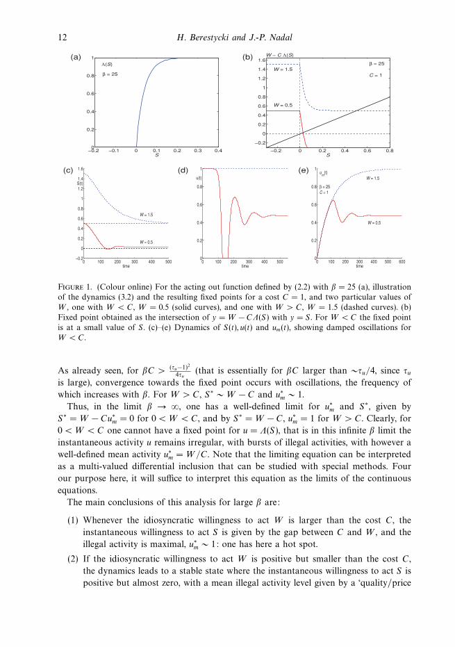
Figure 1. (Colour online) For the acting out function defined by (2.2) with β = 25 (a), illustration

of the dynamics (3.2) and the resulting fixed points for a cost C = 1, and two particular values of

W , one with W < C , W = 0.5 (solid curves), and one with W > C , W = 1.5 (dashed curves). (b)

Fixed point obtained as the intersection of y = W − CΛ(S ) with y = S . For W < C the fixed point

is at a small value of S . (c)–(e) Dynamics of S (t), u(t) and um(t), showing damped oscillations for

W < C .

As already seen, for βC > (τu−1)2

4τu(that is essentially for βC larger than ∼τu/4, since τu

is large), convergence towards the fixed point occurs with oscillations, the frequency of

which increases with β. For W > C , S∗ ∼ W − C and u∗m ∼ 1.

Thus, in the limit β → ∞, one has a well-defined limit for u∗m and S∗, given by

S∗ = W − Cu∗m = 0 for 0 < W < C , and by S∗ = W − C , u∗

m = 1 for W > C . Clearly, for

0 < W < C one cannot have a fixed point for u = Λ(S), that is in this infinite β limit the

instantaneous activity u remains irregular, with bursts of illegal activities, with however a

well-defined mean activity u∗m = W/C . Note that the limiting equation can be interpreted

as a multi-valued differential inclusion that can be studied with special methods. Four

our purpose here, it will suffice to interpret this equation as the limits of the continuous

equations.

The main conclusions of this analysis for large β are:

(1) Whenever the idiosyncratic willingness to act W is larger than the cost C , the

instantaneous willingness to act S is given by the gap between C and W , and the

illegal activity is maximal, u∗m ∼ 1: one has here a hot spot.

(2) If the idiosyncratic willingness to act W is positive but smaller than the cost C ,

the dynamics leads to a stable state where the instantaneous willingness to act S is

positive but almost zero, with a mean illegal activity level given by a ‘quality/price


0 0.2 0.4 0.6 0.8 1−0.5

0

0.5

1(a) (b)

x

u*

S*

W

C=C0

0 0.5 1 1.5 2 2.5 30

0.1

0.2

0.3

0.4

0.5

0.6

0.7

0.8

0.9

1

W /C

um*

(W > 0)

Figure 2. (Colour online) (a) Fixed points for the acting out function defined by (2.2) with β = 50,

with a constant cost C = 0.2 (solid horizontal line), for a particular spatial pattern of idiosyncratic

values W (x) (dot-dashed curve), with a uniform population density on [0, 1]. Dot curve: u∗m; solid

curve: S ∗. (b) For this simulation, plot of the activity u∗m as function of W/C . For W/C of order

1 there is a crossover from the linear behaviour u∗m = W/C to the saturation at maximal activity,

u∗m = 1.

ratio’, W/C . This state can be considered as a self-organised critical state (since

S = 0 is the critical value at which there would be no illegal activity), where the

illegal activity is positive but remains moderate (on the concept of self-organised

criticality, see Bak 1997). We propose to call such state a warm spot. In some cases,

such as the case of uncivil behaviour, one may assume that W is positive but small

almost everywhere. Then essentially all the space is in this self-organised critical

sate (with possibly some hot spots, as well as some quiet spots where W < 0): we

propose to call this a tepid milieu.

Figure 2 illustrate the fixed points obtained for a particular spatial pattern of idio-

syncratic values W (x) having two underlying hot spots (positive values of W in two

neighbourhoods) for a (moderately) large value of β.

3.2 Optimal control

Under the hypotheses considered in the previous section, it is clear that one would like to

have the cost C larger than the idiosyncratic willingness to act W . Still ignoring possible

social interaction effects, let us address the issue of optimal control under the constraint

of limited resources.

Assume that on the spatial domain Ω under consideration, there is at each location

x ∈ Ω a particular time independent value W (x) of the idiosyncratic willingness to act,

and continue to assume that the acting out function Λ is independent of the location and

characterised by a large β value. Now we study the (realistic) scenario when there is a

global limit imposed on available resources to enforce a cost on illegal activity. We want to

compute the cost function C(x) such that the mean illegal activity is minimised, under the

constraint that the total cost – hence the mean cost averaged over all locations – is given.

We assume the criminal activities given by the fixed point equations, defined by (3.6)

at locations x where W (x) < 0, and (3.11) where W (x) � 0. Since the crime rate um


−0.25 0 0.5 0.75 10

0.002

0.004

0.006

0.008

0.01

0.012

0.014

0.016

0.018

0.02

W

P(W)

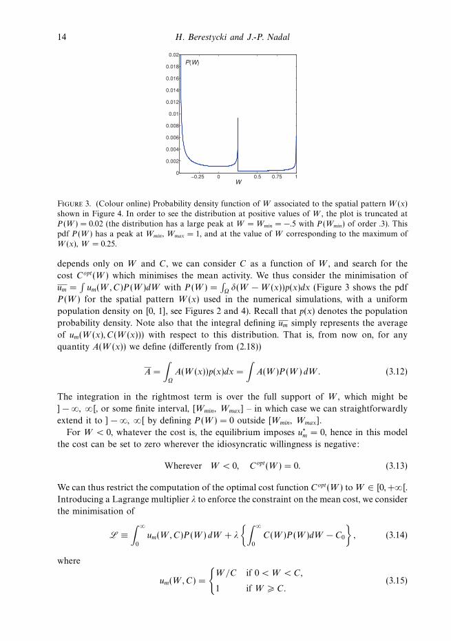
Figure 3. (Colour online) Probability density function of W associated to the spatial pattern W (x)

shown in Figure 4. In order to see the distribution at positive values of W , the plot is truncated at

P (W ) = 0.02 (the distribution has a large peak at W = Wmin = −.5 with P (Wmin) of order .3). This

pdf P (W ) has a peak at Wmin, Wmax = 1, and at the value of W corresponding to the maximum of

W (x), W = 0.25.

depends only on W and C , we can consider C as a function of W , and search for the

cost Copt(W ) which minimises the mean activity. We thus consider the minimisation of

um =∫um(W,C)P (W )dW with P (W ) =

∫Ωδ(W − W (x))p(x)dx (Figure 3 shows the pdf

P (W ) for the spatial pattern W (x) used in the numerical simulations, with a uniform

population density on [0, 1], see Figures 2 and 4). Recall that p(x) denotes the population

probability density. Note also that the integral defining um simply represents the average

of um(W (x), C(W (x))) with respect to this distribution. That is, from now on, for any

quantity A(W (x)) we define (differently from (2.18))

A =

∫Ω

A(W (x))p(x)dx =

∫A(W )P (W ) dW. (3.12)

The integration in the rightmost term is over the full support of W , which might be

] − ∞, ∞[, or some finite interval, [Wmin, Wmax] – in which case we can straightforwardly

extend it to ] − ∞, ∞[ by defining P (W ) = 0 outside [Wmin, Wmax].

For W < 0, whatever the cost is, the equilibrium imposes u∗m = 0, hence in this model

the cost can be set to zero wherever the idiosyncratic willingness is negative:

Wherever W < 0, Copt(W ) = 0. (3.13)

We can thus restrict the computation of the optimal cost function Copt(W ) to W ∈ [0,+∞[.

Introducing a Lagrange multiplier λ to enforce the constraint on the mean cost, we consider

the minimisation of

L ≡∫ ∞

0

um(W,C)P (W ) dW + λ

{∫ ∞

0

C(W )P (W )dW − C0

}, (3.14)

where

um(W,C) =

{W/C if 0 < W < C,

1 if W � C.(3.15)


0 0.2 0.4 0.6 0.8 1−0.5

0

0.5

1(a) (b)

(c) (d) (e)

x

W(x)

0 0.2 0.4 0.6 0.8 1

0

0.5

1

1.5

x

u*C*S*W

−0.2 0 0.2 0.4 0.6 0.80

0.2

0.4

0.6

0.8

1

1.2

1.4

1.6

W

C*

C0

0 0.2 0.4 0.6 0.80

0.5

1

1.5

um*

C*

−0.2 −0.1 0 0.1 0.20

0.2

0.4

0.6

0.8

1

S*

um*

W−S*/C*

Λ(S*)

Figure 4. (Colour online) Case of an adaptive cost (as defined Section 2.3.1 and analysed Section

3.3). For the acting out function defined by (2.2) with β = 50, illustration of the fixed points of the

dynamics (3.26) for a pattern of idiosyncratic values W (x) shown on (a)–(b). Same W pattern and

parameters as for Figure 2, with here a mean cost value C0 equal to the value of the constant cost

in Figure 2, C0 = 0.2.

Assume that one can achieve a solution with C > W everywhere. For W > 0, setting to

zero the functional derivative of L with respect to C gives

−W

C2+ λ = 0 (3.16)

which leads to C proportional to the squareroot of W , and with the constraint on the

average of C one gets

Copt(W ) = C0 W1/2/W 1/2, (3.17)

where we recall that the bar denotes the average over the space, or equivalently over the

W distribution, which is here W 1/2 =∫ ∞

0 W 1/2P (W ) dW . For this optimal cost function,

the mean crime rate is

umopt =

(W 1/2 )2

C0(3.18)

and at a location with idiosyncratic willingness to act W � 0, the mean crime rate is

uoptm =W 1/2

C0W 1/2. (3.19)

It is worth noticing that, at this optimal solution, the crime rate is not reduced to the

same value everywhere. Compared to the solution that would be obtained with a same


value C0 everywhere (that is um = um(W,C0)), one has a strong reduction of the criminal

activity where W > C0, and where W < C0 one has uoptm /um(W,C0) = W 1/2/W 1/2. Hence

the price to pay to reach the minimal mean crime rate is to accept a larger criminal

activity at locations where W 1/2 is smaller than the average value of W 1/2.

The above solution (3.17) is valid if one has indeed W < Copt(W ) for all values of W

with P (W ) > 0, that is, if Wmax is the largest value taken by W (x) for x ∈ Ω, if

W 1/2max W 1/2 < C0. (3.20)

The equality C0 = W1/2max W 1/2 gives the minimal global amount of resource for which

no location in Ω will have the maximal crime rate. In the unfortunate case where

W1/2max W 1/2 > C0, the optimal cost is proportional to the square root of W up to a

threshold value Wc at which Copt(Wc) = Wc, and then the cost is kept at this value

maximal value Cmax = Wc for all W > Wc:

Copt(W ) =

⎧⎪⎪⎨⎪⎪⎩0 if W � 0,

W1/2c W 1/2 if 0 < W � Wc,

Cmax = Wc if W > Wc.

(3.21)

The threshold value Wc < Wmax is given by the constraint on the mean cost, which can

be written here

C0 = W 1/2c

(W 1/2 −

∫ Wmax

Wc

(W 1/2 − W 1/2c )P (W ) dW

). (3.22)

For the optimal cost function, one gets that the mean crime rate takes a very simple

expression,

umopt =

C0

Cmax

, (3.23)

where we recall that Cmax = Wc is solution of (3.22). One can check that this expression

gives back (3.18) at C0 = W1/2max W 1/2. For illustrative purpose, consider the case of

a uniform distribution of W on [0,Wmax] (and no negative values at all). One gets

W 1/2 = 2Wmax/3. The places with um = 1, can be avoided with a mean cost at least

equal to two third of the maximal value of W . Otherwise, for Wmax > 3C0/2, Wc =32Wmax(1 − [1 − 4C0

3Wmax]1/2).

Beside the constraint on the mean cost, there may exist a maximal value C1 of the cost

resulting from the maximal resources that can be provided locally at a given location. In

that case, the solution (3.21) cannot be realized if C1 < Wc, and the least worst choice is

to have the cost given by the expression (3.21) with Wc replaced by C1.

The optimal policy for the choice of the cost depends on the knowledge of the

idiosyncratic willingness to act W , which is not an observable quantity. In the next

section, we will see that the simple cost adaptation rules (2.17) and (2.19) proposed in

Section 2.3.1 allow one to enforce the optimal policy from the observation of the illegal

activity alone.


3.3 Cost adaptation

Let us now add to the dynamics the cost adaptation rule (2.17), still keeping W (x) time

independent. Since the cost C(x, t) has a dynamics which depends on the mean crime rate

averaged over all locations, um(t), the dynamics at the different locations are coupled, but

coupled only through this collective variable:

∂S(x, t)

∂t= −S(x, t) + W (x) − C(x, t) um(x, t), (3.24)

τu∂um(x, t)

∂t= Λ(S(x, t)) − um(x, t), (3.25)

τC∂C(x, t)

∂t= −C(x, t) + C0 + ηC C0

(um(x, t)

um(t)− 1

), (3.26)

with um(t) =∫Ωum(x, t)p(x) dx.

A a fixed point, the quantities of interest depend on the location x only through W (x).

Anticipating the uniqueness of the solution, we can consider all quantities as functions of

W (instead of space x), and write the fixed point equations as

S∗(W ) = W − C∗(W ) u∗m(W ), (3.27)

u∗m(W ) = Λ(S∗(W )), (3.28)

C∗(W ) = (1 − ηC )C0 + ηC C0u∗m(W )

u∗m

, (3.29)

with u∗m(t) =

∫u∗m(W, t)P (W ) dW . For locations where W < 0, it is obvious that the

solution, unique and stable, is given by S∗(W ) = W , u∗m = 0 and C∗ = (1 − ηC )C0, the

smallest possible value that can be taken by the cost C∗. We can now restrict the analysis

to the set of locations with W > 0 and, again, we consider the limit of large β. In this

limit, for W > 0 we can rewrite the fixed point equations (3.27) and (3.28) as

S∗(W ) =

{0+ if W � C∗(W ),

W − C∗(W ) if W > C∗(W ),(3.30)

u∗m =

{W/C∗(W ) if W � C∗(W ),

1 if W > C∗(W ).(3.31)

Let us consider the particular case ηC = 1. First, assume that the condition W � C∗(W ) is

always true. Then one readily gets that C∗ is proportional to the square root of W , which

gives exactly the expression (3.17) of the cost. As already seen in the previous section, this

optimal situation will be reached provided the condition (3.20) is met. Otherwise, there

is a maximal cost C∗max = C0/u∗

m reached for every value of W larger than some critical

value: again one gets exactly the optimal cost function, the one given by the expression

(3.21) for cases where (3.20) is not valid.

For ηC < 1, one gets a sub-optimal solution, with

C∗(W ) =1 − ηC

2C0 +

[ηC

W

u∗m

+(1 − ηC )2

4C2

0

]1/2

, (3.32)


and the global parameter u∗m is determined by the normalisation condition u∗

m = W/C∗(W ).

In our model, there is no criminal activity at all for W < 0, which might be considered

as a too strong hypothesis. A plausible variant would be to have an acting out function

taking non-zero but very small values for W < 0, or, one may add some noise in the

dynamics of S , which would have the same qualitative effect. In such cases, a small but

non-zero cost would be necessary as well, hence one would have to take a value of ηCsmaller than one. We leave to future work a more detailed analysis of such case.

The main conclusion of this section is thus that a simple adaptation rule, which makes

the cost proportional to the local crime rate, is sufficient to enforce the optimal policy

without the knowledge of the unobservable variables which characterise the propensity

to commit crime. In order to get rid of the hottest spots, the places out of control where

the crime rate is maximal, one may have to increase the global available resource C0.

Within the present scheme, the minimal necessary global resource can be reached from

a progressive increase of C0 until the point where there is no more any domain with

um = 1.

3.4 Social deterrence

Let us go back to the case C constant and homogeneous, C(x, t) = C0(x) = C0, and

study the specific effect of deterrence as described by (2.20)–(2.23). Without any non-local

interaction, the equations for a location with particular values D0 > 0 and W0 are then

dS(t)

dt= −S(t) + W0 − (C0 + Kvm(t)) um(t), (3.33)

τudum(t)

dt= Λ(S(t)) − um(t), (3.34)

τvdvm(t)

dt= ΛD(D(t)) − vm(t), (3.35)

τDdD(t)

dt= −D(t) + D0 + R0D(t) um(t), (3.36)

where R = R0D(t) um with 0 < R0 < 1. Equation (3.33) can be rewritten as

dS(t)

dt= −S(t) + W0 − Ceff (t)um(t), (3.37)

τvdCeff (t)

dt= −Ceff (t) + C0 + K ΛD(D(t)), (3.38)

with Ceff (t) ≡ C0 + Kvm(t). These equations have to be compared to the ones with cost

adaptation but no deterrence, (3.26). Here the dynamics of the effective cost is more

complex, but is purely local. We will not give a full analysis of this system, but focuses

on the fixed points equations, which for R0 < 1 can be written as

S∗ = W0 − C∗eff u

∗m, (3.39)

u∗m = Λ(S∗), (3.40)


0 0.2 0.4 0.6 0.8 1

−0.4

−0.2

0

0.2

0.4

0.6

0.8

1

x

W

Ceff*

S*

u*

D*

Figure 5. (Colour online) Case of social deterrence (as defined Section 2.3.2 and analysed Sec-

tion 3.4), with a constant cost C = C0. Plot of W (x) (dash-dot curve), and of the fixed point

values of the effective cost Ceff (upper dashed curve), D (lower dashed curve) and S (solid curve).

Parameters: C0 = 0.2, D0 = 0.02, R0 = 0.8, K = 1.; acting out and deterrence functions given by

(2.2) with, respectively, β = 50 and βD = 25; same values of C0, β and same pattern W (x) as in

Figures 2 and 4.

C∗eff = C0 + K ΛD(D∗), (3.41)

D∗ =D0

1 − R0u∗m

. (3.42)

For W0 < 0, one still has the obvious solution S∗ = W0, u∗m = 0, v∗

m = ΛD(D0). For

W0 > 0, as before, we focus on the large β limit. The maximal possible value of C∗eff is

Cmaxeff = C0 +KΛD(D0/(1−R0)). From the analysis done before we know that if W0 > Cmax

eff

one has the solution u∗m ∼ 1, S∗ = W0 − Cmax

eff , D∗ = D0/(1 − R0).

Otherwise, that is if W0 < Cmaxeff , S∗ is not too large, Λ(S∗) ∼ βS∗, and one gets

S∗ = W0/(1 + βC∗eff ), with C∗

eff at least equal to C0. Hence S∗ goes to zero as β goes to ∞,

and u∗m = W0/C

∗eff , with C∗

eff obtained as the solution of

C∗eff = C0 + K ΛD

(D0

1 − R0W0/C∗eff

). (3.43)

This equation has a unique solution for W0 < Cmaxeff = C0 + KΛD(D0/(1 − R0)) since ΛD

is a strictly increasing function of its (positive) argument.

The results are thus qualitatively similar to the case with an adaptive cost (see Figure 5),

except that here the deterrent resources are purely local, hence less efficient. In the

preceding case, available resources are concentrated on locations where a higher deterrent

or law enforcement is needed, and the highest possible value of C that can be found in

the stationary regime is C0 + ηCC0(1 − um)/um, which is at most C0/um. Here the maximal

deterrent effect is given by the maximal possible value of the effective cost C + Kumvmwhich is the constant C0 + K . In the cost adaptation case one has a multiplicative effect,

whereas here one has an additive effect. There is thus a self-adaptation mechanism in

the first case which is strongly limited in the present case. Limiting the criminal activity

requires to tune the parameter K in order to have everywhere C(x) > W (x). Such

condition is much more likely to be met in the first case, thanks to the recruitment of


resources from locations where there is no need for a strong cost, and to the multiplicative

effect on the largest cost values.

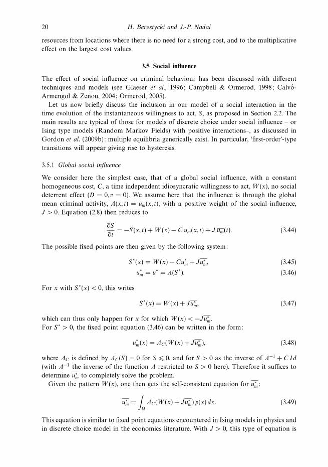
3.5 Social influence

The effect of social influence on criminal behaviour has been discussed with different

techniques and models (see Glaeser et al., 1996; Campbell & Ormerod, 1998; Calvo-

Armengol & Zenou, 2004; Ormerod, 2005).

Let us now briefly discuss the inclusion in our model of a social interaction in the

time evolution of the instantaneous willingness to act, S , as proposed in Section 2.2. The

main results are typical of those for models of discrete choice under social influence – or

Ising type models (Random Markov Fields) with positive interactions–, as discussed in

Gordon et al. (2009b): multiple equilibria generically exist. In particular, ‘first-order’-type

transitions will appear giving rise to hysteresis.

3.5.1 Global social influence

We consider here the simplest case, that of a global social influence, with a constant

homogeneous cost, C , a time independent idiosyncratic willingness to act, W (x), no social

deterrent effect (D = 0, v = 0). We assume here that the influence is through the global

mean criminal activity, A(x, t) = um(x, t), with a positive weight of the social influence,

J > 0. Equation (2.8) then reduces to

∂S

∂t= −S(x, t) + W (x) − C um(x, t) + J um(t). (3.44)

The possible fixed points are then given by the following system:

S∗(x) = W (x) − Cu∗m + Ju∗

m, (3.45)

u∗m = u∗ = Λ(S∗). (3.46)

For x with S∗(x) < 0, this writes

S∗(x) = W (x) + Ju∗m, (3.47)

which can thus only happen for x for which W (x) < −Ju∗m.

For S∗ > 0, the fixed point equation (3.46) can be written in the form:

u∗m(x) = ΛC(W (x) + Ju∗

m), (3.48)

where ΛC is defined by ΛC(S) = 0 for S � 0, and for S > 0 as the inverse of Λ−1 + C Id

(with Λ−1 the inverse of the function Λ restricted to S > 0 here). Therefore it suffices to

determine u∗m to completely solve the problem.

Given the pattern W (x), one then gets the self-consistent equation for u∗m:

u∗m =

∫Ω

ΛC(W (x) + Ju∗m) p(x) dx. (3.49)

This equation is similar to fixed point equations encountered in Ising models in physics and

in discrete choice model in the economics literature. With J > 0, this type of equation is


0 1 2 4 6 8 10

−6

−5

−4

−3

−2

−1

0

1

β(J − C)

β W

[β(J − C)]c=1

Figure 6. (Colour online) Global social influence: Domain (dashed area) of multiple solutions in

the parameter space, in the case of a homogeneous W value, and with the acting out function (2.2).

known to have generically multiple solutions – that is, there is a wide range of parameters

for which there exists several solutions. The analysis of the solutions of this equation is

analogous to the one done in Nadal et al. (2006), Gordon et al. (2009b). It is sketched in

the Appendix.

For the simplest case of a homogeneous distribution of W values (W = W everywhere),

in which case the fixed point equation simplifies to

u∗m = Λ(W + (J − C)u∗

m), (3.50)

Figure 6 shows the phase diagram: in parameters space, the domain where the fixed point

equation (3.49) has two solutions, one with u∗m = 0 (which would be the solution in the

absence of social influence), and one with u∗m > 0 (see the Appendix for details).

We leave to future work a more detailed analysis of the fixed point solutions and their

stability in more general cases.

3.5.2 Hysteresis

As noted by Gordon et al. (2009b), the domain of multiple solutions lies in the part of the

parameters space corresponding to populations which, in average, are not willing to act

(that is at negative values of W here). This means that hot spots of criminal activity may

be caused purely by collective effects at locations where, with the same socio-economic

characteristics, one could equally observe a ‘quiet’ spot. One can thus expect that such

hot spots can be reduced, thanks to, or despite, the hysteresis effect associated to these

multiple equilibria. This is the object of the discussion below.

There is a considerable literature on hysteresis in choice models and related models

like Ising spin systems. We refer in particular to Sethna (2009) for various applications

in physics, to Nadal et al. (2006) for choice models in a socio-economics context, and to

Ormerod (2005) for a very interesting discussion of the implications of hysteresis in the

context of crime modelling. We reconsider the later within our framework.

Let us consider the simple case of a homogeneous distribution of W (for which the

phase diagram is shown on Figure 6). Figure 7 illustrate the solutions um∗ as function of


0 1 2 3 4 5 60

0.2

0.4

0.6

0.8

1

β(J − C)

um*

β W = −1/2

−2 −1 0 10

0.2

0.4

0.6

0.8

1

β W

um*

β (J − C) = 3

Figure 7. (Colour online) Fixed point solutions um∗ under a global social influence with a homo-

geneous distribution of W values, and the acting out function (2.2). (a) Solutions versus β(J − C)

keeping βW = −0.5 fixed. The solution um∗ = 0 always exists. (b) Solutions versus βW keeping

β(J − C) fixed. The solution um∗ = 0 only exists for W < 0.

the reduced parameter J ≡ β(J −C) at a given value of W ≡ βW < 0, and as function of

βW at a given value of J > Jc. In the first case, at small J there only exists the solution

um∗ = 0. At a critical value which depends on βW , Jc(βW ), one enters the domain of

multiple solutions: a solution with a high level of criminality appears abruptly. If the

dynamics starts at a value J < Jc(βW ), the systems converge to the unique fixed point

um∗ = 0. If J is increased, the dynamical system will stay at this fixed point which is

always stable. Only a strong external perturbation may make the system jump to the high

criminal state in the range J > Jc(βW ). Once in this state, the system will remain on

the upper branch of solutions if J is decreased – which will be the case if the cost C is

increased –, until the critical point where this solution disappears. A that point the system

jumps back to the quiet state with no criminal activity. Then the cost C can be decreased

(hence J increases again), the system remaining in this quiet state.

For this particular simple model, the upper branch um∗ > 0 exists for all J > Jc(W ).

This needs not be the case in general (see e.g. Gordon et al. 2009b), that is one expects the

upper boundary of the domain of multiple solutions in the plane (J,W ) to be generically

given by a critical value of W which is a decreasing function of J . In the present simple

case of a homogeneous W , the situation at a given value of W will look more similar to

the behaviour of the solutions at a constant J > Jc when one increases W from a low

negative value to a positive value, as illustrated on the right panel of Figure 7. That is,

there will be an upper critical value of J for which the quiet state, um∗ = 0, disappears,

leaving as a unique solution a fixed point with um∗ > 0.

3.6 Repeated victimisation

Let us now briefly discuss some basic effects due to repeated victimisation as introduced

Section 2.4.1. We restrict the analysis to the simplest case, that is, with time independent

values of W0, C and ρ, and without social interactions. We can thus consider a single

location dynamics, as in Section 3.1.1. Then, the system of equations (2.25) yields here the


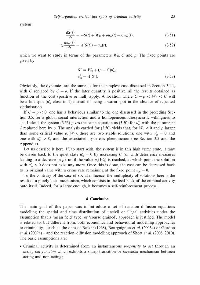
system:

dS(t)

dt= −S(t) + W0 + ρum(t) − Cum(t), (3.51)

τudum(t)

dt= Λ(S(t)) − um(t), (3.52)

which we want to study in terms of the parameters W0, C and ρ. The fixed points are

given by

S∗ = W0 + (ρ − C)u∗m,

u∗m = Λ(S∗). (3.53)

Obviously, the dynamics are the same as for the simplest case discussed in Section 3.1.1,

with C replaced by C − ρ. If the later quantity is positive, all the results obtained as

function of the cost (positive or null) apply. A location where C − ρ < W0 < C will

be a hot spot (u∗m close to 1) instead of being a warm spot in the absence of repeated

victimisation.

If C − ρ < 0, one has a behaviour similar to the one discussed in the preceding Sec-

tion 3.5, for a global social interaction and a homogeneous idiosyncratic willingness to

act. Indeed, the system (3.53) gives the same equation as (3.50) for u∗m with the parameter

J replaced here by ρ. The analysis carried for (3.50) yields that, for W0 < 0 and ρ larger

than some critical value ρc(W0), there are two stable solutions, one with u∗m = 0 and

one with u∗m > 0, and the associated hysteresis phenomenon (see Section 3.5 and the

Appendix).

Let us describe it here. If, to start with, the system is in this high crime state, it may

be driven back to the quiet state u∗m = 0 by increasing C (or with deterrence measures

leading to a decrease in ρ), until the value ρc(W0) is reached, at which point the solution

with u∗m > 0 does not exist any more. Once this is done, the cost can be decreased back

to its original value with a crime rate remaining at the fixed point u∗m = 0.

To the contrary of the case of social influence, the multiplicity of solutions here is the

result of a purely local mechanism, which consists in the feed-back of the criminal activity

onto itself. Indeed, for ρ large enough, it becomes a self-reinforcement process.

4 Conclusion

The main goal of this paper was to introduce a set of reaction–diffusion equations

modelling the spatial and time distribution of uncivil or illegal activities under the

assumption that a ‘mean field’ type, or ‘coarse grained’, approach is justified. The model

is related to, but different from, both economics and behavioural modelling approaches

to criminality – such as the ones of Becker (1968), Bourguignon et al. (2003a) or Gordon

et al. (2009a) – and the reaction–diffusion modelling approach of Short et al. (2008, 2010).

The basic assumptions are:

• Criminal activity is determined from an instantaneous propensity to act through an

acting out function which exhibits a sharp transition or threshold mechanism between

acting and non-acting;


• Locations are characterised by an idiosyncratic willingness to act which introduces

inhomogeneity in the model;

• To represent deterrence, a cost is introduced which represents the law enforcement

presence and efficiency, as well as severity of punishment;

• Social interaction is taken into account by diffusion (both local and non-local) as well

as through a global term;

• A further aspect of deterrence is introduced through local social interaction going in

the opposite direction to the local willingness to act;

• Deterrence and idiosyncratic willingness to act have their own dynamics. In particular,

locations that have high levels of criminality in the past are described by an idiosyncratic

willingness to act which becomes higher and therefore induces more criminal activity

(repeat offences).

This model is discussed in this paper and some particular cases are precisely investigated.

The main conclusions that we can derive from the analysis of these cases are as follows.

There are always stable equilibria, but according to the parameters, multiple stable

equilibria can arise as well. This gives rise to hysteresis-type phenomena.

An important result coming from the analysis of the simplest version of the model

is the existence of a self-organised critical state, where a positive but not large illegal

activity is sustained with the instantaneous propensity to act maintained at a value close

to zero (the critical value below which there is no illegal activity). This may correspond

to two different situations. One is the case of a neighbourhood where the values of the

idiosyncratic propensities to act are large, but where the cost imposed by law enforcement

and deterrence is high enough in order to keep the level of criminal activity under control.

What would be otherwise a hot spot is limited to what we call a warm spot. The other

situation corresponds to a general mode, pervasive through most locations and gives rise

to what we call a tepid milieu. We believe that this is, in particular, a relevant model

for uncivil behaviour, in which case it is reasonable to assume that the idiosyncratic

propensity to act is positive and small almost everywhere (with possibly quiet spots of

negative values and hot spots of high values).

We have also discussed optimal policy issues under the constraint of limited resources

in law enforcement and deterrence. We have shown that a simple adaptive scheme allows

to enforce the optimal policy, limiting as much as possible the average criminal activity,

with most if not all hot spots being reduced to warm spots.

Finally, the consequences of repeated victimisation have been only explored here in the

simplest setting. Some warm spots may, unsurprisingly, become hot spots when repeated

victimisation is taken into account. In such case, within our framework the only way to

reduce such a hot spot to a warm spot is to increase the cost or take deterrent measures

leading to a decrease of the strength of repeated victimisation. Another consequence is

the appearance of multiple stable equilibria: locations where one would not expect to see

a high criminal activity may become hot spots due to the self-reinforcement mechanism.

These hot spots can be reduced through a temporary increase of the cost, taking advantage

of the hysteresis phenomenon.


Many aspects have not been analysed in details in the present paper, and we propose

our model for further mathematical investigation. As of matter of fact, it opens the way to

many new problems. Of particular interest will be the study of the interplay between the

repeated victimisation effect (increase of the idiosyncratic propensity to act at locations

subject to recent illegal activity), and of social interaction (diffusion of the propensity to

act). It remains to see if diffusion of hot spots, or oscillating behaviour may emerge. It

would be interesting to see whether this model produces, as in Short et al. (2010), the

possibility that owing to the action of police on one hot spot, it might be displaced to be

reformed elsewhere. In fact, here we could be more precise and ask if two locations could

swap their natures, oscillating between warm and hot states as triggered by crackdowns

by the police. Indeed, as a result of adapting deterrence, oscillating behaviour might

emerge. This would shed a new light on the nature of reformation of hot spots and could

account for why this phenomena might be underestimated in the statistics. Actually, we

conjecture that often, rather than being displaced and forming entirely new hot spots, the

displacement might just enhance already existing warm spots.

Acknowledgements

This work benefited from discussions with criminologists met a the IPAM workshop

‘Crime Hot Spots: Behavioral, Computational and Mathematical Models’, UCLA 2007,

at the Dahlem Konferenz ‘Is There a Mathematics of Social Entities?’, Berlin 2008 and

at the Workshop on ‘Mathematical Models of Urban Criminality’, Pisa 2008 – notably

P. J. Brantingham, J. Eck, H. Elffers, M. Felson, S. Johnson, D. Nagin and G. Tita. JPN

thanks V. Semeshenko, J. R. Iglesias and most particularly M. B. Gordon for many fruitful

discussions. We thank the referees as well as M. Felson and S. Johnson for useful remarks

on the manuscript.

HB is Professor (Directeur d’etudes) at EHESS, Paris. JPN is Director of research at

CNRS. This work has been supported by the French Ministry of Research, grant PPF

(Plan Pluri-Formations) ‘Complex Systems in Social Sciences’, and by the programme

SYSCOMM of the French National Research Agency (project ‘DyXi’, grant ANR-08-

SYSC-008).

Appendix A Global social influence: Fixed point solutions

The goal of this appendix is to briefly discuss the existence and multiplicity of solutions

of the fixed point equations in the case of a global social influence (see Section 3.5). This

will be done in terms of the following parameters: the slope β, the cost C , the parameters

characterising the distribution of the idiosyncratic willingness to act and the strength J

of the global social interaction.

As in the rest of this paper, we are interested in the nature of the solutions for a family

of acting out functions indexed by the slope β at S = 0+, with Λ(S) = 0 for S < 0 and

Λ a smooth (say C1) strictly increasing function for S > 0. For what concerns P (W ), we

consider a family of distributions parametrised by the mean value W and the variance

σ2W . One can see from the equations that there is an arbitrary scale: if σW � 0, by a

rescaling of β, C and J , without loss of generality one can assume σW = 1. If σW = 0,


that is, if W takes the same value W everywhere, the set of free parameters reduces to

{β(J − C), βW }.Let us first discuss the simplest case of a homogeneous value of W , hence P (W ) =

δ(W − W ). Then at the fixed point of the dynamics all quantities are homogeneous, and

the fixed point equation for the average crime activity (which is also the activity at any

location) is simply given by

u = Λ(W + (J − C)u). (A 1)

If one assumes the acting out function to be concave on �+, with β = Λ′(S = 0+) =

maxS�0 Λ′(S), one gets (i) a unique solution u > 0 for W > 0; (ii) for W = 0, a unique

solution u = 0 for J − C < 1/β, and two solutions for J > Jc = C + 1/β; and (iii) for

W < 0, there exists a line Jc(W ) � Jc = Jc(0) such that for J < Jc(W ) there is a unique

solution u = 0, and for J > Jc(W ) there exist three solutions (0 which is always stable,

an unstable solution and another stable solution which is positive). In the parameter

space (J,W ), the domain with multiple solutions, which lies in the half-plane J > Jc, is

delimited above by the half-line {J � Jc,W = 0}, and below by the curve J = Jc(W ). For

the particular acting out function (2.2), the critical line J = Jc(W ) is given by

−βW + 1 = β(J − C) − ln β(J − C). (A 2)

Figure 6 shows the domain of multiple solution in the parameter space, which here is

{β(J − C), βW }.In the general case, that is, for a non-homogeneous distribution of W , as we have seen

if we can compute u∗m = u∗ at the fixed point, we have the solution for any x. The average

illegal activity u∗m is obtained as solution of the fixed point equation (3.49), which we

rewrite here, in a slightly different form, as an integral over the distribution of W values,

P (W ) =∫Ωδ(W − W (x))p(x)dx (Figure 3 shows the pdf P (W ) for the spatial pattern

W (x) of Figure 4):

u∗m =

∫ΛC(W + Ju∗

m)P (W ) dW. (A 3)

The analysis of this fixed point equation (A 3) can be done as in Gordon et al. (2009b).

One then expects the nature of the solutions to depend in particular on the smoothness

of the distribution P (W ) and on the number of its maxima. It is convenient to write

W = W + w and P (W ) dW = P0(w) dw where P0 has zero mean and unit variance.

To start with, recall the definition of ΛC : it is defined by ΛC(S) = 0 for S � 0, and

for S > 0 as the inverse of (Λ−1 + C Id) (with here Λ−1 the inverse of the function Λ

restricted to �+). Now let

ΛC (s) ≡∫

ΛC(w + s)P0(w) dw (A 4)

and let ΦC be the inverse of ΛC :

u = ΛC (s) ⇔ s = ΦC (u), (A 5)

where ΦC (u) is a monotonous, increasing, function of u, with limu→1 ΦC (u) = +∞, and,

if P0(w) has a non-bounded support, limu→0 ΦC (u) = −∞, or, if the support of P0(w) is

[wmin, wmax], limu→0 ΦC(u) = −wmax.


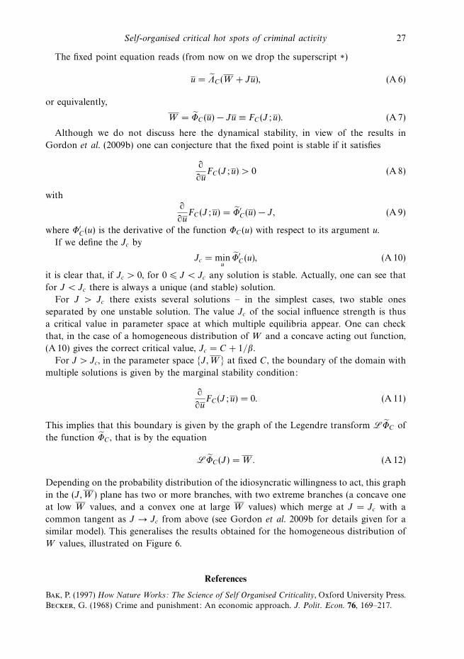
The fixed point equation reads (from now on we drop the superscript ∗)

u = ΛC(W + Ju), (A 6)

or equivalently,

W = ΦC(u) − Ju ≡ FC(J; u). (A 7)

Although we do not discuss here the dynamical stability, in view of the results in

Gordon et al. (2009b) one can conjecture that the fixed point is stable if it satisfies

∂

∂uFC(J; u) > 0 (A 8)

with∂

∂uFC (J; u) = Φ′

C (u) − J, (A 9)

where Φ′C(u) is the derivative of the function ΦC(u) with respect to its argument u.

If we define the Jc by

Jc = minu

Φ′C (u), (A 10)

it is clear that, if Jc > 0, for 0 � J < Jc any solution is stable. Actually, one can see that

for J < Jc there is always a unique (and stable) solution.

For J > Jc there exists several solutions – in the simplest cases, two stable ones

separated by one unstable solution. The value Jc of the social influence strength is thus

a critical value in parameter space at which multiple equilibria appear. One can check

that, in the case of a homogeneous distribution of W and a concave acting out function,

(A 10) gives the correct critical value, Jc = C + 1/β.

For J > Jc, in the parameter space {J,W } at fixed C , the boundary of the domain with

multiple solutions is given by the marginal stability condition:

∂

∂uFC(J; u) = 0. (A 11)

This implies that this boundary is given by the graph of the Legendre transform LΦC of

the function ΦC , that is by the equation

LΦC (J) = W. (A 12)

Depending on the probability distribution of the idiosyncratic willingness to act, this graph

in the (J,W ) plane has two or more branches, with two extreme branches (a concave one

at low W values, and a convex one at large W values) which merge at J = Jc with a

common tangent as J → Jc from above (see Gordon et al. 2009b for details given for a

similar model). This generalises the results obtained for the homogeneous distribution of

W values, illustrated on Figure 6.

References

Bak, P. (1997) How Nature Works: The Science of Self Organised Criticality, Oxford University Press.

Becker, G. (1968) Crime and punishment: An economic approach. J. Polit. Econ. 76, 169–217.


Berk, R. (2008) How you can tell if the simulations in computational criminology are any good.

J. Exp. Criminol. 4(3), 289–308.

Bernasco, W. (2009) Modeling micro-level crime location choice: Application of the discrete choice

framework to crime at places. J. Quant. Criminol. 26(1), 113–138.

Bourguignon, F., Nunez, J. & Sanchez, F. (2003a) A structural model of crime and inequality in

Colombia. J. Eur Econ. Assoc. 12(2–3), 440–449.

Bourguignon, F., Nunez, J. & Sanchez, F. (2003b) What part of the income distribution

does matter for explaining crime? The case of Colombia. J. Eur. Econ. Assoc. 1(2–3), 440–

449.

Brunel, N. & van Rossum, M. C. W. (2007) Lapicques 1907 paper: From frogs to integrate-and-fire.

Bio. Cybern. 97(5–6), 337–339.

Calvo-Armengol, A. & Zenou, Y. (2004) Social networks and crime decisions: The role of social

structure in facilitating delinquent behavior. Int. Econ. Rev. 45, 939–958.

Campbell, M. & Ormerod, P. (1998) Social interactions and the dynamics of crime. Volterra

Consulting Preprint. URL: http://www.paulormerod.com/pdf/CRIME42.pdf

Chow, C., Gutkin, B., Hansel, D., Meunier, C. & Dalibard, J. (editors) (2004) Methods and

Models in Neurophysics. Session LXXX, Lecture Notes of the Les Houches Summer School 2003,

Elsevier.

Clarke, R. V. & Felson, M. (editors) (1993) Routine Activity and Rational Choice. Advances in

Criminological Theory, Vol. 5, Transaction Books, New Brunswick, NJ.

Cohen, L. E. & Felson, M. (1979) Social change and crime rate trends: A routine activity approach.

Am. Sociol. Rev. 44, 588–608.

Crane, J. (1991) The epidemic theory of ghettos and neighborhood effects on dropping out and

teenage childbearing. Am. J. Sociol. 96(5), 1226–1259.

Eck, J. & Liu, L. (2008) Contrasting simulated and empirical experiments in crime. J. Exp. Criminol.

4, 195–213.

Glaeser, E. L., Sacerdote, B. & Scheinkman, J. A. (1996) Crime and social interactions. Q. J.

Econ. 111, 507–548.

Gordon, M. B. (2010) A random walk in the literature on criminality: A partial and

critical view on some statistical analyses and modeling approaches. Eur. J. Appl. Math.,

doi:10.1017/S0956792510000069 (in press).

Gordon, M. B., Iglesias, J. R., Semeshenko, V. & Nadal, J.-P. (2009a) Crime and punishment:

The economic burden of impunity. Eur. Phys. J. B – Condens. Matter Complex Syst. 68(1), 133–

144.

Gordon, M. B., Nadal, J.-P., Phan, D. & Semeshenko, V. (2009b) Discrete choices under social

influence: Generic properties. Math. Models Methods Appl. Sci. (M3AS) 19(Supplementary

Issue 1), 1441–1481.

Groff, L. (2007) Simulation for theory testing and experimentation: An example using routine

activity theory and street robbery. J. Quant. Criminol. 23(2), 75–103.

Johnson, S. D., Summers, L. & Pease, K. (2009) Offender as forager? A direct test of the boost

account of victimization. J. Quant. Criminol. 25(2), 181–200.

Nadal, J.-P., Gordon, M. B., Semeshenko, V. & Iglesias, J. R. (2010) Modelling the

individual and collective dynamics of the propensity to offend. Eur. J. Appl. Math.,

doi:10.1017/S0956792510000173 (in press).

Nadal, J.-P., Phan, D., Gordon, M. B. & Vannimenus, J. (2006) Multiple equilibria in a monopoly

market with heterogeneous agents and externalities. Quant. Finance 5(6), 557–568.

Nagin, D. & Paternoster, R. (1993) Enduring individual differences and rational choice theories

of crime. Law Soc. Rev. 467.

Nuno, J. C., Herrero, M. A. & Primicerio, M. (2008) A triangle model of criminality. Physic. A:

Stat. Mech. Appl. 387(12), 2926–2936.

Ormerod, P. (2005) Crime: Economic Incentives and Social Networks, Insitute of Economic Affairs,

London.


Pease, K. (1998) Repeat victimization: Taking stock. Crime Detection and Prevention Series Paper

90. The Home Office: Police Research Group.

Pitcher, A. B. (2010) Adding police to a mathematical model of burglary. Eur. J. Appl. Math.,

doi:10.1017/S0956792510000112 (in press).

Sethna, J. P. (2009) Statistical Mechanics. Entropy, Order Parameters and Complexity, Oxford Uni-

versity Press.

Short, M. B., Brantingham, P. J., Bertozzi, A. L. & Tita, G. E. (2010) Dissipation and displacement

of hotspots in reaction-diffusion models of crime. Proc. Natl. Acad. Sci. (PNAS) 107(9), 3961–

3965.

Short, M., D’Orsogna, M., Pasour, V., Tita, G., Brantingham, P., Bertozzi, A. & Chayes, L.

(2008) A statistical model of criminal behavior. Math. Models Methods Appl. Sci. (M3AS) 18

(Suppl.), 1249–1267.

self-organised critical hot spots of criminal activitynadal/articles/hotspots.pdfself-organised...

Documents