self-consistent field theory and its applications by m....
TRANSCRIPT

Self-Consistent Field Theoryand Its Applications
by M. W. Matsen
in Soft Matter, Volume 1: Polymer Melts and Mixturesedited by G. Gompper and M. Schick
Wiley-VCH, Weinheim, 2006

Contents
1 Self-consistent field theory and its applications (M. W. Matsen) 31.1 Gaussian Chain . . . . . . . . . . . . . . . . . . . . . . . . . . . . . . . . . 71.2 Gaussian Chain in an External Field . . . . . . . . . . . . . . . . . . . . . . 111.3 Strong-Stretching Theory (SST): The Classical Path . . . . . . . . . . . . . . 151.4 Analogy with Quantum/Classical Mechanics . . . . . . . . . . . . . . . . . . 171.5 Mathematical Techniques and Approximations . . . . . . . . . . . . . . . . 18
1.5.1 Spectral Method . . . . . . . . . . . . . . . . . . . . . . . . . . . . 181.5.2 Ground-State Dominance . . . . . . . . . . . . . . . . . . . . . . . . 201.5.3 Fourier Representation . . . . . . . . . . . . . . . . . . . . . . . . . 211.5.4 Random-Phase Approximation . . . . . . . . . . . . . . . . . . . . . 23
1.6 Polymer Brushes . . . . . . . . . . . . . . . . . . . . . . . . . . . . . . . . 251.6.1 SST for a Brush: The Parabolic Potential . . . . . . . . . . . . . . . 261.6.2 Path-Integral Formalism for a Parabolic Potential . . . . . . . . . . . 281.6.3 Diffusion Equation for a Parabolic Potential . . . . . . . . . . . . . . 311.6.4 Self-Consistent Field Theory (SCFT) for a Brush . . . . . . . . . . . 311.6.5 Boundary Conditions . . . . . . . . . . . . . . . . . . . . . . . . . . 341.6.6 Spectral Solution to SCFT . . . . . . . . . . . . . . . . . . . . . . . 36
1.7 Polymer Blends . . . . . . . . . . . . . . . . . . . . . . . . . . . . . . . . . 411.7.1 SCFT for a Polymer Blend . . . . . . . . . . . . . . . . . . . . . . . 431.7.2 Homogeneous Phases and Macrophase Separation . . . . . . . . . . 451.7.3 Scattering Function for a Homogeneous Blend . . . . . . . . . . . . 471.7.4 SCFT for a Homopolymer Interface . . . . . . . . . . . . . . . . . . 501.7.5 Interface in a Strongly-Segregated Blend . . . . . . . . . . . . . . . 531.7.6 Grand-Canonical Ensemble . . . . . . . . . . . . . . . . . . . . . . 55
1.8 Block Copolymer Melts . . . . . . . . . . . . . . . . . . . . . . . . . . . . . 571.8.1 SCFT for a Diblock Copolymer Melt . . . . . . . . . . . . . . . . . 581.8.2 Scattering Function for the Disordered Phase . . . . . . . . . . . . . 591.8.3 Spectral Method for the Ordered Phases . . . . . . . . . . . . . . . . 611.8.4 SST for the Ordered Phases . . . . . . . . . . . . . . . . . . . . . . 67
1.9 Current Track Record and Future Outlook for SCFT . . . . . . . . . . . . . . 701.10 Beyond SCFT: Fluctuation Corrections . . . . . . . . . . . . . . . . . . . . . 721.11 Appendix: The Calculus of Functionals . . . . . . . . . . . . . . . . . . . . 74Bibliography . . . . . . . . . . . . . . . . . . . . . . . . . . . . . . . . . . . . . 82

2 Contents
Index 83

1 Self-consistent field theory and its applications
M. W. Matsen 1
Department of Physics,University of Reading,Reading, RG6 6AF,United Kingdom
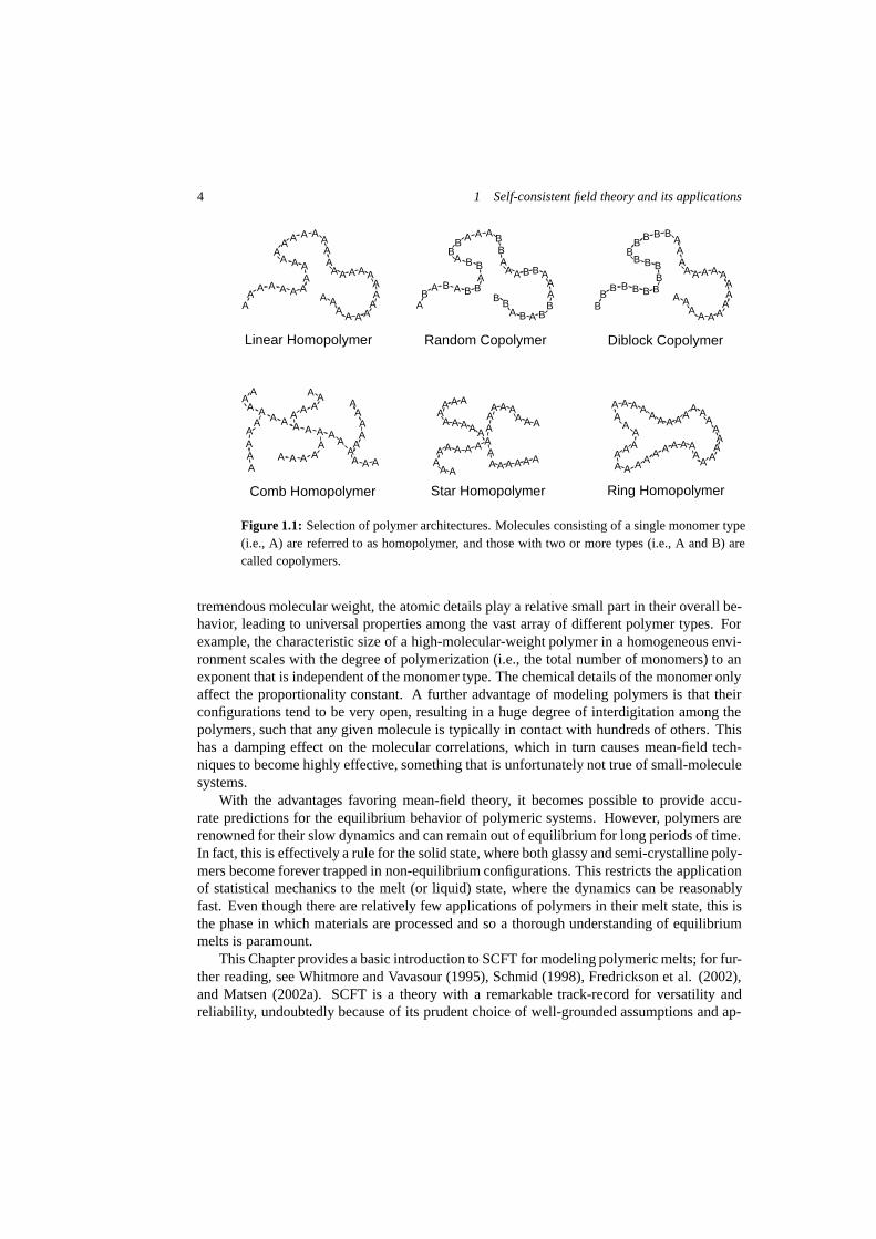
Polymers refer to a spectacularly diverse class of macromolecules formed by covalently link-ing together small molecules, monomers, to form long chains. Figure 1.1 sketches an as-sortment of typical architectures, the simplest of which is the linear homopolymer formedfrom a single strand of identical monomers. There are also copolymer molecules consist-ing of two or more chemically distinct monomer units; the most common example being therandom copolymer, where there is no particular pattern to the monomer sequence. In othercases, the different monomers are grouped together in long intervals to form block copolymermolecules; Fig. 1.1 shows the simplest, a diblock copolymer, formed from one block of A-type units attached to another of B-type units. Although linear chains are the most typical, analmost endless variety of other more elaborate architectures, such as combs, stars and rings,are possible. The monomers themselves also come in a rich variety, some of the more standardof which are listed in Fig. 1.2. The difference in chemistries can have a profound effect on themolecular interactions and chain flexibility. Some monomers produce rigid rod-like polymers,others produce molecules with liquid-crystalline behavior, a few become ionic in solution, andsome are even electrically conducting. The monomer type also has a strong effect on the liquidto solid transition temperature, and influences whether the polymeric material solidifies into aglassy or semi-crystalline state.
As a result of their economical production coupled with their rich and varied properties,polymers have become a vital class of materials for the industrial sector. In addition, someof their exotic behaviors are now being realized for more sophisticated applications in, forexample, the emerging field of nanotechnology. Consequently, research on polymeric macro-molecules has flourished over the past several decades, and now stands as one of the dominantareas in soft condensed matter physics. Through the years of experimental and theoreticalinvestigation, a number of elegant theories have been developed to describe their behavior,and this Chapter is devoted to one of the most successful, self-consistent field theory (SCFT)(Edwards 1965).
Considering the difficulty in modeling systems containing relatively simple moleculessuch as water, one might expect that large polymer molecules would pose an intractable task.However, the opposite is true. The sheer size of these macromolecules (each typically con-taining something like 103 to 105 atoms) actually simplifies the problem. As a result of their
1e-mail address: [email protected]
4 1 Self-consistent field theory and its applications
Linear Homopolymer
AA
A
A
AA
AAA
AAAAA
A A
AAA
A
A
AA
A
A A
AA
A
AA
A
A
Random Copolymer
AB
A
B
BA
BBA
AAABB
A B
ABB
B
A
BB
B
B A
AA
A
AB
B
A
Diblock Copolymer
BB
B
B
BB
BBB
BBBB
BB B
AAA
A
A
AA
A
A A
AA
A
AA
A
A
A
AAAAAAAA
AAAA
AA
AA
A
AA
AAA
A
AA A
A
A
AAA
A
AA
Comb Homopolymer Ring Homopolymer
A
AAAAAAAAA
AA
A
AAA A
A
AA
AA
AA
AA
A AAAA
A A
Star Homopolymer
A A
AAAAAA
A
AAAAA
AAA
AAAA A A A
A
AAAAA A
AA
Figure 1.1: Selection of polymer architectures. Molecules consisting of a single monomer type(i.e., A) are referred to as homopolymer, and those with two or more types (i.e., A and B) arecalled copolymers.
tremendous molecular weight, the atomic details play a relative small part in their overall be-havior, leading to universal properties among the vast array of different polymer types. Forexample, the characteristic size of a high-molecular-weight polymer in a homogeneous envi-ronment scales with the degree of polymerization (i.e., the total number of monomers) to anexponent that is independent of the monomer type. The chemical details of the monomer onlyaffect the proportionality constant. A further advantage of modeling polymers is that theirconfigurations tend to be very open, resulting in a huge degree of interdigitation among thepolymers, such that any given molecule is typically in contact with hundreds of others. Thishas a damping effect on the molecular correlations, which in turn causes mean-field tech-niques to become highly effective, something that is unfortunately not true of small-moleculesystems.
With the advantages favoring mean-field theory, it becomes possible to provide accu-rate predictions for the equilibrium behavior of polymeric systems. However, polymers arerenowned for their slow dynamics and can remain out of equilibrium for long periods of time.In fact, this is effectively a rule for the solid state, where both glassy and semi-crystalline poly-mers become forever trapped in non-equilibrium configurations. This restricts the applicationof statistical mechanics to the melt (or liquid) state, where the dynamics can be reasonablyfast. Even though there are relatively few applications of polymers in their melt state, this isthe phase in which materials are processed and so a thorough understanding of equilibriummelts is paramount.
This Chapter provides a basic introduction to SCFT for modeling polymeric melts; for fur-ther reading, see Whitmore and Vavasour (1995), Schmid (1998), Fredrickson et al. (2002),and Matsen (2002a). SCFT is a theory with a remarkable track-record for versatility andreliability, undoubtedly because of its prudent choice of well-grounded assumptions and ap-

5
Polyethylene (PE)
C C
C H
H
HH
H H
[
CH
H
[
Polypropylene (PP)
C CHH
H H
[ O Polyethyleneoxide (PEO)
C C
ClH
H H
[ Polyvinylchloride (PVC)
C CHH
H H
C[ CH H
Polybutadiene (PB)
Polyisoprene (PI)
Figure 1.2: Chemical structure of some common monomers used to form polymer molecules.
proximations. In most applications, the theory employs the simple coarse-grained Gaussianmodel for polymer chains, and treats their interactions by mean-field theory. Section 1.1 be-gins by justifying the applicability of the Gaussian model, and then Section 1.2 develops thenecessary statistical mechanics for a single chain subjected to an external field, w(r). Follow-ing that, a number of useful approximations are introduced for handling special cases such aswhen w(r) is either weak or strong. This provides the necessary background for discussingSCFT.
As with most theories, the framework of SCFT is best described by demonstrating itsapplication on a representative sample of systems. To this end, we focus on the three exam-ples depicted in Fig. 1.3: polymer brushes, homopolymer interfaces, and block copolymermicrostructures. Not only do they represent a varied range of applications, but they are alsoimportant systems in their own right. A polymeric brush is formed when chains are grafted toa substrate in such high concentration that they create a dense coating with highly extendedconfigurations. Brushes are simple to prepare and provide a convenient way of modifyingthe properties of a surface, and can, for example, greatly reduce friction, change the wettingbehavior, and affect adhesion properties. Polymeric alloys (or blends) provide an economical

6 1 Self-consistent field theory and its applications
Substrate
(a) Polymeric Brush
(b) Homopolymer Interface
(c) Diblock Copolymer Lamellar Phase
D
Figure 1.3: (a) Polymeric brush consisting of polymer chains end-grafted to a flat substrate. (b)Polymer interface separating an A-rich phase (blue domain) from a B-rich phase (red domain).(c) Lamellar diblock copolymer microstructure consisting of alternating thin A- and B-rich do-mains with a repeat period of D.
method of designing new materials with tailored properties. Because large macromoleculespossess relatively little translational entropy, the unlike polymers in an alloy tend to segregatewhile they are being processed in the melt state, leaving the solid material with a domain

1.1 Gaussian Chain 7
structure involving an extensive amount of internal interface. Naturally, the properties of theinterface have a pronounced effect on the final material; in particular, a high interfacial tensionresults in large domains, which is generally undesirable. One way of halting the tendency ofdomains to coarsen is to chemically bond the unlike polymers together, forming block copoly-mer molecules. The blocks still segregate into separate domains, but the connectivity of thechain prevents the domains from becoming thicker than the typical size of a single molecule.In fact, the domains tend to form highly-ordered periodic geometrics, of which the lamellarphase of alternating thin layers pictured in Fig. 1.3(c) is the simplest. This ability to self-assemble into ordered nanoscale morphologies of different geometries is a powerful featurethat researchers are now beginning to exploit for various high-tech applications.
1.1 Gaussian Chain
To start off, we consider linear homopolymer chains in a homogeneous environment, and dis-regard, for the moment, all monomer-monomer interactions including the hard-core ones thatprevent the chains from overlapping. In the limit of high molecular weights, all such polymersfall into the same universality class of non-avoiding random walks, and as a consequence theyexhibit a degree of common behavior. For instance, their typical size scales with their molec-ular weight to the universal exponent, ν = 1/2. To investigate this common behavior, there isno need to consider realistic polymer chains involving segments such as those denoted in Fig.1.2. The fact that the behavior is universal means that it is exhibited by all models, includingsimple artificial ones.
For maximum simplicity, we select the freely-jointed chain, where each monomer has afixed length, b, and the joint between sequential monomers is completely flexible. Figure1.4(a) shows a typical configuration of this model, projected onto the two-dimensional page.It was produced by joining together M = 4000 vectors, r i, each generated from the randomdistribution,
p1(ri) =δ(ri − b)
4πb2(1.1)
where ri ≡ |ri|. The factor in the denominator ensures that the distribution is properly nor-malized such that∫
dr p1(r) = 4π
∫ ∞
0
dr r2p1(r) = 1 (1.2)
The size of the particular configuration displayed in Fig. 1.4(a) can be characterized bythe length of its end-to-end vector,
R ≡M∑i=1
ri (1.3)
denoted by the arrow at the top of the figure. The length of this vector averaged over allpossible configurations, R0, can then be used as a measure for the typical size of the polymer.

8 1 Self-consistent field theory and its applications
(a) m=1
(b) m=16
R
Figure 1.4: (a) Freely-jointed chain with M = 4000 fixed-length monomers. (b) Coarse-grained version with N = 250 segments, each containing m = 16 monomers. The two ends ofthe polymer are denoted by solid dots and the end-to-end vector, R, is drawn above.
Since the simple average, 〈|R|〉, is difficult to evaluate, it is common practice to use thealternative root-mean-square (rms) average,
R0 ≡√〈R2〉 =
√√√√⟨∑i,j
ri · rj
⟩= bM1/2 (1.4)
In this case, the formula conveniently simplifies by the fact, 〈r i · rj〉 = 0 for all i �= j, becausethe directions of different steps are uncorrelated. The power-law dependence on the degreeof polymerization, M , and the exponent, ν = 1/2, are universal properties of non-avoidingrandom walks, and would have occurred regardless of the actual model and the measure usedto characterize the size. The details of the model and the precise definition of size only affectthe proportionality constant, which in this case is simply b.
The underlying reason for the universality of non-avoiding random walks emerges whenthey are examined on a mesoscopic scale, where the chain is viewed in terms of larger repeatunits referred to as coarse-grained segments. For this, new distribution functions, p m(r), aredefined for the end-to-end vector, r, of segments containing m monomers. These distributionfunctions can be evaluated by using the recursive relation,
pm(r) =∫
dr1dr2 pm−n(r1)pn(r2)δ(r1 + r2 − r) (1.5)
where n is any positive integer less than m. By symmetry, each pm(r) depends only on themagnitude, r, of its end-to-end vector, r. This fact combined with the constraint, r 2 = r− r1,can be used to reduce the six-dimensional integral in Eq. (1.5) to the two-dimensional one,
pm(r) = 2π
∫ ∞
0
dr1 r21pm−n(r1)
∫ π
0
dθ sin(θ)pn(r2) (1.6)
over the length of r1 and the angle between r and r1. In terms of r1 and θ, the length of r2 isspecified by the cosine law, r2
2 = r2 + r21 − 2rr1 cos(θ). Using this relation to substitute θ by

1.1 Gaussian Chain 9
r2, the preceding integral can then be expressed in the slightly more convenient form,
pm(r) =2π
r
∫ ∞
0
dr1 r1pm−n(r1)∫ r+r1
|r−r1|dr2 r2pn(r2) (1.7)
With the recursion relation in Eq. (1.7), it is now a straightforward exercise to marchthrough calculating pm(r) for larger and larger segments. Starting with m = 2 and n = 1, thetwo-monomer distribution,
p2(r) ={
18πb2r , if r < 2b0 , if 2b < r
(1.8)
is obtained from the single-step distribution in Eq. (1.1). One can easily confirm that thisdistribution is properly normalized as p1(r) was in Eq. (1.2). Repeating the process withm = 4 and n = 2 gives the four-monomer distribution,
p4(r) =
⎧⎨⎩
8b−3r64πb4 , if r < 2b(4b−r)2
16πb4r , if 2b < r < 4b0 , if 4b < r
(1.9)
Although the formulas become increasingly complicated, it is straightforward to continue theiterations numerically.
Figure 1.4(b) displays an equivalent random walk to that in Fig. 1.4(a), but where eachsegment corresponds to m = 16 monomers with a distribution given by p 16(r). The actof combining m monomers into larger units, or segments, makes the chain appear smootherand buries microscopic degrees of freedom into the probability distribution, p m(r). Thisprocedure, where the number of units is reduced from M down to N ≡ M/m, is referredto as coarse graining. It does away with M and b, and replaces them by N and a statisticalsegment length,
a ≡ R0N−1/2 = bm1/2 (1.10)
defined such that R0 = aN1/2.When the probability distributions, pm(r), are scaled with respect to the statistical segment
length, a, they approach the asymptotic limit,
pm(r) →(
32πa2
)3/2
exp(−3r2
2a2
)(1.11)
as m → ∞. Figure 1.5 demonstrates this by comparing distributions of finite m (solid curves)against the asymptotic limit (dashed curve). This convergence to a simple Gaussian distribu-tion is well known in statistics and goes by the name of the central limit theorem. The Gaus-sian (or normal) distribution applies to the average of any large random sample, in this casethe displacement vectors of m monomers. Even if the lengths of the individual monomerswere not fixed, but varied according to some arbitrary distribution, the coarse-grained seg-ments would still develop Gaussian distributions, albeit with a different expression for a. Thisuniversality occurs because the Gaussian distribution represents a fixed point of the recursion

10 1 Self-consistent field theory and its applications
r/a0.0 0.5 1.0 1.5
p m(r
) a3
0.0
0.1
0.2
0.3
8
16
m=4
Figure 1.5: Probability distribution, pm(r), for a coarse-grained segment with m monomers.The dashed curve denotes the asymptotic limit in Eq. (1.11) for m → ∞.
relation in Eq. (1.5); in other words, if pm−n(r1) and pn(r2) are both Gaussians, then so ispm(r).
This universality actually extends beyond freely-jointed chains to a more general class thatcan be referred to as Markov chains. An equilibrium configuration of a Markov chain can stillbe generated by starting at one end and attaching monomers one-by-one according to a givenprobability distribution. However, in this case, the displacement of the i’th monomer, r i, canhave a distribution, p1(ri; ri−1), that depends on the ri−1 of the preceding monomer. In fact,this can be generalized such that the probability of r i depends on ri−1, ri−2,..., ri−I so longas I remains finite. If this is the case, then sufficiently large coarse-grained segments will stilldevelop a Gaussian distribution with an average chain size obeying R 0 = aN1/2.
While the universality class of random walks applies to an impressive range of models, itdoes not include those with self-avoiding interactions. In that case, the position and orientationof a particular monomer is dependent upon all others in the chain. Nevertheless, such polymerconfigurations can still be generated with random walks, but those configurations contain-ing overlaps must now be disregarded. The smaller compact configurations are more likelyto contain overlapping monomers, and therefore self-avoidance favors larger and more openconfigurations. Consequently, the size of an isolated polymer in solution scales as R 0 ∝ Nν
with a larger exponent of ν ≈ 0.6 (de Gennes 1979). However, when the polymer is in a meltwith other polymers, it has to avoid them as well as itself. In this case, the advantage of themore open configurations is lost, and the polymer reverts back to random-walk statistics withthe Gaussian probability in Eq. (1.11), although with a modified statistical segment length(Wang 1995).
Fetters et al. (1994) provide a library of experimental results for R 0 as a function of

1.2 Gaussian Chain in an External Field 11
molecular weight and bulk mass densities for various common polymer types, such as thosedepicted in Fig. 1.2. Given the chemical composition and thus the molecular weight of amonomer, it is then possible to calculate the statistical segment length, a, and the bulk segmentdensity, ρ0. However, the values obtained depend on the definition of the segment (i.e., thevalue selected for m). Of course, none of the physical quantities can be affected by such achoice, and indeed this is always the case. If, for example, the number of monomers in eachsegment is doubled, then N decreases by a factor of 2 and a increases by
√2, such that the
quantity, R0 = aN1/2, remains unchanged.The freedom to redefine segments is linked to the scaling behavior and thus the universality
of polymeric systems. However, it can be confusing because the size of N no longer has anyabsolute meaning, or in other words, it is impossible to judge whether a polymer is long orshort based solely on its value of N . Fortunately, there is a special invariant definition,
N ≡(
R30
N/ρ0
)2
= a6ρ20N (1.12)
with a real physical significance that provides a true measure of the polymeric nature of themolecule. It is based on the ratio of the typical volume spanned by a polymer, R 3
0, to itsphysical volume, N/ρ0. Thus, small values of N correspond to compact molecules and largevalues imply open configurations with many intermolecular contacts. Be aware that someauthors assume, without mentioning, that N = N by innocuously setting the segment volumeto ρ−1
0 = a3.
1.2 Gaussian Chain in an External Field
The preceding section examined polymers in an ideal homogeneous environment, where noforces were exerted on the chains. In the more interesting situations depicted in Fig. 1.3, thepolymers do experience interactions that vary with respect to position, r. Their net effect cangenerally be represented by a static field, w(r), determined self-consistently from the overallsegment distribution in the system. However, we ignore for now the source of the field andstart by developing the statistical mechanics for a single polymer acted upon by an arbitraryexternal field. Although fields are generally real quantities, the derivations that follow holdeven when w(r) is complex; this fact will be needed in the derivation of self-consistent fieldtheory (SCFT).
We assume that the field varies slowly enough that the chain can be divided into N appro-priately sized coarse-grained segments of volume, ρ−1
0 , each small enough such that their localenvironment is more or less homogeneous, but also large enough so that they obey Gaussianstatistics with a statistical segment length, a. The coarse-grained trajectory of the polymer(e.g., the path in Fig. 1.4(b)) is then specified by a function, rα(s), where the parameter,0 ≤ s ≤ 1, runs along the backbone of the polymer such that equal intervals of s have thesame molecular weight. (The subscript α will be used to label different molecules when weeventually treat complete systems.) Having specified the trajectory, a dimensionless segmentconcentration can be defined as
φα(r) =N
ρ0
∫ 1
0
ds δ(r − rα(s)) (1.13)

12 1 Self-consistent field theory and its applications
The energy of a polymer configuration, rα(s), turns out to be a local property, meaning thatany given interval of the chain, s1 ≤ s ≤ s2, can be assigned a definite quantity of energy,E[rα, s1, s2], independent of the rest of the chain. This will become a crucial property in thederivation that follows. The formula for the energy,
E[rα; s1, s2]kBT
=∫ s2
s1
ds
(3
2a2N|r′α(s)|2 + w(rα(s))
)(1.14)
involves one term that accounts for the Gaussian probability from Eq. (1.11) and another termfor the energy of the field. Note that square brackets are used for E[rα; s1, s2] to denote thatit is a functional (i.e., a function of a function).
The two primary quantities of the polymer that need to be calculated are the ensemble-
averaged concentration, φα(r) ≡⟨φα(r)
⟩, and the configurational entropy, S. In order to
evaluate these, some partition functions are required. To begin, consider the first sN segments(0 ≤ s ≤ 1) of the chain constraining the two ends at rα(0) = r0 and rα(s) = r. The energyof this fragment is E[rα; 0, s] and thus its partition function is
q(r, r0, s) ∝∫
Drα exp(−E[rα; 0, s]
kBT
)δ(rα(0) − r0)δ(rα(s) − r) (1.15)
This is a functional integral over all configurations, rα(t), for 0 < t < s, weighted by theappropriate Boltzmann factor; the delta functions simply exclude those configurations wherethe two ends are not at r0 and r. (Those unfamiliar with functional integrals should refer tothe Appendix.) In principle, the Boltzmann factor in the partition function should also containthe kinetic energy, and the functional integration should also extend over the momenta of allthe monomers. However, the form of the kinetic energy allows the momentum coordinates tobe integrated out and included in the proportionality factor (Hong and Noolandi 1981), whichin any case has been omitted from Eq. (1.15). A proper evaluation of the proportionalityconstant would require a detailed account of the exact degrees of freedom available to all theatoms in the polymer molecule, but such information is lost in the coarse-graining procedure.Fortunately, the proportionality constant has no effect on the evaluation of φ α(r). Although itdoes affect S, it does so simply by an additive constant, which is immaterial since we will onlybe concerned with changes in entropy. Thus, the proportionality relationship in Eq. (1.15) issufficient for our purposes.
The local property of the polymer energy is manifest mathematically by the equality,E[rα; 0, s] = E[rα; 0, t] + E[rα; t, s] for any t ∈ [0, s]. This implies the recursive relation,
q(r, r0, s) =1
(a2N)3/2
∫dr1 q(r, r1, t)q(r1, r0, s − t) (1.16)
which gives the partition function for a fragment of sN segments in terms of the partitionfunctions of two shorter fragments. By including an equality sign in Eq. (1.16), we haveeffectively chosen a value for the missing proportionality factor in Eq. (1.15); not one that hasany actual meaning, but merely the simplest one that renders q(r, r 0, s) dimensionless. Thisrecursion relation also implies
q(r, r0, 0) = (a2N)3/2δ(r − r0) (1.17)

1.2 Gaussian Chain in an External Field 13
because Eq. (1.16) must hold for t → 0. Naturally q(r, r0, 0) = 0 when r �= r0, since s = 0implies that r and r0 both correspond to the same point on the chain.
The recursion relation, Eq. (1.16), provides a means of building up the partition functionfor a long chain fragment from those of very short fragments. This reduces the problem tothe easier one of finding q(r, r0, ε), where ε is small enough that the field can be treated as aconstant for typical chain extensions of |r − r0| � a(εN)1/2. In this case, the field simplyadds a constant energy of εw(r)kBT to each configuration, and thus does not affect the relativeprobability of its configurations. Therefore, the partition function can be expressed as
q(r, r0, ε) ≈(
32πε
)3/2
exp(−3|r− r0|2
2a2Nε− εw(r)
)(1.18)
which assumes the Gaussian distribution in Eq. (1.11) for a chain of εN segments in a ho-mogeneous environment, adjusted for the constant energy of the field and normalized so thatit reduces to Eq. (1.17) in the limit ε → 0. For extensions, |r − r0|, significantly beyonda(εN)1/2, the partition function approaches zero regardless of whether or not the field energyis well-approximated by εw(r)kBT . Hence, Eq. (1.18) remains accurate over all extensions,provided that a(εN)1/2 is sufficiently small relative to the spatial variations in w(r).
Now the partition function for large fragments can be calculated iteratively using
q(r, r0, s + ε) =1
(a2N)3/2
∫drε q(r, r + rε, ε)q(r + rε, r0, s) (1.19)
The first partition function, q(r, r + rε, ε), under the integral implies that we only need toknow the second one, q(r + rε, r0, ε), accurately for |rε| � a(εN)1/2. We therefore expand itin the Taylor series,
q(r, r0, s + ε) =1
(a2N)3/2
∫drε q(r, r + rε, ε) ×[1 + rε · ∇ +
12rεrε : ∇∇
]q(r, r0, s) (1.20)
to second order in rε. Here, we have used the dyadic notation (Goldstein 1980) for the second-order term. The expansion now makes it possible to explicitly integrate over r ε, giving
q(r, r0, s + ε) ≈ exp (−εw(r))[1 +
a2N
6ε∇2
]q(r, r0, s) (1.21)
≈[1 +
a2N
6ε∇2 − εw(r)
]q(r, r0, s) (1.22)
to first order in ε. Alternatively, a Taylor-series expansion in s gives
q(r, r0, s + ε) ≈[1 + ε
∂
∂s
]q(r, r0, s) (1.23)
By direct comparison, it immediately follows that
∂
∂sq(r, r0, s) =
[a2N
6∇2 − w(r)
]q(r, r0, s) (1.24)

14 1 Self-consistent field theory and its applications
which is the modified diffusion equation normally used to evaluate q(r, r 0, s). Likewise, apartial partition function,
q(r, s) ∝∫
Drα exp(−E[rα; 0, s]
kBT
)δ(rα(s) − r) (1.25)
can be defined for a chain fragment with a free s = 0 end. The fact that
q(r, s) =1
(a2N)3/2
∫dr0 q(r, r0, s) (1.26)
implies that it also satisfies Eq. (1.24), given that the diffusion equation is linear. Furthermore,Eq. (1.17) implies the initial condition, q(r, 0) = 1.
In a completely analogous way, complementary partition functions are defined for the last(1 − s)N segments of the chain. The one for a fixed s = 1 end is defined as
q†(r, r0, s) ∝∫
Drα exp(−E[rα; s, 1]
kBT
)δ(rα(s) − r)δ(rα(1) − r0) (1.27)
and satisfies the diffusion equation,
∂
∂sq†(r, r0, s) = −
[a2N
6∇2 − w(r)
]q†(r, r0, s) (1.28)
subject to the condition, q†(r, r0, 1) = (a2N)3/2δ(r − r0). For an unconstrained end, thecomplementary partition function becomes
q†(r, s) =1
(a2N)3/2
∫dr0 q†(r, r0, s) (1.29)
satisfying Eq. (1.28) with q†(r, 1) = 1. The full partition function, Q[w], for a polymer inthe field, w(r), is then related to the integral of the two partial partition functions. In the casewhere both ends of the polymer are free,
Q[w] =∫
dr q(r, s)q†(r, s) ∝∫
Drα exp(−E[rα; 0, 1]
kBT
)(1.30)
Again, the square brackets on Q[w] denote that it is a functional that depends on the function,w(r).
With the partition functions in hand, the average segment distribution, φ α(r), can nowbe evaluated. Here the calculation is shown for an unconstrained polymer, but the proce-dure is essentially the same if one or both ends are constrained. Following standard statisticalmechanics, the average is computed by weighting each configuration by the appropriate Boltz-mann factor;
φα(r) =1
Q[w]
∫Drαφα(r) exp
(−E[rα; 0, 1]
kBT
)
=N
ρ0Q[w]
∫ 1
0
ds
∫Drαδ(r − rα(s)) exp
(−E[rα; 0, 1]
kBT
)
=N
ρ0Q[w]
∫ 1
0
ds q(r, s)q†(r, s) (1.31)

1.3 Strong-Stretching Theory (SST): The Classical Path 15
This equation provides the practical means of calculating the average segment concentration,but there will also be instances where we need to identify it by the functional derivative,
φα(r) = −N
ρ0
D ln(Q[w])Dw(r)
≡ −N
ρ0limε→0
ln(Q[w + εδ]) − ln(Q[w])ε
(1.32)
The equivalence of this functional derivative to Eq. (1.31) follows almost immediately fromthe alternative expression,
Q[w] ∝∫
Drα exp(− 3
2a2N
∫ 1
0
ds|r′α(s)|2 − ρ0
N
∫dr1 w(r1)φα(r1)
)(1.33)
for the partition function. Note that Q[w+ εδ] simply refers to the partition function evaluatedwith w(r1) replaced by w(r1) + εδ(r1 − r). (See the Appendix for further information onfunctional differentiation.)
Lastly, we calculate the entropy, S, or equivalently the entropic free energy, f e ≡ −TS,which, for reasons that will become apparent, is also called the elastic free energy of thepolymer. In accord with standard statistical mechanics, the entropic energy is
fe
kBT= − ln
(Q[w]V
)− ρ0
N
∫dr w(r)φα(r) (1.34)
The logarithm of Q[w] gives the total free energy of the polymer in the field, while the integralremoves the average internal energy acquired from the field, leaving behind the entropic en-ergy. The extra factor of V in the logarithm simply adds a constant to f e such that the entropicenergy is measured relative to the homogeneous state; it is easily confirmed that Eq. (1.34)gives fe = 0 for the case of a uniform field.
Since the force exerted on the segments is given by the gradient of the field, an additiveconstant to the field should have no effect on any physical quantities. Indeed, this is the case.If a constant, w0, is added to the field such that w(r) ⇒ w(r) + w0, the partition functionstransform as
q(r, s) ⇒ q(r, s) exp(−sw0) (1.35)
q†(r, s) ⇒ q†(r, s) exp(−(1 − s)w0) (1.36)
Q[w] ⇒ Q[w] exp(−w0) (1.37)
When these substitutions are entered into Eq. (1.31), all the exponential factors cancel, leavingφα(r) unaffected. Likewise, w0 cancels out of Eq. (1.34) for fe, using the fact that the averagesegment concentration is φα = N/ρ0V . This invariance will generally be used to set thespatial average of the field, w, to zero.
1.3 Strong-Stretching Theory (SST): The Classical Path
In circumstances where the field energy becomes large relative to the thermal energy, k BT ,the polymer is effectively restricted to those configurations close to the ground state, referredto as the classical path for reasons that will become apparent in the following section. This

16 1 Self-consistent field theory and its applications
opens up the possibility of low-temperature series approximations, but one first needs to locatethe ground-state trajectory by minimizing
E[rα; 0, 1] =∫ 1
0
dsL(rα(s), r′α(s)) (1.38)
where
L(rα(s), r′α(s)) ≡ 32a2N
|r′α(s)|2 + w(rα(s)) (1.39)
This is a standard calculus of variations problem, which, as demonstrated in the Appendix, isequivalent to solving the Euler-Lagrange equation,
d
ds
(∂L∂r′α
)− ∂L
∂rα= 0 (1.40)
This is a slight generalization of Eq. (1.331), due to the fact that rα(s) is a vector rather thana scalar function. Nevertheless, the differentiation of L in Eq. (1.40) is easily performed andleads to the differential equation,
3a2N
r′′α(s) −∇w(rα(s)) = 0 (1.41)
Solving this vector equation subject to possible boundary conditions for r α(0) and rα(1)provides the classical path.
Although Eq. (1.41) is sufficient, we can derive an alternative equation that provides auseful relation between the local chain extension, |r ′
α(s)|, and the field energy, w(rα(s)).This is done by dotting Eq. (1.41) with r ′
α(s) to give
3a2N
r′α(s) · r′′α(s) − r′α(s) · ∇w(rα(s)) = 0 (1.42)
which, in turn, can be rewritten as
d
ds
(3|r′α(s)|2
2a2N
)− d
dsw(rα(s)) = 0 (1.43)
Performing an integration reduces this to the first-order differential equation,
3|r′α(s)|22a2N
− w(rα(s)) = constant (1.44)
In cases of appropriate symmetry, the classical trajectory can be derived from this scalar equa-tion alone.
Once the classical path is known, the average segment concentration is given by
φα(r) =N
ρ0
∫ 1
0
ds δ(r − rα(s)) (1.45)
and the entropic free energy is
fe
kBT=
32a2N
∫ 1
0
ds |r′α(s)|2 (1.46)
This entropic energy is often referred to as the elastic or stretching energy, because it has theequivalent form to the stretching energy of a thin, elastic thread.

1.4 Analogy with Quantum/Classical Mechanics 17
1.4 Analogy with Quantum/Classical Mechanics
Every so often, mathematics and physics are bestowed with a powerful mapping that equatestwo diverse topics. In one giant leap, years of accumulated knowledge on one topic canbe instantly transferred to another. Here, we encounter such an example by the fact that aGaussian chain in an external field maps onto the quantum mechanics of a single particle in apotential. For those without a background in quantum mechanics, the section can be skimmedover without seriously compromising one’s understanding of the remaining sections.
The mapping becomes apparent when examining the path-integral formalism of quantummechanics introduced by Feynman and Hibbs (1965). With incredible insight, they demon-strate that the quantum mechanical wavefunction, Ψ(r, t), for a particle of mass, m, in apotential, U(r), is given by the path integral,
Ψ(r, t) =∫
Drp exp(iS/�)δ(rp(t) − r) (1.47)
over all possible trajectories, rp(t), where the particle terminates at position, r, at time, t.(Note that i ≡ √−1.) In this definition, each trajectory contributes a phase factor given by theclassical action,
S ≡∫
dt[m
2|r′p(t)|2 − U(rp(t))
](1.48)
which, in this case, is kinetic energy minus potential energy integrated along the particletrajectory. Naturally, Feynman justified this by showing that Eq. (1.47) is equivalent to theusual time-dependent Schrodinger equation,
i�∂
∂tΨ(r, t) =
[− �
2
2m∇2 + U(r)
]Ψ(r, t) (1.49)
in much the same way Section 1.2 derived the diffusion equation for q(r, s).Taking a closer look, the mathematics of this quantum mechanical problem is exactly that
of our polymer in an external field. A precise mapping merely requires the associations,
t ⇔ s (1.50)
m ⇔ 3a2N
(1.51)
U(r) ⇔ −w(r) (1.52)
S ⇔ E[rα; 0, s]kBT
(1.53)
rp(t) ⇔ rα(s) (1.54)
� ⇔ −i (1.55)
Ψ(r, t) ⇔ q(r, s) (1.56)
Indeed, these substitutions transform Eq. (1.47) for the wavefunction into Eq. (1.25) for thepartition function of sN polymer segments, and likewise the Schrodinger Eq. (1.49) trans-forms into the diffusion Eq. (1.24).

18 1 Self-consistent field theory and its applications
Extending this analogy further, the strong-stretching theory (SST) developed in Section1.3 is found to be equivalent to classical mechanics. In Feynman’s formulation, the connec-tion between quantum mechanics and classical mechanics becomes exceptionally transparent.When the action, S, of a particle is large relative to �, the path integral becomes dominated bythe extremum of S, because all paths close to the extremum contribute the same phase factor,and thus add constructively. (This is the basis of Fermat’s principle in optics by which thefull wave treatment of light can be reduced to classical ray optics (Hecht and Zajac 1974).)However, the procedure of finding the extremum of S is precisely the Lagrangian formalismof classical mechanics (Goldstein 1980). Thus, in the limit of large S, the particle follows theclassical mechanical trajectory determined by Newton’s equation of motion (i.e, ma = F),
mr′′p(t) = −∇U(rp(t)) (1.57)
Equally familiar in classical mechanics is the equation for the conservation of energy,
m
2|r′p(t)|2 + U(rp(t)) = constant (1.58)
In terms of the analogy, classical mechanics corresponds to the case where E[rα; s1, s2]/kBTis large relative to one, which is the condition for the strong-stretching theory (SST) discussedin the preceding section. Indeed, Eq. (1.57) matches precisely with Eq. (1.41) for the ground-state polymer trajectory, as does Eq. (1.58) with Eq. (1.44). It is this analogy from which theground-state trajectory acquires its name, the classical path.
1.5 Mathematical Techniques and Approximations
Quantum mechanics has experienced a massive activity of research since its introduction mid-way through the last century. The accumulated knowledge is staggering, and the fact that ourproblem maps onto it means that we can make significant progress without having to reinventthe wheel. This section demonstrates several useful calculations that draw upon what are nowstandard techniques in quantum mechanics.
1.5.1 Spectral Method
One of the most widely used and fruitful techniques in quantum mechanics is the spectralmethod for solving the time-dependent wavefunction, Ψ(r, t). Here, the method is adapted tothe evaluation of the partial partition functions, q(r, s) and q †(r, s), for a homopolymer in anexternal field, w(r). The first step is to solve the analog of the time-independent Schrodingerequation,[
a2N
6∇2 − w(r)
]fi(r) = −λifi(r) (1.59)
for all the eigenvalues, λi, and eigenfunctions, fi(r), where i = 0,1,2,... For reasons that willbe discussed at the end of this section, the eigenvalues are ordered from smallest to largest. As

1.5 Mathematical Techniques and Approximations 19
in quantum mechanics, the eigenfunctions are orthogonal and can be normalized to satisfy,
1V
∫dr fi(r)fj(r) = δij (1.60)
where V is the total volume of the system. Furthermore, the eigenfunctions form a completebasis, which implies that any function of position, g(r), can be expanded as
g(r) =∞∑
i=0
gifi(r) (1.61)
The coefficients, gi, of the expansion are determined by multiplying Eq. (1.61) by f j(r),integrating over r, and using the orthonormal condition from Eq. (1.60). This gives theformula,
gi =1V
∫drfi(r)g(r) (1.62)
Once the orthonormal basis functions have been obtained, it is a trivial matter to evaluateq(r, s). One starts by expanding it as
q(r, s) =∞∑
i=0
qi(s)fi(r) (1.63)
and substituting the expansion into Eq. (1.24). Given the inherent property of the eigenfunc-tions, Eq. (1.59), the diffusion equation reduces to
∞∑i=0
q′i(s)fi(r) = −∞∑
i=0
λiqi(s)fi(r) (1.64)
With the same steps used to derive Eq. (1.62), it follows that
q′i(s) = −λiqi(s) (1.65)
for all i = 0,1,2,.... Differential equations do not come any simpler. Inserting the solution intoEq. (1.63) gives the final result,
q(r, s) =∞∑
i=0
ci exp(−λis)fi(r) (1.66)
where the constant,
ci ≡ qi(0) =1V
∫dr fi(r)q(r, 0) (1.67)
is determined by the initial condition. Similarly, the expression for the complementary parti-tion function is
q†(r, s) =∞∑
i=0
c†i exp(−λi(1 − s))fi(r) (1.68)

20 1 Self-consistent field theory and its applications
where
c†i =1V
∫dr fi(r)q†(r, 1) (1.69)
In practice, it is impossible to complete the infinite sums in Eqs. (1.66) and (1.68), but theeigenvalues are appropriately ordered such that the terms become less and less important.Therefore, the sums can be truncated at some point, i = M , where the number of termsretained, M + 1, is guided by the desired level of accuracy.
1.5.2 Ground-State Dominance
The previous expansion for q(r, s) in Eq. (1.66) becomes increasingly dominated by the firstterm involving the ground-state eigenvalue, λ0, the further s is from the end of the chain. Fora high-molecular-weight polymer, the approximations,
q(r, s) ≈ c0 exp(−λ0s)f0(r) (1.70)
and
q†(r, s) ≈ c†0 exp(−λ0(1 − s))f0(r) (1.71)
become accurate over the vast majority of the chain. In this case, it follows that the partitionfunction of the entire chain is
Q[w] ≈ Vc0c†0 exp(−λ0) (1.72)
and that the segment concentration is
φα(r) ≈ N
ρ0V f20 (r) (1.73)
These simplifications permit us to derive an analytical Landau-Ginzburg free energy expres-sion for the entropic energy, fe, of the polymer as a function of its concentration profile,φα(r). Our derivation will assume that concentration gradient,
∇φα(r) =2N
ρ0V f0(r)∇f0(r) (1.74)
is zero at the extremities (i.e., boundaries) of our system, V .The first step of the derivation is to multiply Eq. (1.59) for i = 0 by f 0(r) and integrate
over V , producing the result,
ρ0
N
∫dr w(r)φα(r) =
a2N
6V∫
dr f0(r)∇2f0(r) + λ0 (1.75)
Next, this expression for the field energy along with Eq. (1.72) for Q[w] are inserted into Eq.(1.34) giving the expression,
fe
kBT= −a2N
6V∫
dr f0(r)∇2f0(r) − ln(c0c†0) (1.76)

1.5 Mathematical Techniques and Approximations 21
for the entropic free energy. The logarithmic term can be dropped in the large-N limit. Anintegration by parts is then performed to reexpress the equation as
fe
kBT=
a2N
6V∫
dr |∇f0(r)|2 (1.77)
where the boundary term vanishes as a result of the assumption, ∇φα(r) = 0, along the edgeof V . For the final step of the derivation, the eigenfunction, f 0(r), is replaced by the segmentconcentration, φα(r), using Eqs. (1.73) and (1.74). This produces the Landau-Ginzburg freeenergy expression,
fe
kBT=
a2ρ0
24
∫dr
|∇φα(r)|2φα(r)
(1.78)
which gives the entropic energy without the need to evaluate the underlying field, w(r). Thederivation assumes only that the molecular weight (i.e., N ) of the polymer is large.
1.5.3 Fourier Representation
Quantum mechanical problems are often made more tractable by reexpressing them in so-called momentum space. The principle is very similar to that of the spectral method, wherequantities are expanded in terms of energy eigenstates. The main difference is that the expan-sions are now in terms of eigenfunctions, exp(ik · r), of the momentum operator, p ≡ −i�∇.(Here, i ≡ √−1.) The other difference is that the momentum eigenvalue, k, is continu-ous, which implies that sums are now replaced by integrals and Kronecker delta functions aresubstituted by Dirac delta functions. For example, the orthogonality condition in Eq. (1.60)becomes
1(2π)3
∫dr exp(i(k1 − k2) · r) = δ(k1 − k2) (1.79)
Furthermore, the expansion of an arbitrary function, g(r), becomes the integral,
g(r) =1
(2π)3
∫dk g(k) exp(ik · r) (1.80)
and the coefficient of the expansion,
g(k) ≡∫
dr g(r) exp(−ik · r) (1.81)
is now a continuous function, referred to as the Fourier transform of g(r). Although g(k)is complex, its complex conjugate satisfies g∗(k) = g(−k), which implies that |g(k)|2 =g(−k)g(k). Before moving on, we quote a useful identity,∫
dr g1(r)g2(r) =1
(2π)3
∫dk g1(−k)g2(k) (1.82)

22 1 Self-consistent field theory and its applications
for the integral of two functions. It can be proved by substituting the expansions for g 1(r) andg2(r) into the left-hand side, identifying the integral over r as the Dirac delta function in Eq.(1.79), and using the sifting property of the delta function from Eq. (1.329).
Now we are ready to Fourier transform the diffusion equation for q(r, s). The first stepis to insert the Fourier representations, Eq. (1.80), of q(r, s) and w(r) into the diffusion Eq.(1.24), giving
∂
∂s
∫dk2q(k2, s) exp(ik2 · r) = −a2N
6
∫dk2k
22q(k2, s) exp(ik2 · r) −
1(2π)3
∫dk1dk2w(k1)q(k2, s) exp(i(k1 + k2) · r) (1.83)
Next the equation is multiplied through by exp(−ik · r) and integrated over r. Using theorthogonality relation in Eq. (1.79), the expression simplifies to
∂
∂s
∫dk2q(k2, s)δ(k2 − k) = −a2N
6
∫dk2k
22q(k2, s)δ(k2 − k) −
1(2π)3
∫dk1dk2w(k1)q(k2, s)δ(k1 + k2 − k) (1.84)
Now we apply the sifting property of the delta function to arrive at the final expression,
∂
∂sq(k, s) = −k2a2N
6q(k, s) − 1
(2π)3
∫dk1w(k1)q(k − k1, s) (1.85)
This equation is then solved for q(k, s) subject to the initial condition
q(k, 0) =∫
dr q(r, 0) exp(−ik · r) (1.86)
For a polymer with a free end,
q(k, 0) = (2π)3δ(k) (1.87)
whereas when the s = 0 end is fixed at r0,
q(k, 0) = (aN1/2)3 exp(ik · r0) (1.88)
In either case, the solution to Eq. (1.85) for a homogeneous environment (i.e., w(r) = 0) isreadily expressed as
q(k, s) = q(k, 0) exp(−k2a2Ns/6) (1.89)
from which q(r, s) immediately follows. The aim of the next section will be to extend thisresult to polymers in a weak field.

1.5 Mathematical Techniques and Approximations 23
1.5.4 Random-Phase Approximation
Here, a Landau-Ginzburg free energy expression is derived for the entropic free energy, f e, of apolymer molecule in a weakly-varying field, w(r). As before in Section 1.5.2, this calculationwill assume that the two ends of the chain are free, by imposing the initial condition in Eq.(1.87). We will also use the invarience discussed at the end of Section 1.2 to fix the spatialaverage of the field to w = 0. Given that w(r) only deviates slightly from zero, it is safe toassume that the ensemble-averaged segment concentration, φα(r), never strays far from itsspatial average,
φα ≡ 1V
∫dr φα(r) =
N
ρ0V (1.90)
The first step is to find an approximate solution for q(k �= 0, s). Since the integral in Eq.(1.85) involves w(k1), which is small, the multiplicative factor of q(k − k1, s) need not beparticularly accurate. Approximating it by q(k − k1, 0) from Eq. (1.87) gives
∂
∂sq(k, s) ≈ −xq(k, s) − 1
(2π)3
∫dk1w(k1)q(k − k1, 0) (1.91)
= −xq(k, s) − w(k) (1.92)
where x ≡ k2a2N/6. Given that q(k, 0) = 0 for k �= 0, the solution becomes
q(k, s) ≈ −w(k)h(x, s) (1.93)
where
h(x, s) ≡ 1 − exp(−sx)x
(1.94)
The second step is to solve for q(k = 0, s), in which case Eq. (1.85) reduces to
∂
∂sq(k, s) = − 1
(2π)3
∫dk1w(k1)q(−k1, s) (1.95)
Since we have set w = 0, it follows that w(k1) = 0 for k1 = 0, which in turn implies that theapproximation from Eq. (1.93) can be inserted inside the integral to give
∂
∂sq(k, s) ≈ 1
(2π)3
∫dk1w(k1)w(−k1)h(x1, s) (1.96)
The solution of this is
q(k, s) ≈ q(k, 0)[1 +
12(2π)3V
∫dk1w(−k1)w(k1)g(x1, s)
](1.97)
where
g(x, s) ≡ 2[exp(−sx) + sx − 1]x2
(1.98)

24 1 Self-consistent field theory and its applications
Note that we have used the fact that q(k = 0, 0) = V , which follows from Eq. (1.81) and theinitial condition, q(r, 0) = 1. Now that the Fourier transform, q(k, s), is known for all k, itcan be converted back to
q(r, s) ≈ 1 +1
2(2π)3V∫
dk w(−k)w(k)g(x, s) −1
(2π)3
∫dk w(k)h(x, s) exp(ik · r) (1.99)
using the inverse Fourier transform, Eq. (1.80). In principle, the second integral in Eq. (1.99)should exclude k = 0, but it can be extended to all k, since w(k = 0) = 0. The analogouscalculation for the complementary partition function gives
q†(r, s) ≈ 1 +1
2(2π)3V∫
dk w(−k)w(k)g(x, 1 − s) −1
(2π)3
∫dk w(k)h(x, 1 − s) exp(ik · r) (1.100)
From the partial partition functions, it follows that the partition for the entire chain is
Q[w]V ≈ 1 +
12(2π)3V
∫dk w(−k)w(k)g(x, 1) (1.101)
The Fourier amplitudes of the segment concentration are most easily evaluated using thefunctional derivative,
φα(k) = −N(2π)3
ρ0
D ln(Q[w])Dw(−k)
(1.102)
which is derived similarly to Eq. (1.32) by making the substitution
ρ0
N
∫dr w(r)φα(r) =
ρ0
N(2π)3
∫dk w(−k)φα(k) (1.103)
in Eq. (1.33). Note that the differentiation cannot be used for k = 0, because Q[w] hasbeen calculated under the assumption w(k = 0) = 0. Nevertheless, we already know thatφα(k = 0) = φαV = N/ρ0. For k �= 0, we have
φα(k) = −φαw(k)g(x, 1) (1.104)
It is now just a simple matter of substituting our results into Eq. (1.34) to obtain anexpression for the entropic free energy. First, the logarithm of Q[w] is evaluated with theTaylor-series approximation, ln(1 + x) ≈ x, applied to Eq. (1.101). Then the field energy isrewritten in terms of Fourier coefficients as in Eq. (1.103), and lastly all occurrences of w(k)are eliminated in favor of φ(k) using Eq. (1.104). The final result is
fe
kBT=
ρ0
2Nφα(2π)3
∫k �=0
dkφα(−k)φα(k)
g(x, 1)(1.105)

1.6 Polymer Brushes 25
to second order in |φα(k)|. As in Section 1.5.2, this is a Landau-Ginzburg free energy expres-sion that provides the entropic free energy, fe, for a specified segment profile, φα(r), withoutthe need to solve for the underlying field, w(r).
This time, the derivation assumes small variations in φα(r), whereas the previous expres-sion in Eq. (1.78) instead assumed that N is large. If we now make this additional assumptionthat the molecules are large relative to the wavelengths of all the concentration fluctuations(i.e., x � 1), then g(x, 1) ≈ 2/x and Eq. (1.105) reduces to
fe
kBT≈ a2ρ0
24φα
∫dr|∇φα(r)|2 (1.106)
where we have made use of the identity,
1(2π)3
∫dkk2φα(−k)φα(k) =
∫dr|∇φα(r)|2 (1.107)
Hence, Eq. (1.105) becomes equivalent to Eq. (1.78), provided that φ α(r) ≈ φα, whichindeed was the assumption used to arrive at Eq. (1.105).
1.6 Polymer Brushes
To proceed further with the theory, it is useful to discuss a specific example, and for that wenow examine the polymer brush depicted in Fig. 1.3(a), where n polymers are grafted toa planar substrate of area A. (Brushes are often examined in solvent environments, but forsimplicity we will treat only the dry-brush case.) The grafting is enforced by requiring the zcomponent of the trajectories to satisfy, zα(1) = 0, for α = 1, 2,..., n. Pinning the s = 1 endof each molecule to z = 0 tends to cause the total segment concentration,
φ(r) ≡n∑
α=1
φα(r) (1.108)
to accumulate near the substrate, exceeding the bulk segment density, ρ 0, permitted by thehard-core repulsive interactions. To correct for this, a static field, w(r), is introduced to mimicthe hard-core interactions and force the chains to extend outwards from the substrate in orderto avoid overcrowding. More specifically, the field is selected such that it produces a uniformbulk segment concentration, φ(r) = 1, up to the brush edge at z = L, determined by the totalquantity of polymer, AL = V ≡ nN/ρ0.
We assume the grafting is uniform and sufficiently thick that the brush exhibits transla-tional symmetry, from which it follows that the field, w(z), varies only in the z direction.This, in turn, allows us to separate the energy of a polymer fragment as
E[rα; s1, s2] = E‖[xα; s1, s2] + E‖[yα; s1, s2] + E⊥[zα; s1, s2] (1.109)
where
E‖[xα; s1, s2] =3
2a2N
∫ s2
s1
ds[x′α(s)]2 (1.110)
E⊥[zα; s1, s2] =∫ s2
s1
ds
(3
2a2N[z′α(s)]2 + w(zα(s))
)(1.111)

26 1 Self-consistent field theory and its applications
This separation implies that the xα(s) and yα(s) components of the trajectory are unaffectedby the field and continue to perform simple, unperturbed random walks. Consequently, weneed only to consider the one-dimensional problem involving the z component of the trajec-tory, zα(s).
Rather than starting with the full self-consistent field theory (SCFT), we first presentthe analytical strong-stretching theory (SST) (Semenov 1985) for thick brushes in which thechains are, effectively, restricted to their classical trajectories. In this limit, a powerful anal-ogy with classical mechanics (Milner et al. 1988) allows us to deduce that w(z) is parabolic,without having to invoke the incompressibility condition, φ(r) = 1. Following that, the effectof fluctuations about the classical path are examined using both the path-integral formulationand the diffusion equation, but still assuming the parabolic potential. We then conclude bydescribing the SCFT for determining the proper w(z) in the presence of chain fluctuations,and presenting direct comparisons with the preceding SST predictions.
1.6.1 SST for a Brush: The Parabolic Potential
For very thick brushes (i.e., L/aN 1/2 � 1), the polymer chains are generally so extended thatfluctuations about the classical paths of lowest energy can be ignored to a first approximation.We therefore start by identifying the classical trajectory of a chain with its s = 0 end extendedto z = z0. The one-dimensional version of Eq. (1.44) implies that the classical path mustsatisfy
3[z′α(s)]2
2a2N− w(zα(s)) = constant (1.112)
Normally, the unknown field, w(z), would be determined using the incompressibility condi-tion, but in this particular situation it can be deduced by exploiting an analogy with classicalmechanics (Milner et al. 1988). On physical grounds, the tension of the chain should vanishat the free end (i.e., z ′
α(0) = 0), just as it would for a heavy length of rope hanging in agravitational potential. Add to this the fact that the trajectory must finish at the substrate (i.e.,zα(1) = 0) regardless of the starting point (i.e., zα(0) = z0), and we are ready to exploit theanalogy with classical mechanics developed in Section 1.4. The analogy maps this polymerproblem onto that of a particle that starts from rest and reaches z = 0 in exactly one unitof time, regardless of the starting point. As any undergraduate student will know, this is theproperty of a pendulum (or simple harmonic oscillator) with a period of 4, for which theywould have no trouble working out the potential, U(z). Then, from the correspondence in Eq.(1.52), it immediately follows that
w(z) = −3π2z2
8a2N(1.113)
for which the corresponding trajectory is
zα(s) = z0 cos(πs/2) (1.114)
Inserting the trajectory into Eq. (1.111), the total energy, E⊥[zα; 0, 1], of the chain isfound to be precisely zero. In reality, there should be a small dependence on z 0 related to

1.6 Polymer Brushes 27
the distribution, g(z0), of the free end, but that is lost in this simple treatment. In the morecomplete theory (Matsen 2002b) where g(z0) ∝ exp(−E⊥[zα; 0, 1]/kBT ), there is a smallentopic tension at the free end of the chain produced by the tendency for a broad g(z 0) distri-bution, which incidentally negates the argument for the parabolic potential. However, let usstick with the simpler theory for now.
In the simpler version of the theory, g(z0) has to be determined by requiring the overallsegment concentration to be uniform. When a chain with a given end-point z 0 is unableto fluctuate about its classical path, the sN ’th segment has the delta (i.e., infinitely narrow)distribution,
ρ(z; z0, s) = aN1/2δ(z − zα(s)) (1.115)
Summing this distribution over all the segments gives the concentration,
φ(z; z0) ≡∫ 1
0
ds ρ(z; z0, s) (1.116)
=
{2aN1/2
π√
z20−z2
, if z < z0
0 , if z > z0
(1.117)
of an entire chain with its free end at z = z0. From this, the average concentration over all thechains becomes
φ(z) =L
a2N
∫ 1
0
dz0 g(z0)φ(z; z0) (1.118)
By requiring φ(z) = 1 over the thickness of the brush, this integral equation can be invertedgiving the end-segment distribution,
g(z0) =z0aN1/2
L√
L2 − z20
(1.119)
Although the inversion (Netz and Schick 1998) is complicated, the above solution is easilyconfirmed.
Now that g(z0) is known, the calculation of the average stretching energy, f e, of the brushis straightforward. First, the stretching energy of an individual chain is
fe(z0)kBT
=3
2a2N
∫ 1
0
ds[z′α(s)]2 =3π2z2
0
16a2N(1.120)
Weighting this with respect to g(z0) gives an average stretching energy per chain of
fe
kBT=
1aN1/2
∫ L
0
dz0g(z0)fe(z0)kBT
=π2L2
8a2N(1.121)
Although the predictions of SST are not particularly accurate under realistic experimentalconditions, the value of simple analytical expressions cannot be overstated. Comparisonswith SCFT in Section 1.6.6 will show that SST does properly capture the general qualitativetrends.

28 1 Self-consistent field theory and its applications
Before moving on, we present a useful trick for evaluating f e that avoids the difficult stepof calculating g(z0). It derives from the fact that E⊥[zα; 0, 1] = 0, which implies that for eachand every individual chain, the stretching energy equals minus the field energy. Thus,
fe(z0)kBT
= − 1aN1/2
∫ L
0
dz w(z)φ(z; z0) (1.122)
Substituting this into the integral of Eq. (1.121) gives
fe
kBT= − 1
L
∫ L
0
dz w(z)φ(z) =3π2
8a2NL
∫ L
0
dz z2 (1.123)
where we have made use of Eq. (1.118). The trivial integral of z 2 gives the previous result inEq. (1.121). An important advantage of this formula is that it easily extends to brushes graftedto curved substrates, a fact that we will use in Section 1.8.4 for block copolymer morphologies.
1.6.2 Path-Integral Formalism for a Parabolic Potential
While the classical trajectory is the most probable, there are, nevertheless, nearby trajectoriesthat make a significant contribution to the partition function. To calculate their effect, weexpand about the lowest energy path in a Fourier sine series,
zα(s) = z0 cos(πs/2) +∞∑
n=1
zn sin(nπs) (1.124)
that constrains the two ends of the chain to z = 0 and z = z0. This allows the integrals to beperformed analytically, giving
E⊥[zα; 0, 1]kBT
=∞∑
n=1
knz2n (1.125)
where
kn =3π2(4n2 − 1)
16a2N(1.126)
As required, kn > 0 for all n, implying that fluctuations about the classical path (i.e., zn �= 0)increase the energy of the chain, more so for the higher harmonics.
Now we can evaluate the partition function, integrating over all possible paths, or equiva-lently all possible amplitudes, zn, of each harmonic, n. The result is
q(0, z0, 1) ∝∞∏
n=1
∫ ∞
−∞dzn exp(−knz2
n) =∞∏
n=1
√π
kn= constant (1.127)
It might be disturbing that the product tends to zero as more factors are included, but thereis in reality a cutoff at n ≈ M , since sinusoidal fluctuations in the chain trajectory cease tomake any sense when the wavelength becomes smaller than the actual monomer size. What

1.6 Polymer Brushes 29
is important is that q(0, z0, 1) does not actually depend on z0. So, just as in the classicaltreatment, the free energy of a chain in the parabolic potential is independent of its extension.
The main effect of the fluctuations is to broaden the single-segment distribution, ρ(z; z 0, s),from the delta function predicted by SST in Eq. (1.115). With fluctuations, the distribution isdefined as
ρ(z; z0, s) = aN1/2
∫ ( ∞∏n=1
dzn Pn(zn)
)δ(z − zα(s)) (1.128)
where
Pn(zn) =
√kn
πexp(−knz2
n) (1.129)
is the Boltzmann distribution for a n’th harmonic fluctuation of amplitude, z n. Using theintegral representation,
δ(x) =12π
∫ ∞
−∞dk exp(ikx) (1.130)
of the Dirac delta function, the single-segment distribution can be rewritten as
ρ(z; z0, s) =aN1/2
2π
∫dk exp(ik(z − z0 cos(πs/2))) ×( ∞∏
n=1
√kn
π
∫ ∞
−∞dzn exp(−knz2
n − ikzn sin(nπs))
)(1.131)
This allows us to integrate over zn, which leads to the expression,
ρ(z; z0, s) =aN1/2
2π
∫dk exp
[ik(z − z0 cos(πs/2)) − k2
4
∞∑n=1
sin2(nπs)kn
](1.132)
The summation can then be eliminated using the Fourier series expansion,
| sin(πs)| =2π− 4
π
∞∑n=1
cos(n2πs)4n2 − 1
=8π
∞∑n=1
sin2(nπs)4n2 − 1
(1.133)
With that gone, the final integration over k gives the relatively simple result,
ρ(z; z0, s) =(
32 sin(πs)
)1/2
exp(−3π[z − z0 cos(πs/2)]2
2a2N sin(πs)
)(1.134)
Hence, the chain fluctuations transform the delta function distributions, Eq. (1.115), predictedby SST into Gaussian distributions centered about the classical trajectory with a standarddeviation (i.e., width) of
√a2N sin(πs)/3π. The total concentration of the chain, φ(z; z0),
has to be performed numerically, but that is a relatively trivial calculation. Figure 1.6 showsthe result for several different extensions compared with the SST prediction from Eq. (1.117).
30 1 Self-consistent field theory and its applications
z/aN1/20 1 2 3 4
φ (z;
z 0)
0.0
0.4
0.8
1.2
2
1
z0/aN1/2 = 4
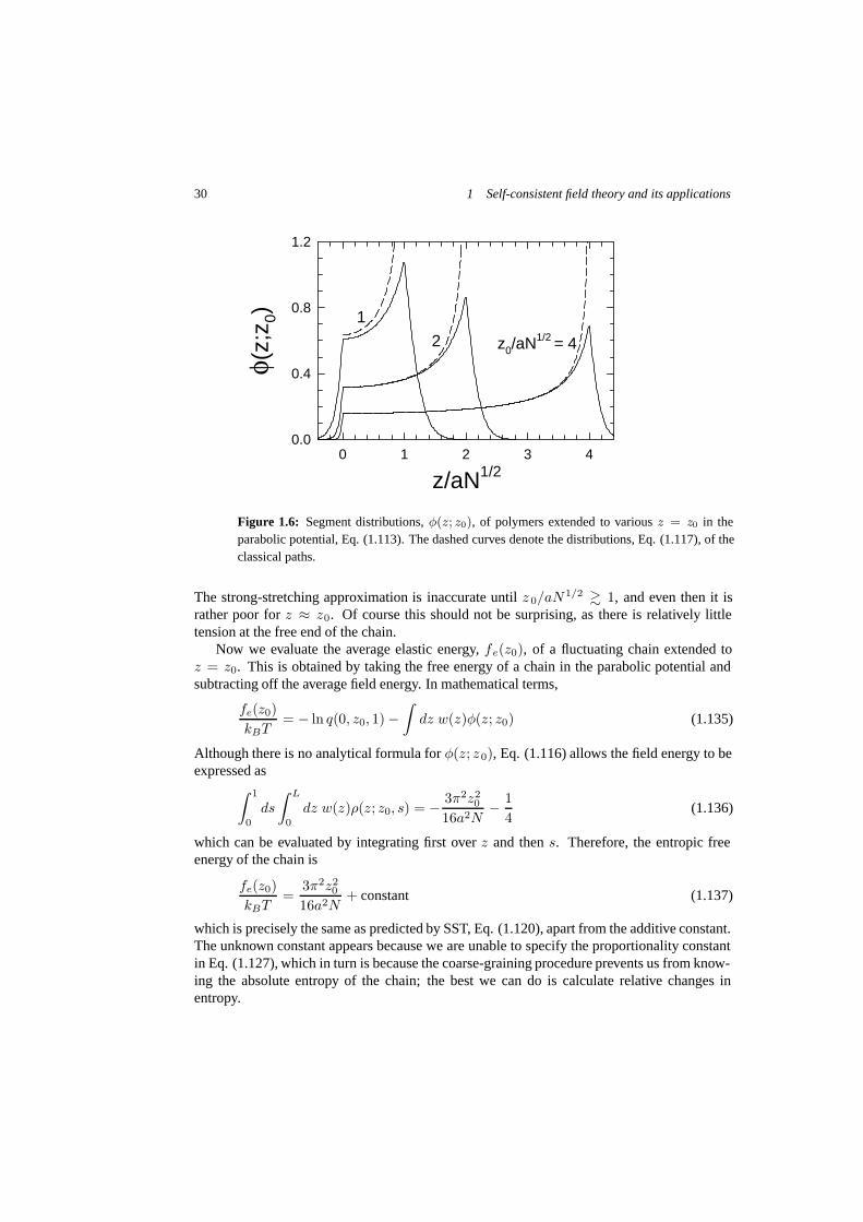
Figure 1.6: Segment distributions, φ(z; z0), of polymers extended to various z = z0 in theparabolic potential, Eq. (1.113). The dashed curves denote the distributions, Eq. (1.117), of theclassical paths.
The strong-stretching approximation is inaccurate until z 0/aN1/2 � 1, and even then it israther poor for z ≈ z0. Of course this should not be surprising, as there is relatively littletension at the free end of the chain.
Now we evaluate the average elastic energy, fe(z0), of a fluctuating chain extended toz = z0. This is obtained by taking the free energy of a chain in the parabolic potential andsubtracting off the average field energy. In mathematical terms,
fe(z0)kBT
= − ln q(0, z0, 1) −∫
dz w(z)φ(z; z0) (1.135)
Although there is no analytical formula for φ(z; z0), Eq. (1.116) allows the field energy to beexpressed as∫ 1
0
ds
∫ L
0
dz w(z)ρ(z; z0, s) = − 3π2z20
16a2N− 1
4(1.136)
which can be evaluated by integrating first over z and then s. Therefore, the entropic freeenergy of the chain is
fe(z0)kBT
=3π2z2
0
16a2N+ constant (1.137)
which is precisely the same as predicted by SST, Eq. (1.120), apart from the additive constant.The unknown constant appears because we are unable to specify the proportionality constantin Eq. (1.127), which in turn is because the coarse-graining procedure prevents us from know-ing the absolute entropy of the chain; the best we can do is calculate relative changes inentropy.

1.6 Polymer Brushes 31
1.6.3 Diffusion Equation for a Parabolic Potential
In Section 1.2, we established that the path-integral definition of the partition function is equiv-alent to the one based on the diffusion equation, just as Feynman’s path-integral formalism ofquantum mechanics coincides with Schrodinger’s differential equation. As in quantum me-chanics, the differential equation approach is generally the more practical method of calculat-ing q(z, z0, s). Here, we demonstrate that it indeed gives identical results to those obtained inthe previous section, where the path-integral approach was used.
Normally the diffusion Eq. (1.24) has to be solved numerically, but there already exists aknown analytical solution for parabolic potentials (Merzbacher 1970). In fact, it was originallyderived for the wavefunction of a simple harmonic oscillator; once again, we benefit from theanalogy with quantum mechanics. Transforming the quantum mechanical wavefunction inMerzbacher (1970), according to Eqs. (1.50)-(1.56) for the parabolic potential in Eq. (1.113),gives
q(z, z0, s) =(
34 sin(πs/2)
)1/2
exp(−3π[(z2 + z2
0) cos(πs/2) − 2zz0]4a2N sin(πs/2)
)(1.138)
Although the derivation of this expression is complicated, it is relatively trivial to confirm thatit is in fact the proper solution to Eq. (1.24) for the initial condition, q(z, z 0, 0) = aN1/2δ(z−z0).
Substituting z = 0 and s = 1 into Eq. (1.138), we find that q(0, z0, 1) =√
3/4, consis-tent with the path-integral calculation in Eq. (1.127). In terms of the partition function, thedistribution of the sN ’th segment is given by
ρ(z; z0; s) =q(0, z, 1 − s)q(z, z0, s)
q(0, z, 1)(1.139)
The derivation is essentially the same as that for Eq. (1.31). Inserting Eq. (1.138) and sim-plifying with some basic trigonometric identities gives the identical expression to that in Eq.(1.134), as required by the equivalence of the two approaches. Given this, the remaining re-sults of the preceding section follow. One slight difference is that we now obtain a specificvalue for the unknown constant in Eq. (1.137), because the initial condition for q(z, z 0, s),in effect, selects a proportionality constant for Eq. (1.127), but not one with any physicalsignificance. Nevertheless, this provides us with a standard reference by which to comparecalculations.
1.6.4 Self-Consistent Field Theory (SCFT) for a Brush
The parabolic potential used up to now is only approximate. The argument for it assumes thatthe tension at the free chain-end is zero, but there is in fact a small entropic force that acts tobroaden the end-segment distribution, g(z0) (Matsen 2002b). Here, the self-consistent fieldtheory (SCFT) is described for determining the field in a more rigorous manner. The theorystarts with the partition function for the entire system, which is written as
Z ∝∫ (
n∏α=1
Drαδ(zα(1) − ε)
)δ[1 − φ] (1.140)

32 1 Self-consistent field theory and its applications
where the tildes, Drα ≡ DrαP [rα], denote that the functional integrals are weighted by
P [rα] = exp(− 3
2a2N
∫ 1
0
ds|r′α(s)|2)
(1.141)
so as to account for the internal entropy of each coarse-grained segment. The functionalintegrals over each rα(s) are, in principle, restricted to the volume of the system, V = AL.To ensure that the chains are properly grafted to the substrate, there are Dirac delta functionsconstraining the s = 1 end of each chain to z = ε; we will eventually take the limit ε → 0.Furthermore, there is a Dirac delta functional that constrains the overall concentration, φ(r),to be uniform over all r ∈ V .
Although the expression for Z is inherently simple, its evaluation is far from trivial.Progress is made by first replacing the delta functional by the integral representation,
δ[1 − φ] ∝∫
DW exp(
ρ0
N
∫dr W (r)[1 − φ(r)]
)(1.142)
This expression is equivalent to Eq. (1.335) derived in the Appendix, but with k(x) substitutedby −iρ0W (r)/N . The constants, ρ0 and N , have no effect on the limits of integration, butthe i implies that W (r) must be integrated in the complex plane along the imaginary axis.Inserting Eq. (1.142) into Eq. (1.140) and substituting φ(r) by Eqs. (1.13) and (1.108)allows the integration over the chain trajectories to be performed. This results in the revisedexpression,
Z ∝∫
DW (Q[W ])n exp(
ρ0
N
∫dr W (r)
)(1.143)
where
Q[W ] ∝∫
Drα exp(−
∫ 1
0
ds W (rα(s)))
δ(zα(1) − ε) (1.144)
is the partition function of a single polymer in the external field, W (r). For convenience, thepartition function of the system is reexpressed as
Z ∝∫
DW exp(−F [W ]
kBT
)(1.145)
where
F [W ]nkBT
≡ − ln( Q[W ]AaN1/2
)− 1
V∫
dr W (r) (1.146)
There are a couple of subtle points that need to be mentioned. Firstly, the present cal-culation of Z allows the grafted ends to move freely in the z = ε plane, when actually theyare grafted to particular spots on the substrate. As long as the chains are densely grafted, theonly real consequence of treating the ends as a two-dimensional gas is that Q[W ] becomesproportional to A, the area available to each chain end. To correct for this, the Q[W ] in Eq.

1.6 Polymer Brushes 33
(1.146) is divided by A, which is necessary for F [W ] to be a proper extensive quantity thatscales with the size of the system. Alternatively, we could imagine that the chain ends arefree to move, but then the molecules would become indistinguishable and Z would have tobe divided by a factor of n! to avoid the Gibbs paradox (Reif 1965). Either way, we arriveat the same expression for F [W ] apart from additive constants. That bring us to the secondpoint that additive constants to F [W ] are of no consequence, since they can be absorbed intothe proportionality constant omitted in Eq. (1.145). This fact has been used to insert an extrafactor of aN 1/2 into Eq. (1.146) to make the argument of the logarithm dimensionless.
Even though W (r) takes on imaginary values, Q[W ] is solved by the exact same methodsderived in Section 1.2, and thus F [W ] is readily computed. However, the functional integralin Eq. (1.145) cannot be performed exactly. To proceed further, we use the fact that F [W ]is an analytic functional, which means that the path of integration can be deformed withoutaltering the integral. A standard trick to solve such integrals, the method of steepest descent(Carrier et al. 1966), is to deform the path from the imaginary axis to one that passes througha point where
DF [W ]DW (r)
= 0 (1.147)
in a direction such that the imaginary part of F [W ] remains constant. At such a point, the realpart of F [W ] has a saddle shape, and consequently it is denoted as a saddle point . Changingthe path of integration in this way concentrates the non-zero contribution of the integral to theneighborhood of the saddle point, allowing for a convenient expansion of which the first termgives
Z ≈ exp(−F [w]
kBT
)(1.148)
where w(r) is the solution to Eq. (1.147). Thus, F [w] becomes the SCFT approximation tothe free energy of the system. It follows from the functional differentiation in Eq. (1.147),that w(r) must be chosen such that
φ(r) = 1 (1.149)
where
φ(r) ≡ −VD ln(Q[w])Dw(r)
(1.150)
is the segment concentration of n polymers in the external field, w(r); see Eq. (1.32).
The quantity, φ(r), can also be identified as the SCFT approximation for⟨φ(r)
⟩, but the
explanation for this is often glossed over. It is justified by starting with the formal definition,
⟨φ(r)
⟩≡ 1
Z
∫ (n∏
α=1
Drαδ(zα(1) − ε)
)φ(r)δ[1 − φ] (1.151)

34 1 Self-consistent field theory and its applications
where here Z is evaluated with the missing proportionality constant set to one. Of course, the
Dirac delta functional implies that⟨φ(r)
⟩= 1, but let us instead evaluate it in the manner of
SCFT. With steps equivalent to those that lead to Eq. (1.145), we arrive at
⟨φ(r)
⟩=
1Z
∫DWφ(r) exp
(−F [W ]
kBT
)(1.152)
Here, φ(r) is the concentration of n polymers subjected to the fluctuating field, W (r), butsince the integrand is dominated by W (r) ≈ w(r), the concentration can be evaluated atthe saddle point. This allows φ(r) to be moved outside the functional integration, leadingimmediately to our intended identity,
⟨φ(r)
⟩≈ φ(r)
Z
∫DW exp
(−F [W ]
kBT
)= φ(r) (1.153)
With the saddle-point approximation, the calculation now becomes tractable. The partitionfunction for a chain in the field, w(z), with its s = 1 end fixed at z = ε is
Q[w]V =
1L
∫ L
0
dz q(z, s)q†(z, s) (1.154)
where the integral can be evaluated with any 0 ≤ s ≤ 1. The partial partition function,q(z, s), is obtained by solving the diffusion Eq. (1.24) with the initial condition, q(z, 0) = 1,and similarly the complementary function, q †(z, s), is calculated with Eq. (1.28), subject toq†(z, 1) = aN1/2δ(z − ε). These quantities also provide the concentration,
φ(z) =V
Q[w]
∫ 1
0
ds q(z, s)q†(z, s) (1.155)
which must be equated to one, by an appropriate adjustment of the field, w(z). Once the fieldis determined self-consistently, the free energy of the brush, F [w], can be evaluated using Eq.(1.146).
1.6.5 Boundary Conditions
In the bulk region of a melt, the long-range attractive interactions favoring a high densityare balanced against short-range hard-core interactions to produce a more or less uniformsegment concentration, ρ0. The details of this mechanism are easily avoided by invoking theincompressibility assumption, φ(r) = 1. This is no longer valid near the substrate (z = 0) northe air interface (z = L). At any surface, the dimensionless concentration, φ(r), must dropto zero. Although the decay in concentration is generally very sharp, it cannot occur as a truestep function. Instead, there must be a continuous surface profile, φ s(z), that switches from 1to 0 over a narrow region next to the surface.
The calculation of φs(z) requires an involved treatment that takes a detailed account ofthe molecular interactions. (Although we will be explicitly referring to the z = 0 surface,everything we say applies equally to the z = L surface.) In a proper treatment, the partial

1.6 Polymer Brushes 35
partition functions would be solved under the boundary conditions, q(0, s) = q †(0, s) = 0,which prevents the polymers from crossing the z = 0 plane and ensures that φ s(z) → 0 asz → 0. For discussion purposes, we will assume that the profile is not so sharp as to invalidateour coarse-grained model. It will certainly be sharp enough for the ground-state-dominanceapproximation to hold, which implies that the surface field is given by
ws(z) =a2N
6∇2
√φs(z)√
φs(z)(1.156)
However, one further relation between ws(z) and φs(z) is required in order to solve for thesurface profile. This is where the details of the molecular interactions must enter.
Provided that we are not concerned with knowing the details of the surface, such as φ s(z)and the resulting surface tension, it is possible to proceed without a full treatment of thesurface profile. This involves implementing the alternative boundary conditions,
∂
∂zq(0, s) =
∂
∂zq†(0, s) = 0 (1.157)
and solving the SCFT for w(z) ignoring the deviation from φ(z) = 1 at the surface. The fullsolution would only differ in the narrow region next to the substrate where φ s(z) < 1. Morespecifically, if we were given φs(z), the proper solution would be obtained by making thesubstitutions,
q(z, s) ⇒ q(z, s)√
φs(z) (1.158)
q†(z, s) ⇒ q†(z, s)√
φs(z) (1.159)
w(z) ⇒ w(z) + ws(z) (1.160)
The added factor of√
φs(z) would restore the proper boundary condition for the partial parti-tion functions, and would transform the concentration profile from φ(z) = 1 to φ(z) = φ s(z).One can also confirm that the transformation in the field is exactly as required for the trans-formed partition functions to satisfy the diffusion Eqs. (1.24) and (1.28); the proof of thisrequires that the pretransformed partition functions satisfy[
∂
∂zq(z, s)
] [∂
∂z
√φs(z)
]=
[∂
∂zq†(z, s)
] [∂
∂z
√φs(z)
]= 0 (1.161)
Indeed, it is safe to assume that the boundary conditions in Eq. (1.157) extend over the narrowregion where φs(z) has a nonzero gradient.
For most problems such as the brush, we simply assume that there is no variation in theprofile, φs(z), of each surface, rendering them as inert features that conveniently decouplefrom the behavior of the remaining system. Thus, we can continue to ignore the details of themolecular interactions and solve the field subject to the incompressibility condition, φ(z) = 1,with the partial partition functions satisfying reflecting boundary conditions, Eq. (1.157), atz = 0 and z = L.
For the case of the polymer brush, there is still one more issue to deal with at the z = 0substrate. The grafting of the chain ends in a perfect plane, which for the moment is at z = ε,produces a delta function in the field (Likhtman and Semenov 2000). Our intention is to

36 1 Self-consistent field theory and its applications
incorporate this singularity into the boundary condition, restoring w(z) to a continuous, finitefunction. We must, however, begin with the true field,
wt(z) =βa2N
6δ(z − ε) + w(z) (1.162)
containing the singularity at a small infinitesimal distance, ε, from the substrate. The diffusionEq. (1.24) requires the delta function in w t(z) to be balanced by an infinity in ∇2q(ε, s). Inother words, the delta function produces a sharp kink in ∂
∂z q(z, s) at z = ε, and similarly in∂∂z q†(z, s). The strength of the kink is determined by integrating the diffusion equation fromz = 0 to 2ε, which gives
a2N
6
[∂
∂zq(2ε, s) − ∂
∂zq(0, s)
]− βa2N
6q(ε, s) ≈ 0 (1.163)
Our original reflecting boundary condition implies that ∂∂z qz(0, s) = 0. Dropping this term
from Eq. (1.163) and then taking the limit ε → 0 yields the new boundary condition,
∂
∂zq(0, s) = βq(0, s) (1.164)
Naturally, the complementary partition function, q †(z, s), satisfies the same boundary condi-tion at z = 0. The constant β is determined by the requirement that w(z) does not develop adelta function at z = 0.
1.6.6 Spectral Solution to SCFT
There are two main ways to solve the SCFT; one is a direct real-space method (Matsen 2004),where the diffusion equations are solved using finite differences for the derivatives (the Crank-Nicolson algorithm), and the other involves a spectral method (Matsen and Schick 1994a)much like that discussed in Section 1.5.1. The spectral method is particularly efficient forlower grafting densities, while the real-space one is better suited to thick brushes. Note thatthere are also semi-spectral algorithms (Rasmussen and Kalosakas 2002) that combine theadvantages of the two methods. Here, we demonstrate the spectral method.
Since the field is unknown, the functional expansions will be performed in terms of Lapla-cian eigenfunctions, fi(z), defined by
∇2fi(z) = − λi
L2fi(z) (1.165)
subject to the boundary conditions, f ′i(0) = βfi(0) and f ′
i(L) = 0. Note that the L2 in Eq.(1.165) has been included so that λi becomes dimensionless. The solution to this eigenvalueproblem is
fi(z) = Ci cos(√
λi(1 − z/L))
(1.166)
where the boundary conditions require√λi tan
(√λi
)= βL (1.167)

1.6 Polymer Brushes 37
With the normalization constant set to
Ci =
√4√
λi
2√
λi + sin(2√
λi
) (1.168)
the basis functions obey the orthonormal condition in Eq. (1.60). Once the basis functionsare determined, there are a couple of useful quantities to calculate. The first is the symmetrictensor,
Γijk ≡ 1L
∫dzfi(z)fj(z)fk(z) (1.169)
and the second is the set of coefficients for the identity function,
Ii ≡ 1L
∫ L
0
dzfi(z) = Ci
sin(√
λi
)√
λi
(1.170)
defined such that∑
i Iifi(z) = 1.With the preamble complete, we are now ready to solve for the partial partition function.
The procedure is slightly more involved than in Section 1.5.1, because the field is now omittedfrom Eq. (1.165), but that is the price we pay to have simple basis functions. Nevertheless,the procedure is much the same. The expansions, q(z, s) =
∑i qi(s)fi(z) and w(z) =∑
k wkfk(z), are first inserted into the diffusion Eq. (1.24), giving
∑i
dqi(s)ds
fi(z) = −a2N
6L2
∑i
λiqi(s)fi(z) −∑ik
wkqi(s)fi(z)fk(z) (1.171)
By multiplying through by fj(z), integrating over r, and using the orthonormal condition, thiscan be rewritten as a system of first-order linear ordinary differential equations,
d
dsqi(s) =
∑j
Aijqj(s) (1.172)
subject to the initial conditions, qi(0) = Ii. The coefficients of the matrix, A, are given by
Aij ≡ −λia2N
6L2δij −
∑k
wkΓijk (1.173)
Note that the boundary conditions on q(z, s) are already accounted for by those on f i(z).The solution to Eq. (1.172) is simply
qi(s) =∑
j
Tij(s)qj(0) (1.174)
where T(s) ≡ exp(As) is referred to as a transfer matrix. To evaluate it, we perform a matrixdiagonalization
A = UDU−1 (1.175)

38 1 Self-consistent field theory and its applications
where the elements of the diagonal matrix, dk ≡ Dkk , are the eigenvalues of A and the re-spective columns of U are the corresponding normalized eigenvectors. Since A is symmetric,all the eigenvalues will be real and U−1 = UT . We can then express T(s) = U exp(Ds)UT ,from which it follows that
Tij(s) =∑
k
exp(sdk)UikUjk (1.176)
Similarly, the solution for the complementary function, q †(z, s) ≡ ∑i q†i (s)fi(z), is given by
q†i (s) =∑
j
Tij(1 − s)q†j(1) (1.177)
where
q†i (1) =1L
∫ L
0
dzq†(z, 1)fi(z) = Ci cos(√
λi
) aN1/2
L(1.178)
This result is obtained by first integrating with q†(z, 1) = aN1/2δ(z − ε), and then taking thelimit, ε → 0. Once the partial partition functions are evaluated, the partition function for theentire chain is obtained by
Q[w]V =
∑i
qi(s)q†i (s) =
∑i
exp(di)qi(0)q†i (1) (1.179)
where we have made the convenient definitions, q i(0) ≡ ∑j qj(0)Uji and q†i (1) ≡ ∑
j q†j (1)Uji.
z/L0.0 0.2 0.4 0.6 0.8 1.0
w(z
) a2 N
/L2
-3
-2
-1
0
1
2
24
L/aN1/2 = 1
Figure 1.7: Self-consistent field, w(z), plotted for several brush thicknesses, L. The dashedcurve denotes the SST prediction in Eq. (1.113), shifted vertically such that its average is zero.

1.6 Polymer Brushes 39
The coefficients of the average polymer concentration can be expressed as
φi =V
Q[w]
∑jk
IjkΓijk (1.180)
where the components of the matrix, I, are defined as
Ijk ≡∫ 1
0
ds qj(s)q†k(s) (1.181)
=∑m,n
[exp(dm) − exp(dn)
dm − dn
]UjmUknqm(0)q†n(1) (1.182)
Note that in the instances where dm = dn, the factor in the square brackets reduces toexp(dm).
Given the formula to evaluate the segment concentration, the coefficients of the field, w i,can now be adjusted to satisfy the incompressibility condition, φ(z) = 1, which is expressedin terms of coefficients as
φi = Ii (1.183)
In practice, the functional expansion has to be truncated at some value i = M , where M ischosen based on an acceptable error tolerance. In principle, the first (M +1) components, w i,would be adjusted to satisfy the first (M +1) conditions for φ i. However, Eqs. (1.183) are notcompletely independent, due to the fact that SCFT is not affected by an additive constant tow(z); see the discussion at the end of Section 1.2. To rectify this problem, the first condition,φ0 = I0, can be replaced by∑
i
Iiwi = 0 (1.184)
which sets the spatial average of w(z) to zero. Now the set of equations are independent,and they can be solved by standard numerical techniques. There are various techniques thatcan be used (Thompson et al. 2004); we generally use the Broyden algorithm, which is aquasi-Newton-Raphson method. This requires a reasonable initial guess for w(z), but that canbe provided by the SST estimate in Eq. (1.113). Figure 1.7 shows the field, w(z), obtainedfrom SCFT (solid curves) for several different brush thicknesses compared against the SSTresult (dashed curve) from Eq. (1.113). As expected, the SST prediction becomes increasinglyaccurate as L → ∞.
We have glossed over the fact that β was introduced in order to prevent a delta functionfrom developing in w(z) at z = 0. The signature of a delta function is that the field coeffi-cients, wi, fail to converge to zero in the limit of large i. To prevent this, we could include theextra condition, wM = 0, in our Broyden iterations and use it to determine β. The estimate,β ≈ 3L/a2N , by Likhtman and Semenov (2000) provides a suitable initial guess. In reality,this initial guess turns out to be very accurate, and since the spectral method can cope witha small delta function, we simply use the initial guess provided by Likhtman and Semenov(2000).

40 1 Self-consistent field theory and its applications
z0/L0.0 0.2 0.4 0.6 0.8 1.0
g(z 0)
L/a
N1/
2
0
1
2
3
4
2
4
L/aN1/2 = 1
Figure 1.8: End-segment distribution, g0(z0), calculated by SCFT for several brush thicknesses,L. The dashed curve denotes the SST prediction from Eq. (1.119).
Although the end-segment distribution function, g(z 0), is not a direct by-product of SCFT,it is easily evaluated. The formula for it,
g(z0) =V
Q[w]q†(z0, 0) (1.185)
is derived in the same manner as Eq. (1.155) for φ(z). Figure 1.8 shows the SCFT predictionfor g(z0) (solid curves) calculated for several different brush thicknesses compared against theSST prediction (dashed curve) from Eq. (1.119). As with the field, SST becomes increasinglyaccurate as L → ∞.
The free energy of the brush is given by
F
nkBT= − ln
( Q[w]AaN1/2
)− βa2N
6L(1.186)
The second term comes from the delta function contribution to the true potential, w t(z), in Eq.(1.162), which was removed from w(z) by the use of the boundary condition in Eq. (1.164).The resulting energy is plotted in Fig. 1.9. Included with a dotted curve is an approximation,
F
nkBT≈ π2L2
8a2N−ln
( √3L
2aN1/2
)+0.1544−0.64
(L
aN1/2
)−2/3
−0.09(
L
aN1/2
)−4/3
(1.187)
based on a theoretical expansion by Likhtman and Semenov (2000). The two coefficients of0.64 and 0.09 were obtained by a previous fit to SCFT (Matsen 2004) at L/aN 1/2 � 1, butas Fig. 1.9 clearly shows, the fit remains accurate down to reasonably low values of L. Noticethat the dominant term in Eq. (1.187) is precisely the SST prediction from Eq. (1.121).
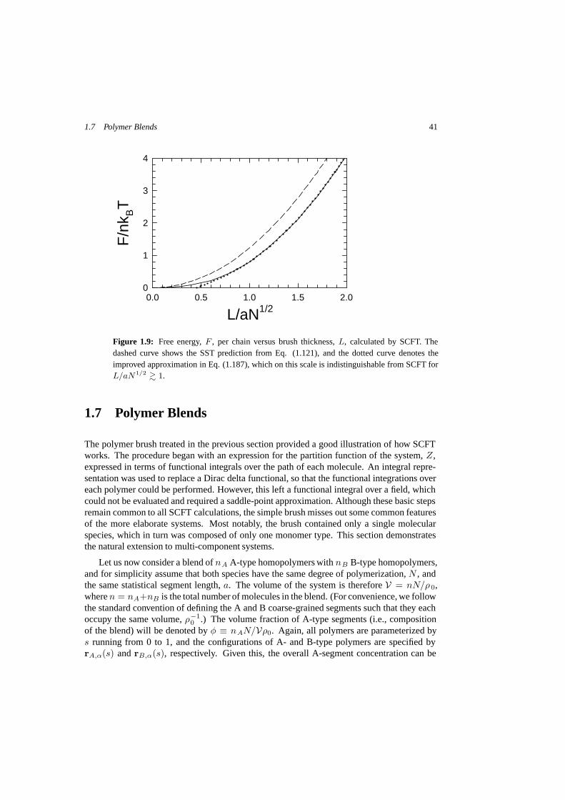
1.7 Polymer Blends 41
L/aN1/20.0 0.5 1.0 1.5 2.0
F/n
k BT
0
1
2
3
4
Figure 1.9: Free energy, F , per chain versus brush thickness, L, calculated by SCFT. Thedashed curve shows the SST prediction from Eq. (1.121), and the dotted curve denotes theimproved approximation in Eq. (1.187), which on this scale is indistinguishable from SCFT forL/aN1/2 � 1.
1.7 Polymer Blends
The polymer brush treated in the previous section provided a good illustration of how SCFTworks. The procedure began with an expression for the partition function of the system, Z ,expressed in terms of functional integrals over the path of each molecule. An integral repre-sentation was used to replace a Dirac delta functional, so that the functional integrations overeach polymer could be performed. However, this left a functional integral over a field, whichcould not be evaluated and required a saddle-point approximation. Although these basic stepsremain common to all SCFT calculations, the simple brush misses out some common featuresof the more elaborate systems. Most notably, the brush contained only a single molecularspecies, which in turn was composed of only one monomer type. This section demonstratesthe natural extension to multi-component systems.
Let us now consider a blend of nA A-type homopolymers with nB B-type homopolymers,and for simplicity assume that both species have the same degree of polymerization, N , andthe same statistical segment length, a. The volume of the system is therefore V = nN/ρ 0,where n = nA+nB is the total number of molecules in the blend. (For convenience, we followthe standard convention of defining the A and B coarse-grained segments such that they eachoccupy the same volume, ρ−1
0 .) The volume fraction of A-type segments (i.e., compositionof the blend) will be denoted by φ ≡ nAN/Vρ0. Again, all polymers are parameterized bys running from 0 to 1, and the configurations of A- and B-type polymers are specified byrA,α(s) and rB,α(s), respectively. Given this, the overall A-segment concentration can be

42 1 Self-consistent field theory and its applications
expressed as
φA(r) =N
ρ0
nA∑α=1
∫ 1
0
ds δ(r − rA,α(s)) (1.188)
with an analogous expression specifying the B-segment concentration, φB(r).With the inclusion of two chemically distinct segments, it is no longer possible to side-
step the issue of monomer-monomer interactions. For discussion purposes, assume that theinteraction between two monomers, i and j, obeys a simple Lennard-Jones potential,
u(rij) = ε
[(σ
rij
)12
− 2(
σ
rij
)6]
(1.189)
where rij is their separation. The incompressibility assumption
φA(r) + φB(r) = 1 (1.190)
acts to maintain the spacing between neighboring monomers at the minimum of the potentialenergy, rij = σ. The detailed shape of the potential is therefore no longer needed; we cansimply assume that the interaction energy is −ε between neighboring monomers and zerootherwise. In the brush system, all the interactions were the same and thus they added upto a constant energy that could be ignored, assuming the total number of monomer contactsremained more or less fixed. In the blend, however, we must account for the fact that thedepth of the potential will differ between the A-A, A-B, and B-B contacts. Noting that therange of the monomer-monomer interactions, σ, is negligible on the coarse-grained scale, theinteractions can be treated as contact energies and thus the internal energy can be expressedas
U ≡ −N2εAA
2ρ20
∑α,β
∫ds dt δ(rA,α(s) − rA,β(t)) −
N2εAB
ρ20
∑α,β
∫ds dt δ(rA,α(s) − rB,β(t)) −
N2εBB
2ρ20
∑α,β
∫ds dt δ(rB,α(s) − rB,β(t)) (1.191)
Using the incompressibility assumption, φA(r) + φB(r) = 1, this simplifies to
U [φA, φB ]kBT
= χρ0
∫dr φA(r)φB(r) (1.192)
where the interaction strengths are grouped together into a single dimensionless parameter,
χ ≡ εAA − 2εAB + εBB
2kBTρ0(1.193)

1.7 Polymer Blends 43
Note that the value of χ is inversely proportional to the segment density, ρ 0, and thus is notan invariant quantity; one must be careful of this fact when referring to literature values of χ.Equation (1.192) is the simplest and by far most common expression for the interactions, butSCFT is perfectly capable of accommodating more elaborate treatments (Matsen 2002a), if sodesired.
1.7.1 SCFT for a Polymer Blend
The partition function for a polymer blend is hardly any more involved than that for the poly-mer brush in Section 1.6.4. In this case, it becomes
Z ∝ 1nA!nB!
∫ nA∏α=1
DrA,α
nB∏β=1
DrB,β exp
(−U [φA, φB]
kBT
)δ[1− φA − φB] (1.194)
As before, there is a functional integration over the configuration of each polymer and a Diracdelta functional is used to enforce the incompressibility condition. Of course, the delta func-tions constraining the chain ends are gone, and there is now a Boltzmann weight accountingfor the energy of the segment interactions. Also present are factors of n A! and nB! to accountfor the indistinguishability of the A- and B-polymers, respectively.
This time, we start by inserting a functional integral over δ[ΦA − φA], allowing the opera-tor, φA(r), to be swapped with the ordinary function, ΦA(r). This transforms δ[1− φA − φB]into δ[1−ΦA− φB], which, in turn, allows the exchange of φB(r) with 1−ΦA(r). The resultof this manipulation is
Z ∝ 1nA!nB!
∫DΦA
nA∏α=1
DrA,α
nB∏β=1
DrB,β exp(−U [ΦA, 1 − ΦA]
kBT
)×
δ[ΦA − φA]δ[1 − ΦA − φB ] (1.195)
As with the brush, the two delta functionals are replaced with integral representations anal-ogous to that in Eq. (1.142), which allows us to complete the integrals over the polymerconfigurations, leading to the result,
Z ∝ 1nA!nB!
∫DΦADWADWB
(ρ0
NQA[WA]
)nA(ρ0
NQB[WB]
)nB ×
exp(−U [ΦA, 1 − ΦA]
kBT+
ρ0
N
∫dr[WAΦA + WB(1 − ΦA)]
)(1.196)
where
Qγ [Wγ ] ∝∫
Drγ,α exp(−
∫ 1
0
ds Wγ(rγ,α(s)))
(1.197)
is the partition function of a single γ-type polymer in the external field, W γ(r). (For thepurpose of future simplification, a factor of (ρ0/N)n has been extracted from the unspecifiedproportionality constant in Eq. (1.196).) Next, the factorials are replaced by the usual Stirlingapproximations (e.g., ln(nγ !) ≈ nγ ln(nγ) − nγ), giving
Z ∝∫
DΦADWADWB exp(−F [ΦA, WA, WB ]
kBT
)(1.198)

44 1 Self-consistent field theory and its applications
where
F
nkBT= φ
[ln
(φV
QA[WA]
)− 1
]+ (1 − φ)
[ln
((1 − φ)VQB[WB ]
)− 1
]+
1V
∫dr[χNΦA(1 − ΦA) − WAΦA − WB(1 − ΦA)] (1.199)
As before with the brush, all the steps above are exact. The partition functions, QA[WA]andQB[WB ], can still be calculated by the method outlined in Section 1.2, and thus F [Φ A, WA, WB]can be evaluated without difficulty. It is the functional integration of exp(−F/k BT ) in Eq.(1.198) that poses a problem. So once again, the saddle-point approximation is implemented,which requires us to locate the extremum denoted by the lower-case functions, φ A, wA, andwB . Setting to zero the functional derivative of F [ΦA, WA, WB ] with respect to WA gives thecondition,
φA(r) = −VφD ln(QA[wA])
DwA(r)(1.200)
Equation (1.32) identifies φA(r) as the average concentration of nA polymers in the externalfield, wA(r), which is evaluated by
φA(r) = − Vφ
QA[wA]
∫ 1
0
ds qA(r, s)q†A(r, s) (1.201)
where
QA[wA] =∫
dr qA(r, s)q†A(r, s) (1.202)
Here, the partial partition functions, qA(r, s) and q†A(r, s), obey the previous diffusion Eqs.(1.24) and (1.28), but with the field, wA(r). Differentiation of F [ΦA, WA, WB ] with respectto WB leads to the incompressibility requirement,
φA(r) + φB(r) = 1 (1.203)
where
φB(r) ≡ −VφD ln(QB[wB ])
DwB(r)(1.204)
is the average concentration of nB polymers in the external field, wB(r), evaluated in the samemanner as φA(r). Following arguments already presented in Section 1.6.4, φA(r) and φB(r)are the SCFT approximations for
⟨φA(r)
⟩and
⟨φB(r)
⟩, respectively. The last remaining
differentiation of F [ΦA, WA, WB] with respect to ΦA gives the self-consistent field condition,
wA(r) − wB(r) = χN(1 − 2φA(r)) (1.205)
In principle, the two Eqs. (1.203) and (1.205) should be enough to determine the twofunctions, wA(r) and wB(r), but this is not exactly the case. With similar arguments to those

1.7 Polymer Blends 45
at the end of Section 1.2, one can show that F [φA, wA, wB ] is unaffected by an added constantto either wA(r) or wB(r). These degrees of freedom can be removed by fixing their spatialaverages to wA = wB = 0, and adding an appropriate constant to Eq. (1.205) such that
wA(r) − wB(r) = 2χN(φ − φA(r)) (1.206)
With this revised field equation, the SCFT approximation of the free energy, F [φ A, wA, wB],given by Eq. (1.199) can be reexpressed as
F
nkBT=
Fh
nkBT− φ ln
(QA[wA]V
)− (1 − φ) ln
(QB[wB ]V
)−
χN
V∫
dr(φA(r) − φ)(φB(r) − 1 + φ) (1.207)
where
Fh
nkBT= φ[ln φ − 1] + (1 − φ)[ln(1 − φ) − 1] + χNφ(1 − φ) (1.208)
1.7.2 Homogeneous Phases and Macrophase Separation
The simplest solution to the self-consistent field equations is that for uniform fields, wA(r) =wB(r) = 0, corresponding to a homogeneous mixture. In this case, the partition functionsreduce to QA[wA] = QB[wB ] = V , and the segment concentrations simplify to φA(r) = φand φB(r) = 1−φ. Inserting these results into Eq. (1.207), we find that F = Fh. Indeed, Eq.(1.208) is the well-known Flory-Huggins expression for the free energy of a homogeneousblend of composition, φ. Figure 1.10(a) shows the free energy curve for χN = 3. Notice thatthere is a region, between the two inflection points denoted by diamond symbols, where thefree energy has negative curvature. This property implies that the system is unstable towardsmacrophase separation, where the melt splits into A- and B-rich phases occupying separateregions of the volume, V .
To determine whether or not the blend will macrophase separate, we need an expressionfor the combined energy free, Fs = F
(1)h + F
(2)h , of two distinct phases of compositions,
φ(1) and φ(2), respectively. If the blend is to macrophase separate, it has to obey some basicconservation rules. First, the number of molecules in the two phases, n (1) and n(2), mustsatisfy
n(1) + n(2) = n (1.209)
and second, the number of A-type polymers in each phase must comply with
n(1)φ(1) + n(2)φ(2) = nφ (1.210)
These conservation laws imply that the fraction of molecules in phase (1) will be
n(1)
n=
φ(2) − φ
φ(2) − φ(1)(1.211)

46 1 Self-consistent field theory and its applications
Now we can rewrite the total energy, Fs, of a macrophase separated system as
Fs
nkBT=
F(2)h
n(2)kBT+
(F
(1)h
n(1)kBT− F
(2)h
n(2)kBT
)n(1)
n(1.212)
which is plotted in Fig. 1.10(a) for the example where φ (1) = 0.3 and φ(2) = 0.6. It is clearfrom the form of Eqs. (1.211) and (1.212) that F s versus φ is simply a straight line extendingfrom Fs = F
(1)h and φ = φ(1) to Fs = F
(2)h and φ = φ(2). Naturally, the line must terminate
at φ(1) and φ(2) since the overall composition, φ, is a volume-average over two individualphases (i.e., φ(1) ≤ φ ≤ φ(2)). In this particular example, the entire line, Fs, lies below thecurve, Fh, and thus macrophase separation is preferred at all compositions, 0.3 < φ < 0.6.The volumes occupied by the two resulting phases would occur in the ratio,
n(1)
n(2)=
φ(2) − φ
φ − φ(1)(1.213)
which is known as the lever rule, on account of its graphical interpretation in terms of the twoportions, (φ(2)−φ) and (φ−φ(1)), of the straight line. Of course, the particular compositions,φ(1) = 0.3 and φ(2) = 0.6, do not represent the global free energy minimum.
The lowest possible energy that can be achieved by macrophase separation is determinedby the double-tangent construction denoted with a dotted line in Fig. 1.10(a). At any φ alongthis line, the blend will ultimately macrophase separate into the compositions at the two endsof the line marked by solid triangles and referred to as binodal points. Near these binodalcompositions, however, the system is metastable against macrophase separation and can existin the single mixed state for a considerable time. This is because the positive curvature in F h
causes the free energy to initially increase as φ(1) and φ(2) depart from the average compo-sition, φ. Only when φ(1) and φ(2) are sufficiently far apart does the system benefit from areduction in free energy. The presence of this energy barrier requires the phase separation toproceed by the slow process of nucleation and growth. In contrast, there is no energy barrierat compositions between the spinodal points denoted by the solid diamonds, due to the factthat the curvature in the free energy is negative. In this instance, phase separation is relativelyfast and occurs by a process referred to as spinodal decomposition.
In this symmetric case where both polymers are the same size, the double-tangent line ishorizontal and thus the binodals occur at zero slope in the free energy, which works out to be
χN =1
2φ − 1ln
(φ
1 − φ
)(1.214)
The spinodals occur when the second derivative is zero, which corresponds to
χN =1
2φ(1 − φ)(1.215)
The phase diagram in Fig. 1.10(b) shows the binodals (solid curves) between which the systemfavors macrophase separation, and the spinodals (dotted curves) between which the separationis more or less immediate. Both sets of curves terminate at a critical point (χN = 2), belowwhich the interaction strength is too weak to induce phase separation, regardless of the com-position.

1.7 Polymer Blends 47
φ0.0 0.2 0.4 0.6 0.8 1.0
χN
1
2
3
4
5
Fh/
nkBT
-1.08
-1.04
-1.00
-0.96
-0.92
(a) χN = 3
(b)
φ(1)
φ(2)
2-phase
1-phase
Fs
Figure 1.10: (a) Free energy, Fh, of a homogeneous blend as a function of composition, φ,calculated for χN = 3. The dashed line denotes the free energy, Fs, for a macrophase-separatedblend with compositions, φ(1) = 0.3 and φ(2) = 0.6, and the dotted line is the double-tangentconstruction locating the binodal points denoted by triangles. The two diamonds denote spinodalpoints, where the curvature of the free energy curve switches sign. (b) Phase diagram showingthe binodal (solid) and spinodal (dotted) curves as a function of χN . The triangular and diamondsymbols correspond to those in (a), and the solid dot denotes a critical point.
1.7.3 Scattering Function for a Homogeneous Blend
A beam of radiation (e.g., x-rays or neutrons) will pass undeflected through a perfectly homo-geneous blend, φA(r) = φ, assuming the wavelength, λ, is above the atomic resolution andthat absorption is negligible. However, there are always thermal functuations that disturb theuniform composition, which in turn scatter the radiation by various angles, θ. To predict the

48 1 Self-consistent field theory and its applications
resulting pattern of radiation, I(θ), we must first calculate the free energy cost, F [ΦA], of pro-ducing a specified composition fluctuation, φA(r) = ΦA(r). The fact that we will continue toimplement mean-field theory implies that, in reality, the free energy we calculate will be for a
fixed φA(r) ≡⟨φA(r)
⟩as opposed to a fixed φA(r); this limitation will be discussed further
in Section 1.10.
kaN1/20 1 2 3
S(k
)/N
0
1
2
3
1.5
φ = 0.5
χN=1.8
1.0
Figure 1.11: Scattering function, S(k), for binary blends of symmetric composition, φ = 0.5,plotted for several degrees of segregation, χN .
To perform the calculation, we use the Fourier representation developed in Section 1.5.4.In terms of the Fourier transforms of the composition, φA(k) and φB(k), the free energy isapproximated by
F
nkBT=
Fh
nkBT+
12φ(2π)3V
∫k �=0
dkφA(−k)φA(k)
g(x, 1)+
12(1 − φ)(2π)3V
∫k �=0
dkφB(−k)φB(k)
g(x, 1)+
χN
(2π)3V∫k �=0
dkφA(−k)φB(k) (1.216)
The first term is the free energy of a perfectly homogeneous state, Eq. (1.208), the followingtwo integrals represent the loss in configurational entropy, Eq. (1.105), experienced by the A-and B-type polymers, and the final integral accounts for the increased number of A-B contacts,Eq. (1.192) transformed by Eq. (1.82). The incompressibility condition is enforced by setting,φB(k) = −φA(k), which simplifies the free energy to
F
nkBT=
Fh
nkBT+
N
2(2π)3V∫k �=0
dkS−1(k)φA(−k)φA(k) (1.217)
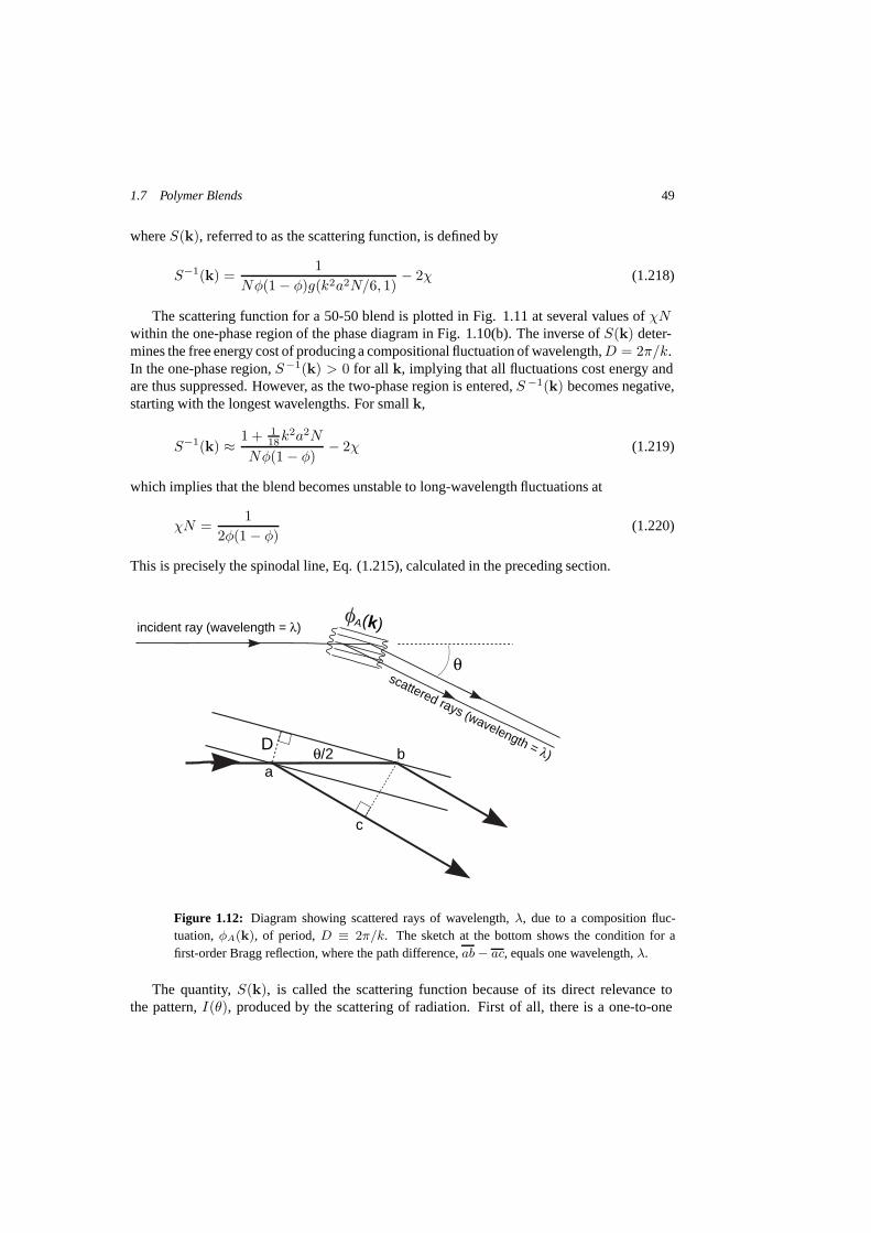
1.7 Polymer Blends 49
where S(k), referred to as the scattering function, is defined by
S−1(k) =1
Nφ(1 − φ)g(k2a2N/6, 1)− 2χ (1.218)
The scattering function for a 50-50 blend is plotted in Fig. 1.11 at several values of χNwithin the one-phase region of the phase diagram in Fig. 1.10(b). The inverse of S(k) deter-mines the free energy cost of producing a compositional fluctuation of wavelength, D = 2π/k.In the one-phase region, S−1(k) > 0 for all k, implying that all fluctuations cost energy andare thus suppressed. However, as the two-phase region is entered, S −1(k) becomes negative,starting with the longest wavelengths. For small k,
S−1(k) ≈ 1 + 118k2a2N
Nφ(1 − φ)− 2χ (1.219)
which implies that the blend becomes unstable to long-wavelength fluctuations at
χN =1
2φ(1 − φ)(1.220)
This is precisely the spinodal line, Eq. (1.215), calculated in the preceding section.
incident ray (wavelength = λ)
scattered rays (wavelength = λ)
A(k)
θ
ab
c
θ/2D
Figure 1.12: Diagram showing scattered rays of wavelength, λ, due to a composition fluc-tuation, φA(k), of period, D ≡ 2π/k. The sketch at the bottom shows the condition for afirst-order Bragg reflection, where the path difference, ab − ac, equals one wavelength, λ.
The quantity, S(k), is called the scattering function because of its direct relevance tothe pattern, I(θ), produced by the scattering of radiation. First of all, there is a one-to-one

50 1 Self-consistent field theory and its applications
correspondence between k and θ due to the fact that a periodic compositional fluctuation ofwavevector, k, predominantly scatters radiation by a particular angle, θ, determined by theBragg condition outlined in Fig. 1.12. First-order constructive interference requires that thepath difference, ab − ac, equals one wavelength, λ, of the incident radiation. By simpletrigonometry, the path-length between points a and b is ab = D/ sin(θ/2), where D = 2π/kis the period of the composition fluctuation. The alternative path-length between a and c isac = ab cos(θ) = ab[1 − 2 sin2(θ/2)]. Thus, the Bragg condition relating k and θ is
θ = 2 sin−1
(λk
4π
)(1.221)
Second of all, the intensity of the scattered radiation, I(θ), is proportional to the ensemble av-erage of |φA(k)|2, where the orientation of k fulfils the Bragg condition. Since the probabilityof a harmonic fluctuation is given by the Boltzmann factor, exp(−cS −1(k)|φA(k)|2), wherec is independent of k and φA(k), it follows that
⟨|φA(k)|2⟩ ∝ S(k). This, in turn, impliesI(θ) ∝ S(k), and hence the name, scattering function.
1.7.4 SCFT for a Homopolymer Interface
When a blend macrophase separates, there is inevitably an interface between the two phasesas illustrated in Fig 1.3(b). Here, we calculate its properties and determine the resulting excessfree energy per area, referred to as the interfacial tension, γ I . Since the interface is unfavor-able, it tends to be flat so as to minimize its total area, A. Therefore, we set up a Cartesiancoordinate system with the z axis perpendicular to the interface, and we consider a volume,V = LA, where L is sufficiently large that the system attains the properties of the bulk A- andB-rich phases at z = −L/2 and z = L/2, respectively. Because of the translational symmetryparallel to the interface, there will be no spatial variation in the x and y directions. These factsallow us to impose reflecting boundary conditions at the edges of V .
As for the brush in Section 1.6.6, we again solve this problem using the spectral method.For the symmetry of our current problem, the appropriate basis functions are
fi(z) ={
1 , if i = 0√2 cos(iπ(1 + 2z/L)) , if i > 0
(1.222)
This is, in fact, the same set of functions used for the polymer brush in Eq. (1.166), but withβ = 0. In this case, the eigenvalues of the Laplacian become
λi = 4π2i2 (1.223)
and the symmetric tensor simplifies to
Γijk = (δi+j,k + δ|i−j|,k)/√
2 (1.224)
when all the indices are nonzero. If one or more of the indices are zero, then it reduces to asingle delta function (e.g. Γij0 = δij when k = 0).
The SCFT calculation for this system proceeds remarkably like that of the polymer brush,with only a couple of key differences. The first difference occurs because there are now two

1.7 Polymer Blends 51
distinct fields, wA(z) and wB(z), acting on the A and B segments, respectively. This resultsin two different transfer matrices, TA(s) ≡ exp(As) and TB(s) ≡ exp(Bs), where thecoefficients of A and B are
Aij ≡ −2π2i2a2N
3L2δij −
wA,(i+j) + wA,|i−j|√2
(1.225)
Bij ≡ −2π2i2a2N
3L2δij −
wB,(i+j) + wB,|i−j|√2
(1.226)
These matrices are equivalent to that in Eq. (1.173), but with the simplified expressions forλi and Γijk explicitly inserted. We have also assumed that the spatial averages of wA(z) andwB(z) are both zero, which, for the current set of basis functions, implies wA,0 = wB,0 = 0.
The fact that all chain ends are now free is accounted for by the conditions, q γ(r, 0) = 1and q†γ(r, 1) = 1, where γ denotes either an A- or B-type polymer. In terms of the coefficients,
qγ,i(s) and q†γ,i(s), these conditions become
qγ,i(0) = δi0 (1.227)
q†γ,i(1) = δi0 (1.228)
Other than this one minor difference, the calculation of the concentrations coefficients, φ γ,i,proceeds exactly as before in Eqs. (1.180) and (1.181).
The procedure for solving the self-consistent field Eqs. (1.203) and (1.206) changes everso slightly from the case of the polymeric brush. The summations are still truncated at i = M ,where M is large enough that the resulting inaccuracy is negligible. This time, however, thereis no β to worry about, and the arbitrary constant to the fields have already been taken careof by setting wA,0 = wB,0 = 0. The remaining 2M field coefficients are determined byrequiring
φA,i + φB,i = 0 (1.229)
wA,i − wB,i = −2χNφA,i (1.230)
for i = 1, 2, 3, ..., M . Once these equations are satisfied, the free energy is given by Eq.(1.207), which simplifies to
F
nkBT=
Fh
nkBT− φ ln(qA,0(1)) − (1 − φ) ln(qB,0(1)) − χN
M∑i=1
φA,iφB,i (1.231)
This expression is arrived at by the fact that Qγ = Vqγ,0(1), φA,0 = φ, and φB,0 = 1 − φ.Figure 1.13(a) shows the segment profiles calculated at several degrees of segregation
within the two-phase region of Fig. 1.10(b). The interface appears in the center of the systemat z = 0, because a symmetric blend composition of φ = 0.5 was chosen. A convenientdefinition for the width over which the profile switches between the A- and B-rich phases is
wI ≡ φA(L/2)− φA(−L/2)φ′
A(0)(1.232)
As χN increases, the interface becomes narrower as illustrated in Fig. 1.13(b) so as to reducethe overlap between the A- and B-segment profiles. The interfacial tension, γ I , associated

52 1 Self-consistent field theory and its applications
χN10 100
wI/a
N1/
2
0.1
1
z/aN1/2-1.6 -0.8 0.0 0.8 1.6
φA(z)
0.0
0.4
0.8
1.2
(a)
(b)
χN = 104
2.5
0.7
0.07
0.2
0.4
3 30
Figure 1.13: (a) Segment profile, φA(z), of an A/B interface at z = 0 calculated for several dif-ferent levels of segregation, χN . (b) Interfacial width, wI , plotted logarithmically as a functionof segregation. The dashed line denotes the strong-segregation prediction in Eq. (1.239).
with the interface is given by the excess free energy per unit area of interface,
γI ≡ F − Fs
A =(
F − Fs
nkBT
)(L
aN1/2
)ρ0aN−1/2kBT (1.233)
As χN increases beyond 2, γI grows monotonically from zero as shown in Fig. 1.14. Thesecalculations can also be extended to curved interfaces (Matsen 1999), if one also wishes toevaluate the bending moduli of the interface.

1.7 Polymer Blends 53
χN10 100
γ I N1/
2 /kBT
aρ0
0.1
1
3 30
0.5
5
2
0.2
Figure 1.14: Interfacial tension, γI , plotted logarithmically as a function of segregation, χN .The dashed line denotes the strong-segregation prediction in Eq. (1.244).
1.7.5 Interface in a Strongly-Segregated Blend
In the limit of large χN , it becomes possible to derive analytical predictions for the interfacebetween the A- and B-rich homopolymer phases. The strong field gradients that develop atthe interface cause the ground-state-dominance approximation from Section 1.5.2 to becomeincreasingly accurate. This allows the free energy of the blend to be expressed as
F
nkBT=
a2N
24L
∫dz
([φ′
A(z)]2
φA(z)+
[φ′B(z)]2
φB(z)
)+
χN
L
∫dz φA(z)φB(z) (1.234)
where the configurational entropy of the polymers has been approximated by Eq. (1.78). Thedependence on the B-polymer concentration is easily eliminated using the incompressibil-ity condition, φB(z) = 1 − φA(z). This leaves one unknown concentration, φA(z), whichis determined by minimizing F subject to the boundary conditions, φ A(−L/2) = 0 andφA(L/2) = 1. Note that we will ultimately extend L to infinity.
The functional minimization is facilitated by invoking the substitution
φA(z) = sin2(Θ(z)) (1.235)
which recasts the free energy expression as
F
nkBT=
1L
∫dz
(a2N
6[Θ′(z)]2 + χN sin2(Θ(z)) cos2(Θ(z))
)(1.236)
with the new boundary conditions, Θ(−L/2) = 0 and Θ(L/2) = π/2. This functional has theidentical form to that encountered in Section 1.3, where the classical trajectory was calculated
54 1 Self-consistent field theory and its applications
for an arbitrary field, w(r). Applying the equivalent steps here to the Euler-Lagrange equationleads to
a2N
6[Θ′(z)]2 − χN sin2(Θ(z)) cos2(Θ(z)) = constant (1.237)
The boundary conditions on Θ(z) coupled with the fact that the profile must become flat inthe limit, z → ±∞, implies that the constant of integration must be zero, and thus
wIΘ′(z) = 2 sin(Θ(z)) cos(Θ(z)) (1.238)
where
wI ≡ 2a√6χ
(1.239)
Returning to the original function, φA(z), Eq. (1.238) becomes
wIφ′A(z) = 4φA(z)[1 − φA(z)] (1.240)
which can be rearranged as
dφA
φA(1 − φA)=
4dz
wI(1.241)
Integrating this equation, using the method of partial fractions on the right-hand side, andsetting the constant of integration such that φA(0) = 1/2 results in the predicted profile,
φA(z) =12
[1 + tanh
(2z
wI
)](1.242)
Referring to the definition in Eq. (1.232), the constant, w I , can now be interpreted as theinterfacial width. This approximate width is plotted as a dashed line in Fig. 1.13(b) along sidethe SCFT prediction, and indeed it is reasonably accurate for χN � 10.
Inserting the calculated profile into the free energy expression, Eq. (1.234), gives
F
nkBT=
aN
L
√χ
6(1.243)
where the integral,∫
dx cosh−2(x) = 2, has been used. Given that the free energy of the twobulk phases is Fs = 0 in the strong-segregation limit, it follows from Eq. (1.233) that theinterfacial tension is
γI = kBTaρ0
√χ
6(1.244)
Figure 1.14 demonstrates that this well-known estimate becomes reasonably good once χN �10.

1.7 Polymer Blends 55
1.7.6 Grand-Canonical Ensemble
Up to this point, the polymer blend has been treated in the canonical ensemble (Hong andNoolandi 1981), where the numbers of A- and B-type polymers are fixed. However, thestatistical mechanics of multicomponent blends can be equally well performed in the grand-canonical ensemble (Matsen 1995a), where nA and nB are permitted to fluctuate with chemi-cal potentials, μA and μB , controlling their respective averages. The grand-canonical partitionfunction, Zg , is related to the canonical one, Z , by the expression,
Zg =∞∑
nA=0
∞∑nB=0
znA
A znB
B Z (1.245)
where zA = exp(μA/kBT ) and zB = exp(μB/kBT ). When the melt is treated as incom-pressible such that nA + nB = n, one of the chemical potentials becomes redundant and thedefinition can be simplified to
Zg =∞∑
nA=0
∞∑nB=0
znAZ (1.246)
with z = exp(μ/kBT ). This is evaluated by inserting the expression for Z from Eq. (1.196)and summing over nA and nB . The sum over nA is carried out using the Taylor series expan-sion,
∞∑nA=0
1nA!
(ρ0
NzQA[WA]
)nA
= exp(ρ0
NzQA[WA]
)(1.247)
with an equivalent expansion for the sum over nB . With the summations completed, thepartition function reduces to
Zg ∝∫
DΦADWADWB exp(−Fg[ΦA, WA, WB]
kBT
)(1.248)
whereFg
nkBT= −z
QA[WA]V − QB[WB]
V +1V
∫dr[χNΦA(1 − ΦA) −
WAΦA − WB(1 − ΦA)] (1.249)
Just as before, Fg[ΦA, WA, WB] can be readily evaluated but the functional integration in Eq.(1.248) cannot. The saddle-point approximation is therefore once again applied, producingthe identical self-consistent conditions,
φA(r) + φB(r) = 1 (1.250)
wA(r) − wB(r) = χN(1 − 2φA(r)) (1.251)
derived in the canonical ensemble. However, φA(r) and φB(r) are now defined by
φA(r) ≡ − z
VDQA[wA]DwA(r)
= z
∫ 1
0
ds qA(r, s)q†A(r, s) (1.252)
φB(r) ≡ − 1VDQB[wB]DwB(r)
=∫ 1
0
ds qB(r, s)q†B(r, s) (1.253)

56 1 Self-consistent field theory and its applications
but they are still identified, using an analogous argument to that in Section 1.6.4, as the SCFT
approximations for⟨φA(r)
⟩and
⟨φB(r)
⟩, respectively. The solution to the self-consistent
field equations are solved as before in the canonical ensemble, but this time additive constantsto the fields do affect Fg . Therefore, we are no longer free to select the spatial averages for wA
and wB , and thus Eq. (1.251) is used as is. Once the fields are determined, the grand-canonicalfree energy is given by Fg[φA, wA, wB] from Eq. (1.249).
The advantages of the grand-canonical ensemble come into play when dealing with macrophaseseparation and coexisting phases. Rather than having to perform a double-tangent construc-tion like that in Fig. 1.10(a), coexistence is determined by simply equating the grand-canonicalfree energies of the two phases. Here we demonstrate the procedure for the binary homopoly-mer blends treated in Section 1.7.2. Since the A- and B-rich phases are homogeneous, thefields are constant and therefore the diffusion equations for the partial partition functions areeasily solved. From their solutions, it follows that
φA(r) = z exp(−wA) (1.254)
φB(r) = exp(−wB) (1.255)
QA[wA] = V exp(−wA) (1.256)
QB[wB] = V exp(−wB) (1.257)
The incompressibility condition, Eq. (1.250), is enforced by setting φ ≡ φ A(r) = 1− φB(r),which allows the four equations to be rewritten as
wA = − lnφ +μ
kBT(1.258)
wB = − ln(1 − φ) (1.259)
QA[wA] = Vφ/z (1.260)
QB[wB] = V(1 − φ) (1.261)
The remaining self-consistent field condition, Eq. (1.251), requires that φ satisfy
μ
kBT= lnφ − ln(1 − φ) + χN(1 − 2φ) (1.262)
In general, there will be one solution, φ = φ(1), corresponding to a B-rich phase and another,φ = φ(2), for an A-rich phase. Their grand-canonical free energies are then given by Eq.(1.249), which, for homogeneous phases, becomes
Fg,h
nkBT= φ[lnφ − 1] + (1 − φ)[ln(1 − φ) − 1] + χNφ(1 − φ) − μφ
kBT(1.263)
Notice that Fg,h = Fh−μnA, which is the standard relation between the grand-canonical andcanonical free energies.
Figure 1.15 plots the grand-canonical free energies, F (1)g,h and F
(2)g,h , of the two phases as a
function of chemical potential, μ. For purposes of comparison, this is done for the same degreeof segregation, χN = 3, used in Fig. 1.10(a), where the canonical free energy, F h, was plottedas a function of composition, φ. In the grand-canonical ensemble, the coexistence is associatedwith the crossing of F
(1)g,h and F
(2)g,h , which, due to symmetry, occurs at μ = 0. It is reasonably

1.8 Block Copolymer Melts 57
μ/kBT-0.10 -0.05 0.00 0.05 0.10
Fg,
h/nk
BT
-1.16
-1.12
-1.08
-1.04
-1.00
χN = 3
(1)
Fg,h
Fg,h
(2)
Figure 1.15: Grand-canonical free energy, Fg,h, of homogeneous blends as a function of chem-ical potential, μ, calculated for χN = 3. The two curves, F
(1)g,h and F
(2)g,h , correspond to separate
B- and A-rich phases, respectively. The B-rich phase is stable at μ < 0 and the A-rich one isfavored for μ > 0; they coexist at μ = 0.
straightforward to show that the negative slope of the curves in Fig. 1.15 is equal to thecomposition of the blend, which confirms that the more horizontal curve, F
(1)g,h , corresponds
to a B-rich phase, while the steeper one, F(2)g,h , represents an A-rich phase. According to Eq.
(1.262), the compositions of the coexisting phases at μ = 0 satisfy
χN =1
1 − 2φln
(1 − φ
φ
)(1.264)
which is precisely the same condition derived in Section 1.7.2 using the canonical ensemble.Indeed, the two ensembles always provide equivalent results and therefore either one can, inprinciple, do the job. However, there can be significant computational advantages of usingthem in conjunction with each other (Matsen 2003a).
1.8 Block Copolymer Melts
One way of preventing the macrophase separation of A- and B-type homopolymers is to cova-lently bond them together into a single AB diblock copolymer as depicted in Fig. 1.1. In thisarchitecture, the first fN segments (0 ≤ f ≤ 1) of the polymer are type A, and the remaining(1 − f)N segments are type B. The A and B segments still segregate at large χN , but thedomains remain microscopic in size, and thus the process is referred to as microphase sepa-ration. Not only that, the domains within the resulting microstructures take on periodicallyordered geometries, such as the lamellar phase depicted in Fig. 1.3(c).

58 1 Self-consistent field theory and its applications
In this section, we consider a melt of n identical diblock copolymer molecules, occupyinga fixed volume of V = nN/ρ0. This time, there is only a single molecular species, and thusone set of functions, rα(s) with α = 1,2,...,n, is sufficient to specify the configuration of thesystem. In terms of these trajectories, the dimensionless A-segment concentration is expressedas
φA(r) =N
ρ0
n∑α=1
∫ f
0
ds δ(r − rα(s)) (1.265)
and that of the B segments is the same, but with the integration extending from s = f to s = 1.As before with the homopolymer blend, the segment interactions are described by the sameU [φA, φB ] defined in Eq. (1.192).
1.8.1 SCFT for a Diblock Copolymer Melt
The SCFT for diblock copolymers (Helfand 1975) is remarkably similar to that for the ho-mopolymer blend considered in Section 1.7.1. The partition function for a block copolymermelt,
Z ∝ 1n!
∫ n∏α=1
Drα exp
(−U [φA, φB]
kBT
)δ[1 − φA − φB ] (1.266)
is virtually the same, except that there are now only functional integrals over one moleculartype. Proceeding as before, the partition function is converted to the same form as Eq. (1.198)for the polymer blend, but with
F
nkBT= − ln
(Q[WA, WB]V
)+
1V
∫dr[χNΦA(1 − ΦA) −
WAΦA − WB(1 − ΦA)] (1.267)
where
Q[WA, WB ] ∝∫
Drα exp
(−
∫ f
0
ds WA(rα(s)) −∫ 1
f
ds WB(rα(s))
)(1.268)
is identified as the partition function for a single diblock copolymer with its A and B blockssubjected to the fields, WA(r) and WB(r), respectively. Note that an irrelevant constant ofone has been dropped from Eq. (1.267).
As always in SCFT, the free energy of the melt is approximated by F [φA, wA, wB ], wherethe functions, φA, wA, and wB , correspond to a saddle point obtained by equating the func-tional derivatives of Eq. (1.267) to zero. The derivative of F [Φ A, WA, WB] with respect toWA leads to the condition,
φA(r) = −VD ln(Q[wA, wB ])DwA(r)
(1.269)

1.8 Block Copolymer Melts 59
which identifies φA(r) as the average A-segment concentration from n diblock copolymers inthe fields, wA(r) and wB(r). Differentiation with respect to WB leads to the incompressibilityconstraint,
φA(r) + φB(r) = 1 (1.270)
where
φB(r) ≡ −VD ln(Q[wA, wB])DwB(r)
(1.271)
is the analogous B-segment concentration. The remaining functional derivative with respectto ΦA provides the self-consistent field condition,
wA(r) − wB(r) = 2χN(f − φA(r)) (1.272)
where again an appropriate constant has been added to allow for w A = wB = 0. With that,the free energy reduces to
F
nkBT= χNf(1− f)− ln
(Q[wA, wB ]V
)− χN
V∫
dr(φA(r)− f)(φB(r)− 1 + f)
(1.273)
where the first term, χNf(1 − f), gives the free energy of the disordered state in which allthe A and B blocks are homogeneously mixed.
The statistical mechanics for a diblock copolymer in fields, wA(r) and wB(r), differs everso slightly from that of the homopolymer considered in Section 1.2. The full single-polymerpartition function is still expressed as
Q[wA, wB] =∫
dr q(r, s)q†(r, s) (1.274)
and the partial partition functions still satisfy the same diffusion equations with q(r, 0) =q†(r, 1) = 1. The diblock architecture enters simply by the fact that the field, w(r), in Eqs.(1.24) and (1.28) is substituted by wA(r) for 0 < s < f and by wB(r) for f < s < 1. Oncethe partial partition functions are evaluated, the average A-segment concentration is given by
φA(r) =V
Q[wA, wB]
∫ f
0
ds q(r, s)q†(r, s) (1.275)
and φB(r) is given by the same integral, but with an appropriate change of limits.
1.8.2 Scattering Function for the Disordered Phase
Here a Landau-Ginzburg free energy functional (Leibler 1980) is calculated for small varia-tions in the A-segment profile, φA(r), about the average value of φA = f , following analogoussteps to those in Section 1.7.3 for polymer blends. As before, we assume that the variations in
60 1 Self-consistent field theory and its applications
wA(r) and wB(r) are sufficiently small such that q(r, f) is well described by Eq. (1.99) withthe field wA(r) and similarly such that q†(r, f) is given by Eq. (1.100) with the field wB(r).These approximations are then inserted into Eq. (1.274) to give
Q[wA, wB ]V ≈ 1 +
12(2π)3V
∫dk[S11wA(−k)wA(k) +
S22wB(−k)wB(k) + 2S12wA(−k)wB(k)] (1.276)
where S11 ≡ g(x, f), S22 ≡ g(x, 1 − f), and S12 ≡ h(x, f)h(x, 1 − f). DifferentiatingQ[wA, wB ] with respect to the Fourier transforms of the fields, as we did in Section 1.7.3,gives the Fourier transforms of the concentrations,
φA(k) = −S11wA(k) − S12wB(k) (1.277)
φB(k) = −S22wB(k) − S12wA(k) (1.278)
for all k �= 0. These equations are then inverted to obtain the expressions,
wA(k) =−S22φA(k) + S12φB(k)
det(S)(1.279)
wB(k) =S12φA(k) − S11φB(k)
det(S)(1.280)
for the fields, where det(S) ≡ S11S22 − S212. At this point, the incompressibility condition
can be used to set φB(k) = −φA(k), for all k �= 0. Substituting the expressions for the twofields into that for Q[wA, wB], and then inserting that into the logarithm of Eq. (1.273) gives
F
nkBT= χNf(1 − f) +
N
2(2π)3V∫k �=0
dk S−1(k)φA(−k)φA(k) (1.281)
to second order in |φA(k)|, where
S−1(k) =g(x, 1)
Ndet(S)− 2χ (1.282)
is the inverse of the scattering function for a disordered melt. In a somewhat analogous butconsiderably more complicated procedure, the scattering functions can also be evaluated forperiodically ordered phases (Yeung et al. 1996; Shi et al. 1996). It involves a very ele-gant method akin to band-structure calculations in solid-state physics, providing yet anotherexample of where SCFT draws upon existing techniques from quantum mechanics.
Figure 1.16 shows the disordered-state S(k) for diblock copolymers of symmetric compo-sition, f = 0.5, plotted for a series of χN values. As the interaction strength increases, S(k)develops a peak over a sphere of wavevectors at radius, kaN 1/2 = 4.77, which correspondsto composition fluctuations of wavelength, D/aN 1/2 = 1.318. The peak eventually divergesat χN = 10.495, at which point the disordered state becomes unstable and switches by acontinuous transition to the ordered lamellar phase. With the exception of f = 0.5, the spin-odal point is preempted by a discontinuous transition to the ordered phase, but an approximatetreatment of this requires, at the very least, fourth-order terms in the free energy expansion ofEq. (1.281) (Leibler 1980). Better yet, the next section will show how to calculate the exactmean-field phase boundaries.

1.8 Block Copolymer Melts 61
kaN1/20 2 4 6 8 10
S(k
)/N
0.0
0.4
0.8
1.2
9
f = 0.5
χN=10
8
Figure 1.16: Scattering function, S(k), for a disordered diblock copolymer melt of symmetriccomposition, f = 0.5, plotted for several degrees of segregation, χN .
1.8.3 Spectral Method for the Ordered Phases
Now we turn our attention to the ordered block-copolymer phases. Due to the periodicity oftheir domain structures, the spectral method is by far the most efficient method for solvingthe SCFT. Here, the method is illustrated starting with the simplest microstructure, the one-dimensional lamellar phase pictured in Fig. 1.3(c). Our chosen coordinate system orients thez axis perpendicular to the interfaces, so that there is translational symmetry in the x and ydirections. This allows for the relatively simple basis functions,
fi(z) ={
1 , if i = 0√2 cos(iπ(1 + 2z/D)) , if i > 0
(1.283)
where D corresponds to the lamellar period. In fact, these are the precise functions usedin Section 1.7.4 for the interface of a binary homopolymer blend, but with L replaced byD. Consequently, the eigenvalues, λi, and the tensor, Γijk , are given by the exact sameEqs. (1.223) and (1.224). Again, these quantities are used to construct the transfer matrices,TA(s) ≡ exp(As) and TB(s) ≡ exp(Bs), where
Aij = −λia2N
6D2δij −
∑k
wA,kΓijk (1.284)
Bij = −λia2N
6D2δij −
∑k
wB,kΓijk (1.285)
The evaluation of the transfer matrices is performed by the same diagonalization proceduredetailed in Section 1.6.6. Just as before, the coefficients for the partial partition functions are
62 1 Self-consistent field theory and its applications
expressed in terms of the transfer matrices as
qi(s) ={
TA,i0(s) , if s ≤ f∑j TB,ij(s − f)qj(f) , if s > f
(1.286)
q†i (s) ={ ∑
j TA,ij(f − s)q†j (f) , if s < f
TB,i0(1 − s) , if s ≥ f(1.287)
although there are now separate expressions for s < f and s > f due to the field switchingfrom wA(r) to wB(r). The coefficients for the average polymer concentration continue to beexpressed as
φγ,i =1
q0(1)
∑jk
Iγ,jkΓijk (1.288)
in terms of matrices, Iγ , defined much as before in Eq. (1.181). For the A-segment concen-tration,
IA,jk ≡∫ f
0
ds qj(s)q†k(s) (1.289)
=∑m,n
[exp(fdA,m) − exp(fdA,n)
dA,m − dA,n
]UA,jmUA,knqm(0)q†n(f) (1.290)
Note that for equal eigenvalues, dA,m = dA,n, the factor in the square brackets reduces tof exp(fdA,m). The expression for IB,jk is analogous, but with dB,i and UB,ij calculatedfrom the B matrix, and with s = 0 and f switched to s = f and 1, respectively.
The self-consistent field conditions for wA,i and wB,i remain exactly as in Eqs. (1.229)and (1.230) for the homopolymer blends. We still follow the same practice of setting thespatial average of the fields to zero, which implies wA,0 = wB,0 = 0, and the sums arestill truncated at i = M , where M is chosen sufficiently large to meet the desired numericalaccuracy. Once the field coefficients, wA,i and wB,i for i = 1, 2, ..., M , are determined, thefree energy can be evaluated by
F
nkBT= χNf(1 − f) − ln(q0(1)) − χN
M∑i=1
φA,iφB,i (1.291)
where we have exploited the fact that Q[wA, wB ] = Vq0(1), φA,0 = f , and φB,0 = 1− f . Inthis block copolymer case, there is the one additional step of minimizing the free energy withrespect to the periodicity, D, of the microstructure.
Figure 1.17(a) shows the predicted segment profile, φA(z), of the lamellar phase for sym-metric diblocks, f = 0.5, at several different degrees of segregation, χN . The lamellar phasefirst appears at χN = 10.495 with a period of D/aN 1/2 = 1.318, consistent with the di-vergence in S(k) discussed in Section 1.8.2. At weak segregations such as χN ≈ 11, theprofile is approximately sinusoidal. By χN = 20, the center of the A and B domains becomerelatively pure, and by χN = 50, the A-B contacts are restricted to the relatively narrow inter-facial regions. The series of profiles clearly demonstrates that the domain spacing, D, swells

1.8 Block Copolymer Melts 63D
/aN
1/2
1
z/aN1/2-1.6 -0.8 0.0 0.8 1.6
φA(z)
0.0
0.4
0.8
1.2
(a)
(b) 1-phase
χN = 50
20
11
(b)
χN10 100
wI /
aN1/
2
0.1 (c)
20 500.07
0.7
0.2
0.4
2
3
Figure 1.17: (a) Segment profiles, φA(z), from the lamellar phase of symmetric diblock copoly-mers, f = 0.5 plotted for three levels of segregation, χN . (b) Domain spacing, D, versus seg-regation plotted logarithmically; the dashed curve denotes the SST prediction from Eq. (1.302).(c) Interfacial width, wI , versus segregation plotted logarithmically; the dashed and dotted linescorrespond to the SST predictions in Eqs. (1.239) and (1.299), respectively.
and the interfacial width,
wI ≡ φA(D/2) − φA(−D/2)φ′
A(0)(1.292)

64 1 Self-consistent field theory and its applications
narrows as the segregation increases. Plots 1.17(b) and 1.17(c) show these trends on loga-rithmic scales so as to highlight the well-known scaling behavior that emerges for strongly-segregated microstructures. The dashed line in Fig. 1.17(b) denotes the domain scaling ofD ∝ aχ1/6N2/3, where the proportionality constant will be derived in the next Section us-ing SST. At intermediate segregations, the rate of increase is somewhat more rapid, consistentwith the fact that the experimentally measured exponent for N tends to be ∼ 0.8 (Almdal et al.1990). The dashed and dotted lines in Fig. 1.17(c) show SST predictions for the interfacialwidth, which will be discussed in the next Section.
CL S PLG
Figure 1.18: Minority domains from the periodically ordered phases observed in diblockcopolymer melts. The first three, lamellar (L), cylindrical (C), and spherical (S), are referredto as the classical phases, and the latter two, gyroid (G) and perforated-lamellar (PL), are de-noted as the complex phases. Although the PL phase is often observed, our best experimentalevidence indicates that it is only ever metastable (Hajduk et al. 1997).
The lamellar phase is only observed for f ≈ 0.5. When the diblock copolymer becomessufficiently asymmetric, the domains transform into other periodic geometries as depicted inFig. 1.18. In the cylindrical (C) phase, the shorter minority blocks form cylindrical domainsaligned in a hexagonal packing with the longer majority blocks filling the intervening space.In the spherical (S) phase, the minority blocks form spheres that generally pack in a body-centered cubic (bcc) arrangement. Note, however, that there are occasions where the spherical(Scp) phase prefers close-packed (e.g., fcc or hcp) arrangements. In addition to these clas-sical phases, two complex phases, gyroid (G) and perforated-lamellar (PL), have also beenobserved. The minority domains of the G phase (Hajduk et al. 1994; Schulz et al. 1994)form two interweaving networks composed of three-fold coordinated junctions. The PL phase(Hamley et al. 1993) is much like the classical L phase, but the minority-component lamellaedevelop perforations through which the majority-component layers become connected. Theperforations tend to be aligned hexagonally within the layers and staggered between neigh-boring layers.
Fortunately, the only part of the spectral method that changes when considering the non-lamellar morphologies are the basis functions, and these changes are entirely contained withinthe values of λi and Γijk . Take the C phase for example. Its hexagonal unit cell is shownin Fig. 1.19 with a coordinated system defined such that the cylinders are aligned in the z

1.8 Block Copolymer Melts 65
end-view of the cylinders
unit cell approximation
x
x=R
y
x
y
hexagonalunit cell
x=D/2
y=D/ 3
Figure 1.19: End-view showing the hexagonal arrangement of the minority domains of thecylinder (C) phase. Below to the left is the proper hexagonal unit cell, and to the right is acircular unit-cell approximation (UCA), where the radius R is set by the equal area condition,πR2 =
√3D2/2.
direction. The orthonormal basis functions for this symmetry start off as
f0(r) = 1 (1.293)
f1(r) =√
2/3[cos(2Y ) + 2 cos(X) cos(Y )] (1.294)
f2(r) =√
2/3[cos(2X) + 2 cos(X) cos(3Y )] (1.295)
f3(r) =√
2/3[cos(4Y ) + 2 cos(2X) cos(2Y )] (1.296)
f4(r) =√
4/3[cos(3X) cos(Y ) + cos(2X) cos(4Y ) + cos(X) cos(5Y )] (1.297)
where X ≡ 2πx/D and Y ≡ 2πy/√
3D. (The general formula is provided by Henry andLonsdale (1969) under the space-group symmetry of p6mm.) The corresponding eigenvaluesof the Laplacian are λ0 = 0, λ1 = 16π2/3, λ2 = 16π2, λ3 = 64π2/3, λ4 = 112π2/3, and soon. Although there are simply too many elements of Γ ijk to begin enumerating them, it is atrivial matter to generate them by computer. Once they have been evaluated and stored away

66 1 Self-consistent field theory and its applications
in a file, the free energy of the C phase is calculated using the exact same expressions as for theL phase. The same goes for the S and G phases, where their basis functions are catalogued byHenry and Lonsdale (1969) under the space-group symmetries, Im 3m and Ia3d, respectively.For the Scp and PL phases, there are near degeneracies (Matsen and Bates 1996a) in thearrangement of spheres and the stacking of layers, respectively. As suggested by Matsenand Bates (1996a), this is likely to result in irregular non-periodic arrangements, which isindeed consistent with recent experimental observations (Sakamoto et al. 1997; Zhu et al.2001). Nevertheless, for the purpose of calculating phase boundaries, it is sufficient to usethe symmetries Fm3m (i.e., fcc packing) and R3m (i.e., ABCABC... stacking), respectively.The PL phase is also different in that it has two distinct periodicities, which implies that theeigenvalue Eq. (1.165) for the basis functions must be generalized to
∇2fi(r) = −(
λ‖,i
D2‖
+λ⊥,i
D2⊥
)fi(r) (1.298)
where D‖ is the in-plane spacing between perforations and D⊥ is the out-of-plane lamellarspacing. However, this distinction only enters in an obvious extension to Eqs. (1.284) and(1.285), and in the need to minimize F with respect to both D ‖ and D⊥.
f0.0 0.2 0.4 0.6 0.8 1.0
χN
0
10
20
30
40
L CC S
disordered
G
S
Scp Scp
Figure 1.20: Theoretical phase diagram for diblock copolymer melts showing where the variousmorphologies in Fig. 1.18 are stable. All phase transitions are discontinuous except for themean-field critical point denoted by the solid dot. Along part of the order-disorder transition(ODT) is a narrow region, Scp, where spherical domains prefer a close-packed arrangementover the usual bcc one. In the strong-segregation limit, the G region pinches off at χN ≈ 60,the ODT approaches the two edges of the diagram, and the C/S and L/C boundaries approachthe fixed compositions estimated by the arrows at the top of the diagram.
Comparing the free energies of the disordered phase and all the ordered phases of Fig.1.19 generates the phase diagram in Fig. 1.20, which maps the phase of lowest free energy as

1.8 Block Copolymer Melts 67
a function of composition, f , and segregation, χN . This theoretical diagram is in excellentagreement with experiment (Matsen 2002a) apart from a few minor differences. Experimentalphase diagrams (Bates et al. 1994) have varying degrees of asymmetry about f = 0.5, butthis is well accounted for by conformational asymmetry (Matsen and Bates 1997a) occuringdue to unequal statistical lengths of the A and B segments. Aside from that, the small re-maining differences with experiment are generally attributed to fluctuation effects, which willbe discussed later in Section 1.10. According to the theory, the only complex microstructurepresent in the equilibrium phase diagram is G, and based on extrapolations (Matsen and Bates1996a) its region of stability pinches off at χN ≈ 60. Although the PL phase never, at anypoint, possesses the lowest free energy, it is very close to being stable in the G region. Thisintegrates well with recent experiments (Hajduk et al. 1997) demonstrating that occurancesof PL eventually convert to G, given sufficient time. In addition to predicting a phase dia-gram in agreement with experiment, the theory also provides powerful intuitive explanationsfor the behavior in terms of spontaneous interfacial curvature and packing frustration (Matsen2002a).
Many, particularly older, block copolymer calculations employ a unit-cell approximation(UCA), where the hexagonal cell is replaced by a circular cell of equal area as depicted inFig. 1.19. This creates a rotational symmetry that transforms the two-dimensional diffusionequation into a simpler one-dimensional version. An equivalent approximation is also avail-able for the spherical phase. The diblock copolymer phase diagram calculated (Vavasour andWhitmore 1992) with this UCA is very similar to that in Fig. 1.20, except that it leaves outthe G phase as there are no UCA’s for the complex phases. Nevertheless, the complex phaseregion is a small part of the diblock copolymer phase diagram, and thus its omission is notparticularly serious. While there is no longer any need to invoke this approximation for sim-ple diblock copolymer melts, there are many other systems with dauntingly large parameterspaces (e.g., blends) that are still computationally demanding. For those that are dominatedby the classical phases, the omission of the complex phases is a small price to pay for thetremendous computational advantage gained by implementing the UCA. The spectral methodcan still be used exactly as described above, but with the expansion performed in terms ofBessel functions (Matsen 2003a).
1.8.4 SST for the Ordered Phases
The free energy of a well-segregated diblock-copolymer microstructure has three main contri-butions, the tension of the internal interface and the stretching energies of the A and B blocks(Matsen and Bates 1997b). In the large-χN regime, these energies can all be approximatedby simple expressions, producing a very useful analytical strong-segregation theory (SST)(Semenov 1985). In fact, the interface of a block copolymer melt is the same as that of a ho-mopolymer blend, to a first-order approximation. The derivation in Section 1.7.5 just requiressufficiently steep field gradients at the interface such that the ground-state dominance applies,and this continues to be the case. Therefore, the tension, γ I , in Eq. (1.244) and the interfacialwidth, wI , in Eq. (1.239) also apply to block copolymer melts. Indeed, the approximationfor the width, shown by the dashed line in Fig. 1.17(c), is reasonable, although not nearly as

68 1 Self-consistent field theory and its applications
accurate as it was in Fig. 1.13(b) for the homopolymer blend. A much better approximation,
wI =2a√6χ
[1 +
4π
(3
π2χN
)1/3]
(1.299)
denoted by the dotted curve in Fig. 1.17(c), can be derived by accounting for the connec-tivity of the A and B blocks (Semenov 1993), but it is considerably more complicated. Forsimplicity, we stick with the simple first-order approximation for γ I in Eq. (1.244).
The stretching energies of the A and B blocks are approximated by noting that, as χNincreases, the junction points become strongly pinned to narrow interfaces, while the domainsswell in size. Consequently, the A and B domains can be described as strongly-stretchedbrushes. The lamellar (L) phase consists of four brushes per period, D, and it follows fromthe incompressibility constraint that the thicknesses of the A and B brushes are fD/2 and(1−f)D/2, respectively. Since all the brushes are flat, their energies are given by Eq. (1.121),and thus the total free energy of the L phase, FL, can be approximated as
FL
nkBT=
γIΣkBT
+π2[fD/2]2
8a2[fN ]+
π2[(1 − f)D/2]2
8a2[(1 − f)N ](1.300)
where Σ = 2N/Dρ0 is the interfacial area per molecule. Inserting the interfacial tension fromEq. (1.244), the expression simplifies to
FL
nkBT= 2
√χN
6
(D
aN1/2
)−1
+π2
32
(D
aN1/2
)2
(1.301)
The equilibrium domain spacing, obtained by minimizing FL, is then given by
D
aN1/2= 2
(8χN
3π4
)1/6
(1.302)
which is shown in Fig. 1.17(b) with a dashed line. This provides the domain-size scalingalluded to earlier. Inserting the equilibrium value of D into Eq. (1.301) provides the finalexpression,
FL
nkBT=
14(9π2χN)1/3 (1.303)
for the free energy of the lamellar phase.For non-lamellar phases, the SST becomes complicated, unless the unit-cell approxima-
tion (UCA) is implemented. First of all, this allows the interfacial shape to be determined bysymmetry rather than by minimizing the free energy. For instance, the symmetry of the ap-proximate unit cell shown in Fig. 1.19 for the cylindrical (C) phase implies a perfectly circularinterface. Given this, the incompressibility condition requires the radius of the interface to beRI ≡ √
fR, from which it follows that the interfacial area per molecule is
Σ =2N
√f
Rρ0(1.304)

1.8 Block Copolymer Melts 69
Second of all, the symmetry requires that the strongly-stretched chains follow straight tra-jectories in the radial direction, for which Eq. (1.123) is easily generalized. The stretchingenergy of the γ-type blocks (γ =A or B) becomes
fγ,e
kBT=
3π2
8a2Nγ× 1
Vγ
∫dr z2
d (1.305)
which involves an average of z 2d over the volume, Vγ , of the γ domain, where zd is the radial
distance to the interface and Nγ is the number of segments in the γ-type block. For a C phasewith A-type cylinders and a B-type matrix, the stretching energy of the A blocks becomes
fA,e
kBT=
3π2
4a2Nf2R2
∫ RI
0
dρ ρ(ρ − RI)2 =π2R2
16a2N(1.306)
and that of the B blocks is
fB,e
kBT=
3π2
4a2N(1 − f)2R2
∫ R
RI
dρ ρ(ρ − RI)2 =π2R2
16a2NαB (1.307)
where
αB ≡ (1 −√f)3(3 +
√f)
(1 − f)2(1.308)
Combining the three contributions, the total free energy of the C phase is written as
FC
nkBT= 2
√χNf
6
(R
aN1/2
)−1
+π2(1 + αB)
16
(R
aN1/2
)2
(1.309)
Again, minimization leads to a domain size that scales as R ∼ aχ1/6N2/3, which wheninserted back into Eq. (1.309), gives
FC
nkBT=
14(18π2(1 + αB)χN)1/3 (1.310)
Comparing FL and FC , we find that the C phase has a lower free energy than the L phase forf < 0.2991. The symmetry of the phase diagram implies that a C phase with B-rich cylindersbecomes preferred over L when f > 0.7009. The analogous calculation for the spherical (S)phase (Matsen and Bates 1997b) predicts C/S boundaries at f = 0.1172 and f = 0.8828.
There is one problem that has been overlooked. Equation (1.305) provided the stretchingenergies while avoiding the need to work out the distribution of chain ends. However, hadwe evaluated the concentration of B ends, we would have encountered a negative distributionalong side the interface. Of course a negative concentration is unphysical. The proper solution(Ball et al. 1991) has instead a narrow exclusion zone next to the interface that is free ofchain ends, and as a consequence the SST field, wB(r), deviates slightly from the parabolicpotential. (The classical-mechanical analogy with a simple harmonic oscillator used in Section1.6.1 only holds if the chain ends have a finite population over the entire domain.) Fortunately,the effect is exceptionally small and can be safely ignored (Matsen and Whitmore 1996).

70 1 Self-consistent field theory and its applications
The only significant inaccuracy comes from the unit-cell approximation (UCA) (Matsenand Whitmore 1996). An improved SST-based calculation (Likhtman and Semenov 1994)with the proper unit cell of the C phase, but still assuming a circular interface and radial tra-jectories, predicts a L/C phase boundary at f = 0.293. Although a relatively minor problemin this instance, the assumption of straight trajectories (in general, the shortest distance to aninterface (Likhtman and Semenov 1994)) minimizes the stretching energy without enforcingthe connectivity of the A and B blocks. This approximation can, in fact, lead to highly erro-neous predictions (Matsen 2003b). One way of enforcing the connectivity is to subdivide theA and B domains into wedges along which the diblocks follow straight paths with a kink atthe interface (Olmsted and Milner 1998). Furthermore, the proper interface is not a perfectcircle, but is slightly perturbed towards the six corners of the hexagonal unit cell (Matsenand Bates 1997b). Likhtman and Semenov (1997) have recently presented a method for per-forming SST calculations that minimize the free energy with respect to the interfacial shapewhile maintaining the connectivity of the blocks (the trajectory of each block is still straightand the exclusion zones are still ignored), but the method is highly computational. With thismore accurate SST algorithm, they showed that the gyroid (G) phase becomes unstable inthe strong-segregation limit, consistent with the SCFT extrapolations by Matsen and Bates(1996a), but unfortunately they did not calculate accurate values for the remaining L/C andC/S boundaries. At present, our best SST estimates for these boundaries are f = 0.294 andf = 0.109, respectively, obtained by adjusting the UCA predictions according to SCFT-basedcorrections calculated by Matsen and Whitmore (1996). These values are denoted by arrowsat the top of Fig. 1.20, and indeed they correspond reasonably well with the SCFT boundariesat finite χN .
1.9 Current Track Record and Future Outlook for SCFT
Although SCFT has only been demonstrated here for three relatively simple systems, it is afantastically versatile theory that can be applied to multi-componentmixtures with any numberof species (Hong and Noolandi 1981; Matsen 1995a) and to polymer architectures of virtuallyany complexity (Matsen and Schick 1994b; Matsen and Schick 1994c). Solvent molecules canalso be included in the theory (Naughton and Matsen 2002). Interactions are easily generalized(Matsen 2002a) beyond the simple Flory-Huggins form in Eq. (1.192), and the constraint,φA(r) + φB(r) = 1, can be relaxed to allow for some degree of compressibility (Yeung et al.1994). To include liquid-crystalline interactions (Netz and Schick 1996) or to account forchain stiffness (Morse and Fredrickson 1994; Matsen 1996), the Gaussian model for flexiblepolymers can be substituted by a worm-like chain model (Takahashi and Yunoki 1967), inwhich the flexibility can be adjusted. The possibilities are truly limitless.
Not only is SCFT highly versatile, it also has a track record to rival any and all theo-ries in soft condensed matter physics. On the topic of polymer brushes, SCFT has recentlyresolved (Matsen and Gardiner 2001) a discrepancy between SST (Leibler et al. 1994) andexperiment (Reiter and Khanna 2000) on the subtle effect of autophobic dewetting, wherea small interfacial tension of entropic origins causes a homopolymer film to dewet from achemically identical brush. However, to date, the majority of its triumphs have involved thesubtleties of block copolymer phase behavior. Most notably, SCFT correctly predicted the

1.9 Current Track Record and Future Outlook for SCFT 71
complex phase behavior of diblock copolymer melts several years in advance of experiment.At the time that SCFT predicted (Matsen and Schick 1994a) the phase diagram in Fig. 1.20,experiments had reported four stable complex phases: the double-diamond (Thomas et al.1987), the perforated-lamellar (PL) (Hamley et al. 1993), the modulated-lamellar (Hamleyet al. 1993), and the gyroid (G) (Hajduk et al. 1994; Schulz et al. 1994). The existenceof the modulated-lamellar phase, based solely on scattering experiments, was the least cer-tain, and strongly conflicted with our theoretical understanding of the complex phase behavior(Matsen 2002b; Matsen and Bates 1996b). It is now accepted and well supported by theory(Yeung et al. 1996) that the observed scattering pattern was simply a result of anisotropicfluctuations from the classical lamellar (L) phase. Secondly, it has become apparent that thedouble-diamond phase was nothing more than a misidentified gyroid phase (Hajduk et al.1995), attributed to the remarkable similarities of the two microstructures, coupled with thelimited resolution of scattering experiments at the time. Conversely, the perforated-lamellarphase is most definitely observed in diblock copolymer melts, but it is now accepted to be ametastable state that, given sufficient time, converts to the gyroid morphology (Hajduk et al.1997). With that final realization, experiments are now in line with the SCFT prediction thatgyroid is the only stable complex phase in diblock copolymer melts. However, in more elab-orate architectures, notably ABC triblock copolymers, a zoo of complex morphologies arepossible (Bates and Fredrickson 1999), and SCFT is having equal success in resolving theircomplex phase behavior (Matsen 1998; Shefelbine et al. 1999; Wickham and Shi 2001). An-other impressive accomplishment of SCFT has been the successful treatment (Matsen 1997)of a delicate symmetry-breaking transition in the grain boundary of a lamellar morphology,where a symmetric chevron boundary switches to an asymmetric omega boundary as the anglebetween two lamellar grains increases (Gido and Thomas 1994). Arguably, the most impres-sive accomplishment up to now involves the macrophase separation of chemically-equivalentsmall and large diblock copolymers (Hashimoto et al. 1993). The fact that SCFT is the onlytheory to correctly predict (Matsen 1995b) this effect is impressive in its own right, but thetruly stunning achievement emerged later when Papadakis et al. (1998) purposely synthesizeddiblock copolymers in order to quantitatively test one of the predicted SCFT phase diagrams.The agreement between the theoretical and experimental phase boundaries is virtually per-fect, which is particularly remarkable, given the fact that the competing theories fail to predictany boundaries at all. With this level of success, SCFT has unequivocally emerged as thestate-of-the-art theory for structured polymeric melts.
The superb track record of SCFT can be attributed to the sound approximations uponwhich it is built. Although the Gaussian chain model treats polymers as simple microscopicelastic threads, which may seem at first to be highly artificial, it is a well-grounded modelfor high-molecular-weight polymers as justified in Section 1.1. In this limit of high molec-ular weight, the separation between the atomic and molecular length scales allows for theeffective treatment of the monomer-monomer interactions by the simple Flory-Huggins form,U [φA, φB ], in Eq. (1.192) coupled with the incompressibility constraint, φA(r)+ φB(r) = 1.Beyond these approximations in the underlying model, the only other is the saddle-point ap-proximation, which amounts to mean-field theory. Again, this approximation becomes in-creasingly accurate for large invariant polymerization indices, N , where the individual poly-mers acquire more and more contacts with their neighboring molecules. The conventionalunderstanding is that SCFT becomes exact in the limit of N → ∞. Nevertheless, real poly-

72 1 Self-consistent field theory and its applications
mers are of finite molecular weight, and thus there is still a need for further development.
1.10 Beyond SCFT: Fluctuation Corrections
The main shortcoming of SCFT is that it does not properly account for composition fluc-tuations (Matsen 2002b), where φA(r) and φB(r) deviate from their ensemble averages,⟨φA(r)
⟩and
⟨φB(r)
⟩, respectively. These fluctuations are best known for disordering the
weakly-segregated phases near the mean-field critical points in Figs. 1.10(b) and 1.20, butthey also have some significant effects on strongly-segregated melts. In particular, capillary-wave fluctuations broaden the internal interfaces in both polymer blends and block copolymermicrostructures. Furthermore, fluctuations are responsible for disordering the lattice arrange-ment of the close-packed spherical (Scp) phase predicted by SCFT in Fig. 1.20 for diblockcopolymer melts (Matsen 2002b; Sakamoto et al. 1997; Wang et al. 2005).
Composition fluctuations are often treated with the use of Landau-Ginzburg free energyexpressions like those derived in Eqs. (1.217), (1.234), and (1.281). The formal procedureinvolves breaking the calculation of the partition function, Z , into two separate steps. For thepolymer blend considered in Section 1.7.1, the procedure begins with the calculation of
ZLG[ΦA] ∝ 1nA!nB!
exp(−U [ΦA, 1 − ΦA]
kBT
) nA∏α=1
DrA,α
nB∏β=1
DrB,β ×
δ[ΦA − φA]δ[1 − ΦA − φB] (1.311)
which provides the Landau-Ginzburg free energy, FLG[ΦA] = −kBT ln(ZLG[ΦA]), for afixed composition profile, ΦA(r). Next, the functional integration
Z =∫
DΦAZLG[ΦA] (1.312)
is performed over all possible compositions. While it is obvious that these steps reproducethe result of Eq. (1.195), FLG[ΦA] is no easier to calculate than the actual free energy, F =−kBT ln Z , of the system.
To proceed, the Landau-Ginzburg free energy can be approximated by the methods ofSCFT. It may seem odd to correct the SCFT prediction for F by using the SCFT predictionfor FLG[ΦA], but SCFT is better suited to the latter problem, where the composition is notpermitted to fluctuate. Still, the SCFT calculation of FLG[ΦA] can run into problems, because
it only constrains the average concentration of A segments [i.e.,⟨φA(r)
⟩= ΦA(r)] rather
than the actual concentration [i.e., φA(r) = ΦA(r)]. For well-segregated compositions, whereΦA(r) is generally close to either zero or one, there is little distinction between constrainingφA(r) as opposed to its ensemble average, and therefore the method works well. The treatmentof capillary-wave fluctuations in both polymer blends and block copolymer microstructuresagrees well with experiment (Sferrazza et al. 1997; Shull et al. 1993). However, for the mostwidely used application (Fredrickson and Helfand 1987) on the Brazovskii fluctuations (Bra-zovskii 1975) of weakly-segregated block copolymer melts, this Landau-Ginzburg treatmentis questionable. It predicts the ODT in Fig. 1.20 to shift upwards destroying the mean-field

1.10 Beyond SCFT: Fluctuation Corrections 73
critical point and opening up direct transitions between the disordered state and each of theordered phases (Hamley and Podneks 1997). Although these qualitative predictions agreewith both experiment (Bates et al. 1988) and simulation (Vassiliev and Matsen 2003), thereis mounting evidence that the theoretical treatment is quantitatively inaccurate (Maurer et al.1998). Most concerning is a recent demonstration that the treatment only produces sensibleresults due to an approximation of the scattering function, S(k); when the full expression inEq. (1.282) is used, the short-wavelength fluctuations cause a catastrophic divergence (Kudlayand Stepanow 2003).
Fortunately, new and more rigorous approaches have started to emerge. They go to theheart of the problem and attempt to improve upon the saddle-point approximation. The firstby Stepanow (1995) attempts this by generating an expansion, where fluctuation correctionsare represented by a series of diagrammatic graphs, much like in quantum electrodynamics(QED). However, this approach has not yet been pushed to the point of producing experimen-tally verifiable predictions. More promising are field-theoretic simulations (Fredrickson et al.2002; Muller and Schmid 2005).
To help with the full evaluation of Z , we take advantage of the usual quadratic form ofU [ΦA, 1−ΦA] and employ a Hubbard-Stratonovich transformation (Muller and Schmid 2005)
exp(
nχN
∫dr Φ2
A
)∝
∫DW− exp
(−n
V∫
dr[W 2
−χN
+ 2W−ΦA
])(1.313)
to reduce the functional integrations in Eq. (1.198) from three to two. This is done by insertingthe transformation into Eq. (1.198), which then allows the integration over Φ A(r), producingthe Dirac delta functional, δ[2W− − WA + WB ]. This identifies
W−(r) =WA(r) − WB(r)
2(1.314)
and, in turn, allows the integration to be performed over WA(r). With the substitution ofWB(r) for a new function W+(r) defined by
W+(r) =WA(r) + WB(r)
2(1.315)
the partition function for binary polymer blends in Eq. (1.198) becomes
Z ∝∫
DW−DW+ exp(−F [W−, W+]
kBT
)(1.316)
where nowF
nkBT= φ ln
(φV
QA[W+ + W−]
)+ (1 − φ) ln
((1 − φ)V
QB[W+ − W−]
)+
1V
∫dr
[W 2
−χN
− W+
](1.317)
Similarly, the ensemble average of, for example, the A-segment concentration becomes⟨φA(r)
⟩=
1Z
∫DW−DW+φA(r) exp
(−F [W−, W+]
kBT
)(1.318)

74 1 Self-consistent field theory and its applications
where φA(r) is the concentration from nA noninteracting A-type polymers subjected to thecomplex field, WA(r) = W+(r) + W−(r). In this case, φA(r) is a complex quantity with nophysical significant. The same procedure can be adapted equally well to the partition functionsof other systems such as the diblock copolymer melts considered in Section 1.8.1.
Since the integrand of Z in Eq. (1.316) involves a Boltzmann factor, exp(−F/k BT ),standard simulation techniques of statistical mechanics can be applied, where the coordinatesare now the fluctuating fields, W−(r) and W+(r). Ganesan and Fredrickson (2001) have usedLangevin dynamics while Duchs et al. (2003) have formulated a Monte Carlo algorithm forgenerating a sequence of configurations with the appropriate Boltzmann weights. The ensem-
ble average,⟨φA(r)
⟩, can then be approximated by averaging φA(r) over the configurations
generated by the simulation. Even though φA(r) is generally complex, the imaginary part willaverage to zero. The need to consider two separate fluctuating fields is still computationallydemanding, but in practice the functional integral over the field, W+(r), can be performedwith the saddle-point approximation, which implies that as W−(r) fluctuates, W+(r) is con-tinuously adjusted so that φA(r) + φB(r) = 1 (Duchs et al. 2003). Even with the problemreduced to a single fluctuating field, it is still an immense challenge to perform simulationsin full three-dimensional space. However, with the rapid improvement in computational per-formance and the development of improved algorithms, it is just a matter of time before thesefield-theoretic simulations become viable.
1.11 Appendix: The Calculus of Functionals
SCFT is a continuum field theory that relies heavily on the calculus of functionals. For thosenot particularly familiar with this more obscure variant of calculus, this section reviews theessential aspects required for a comprehensive understanding of SCFT. In short, the termfunctional refers to a function of a function. A specific example of a functional is
F [f ] ≡∫ 1
0
dx exp(f(x)) (1.319)
This definition provides a well-defined rule for producing a scalar number from the inputfunction, f(x). For example, F [f ] returns the value, e, for the input, f(x) = 1, and it returns(e − 1) for f(x) = x. Note that we follow a convention, where the arguments of a functionalare enclosed in square brackets, rather than the round brackets generally used for ordinaryfunctions.
The calculus of functionals is, in fact, very much like multi-variable calculus, where thevalue of f(x) for each x acts as a separate variable. Take the case where 0 ≤ x ≤ 1,and imagine that the x coordinate is divided into a discrete array of equally spaced points,xm ≡ m/M for m = 0, 1, 2, ..., M . Provided that M is large, the function, f(x), is wellrepresented by the set of values, {f0, f1, ..., fM}, where fm ≡ f(xm). In turn, the functionalin Eq. (1.319) is well approximated by the multi-variable function,
F({fm}) ≡ exp(f0)2M
+1M
M−1∑m=1
exp(fm) +exp(fM )
2M(1.320)
1.11 Appendix: The Calculus of Functionals 75
The correspondence between calculus of functionals and multi-variable calculus is easily un-derstood in terms of this approximation. Functional derivatives are related to partial deriva-tives by the correspondence,
DDf(x)
F [f ] ⇔ ∂
∂fnF({fm}) (1.321)
and functional integrals are related to ordinary multi-dimensional integrals by∫DfF [f ] ⇔
∫df0df1 · · · dfMF({fm}) (1.322)
While Eq. (1.321) offers a useful intuitive definition of a functional derivative, the morerigorous definition in terms of limits is
DF [f ]Df(y)
≡ limε→0
F [f + εδ] −F [f ]ε
(1.323)
where F [f + εδ] represents the functional evaluated for the input function, f(x) + εδ(x− y).There is one subtle point in that the Dirac delta function is itself defined in terms of a limitinvolving a set of finite functions such as
δ(x) = limσ→0
exp(−x2/σ)√πσ
(1.324)
The definition in Eq. (1.323) assumes that the limit ε → 0 is taken before the limit σ → 0, sothat εδ(x− y) can be treated as infinitesimally small. For the specific example in Eq. (1.319),
F [f + εδ] ≡∫ 1
0
dx exp(f(x) + εδ(x − y))
≈∫ 1
0
dx exp(f(x))[1 + εδ(x − y)]
= F [f ] + ε exp(f(y)) (1.325)
where terms of order O(ε2) have been dropped. Inserting this into the definition of a functionalderivative, Eq. (1.323), and renaming y as x, it immediately follows that
DF [f ]Df(x)
= exp(f(x)) (1.326)
Let us now consider a general class of functionals, which are defined as an integral,
I[f ] ≡∫ b
a
dxL(x, f(x), f ′(x)) (1.327)
with an arbitrary integrand, L(x, f(x), f ′(x)), involving x, the function, f(x), and its first

76 1 Self-consistent field theory and its applications
derivative, f ′(x). To calculate its functional derivative, we start with
I[f + εδ] ≡∫ b
a
dxL(x, f(x) + εδ(x − y), f ′(x) + εδ′(x − y))
≈ I[f ] + ε
∫ b
a
dx δ(x − y)∂
∂fL(x, f(x), f ′(x)) +
ε
∫ b
a
dx δ′(x − y)∂
∂f ′L(x, f(x), f ′(x))
= I[f ] + ε∂
∂fL(y, f(y), f ′(y)) −
εd
dy
(∂
∂f ′L(y, f(y), f ′(y)))
(1.328)
In the last step, the integration involving δ ′(x − y) is converted to one involving δ(x − y)by performing an integration by parts, and then both integrals are evaluated using the siftingproperty of the Dirac delta function,∫
dx δ(x − y)g(x) = g(y) (1.329)
where g(x) is an arbitrary function. Inserting Eq. (1.328) into the definition of a functionalderivative, we have
DI[f ]Df(x)
=∂
∂fL(x, f(x), f ′(x)) − d
dx
(∂
∂f ′L(x, f(x), f ′(x)))
(1.330)
This more general result is indeed consistent with our prior example. If we chooseL(x, f, f ′) =exp(f), then ∂
∂f L(x, f, f ′) = exp(f) and ∂∂f ′L(x, f, f ′) = 0. Substituting these into Eq.
(1.330) reduces it to the specific case of Eq. (1.326).Many problems in physics can be expressed in terms of either a minimization or maxi-
mization of an integral of the form in Eq. (1.327). One such example involves the Lagrangianformalism of classical mechanics (Goldstein 1980), where the trajectory of an object, r p(t),is determined by minimizing the so-called action, S, which is an integral over time involvingits position, rp(t), and velocity, r′p(t). The condition for an extremum of the integral, I[f ], issimply
d
dx
(∂
∂f ′L(x, f(x), f ′(x)))− ∂
∂fL(x, f(x), f ′(x)) = 0 (1.331)
which is a differential equation referred to as the Euler-Lagrange equation. This result is usednumerous times throughout the Chapter.
Of course, calculus involves integration as well as differentiation. Here we demonstratesome of the intricacies of functional integration by developing a useful expression for theDirac delta functional, δ[f ]. This is a generalization of the ordinary delta functional definedin Eq. (1.324), although we now use the alternative integral representation,
δ(x) =12π
∫ ∞
−∞dk exp(ikx) (1.332)

1.11 Appendix: The Calculus of Functionals 77
which is derived using Fourier transforms, Eqs. (1.80) and (1.81), combined with the siftingproperty from Eq. (1.329). It is in fact the sifting property that is the essential characteristicby which the delta function is defined. The functional version of this sifting property is∫
Df δ[f − g]F [f ] = F [g] (1.333)
where F [f ] is an arbitrary functional. The generalization of Eq. (1.332) is arrived at by firstconstructing the approximate discrete version,
δ[f ] ≈ δ(f0)δ(f1) · · · δ(fM )
=1
(2π)(M+1)
∫dk0dk1 · · · dkM exp
(i
M∑m=0
kmfm
)(1.334)
Then taking the limit M → ∞ gives
δ[f ] ∝∫
Dk exp(
i
∫dx k(x)f(x)
)(1.335)
where now we have a functional integral over k(x). Notice that there is a slight difficultyin taking the limit; as M increases, the proportionality constant approaches zero, althoughthis is compensated for by the increasing number of integrations. In practice, this is not aproblem, because functional integrals are always evaluated for finite M , but it does preventus from specifying a proportionality constant in Eq. (1.335). Nevertheless, the constant isunimportant in the applications to SCFT, and so Eq. (1.335) is sufficient for our purposes.


Bibliography
Almdal, K., Rosedale, J. H., Bates, F. S., Wignall, G. D., and Fredrickson, G. H., 1990,Phys. Rev. Lett. 65, 1112.
Ball, R. C., Marko, J. F., Milner, S. T., and Witten, T. A., 1991, Macromolecules 24, 693.
Bates, F. S. and Fredrickson, G. H., 1999, Phys. Today 52, 32.
Bates, F. S., Rosedale, J. H., Fredrickson, G. H., and Glinka, C. J., 1988, Phys. Rev. Lett.61, 2229.
Bates, F. S., Schulz, M. F., Khandpur, A. K., Forster, S., Rosedale, J. H., Almdal, K., andMortensen, K., 1994, Faraday Discuss. 98, 7.
Brazovskii, S. A., 1975, Sov. Phys. JETP 41, 85.
Carrier, G. F., Krook, M., and Pearson, C. E., 1966, Functions of a Complex Variable.McGraw-Hill, New York, section 6-3.
de Gennes, P.-G., 1979, Scaling Concepts in Polymer Physics. Cornell University, Ithaca.
Duchs, D., Ganesan, V., Fredrickson, G. H., and Schmid, F., 2003, Macromolecules 36,9237.
Edwards, S. F., 1965, Proc. Phys. Soc. London 85, 613.
Fetters, L. J., Lohse, D. J., Richter, D., Witten, T. A., and Zirkel, A., 1994, Macromolecules27, 4639.
Feynman, R. P. and Hibbs, A. R., 1965, Quantum Mechanics and Path Integrals. McGraw-Hill, New York.
Fredrickson, G. H., Ganesan, V., and Drolet, F., 2002, Macromolecules 35, 16.
Fredrickson, G. H. and Helfand, E., 1987, J. Chem. Phys. 87, 697.
Ganesan, V. and Fredrickson, G. H., 2001, Europhys. Lett. 55, 814.
Gido, S. P. and Thomas, E. L., 1994, Macromolecules 27, 6137.
Goldstein, H., 1980, Classical Mechanics, 2nd ed. Addison-Wesley, Reading Mas-sachusetts.
Hajduk, D. A., Harper, P. E., Gruner, S. M., Honeker, C. C., Kim, G., Thomas, E. L., andFetters, L. J., 1994, Macromolecules 27, 4063.
Hajduk, D. A., Harper, P. E., Gruner, S. M., Honeker, C. C., Kim, G., Thomas, E. L., andFetters, L. J., 1995, Macromolecules 28, 2570.
80 BIBLIOGRAPHY
Hajduk, D. A., Takenouchi, H., Hillmyer, M. A., Bates, F. S., Vigild, M. E., and Almdal,K., 1997, Macromolecules 30, 3788.
Hamley, I. W., Koppi, K. A., Rosedale, J. H., Schulz, M. F., Bates, F. S., Almdal, K., andMortensen, K., 1993, Macromolecules 26, 5959.
Hamley, I. W. and Podneks, V. E., 1997, Macromolecules 30, 3701.
Hashimoto, T., Yamasaki, K., Koizumi, S., and Hasegawa, H., 1993, Macromolecules 29,2895.
Hecht, E. and Zajac, A., 1974, Optics. Addison-Wesley, Reading Massachusetts.
Helfand, E., 1975, J. Chem. Phys. 62, 999.
Henry, N. F. M. and Lonsdale, K. (eds.), 1969, International Tables for X-Ray Crystallog-raphy. Kynoch, Birmingham.
Hong, K. M. and Noolandi, J., 1981, Macromolecules 14, 727.
Kudlay, A. and Stepanow, S., 2003, J. Chem. Phys. 118, 4272.
Leibler, L., 1980, Macromolecules 13, 1602.
Leibler, L., Ajdari, A., Mourran, A., Coulon, G., and Chatenay, D., 1994, in OUMS Con-ference on Ordering in Macromolecular Systems. edited by A. Teramoto, M. Kobayashiand T. Norisuje, p. 301, Springer-Verlag, Berlin.
Likhtman, A. E. and Semenov, A. N., 1994, Macromolecules 27, 3103.
Likhtman, A. E. and Semenov, A. N., 1997, Macromolecules 30, 7273.
Likhtman, A. E. and Semenov, A. N., 2000, Europhys. Lett. 51, 307.
Matsen, M. W., 1995a, Phys. Rev. Lett. 74, 4225.
Matsen, M. W., 1995b, J. Chem. Phys. 103, 3268.
Matsen, M. W., 1996, J. Chem. Phys. 104, 7758.
Matsen, M. W., 1997, J. Chem. Phys. 107, 8110.
Matsen, M. W., 1998, J. Chem. Phys. 108, 785.
Matsen, M. W., 1999, J. Chem. Phys. 110, 4658.
Matsen, M. W., 2002a, J. Phys.: Condens. Matter 14, R21.
Matsen, M. W., 2002b, J. Chem. Phys. 117, 2351.
Matsen, M. W., 2003a, Macromolecules 36, 9647.
Matsen, M. W., 2003b, Phys. Rev. E 67, 023801.
Matsen, M. W., 2004, J. Chem. Phys. 121, 1938.
Matsen, M. W. and Bates, F. S., 1996a, Macromolecules 29, 1091.
Matsen, M. W. and Bates, F. S., 1996b, Macromolecules 29, 7641.
Matsen, M. W. and Bates, F. S., 1997a, J. Polym. Sci.: Part B.:Polym. Phys. 35, 945.
Matsen, M. W. and Bates, F. S., 1997b, J. Chem. Phys. 106, 2436.

BIBLIOGRAPHY 81
Matsen, M. W. and Gardiner, J. M., 2001, J. Chem. Phys. 115, 2794.
Matsen, M. W. and Schick, M., 1994a, Phys. Rev. Lett. 72, 2660.
Matsen, M. W. and Schick, M., 1994b, Macromolecules 27, 6761.
Matsen, M. W. and Schick, M., 1994c, Macromolecules 27, 7157.
Matsen, M. W. and Whitmore, M. D., 1996, J. Chem. Phys. 105, 9698.
Maurer, W. W., Bates, F. S., Lodge, T. P., Almdal, K., Mortensen, K., and Fredrickson,G. H., 1998, J. Chem. Phys. 108, 2989.
Merzbacher, E., 1970, Quantum Mechanics. Wiley, New York, chapter 8.
Milner, S. T., Witten, T. A., and Cates, M. E., 1988, Macromolecules 21, 2610.
Morse, D. C. and Fredrickson, G. H., 1994, Phys. Rev. Lett. 73, 3235.
Muller, M. and Schmid, F., 2005, Adv. Polym. Sci. 185, 1.
Naughton, J. R. and Matsen, M. W., 2002, Macromolecules 35, 5688.
Netz, R. R. and Schick, M., 1996, Phys. Rev. Lett. 77, 302.
Netz, R. R. and Schick, M., 1998, Macromolecules 31, 172201.
Olmsted, P. D. and Milner, S. T., 1998, Macromolecules 31, 4011.
Papadakis, C. M., Mortensen, K., and Posselt, D., 1998, Eur. Phys. J. B 4, 325.
Rasmussen, K. O. and Kalosakas, G., 2002, J. Polym. Sci.: Part B: Polym. Phys. 40, 1777.
Reif, F., 1965, Fundamentals of Statistical and Thermal Physics. McGraw-Hill, New York.
Reiter, G. and Khanna, R., 2000, Phys. Rev. Lett. 85, 5599.
Sakamoto, N., Hashimoto, T., Han, C. D., Kim, D., and Vaidya, N. Y., 1997, Macro-molecules 30, 1621.
Schmid, F., 1998, J. Phys.: Condens. Matter 10, 8105.
Schulz, M. F., Bates, F. S., Almdal, K., and Mortensen, K., 1994, Phys. Rev. Lett. 73, 86.
Semenov, A. N., 1985, Sov. Phys. JETP 61, 733.
Semenov, A. N., 1993, Macromolecules 26, 6617; see ref 21 within.
Sferrazza, M., Xiao, C., Jones, R. A. L., Bucknall, D. G., Webster, J., and Penfold, J., 1997,Phys. Rev. Lett. 78, 1997.
Shefelbine, T. A., Vigild, M. E., Matsen, M. W., Hajduk, D. A., Hillmyer, M. A., and Bates,F. S., 1999, J. Am. Chem. Soc. 121, 8457.
Shi, A.-C., Noolandi, J., and Desai, R. C., 1996, Macromolecules 29, 6487.
Shull, K. R., Mayes, A. M., and Russell, T. P., 1993, Macromolecules 26, 3929.
Stepanow, S., 1995, Macromolecules 28, 8233.
Takahashi, K. and Yunoki, Y., 1967, J. Phys. Soc. Japan 22, 219.
Thomas, E. L., Kinning, D. J., Alward, D. B., and Henkee, C. S., 1987, Nature 334, 598.
Thompson, R. B., Rasmussen, K. O., and Lookman, T., 2004, J. Chem. Phys. 120, 31.

82 BIBLIOGRAPHY
Vassiliev, O. N. and Matsen, M. W., 2003, J. Chem. Phys. 118, 7700.
Vavasour, J. D. and Whitmore, M. D., 1992, Macromolecules 25, 2041.
Wang, J. F., Wang, Z.-G., and Yang, Y. L., 2005, Macromolecules 38, 1979.
Wang, Z.-G., 1995, Macromolecules 28, 570.
Whitmore, M. D. and Vavasour, J. D., 1995, Acta. Polymerica 46, 341.
Wickham, R. A. and Shi, A.-C., 2001, Macromolecules 34, 6487.
Yeung, C., Desai, R. C., Shi, A.-C., and Noolandi, J., 1994, Phys. Rev. Lett. 72, 1834.
Yeung, C., Shi, A.-C., Noolandi, J., and Desai, R. C., 1996, Macromol. Theory Simul. 5,291.
Zhu, L., Huang, P., Cheng, S. Z. D., Ge, Q., Quirk, R. P., Thomas, E. L., Lotz, B.,Wittmann, J.-C., Hsiao, B. S., Yeh, F., and Liu, L., 2001, Phys. Rev. Lett. 86, 6030.

Index
action 17
binodal point 46block copolymer microstructure 5, 64boundary conditions 34Bragg condition 50Brazovskii fluctuations 72
chemical potential 55classical path 15, 18classical phases 64complex phases 64composition fluctuations 72conformational asymmetry 67copolymer 3course-grained segment 8course-grained trajectory 11critical point 46
degree of polymerization 4, 11diffusion equation 13dimensionless segment concentration 11Dirac δ function 75double-tangent construction 46
elastic free energy 15end-segment distribution 27end-to-end vector 7Euler-Lagrange equation 76exclusion zone 69
Flory-Huggins free energy 45Fourier transform 21freely-jointed chain 7functional 74functional derivative 75functional integration 76
Gaussian chain model 9ground-state dominance 20
homopolymer 3Hubbard-Stratonovich transformation 73
incompressibility constraint 34, 42indistinguishability 43interaction χ parameter 42interfacial tension 51, 54interfacial width 51, 54, 63, 68internal energy 42invariant polymerization index 11
Landau-Ginzburg free energy 21, 24, 72Lennard-Jones potential 42lever rule 46
macrophase separation 45method of steepest descent 33microphase separation 57monomer 3
nucleation and growth 46
orthonormal basis functions 19
polymer brush 5, 25polymer interface 5
random-phase approximation 23
saddle point 33scattering function 49, 60self-consistent field condition 44, 55sifting property 76spectral method 18, 36, 50, 61spinodal decomposition 46spinodal point 46

84 Index
statistical segment length 9Stirling approximation 43
transfer matrix 37
unit-cell approximation 67
worm-like chain model 70