selected chapters from semiconductor physics: theory and
TRANSCRIPT
11. Modeling growth at the atomic scale
Dr. Roberto Bergamaschini
Selected Chapters from Semiconductor Physics:
Theory and modelling of epitaxial growth
L-NESS and Department of Materials Science, University of Milano-Bicocca (Italy)
Atomistic processes during crystal growth
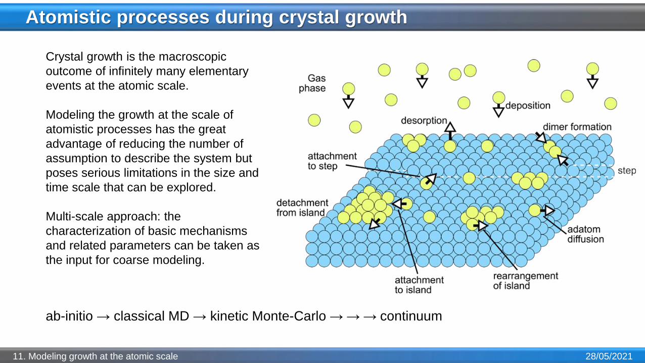
Crystal growth is the macroscopic
outcome of infinitely many elementary
events at the atomic scale.
Modeling the growth at the scale of
atomistic processes has the great
advantage of reducing the number of
assumption to describe the system but
poses serious limitations in the size and
time scale that can be explored.
Multi-scale approach: the
characterization of basic mechanisms
and related parameters can be taken as
the input for coarse modeling.
28/05/202111. Modeling growth at the atomic scale
ab-initio → classical MD → kinetic Monte-Carlo → → → continuum

Molecular dynamics
Ab-initio MD: 𝑉({𝑹}) is the eigenvalue of the ground-state electronic wave function
Classical MD: 𝑉({𝑹}) is an assigned function of the ionic coordinates. For example:
one-particle potential
(external; usually =0)
three-body potential
(angular)
pair potential
(distance)
Many-particle problem (no analytical solutions)
→ time-integration by finite differences methods
Timestep 𝜟𝒕 ≪ 𝝉 “characteristic period” of the system
The elementary processes are atomic vibrations, such that 𝝉𝒗𝒊𝒃 ∼ps.
For energy-conservation requirements, typical time steps for simulating realistic systems are of the order of fs.
Ab-initio MD up to 104 steps (10ps) Classical MD up to 109 steps (µs)
𝑉 𝑹 = 𝑉0 +
𝑖
𝑉1 𝑹𝑖 +1
2
𝑖,𝑗
𝑗≠𝑖
𝑉2 𝑹𝑖 , 𝑹𝑗 +1
6
𝑖,𝑗,𝑘
𝑘≠𝑗≠𝑖
𝑉3 𝑹𝑖 , 𝑹𝑗 , 𝑹𝑘
𝑚𝑖
𝜕2𝑹𝑖
𝜕𝑡2= −𝛻𝑖𝑉 𝑹NEWTON LAW
Evolution of the nuclei
according to the classical
hamiltonian:
𝑯 = 𝑲+ 𝑽({𝑹})
e.g. Lennard-Jones,
Morse potential. Ok for
metals (insaturate bonds)
e.g. Tersoff potential
Covalent systems with
strict bond angles
Configuration at
time 𝑡Configuration at
time 𝑡 + Δ𝑡algorithm
28/05/202111. Modeling growth at the atomic scale

Atomistic modeling of deposition
28/05/202111. Modeling growth at the atomic scale
Atom flying in the gas phase.
No perturbation of the surface
Atomic deposition:
• stochastic (random location)
• local (only the impact region is affected)
Atom impacts the surface. Their
kinetic energy is to be dissipated:
THERMALIZATION
Atom starts interacting
with the surface
𝒗
~10Å; t~ps
𝐯

𝜎 → 𝜃
𝑃 ℎ, 𝜃 →𝜃ℎ
ℎ!𝑒−𝜃 POISSON DISTRIBUTION
Stick-Where-You-Hit (SWYH) deposition
28/05/202111. Modeling growth at the atomic scale
• Probability of deposition at site 𝑖: 𝑝 = 1/𝑁
• Probability of ℎ atoms at site 𝑖 after deposition of
𝑡 atoms: BINOMIAL DISTRIBUTION
𝑃 ℎ, 𝑡 =ℎ𝑡
𝑝𝑡 1 − 𝑝 𝑡−ℎ
Thermodynamic limit 𝑁 → ∞:
ℎ =
ℎ=0
𝑡
ℎ𝑃(ℎ, 𝑡) = 𝑡𝑝 = 𝑡/𝑁 = 𝜃
𝜎2 =
ℎ=0
𝑡
ℎ − ℎ 2𝑃(ℎ, 𝑡) = 𝑡𝑝(1 − 𝑝) = 𝜃 1 −1
𝑁
Atoms land randomly on the lattice sites and stick there. T=0 K regime (no diffusion)
Disordered growth:
roughness monotonously increases
roughness

Adatom diffusion
28/05/202111. Modeling growth at the atomic scale
Courtesy by L. Barbisan
All atoms in the crystal vibrate around their equilibrium positions
(𝜈0~1013 Hz).
Diffusion is the (rare) event causing a change in the residence site
of one atom.
Let us see for example the dynamics of a Si adatom on top of the
unreconstructed (111) surface, by MD simulation (Tersoff potential)
[11ത2]
Total time 300ps – 1400K

Adatom diffusion
28/05/202111. Modeling growth at the atomic scale
Courtesy by L. Barbisan
All atoms in the crystal vibrate around their equilibrium positions
(𝜈0~1013 Hz).
Diffusion is the (rare) event causing a change in the residence site
of one atom.
Let us see for example the dynamics of a Si adatom on top of the
unreconstructed (111) surface, by MD simulation (Tersoff potential)
The trajectory in the phase-
space is stochastic in nature
and passes through
intermediate and metastable
states which are not easy to
identify a priori. The most-
likely transition path passes
through the lowest activation
barriers, i.e. the saddle points
in the potential, generally not
known a priori.Sketch of the potential curve
[11ത2]
Total time 300ps – 1400K

Adatom diffusion: time-scale separation
28/05/202111. Modeling growth at the atomic scale
𝜏vib = 1/𝜈0 ∼0.1 ps
𝜏dif ≳ 10 ns
𝜏𝛷 ∼ 1/𝐿 ∼ s-min
The system spends most of its time vibrating around an equilibrium position, and only occasionally it
moves to a new site.
→ Time-scale separation (huge at experimental conditions (t~s), negligible at high temperatures, where
the picture does not hold)
𝑘1 = 𝜈0e−EB1𝑘𝑇
𝑘2 = 𝜈0e−EB2𝑘𝑇
The MD dynamics gives us more than what we really need to understand the surface processes: it fully
traces the thermal vibrations of the adatom in any basin of minimum energy, even if this is not making any
change to the surface configuration. Can we just focus on the relevant diffusion/deposition dynamics?

𝑘 = 𝜈0 exp −𝐸𝐵𝑘𝑇
Harmonic Transition State Theory
28/05/202111. Modeling growth at the atomic scale
Hypothesis:
• Parabolic approximation of the potential
• No recrossing of the barrier once overtaken
• Adatom thermalization at ech site between the jumps
(no long jumps) → Uncorrelated diffusion events: the
system loses memory of its history by the random
vibrations around the equilibrium site
Arrhenius relation
𝑨 𝑩
𝑝 𝜏 = 𝑘e−𝑘𝜏
From statistics, the escape-time 𝝉 at which the stochastic process 𝐴 → 𝐵, with rate 𝑘, occurs follows the
exponential probability distribution:
𝑘 = 𝑘𝐴→𝐵 = event rate = number of times the event occurs in a unit time
energy of the saddle-point separating state
𝑨 and state 𝑩. It is the activation energy (or
diffusion barrier) for the event that causes
the system to move from 𝑨 to 𝑩frequency prefactor,
i.e. attempt frequency
𝜏 = escape time = time after which the event occurs for the first time

Adatom diffusion: rate
28/05/202111. Modeling growth at the atomic scale
𝑘dif = 𝑁nn 𝜈0 exp −𝐸dif
𝑘𝑇Average diffusion-time = 𝜏 = 1/𝑘dif
Hyp: jump to all equivalent nearest-
neighbour site
1D surface: 𝑁nn = 2 n.n.
2D FCC surface: 𝑁nn = 4 n.n.
2D HEX surface: 𝑁nn = 6 n.n.
All atoms in the crystal are vibrating around their equilibrium positions (𝜈0~1013 Hz).
Diffusion is the (rare) event causing a change in the residence site of one atom.
Typically: 𝐸dif ∼eV, 𝑇 ∼1000K → 𝑘dif ∼ 108 Hz ≪ 𝜈0 (Rare event!)
𝜏dif ≥ 10ns
𝐸𝐵 is strongly dependent on the atom coordination: 𝑘(bulk atom) ≪ 𝑘(complete surface layer) ≪ 𝑘(adatom)

Diffusion rate and random-walk
28/05/202111. Modeling growth at the atomic scale
Einstein theory:
Random-walk between lattice sites
Ԧ𝑟 𝑡 − Ԧ𝑟 0 2 = 𝑘dif𝑎2𝑡 = 𝑁dif𝐷𝑡
100000 diffusion steps on a square lattice
It holds true as an
ensemble average
over a large
number of random
walk trajectories
(here 100 or 1000)!
Let us consider the erratic motion of a single adatom on a planar surface, hopping between nearest-neighoring
sites on a square lattice.
𝐷 =𝑘dif𝑎
2
𝑁dif= 𝜈0𝑎
2 exp −𝐸dif𝑘𝑇
𝑘dif𝑎2𝑡
Diffusion coefficient

Diffusion vs. adsorption/desorption
𝑘dif = 𝑁𝑑 𝜈0dif exp −
𝐸dif
𝑘𝑇𝜏ads−1 = 𝜈0
ads exp −Eads
𝑘𝑇
𝜆 = 𝐷𝜏 = 𝜆0 exp𝐸ads − 𝐸dif
2𝑘𝑇
𝜈0𝑎𝑑𝑠 ∼vibrational frequency of adatoms,
normal to the surface
28/05/202111. Modeling growth at the atomic scale
𝜆0 =𝜈0𝑑𝑖𝑓
𝜈0𝑎𝑑𝑠
𝑎
𝑁𝑑
Adatoms on the surface are not expected to stay there and randomly move forever. During their erratic
motion they can interact with each other, eventually returning nucleation of critical clusters, they can
aggregate to existing islands or get captured at steps. Even if none of these happen, an adatom after a
certain time 𝜏𝑎𝑑𝑠 will be lost, because of adsorption in the crystal bulk or desorption back in the gas phase.
Diffusion
regime
Kinetic
regime

Adatom diffusion at island edges or terrace steps
28/05/202111. Modeling growth at the atomic scale
Atoms are stabilized by the interaction with neighbors as they form bonds with them.

Alternative kinetic pathways
28/05/202111. Modeling growth at the atomic scale
Fast diffusion of
the adatom across
the surface while
the island is
virtually frozen
(on the typical
adatom time scale)
2D
3D
?Interaction with other adatoms
on the surface, e.g. added by
deposition (especially at high
supersaturation).
possible nucleation
center for a new island

From MD to KMC
28/05/202111. Modeling growth at the atomic scale
MD trajectories are set on the continuum
potential energy surface. Most of the
time is spent around the minima and
only at certain times the system escape
from one basin and fall into the next one.
Representative states corresponds
to regions of the potential energy
surface pertaining to a single basin.
Each of them is distinguished as an
element in a lattice of configurations
The continuum MD trajectory
connecting the different configurations
in the lattice is replaced by a Markov
chain of discrete hops between each
state in the lattice.
Kinetic Monte Carlo is a method for visiting the phase space by following a Markov chain of hops between the
distinct configurations of the system, in a statistically consistent way. The temporal sequence of events is
tracked by knowing the full catalog of mechanisms and the corresponding rates of occurence.
Andersen, Panosetti and Reuter. Front. Chem. 7, 202 (2009) ; Voter Phys. Rev. B 34, 6819 (1986); Fichthorn & Weinberg J. Chem. Phys. 95, 1090 (1991)
Voter, “Introduction to the Kinetic Monte Carlo Method”, in Radiation Effects in Solids,(Springer, NATO Publishing Unit, Dordrecht, The Netherlands, 2005)

Let us consider two events with different activation barriers, i.e. different rates.
For each event alone, the probability that it
occurs after a time 𝜏 is:
𝑝1 𝜏 = 𝑘1e−𝑘1𝜏
𝑝2 𝜏 = 𝑘2e−𝑘2𝜏
An escape time for both rare-events can be obtained by extracting a random number for each of them,
following the exponential distribution:
𝜏1 =𝑙𝑛𝜉1𝑘1
; 𝜏2 =𝑙𝑛𝜉2𝑘2
𝜉𝑖 = rand 0,1
The evolution will then follow the path corresponding to the shortest escape time. The selected 𝜏𝑖 is
indeed the correct escape-time of event 𝑖-th since all other mechanisms has not occurred yet.
This suggests a route for implementing an algorithm to evolve the system in time.
Multiple concurrent events
28/05/202111. Modeling growth at the atomic scale
𝑘1 = 𝜈0e−EB1𝑘𝑇
𝑘2 = 𝜈0e−EB2𝑘𝑇

KMC evolution: initial state
28/05/202111. Modeling growth at the atomic scale
= empty
= filled
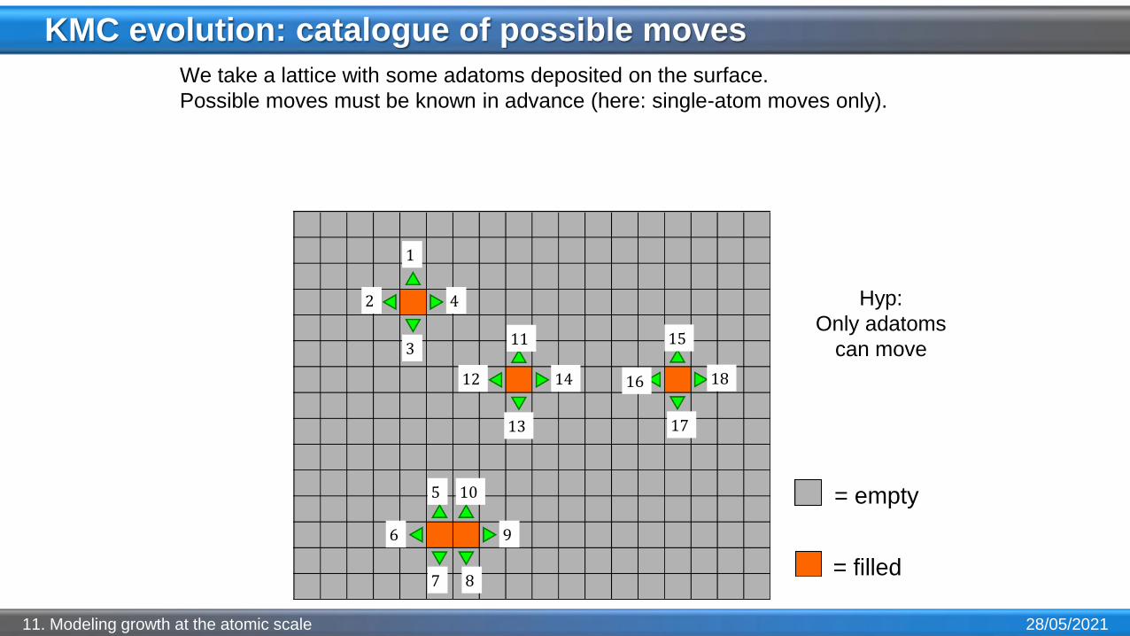
We take a lattice with some adatoms deposited on the surface.
Hyp:
Only adatoms
can move
KMC evolution: catalogue of possible moves
28/05/202111. Modeling growth at the atomic scale
We take a lattice with some adatoms deposited on the surface.
Possible moves must be known in advance (here: single-atom moves only).
1
4
3
2
11
12
13
15
17
1814
96
105
87
16
= empty
= filled
Hyp:
Only adatoms
can move

KMC evolution: catalogue of rates
28/05/202111. Modeling growth at the atomic scale
We take a a lattice with some adatoms deposited on the surface.
Possible moves must be known in advance (here: single-atom moves only).
The corresponding rates are then computed 𝑘𝑖 = 𝜈0,𝑖 exp(−𝐸𝑖/𝑘𝑇).
𝑘1
𝑘4
𝑘3
𝑘2
𝑘11
𝑘12
𝑘13
𝑘15
𝑘17
𝑘18𝑘14
𝑘9𝑘6
𝑘10𝑘5
𝑘8𝑘7
𝑘16
= empty
= filled
Hyp:
Only adatoms
can move

KMC evolution: catalogue of escape-times
28/05/202111. Modeling growth at the atomic scale
0.1ms
0.13ms
0.09ms
0.14ms
0.065ms
0.07ms
0.12ms
0.11ms
0.09ms
0.1ms0.1ms
179ms201ms
0.15ms0.17ms
0.09ms0.13ms
0.09ms
We take a a lattice with some adatoms deposited on the surface.
Possible moves must be known in advance (here: single-atom moves only).
The corresponding rates are then computed 𝑘𝑖 = 𝜈0,𝑖 exp(−𝐸𝑖/𝑘𝑇).
A random escape-time 𝜏𝑖 = −ln 𝜉𝑖/𝑘𝑖 is computed for each mechanism 𝑖. 𝜉𝑖 = rand 0,1
= empty
= filled
Hyp:
Only adatoms
can move
KMC evolution: selection of the move
28/05/202111. Modeling growth at the atomic scale
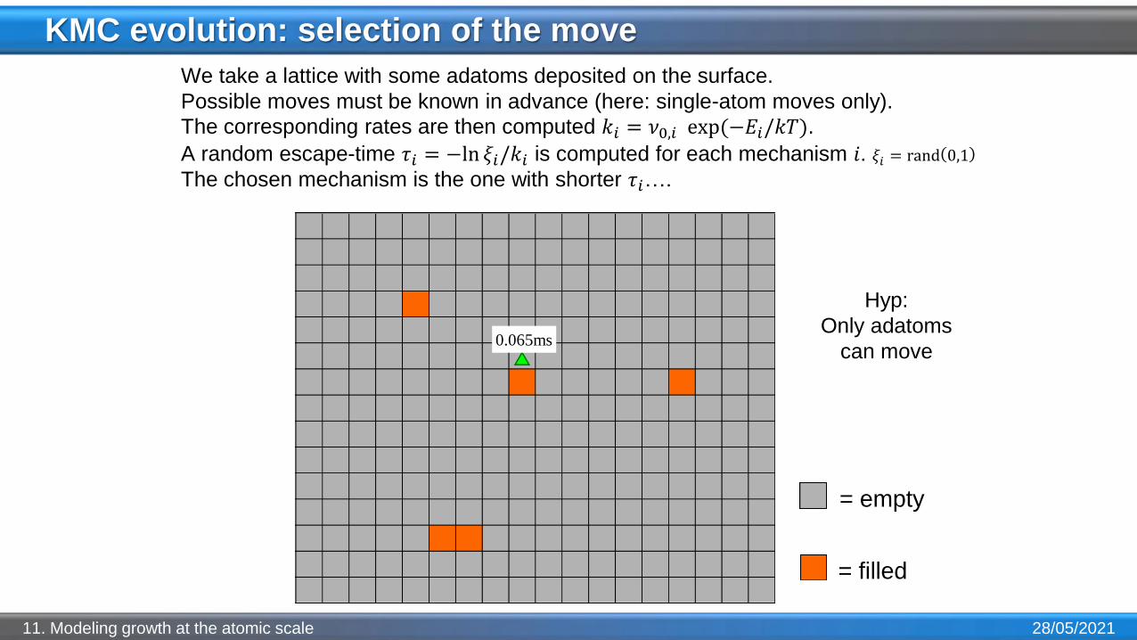
We take a lattice with some adatoms deposited on the surface.
Possible moves must be known in advance (here: single-atom moves only).
The corresponding rates are then computed 𝑘𝑖 = 𝜈0,𝑖 exp(−𝐸𝑖/𝑘𝑇).
A random escape-time 𝜏𝑖 = −ln 𝜉𝑖/𝑘𝑖 is computed for each mechanism 𝑖. 𝜉𝑖 = rand 0,1
The chosen mechanism is the one with shorter 𝜏𝑖….
0.065ms
= empty
= filled
Hyp:
Only adatoms
can move

KMC evolution: move and new state
28/05/202111. Modeling growth at the atomic scale
We take a a lattice with some adatoms deposited on the surface.
Possible moves must be known in advance (here: single-atom moves only).
The corresponding rates are then computed 𝑘𝑖 = 𝜈0,𝑖 exp(−𝐸𝑖/𝑘𝑇).
A random escape-time 𝜏𝑖 = −ln 𝜉𝑖/𝑘𝑖 is computed for each mechanism 𝑖. 𝜉𝑖 = rand 0,1
The chosen mechanism is the one with shorter 𝜏𝑖…. and the system is evolved in a new state.
= empty
= filled
Hyp:
Only adatoms
can move
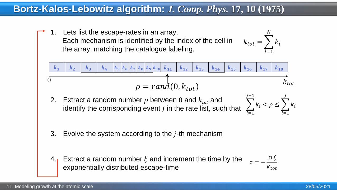
Bortz-Kalos-Lebowitz algorithm: J. Comp. Phys. 17, 10 (1975)
28/05/202111. Modeling growth at the atomic scale
𝒌𝟏 𝒌𝟐 𝒌𝟑 𝒌𝟒 𝒌𝟏𝟏 𝒌𝟏𝟐 𝒌𝟏𝟑 𝒌𝟏𝟒 𝒌𝟏𝟓 𝒌𝟏𝟔 𝒌𝟏𝟕 𝒌𝟏𝟖𝒌𝟓 𝒌𝟔 𝒌𝟕 𝒌𝟖 𝒌𝟗 𝒌𝟏𝟎
0
2. Extract a random number 𝜌 between 0 and 𝑘𝑡𝑜𝑡 and
identify the corrisponding event 𝑗 in the rate list, such that
3. Evolve the system according to the 𝑗-th mechanism
4. Extract a random number 𝜉 and increment the time by the
exponentially distributed escape-time
𝑘𝑡𝑜𝑡 =
𝑖=1
𝑁
𝑘𝑖
1. Lets list the escape-rates in an array.
Each mechanism is identified by the index of the cell in
the array, matching the catalogue labeling.
𝑘𝑡𝑜𝑡𝜌 = 𝑟𝑎𝑛𝑑 0, 𝑘𝑡𝑜𝑡
𝑖=1
𝑗−1
𝑘𝑖 < 𝜌 ≤
𝑖=1
𝑗
𝑘𝑖
𝜏 = −ln 𝜉
𝑘𝑡𝑜𝑡

KMC of thin-film growth: the solid-on-solid (SOS) model
28/05/202111. Modeling growth at the atomic scale
Constitutive assumptions:
• No vacancies
• No out-of lattice positions (no interstitials/over-coordinated sites)
• Surface configuration ℎ = ℎ 𝑖, 𝑗• Cubic lattice (extensible/mappable to other lattices)
• Only and all the topmost atom on each column ℎ are active
It is sufficient to keep track of the top exposed layers and of the
nearest neighbour list and one immediately builds on the fly the list
of mechanisms to be used in KMC. The key processes to be
modelled are:
• Deposition → stick-where-you-hit or more complex rules
(eventually desorption)
• Surface diffusion → energy barrier
SOS KMC is extremely fast and allows to match typical experimental time scales at typical temperatures,
also for rather large systems!
Young & Schubert JCP 1965; Gordon JCP 1968; Abraham and White JAP 1970; Gilmer & Bennema
JAP 1972; Vvedensky et al. 1987 and later (important modification for treating semiconductors)
𝐸𝐵 𝑖, 𝑗 = 𝐸0 + 𝑛1 𝑖, 𝑗 𝐸1 + 𝑛2 𝑖, 𝑗 𝐸2
1st neighbors 2nd neighbors
Hyp: 𝐸𝐵 depends on the
energy of the starting site
and not on the arrival one

Homoepitaxial growth on a flat surface
28/05/202111. Modeling growth at the atomic scale
Layer-by-layer: adatoms have sufficient time
to migrate and attach at the borders of existing
2D islands before nucleating a new layer
Multi-layer growth: adatom diffusion is limited so
that new nuclei form on top of incomplete layers
T=600KT=800K
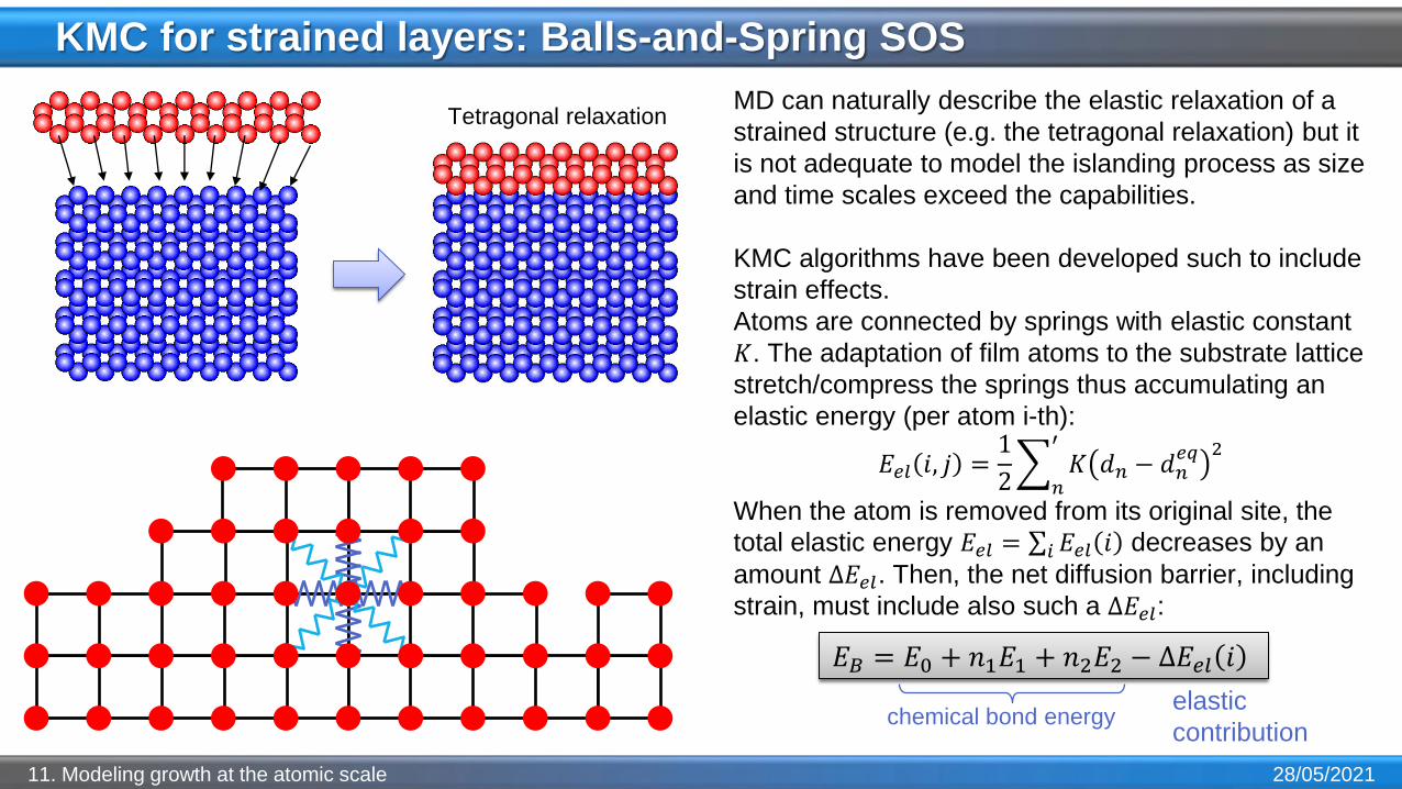
𝐸𝐵 = 𝐸0 + 𝑛1𝐸1 + 𝑛2𝐸2 − Δ𝐸𝑒𝑙 𝑖
KMC for strained layers: Balls-and-Spring SOS
28/05/202111. Modeling growth at the atomic scale
chemical bond energy
MD can naturally describe the elastic relaxation of a
strained structure (e.g. the tetragonal relaxation) but it
is not adequate to model the islanding process as size
and time scales exceed the capabilities.
KMC algorithms have been developed such to include
strain effects.
Atoms are connected by springs with elastic constant
𝐾. The adaptation of film atoms to the substrate lattice
stretch/compress the springs thus accumulating an
elastic energy (per atom i-th):
𝐸𝑒𝑙 𝑖, 𝑗 =1
2
𝑛
′
𝐾 𝑑𝑛 − 𝑑𝑛𝑒𝑞 2
When the atom is removed from its original site, the
total elastic energy 𝐸𝑒𝑙 = σ𝑖 𝐸𝑒𝑙 𝑖 decreases by an
amount Δ𝐸𝑒𝑙. Then, the net diffusion barrier, including
strain, must include also such a Δ𝐸𝑒𝑙:
elastic
contribution
Tetragonal relaxation
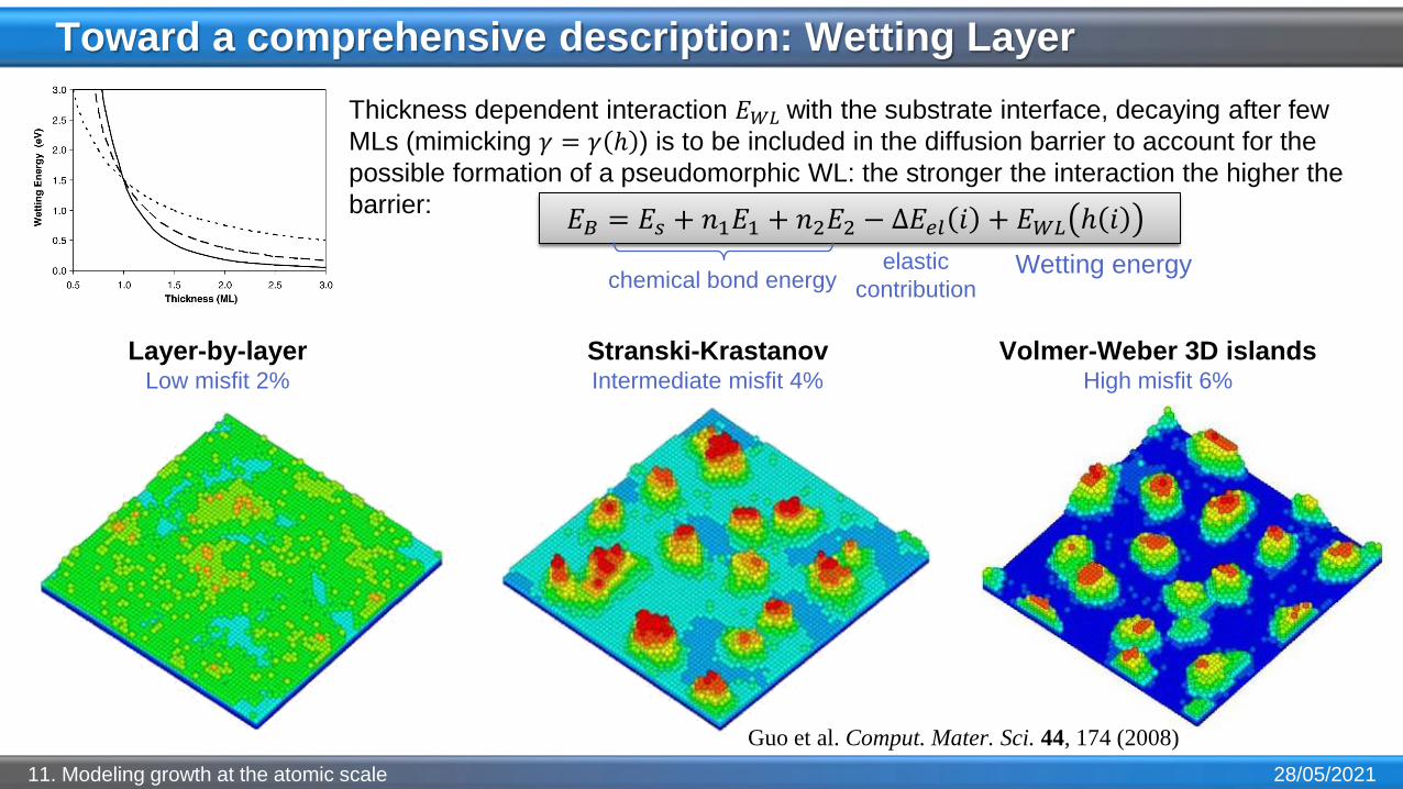
Toward a comprehensive description: Wetting Layer
28/05/202111. Modeling growth at the atomic scale
Stranski-KrastanovIntermediate misfit 4%
Layer-by-layerLow misfit 2%
𝐸𝐵 = 𝐸𝑠 + 𝑛1𝐸1 + 𝑛2𝐸2 − Δ𝐸𝑒𝑙 𝑖 + 𝐸𝑊𝐿 ℎ 𝑖
chemical bond energyelastic
contribution
Volmer-Weber 3D islandsHigh misfit 6%
Guo et al. Comput. Mater. Sci. 44, 174 (2008)
Thickness dependent interaction 𝐸𝑊𝐿 with the substrate interface, decaying after few
MLs (mimicking 𝛾 = 𝛾 ℎ ) is to be included in the diffusion barrier to account for the
possible formation of a pseudomorphic WL: the stronger the interaction the higher the
barrier:
Wetting energy