WP/16/56

Seeing in the Dark: A Machine-Learning Approach to Nowcasting in Lebanon

by Andrew Tiffin

IMF Working Papers describe research in progress by the author(s) and are published to elicit comments and to encourage debate. The views expressed in IMF Working Papers are those of the author(s) and do not necessarily represent the views of the IMF, its Executive Board, or IMF management.

© 2016 International Monetary Fund WP/16/56

IMF Working Paper

Middle East and Central Asia Department

Seeing in the Dark: A Machine-Learning Approach to Nowcasting in Lebanon

Prepared by Andrew Tiffin1

Authorized for distribution by Annalisa Fedelino

March 2016

Abstract

Macroeconomic analysis in Lebanon presents a distinct challenge. For example, long delays in the publication of GDP data mean that our analysis often relies on proxy variables, and resembles an extended version of the “nowcasting” challenge familiar to many central banks. Addressing this problem—and mindful of the pitfalls of extracting information from a large number of correlated proxies—we explore some recent techniques from the machine learning literature. We focus on two popular techniques (Elastic Net regression and Random Forests) and provide an estimation procedure that is intuitively familiar and well suited to the challenging features of Lebanon’s data.

JEL Classification Numbers: C8, C15, C44, C52, C53, C63, E3

Keywords: Macroeconomic Forecasts, Nowcasting, Random Forests, Elastic Net, LASSO, Statistical Learning, Cross Validation, Ensemble, Variable Selection, Lebanon

Author’s E-Mail Address: atiffin@imf.org

1 I am most grateful to the Lebanon team and to Adnan Mazarei for their insight, guidance, and support. In addition, particular thanks should go to Najla Nakhle from the IMF’s Beirut Office, without whom this paper would not have been possible. All errors and omissions, of course, are my own.

IMF Working Papers describe research in progress by the author(s) and are published to elicit comments and to encourage debate. The views expressed in IMF Working Papers are those of the author(s) and do not necessarily represent the views of the IMF, its Executive Board, or IMF management.

2

Contents Page

Abstract ......................................................................................................................................1 

I. Introduction ........................................................................................................................3 

II. The Nowcasting Problem: Predicting the Present ..............................................................4 

III. The Culture of Nowcasting: From Causal Inference to Machine Learning .......................5 

IV. A Regularization Approach: Elastic Net Regression .........................................................7  A. Penalized Regression ....................................................................................................7  B. LASSO and Ridge Regressions ....................................................................................7  C. The Elastic Net Regression ..........................................................................................8  D. Cross Validation ...........................................................................................................8  E. Elastic Net Regression Results for Lebanon ................................................................9 

V. A Decision-Tree Approach: Random Forests ..................................................................12  A. Decision Trees ............................................................................................................12  B. Random Forests ..........................................................................................................12  C. Random Forest Results for Lebanon ..........................................................................14 

VI. An Ensemble Approach: Putting Everything Together ....................................................15 

VII. Conclusions ......................................................................................................................16  References ................................................................................................................................17 Box 1. Regression Trees ..............................................................................................................13 Annexes 1. Elastic Net Results ............................................................................................................18 2. Random Forests Results ...................................................................................................19

3

I. INTRODUCTION

“We are drowning in information but starving for knowledge.”

Rutherford D. Roger

Macroeconomic analysis in Lebanon presents a distinct challenge. A striking example in this regard stems from the compilation and publication of Lebanon’s national-accounts: these are compiled on a yearly basis, and are published with a lag that can sometimes exceed two years. In addition, the absence of key macroeconomic data prior to 1990s—owing to the impact of the civil war—means that most economic series are relatively short and display numerous structural breaks.

Faced with an absence of timely economic statistics, discussions of economic activity tend to center around a select group of proxy measures. For example, the Banque du Liban (BdL) and the International Institute of Finance (IIF) have separately developed their own coincident indicators, which aim at taking the information contained within a range of high-frequency (monthly) variables, and combining them into a composite measure of underlying activity. The former was developed immediately following the end of the civil war and is composed of eight variables.2 And the IIF indicator follows the same approach, but includes an additional five variables.3 Most recently, the World Bank designed a new coincident indicator, which draws on the NBER Conference Board approach (Matta, 2014). All of these efforts are useful, but given that individual variables may sometimes give different (or contradictory) signals, assessments of the overall direction of the economy will often vary, depending on the methodology chosen.

The Fund has typically taken a similar coincident-indicator approach when assessing the ongoing performance of the economy. Following the BdL methodology, Staff have generally estimated real GDP using the components of the BdL’s coincident indicator—sometimes augmented by other measures of economic activity, such as construction permits, tourist arrivals, car registrations, and the number of property transactions.

This paper will outline staff’s recent efforts to augment this analysis. Framing the issue as a standard ‘nowcasting’ problem, and mindful of the pitfalls of extracting information from a large number of correlated proxy variables, the paper will draw on recent advances in machine-learning to estimate real-time movements in GDP growth.

2 These are electricity production (volumes), petroleum imports (volumes), M3 (real), cleared checks (real) total airport passenger flows (volumes), cement deliveries (volumes) and imports and export flows (real).

3 These are real private-sector credit, tourist arrivals (instead of passenger arrivals), real government revenues, real government consumption, and real machinery imports. See Iradian and Zouk (2010).

4

In particular, the paper will focus on two popular and successful machine-learning techniques—elastic-net regression and the Random Forests algorithm. It will outline the features and strengths of each approach; noting in particular that these techniques are intuitively familiar to most economists, are easily implemented, and in the particular case of Lebanese GDP, they provide plausible out-of-sample results.

II. THE NOWCASTING PROBLEM: PREDICTING THE PRESENT

The term ‘nowcasting’ is a contraction of ‘now’ and ‘forecasting,’ and has become a standard activity for central banks. Effective policymaking requires a sound assessment of economic conditions. But key measures of activity–such as GDP–generally arrive only after a delay, which essentially forces decision makers to assess current conditions by looking in the rear-view mirror. In response, central banks and other market participants have put substantial effort into providing timely assessments of GDP. The basic idea is that, by drawing on a large set of high-frequency sources (e.g., jobless figures, industrial orders, trade balance, etc.), signals about current GDP can be extracted before the associated official GDP figures are actually published. A successful nowcast will thus draw on real-time data to accurately forecast what future GDP releases will say about the current state of the economy.

The lags associated with Lebanese GDP data are sizable by international standards, but the essential problem is the same. For example, in the United States and United Kingdom, GDP data are compiled on a quarterly basis and are published approximately one month after the end of the reference quarter (so that, say, the first release of 2Q15 data will only be available end-July/early August 2015). In the euro area, the publication lag is around 2-3 weeks longer. In Lebanon, however, GDP data are compiled only on an annual basis, and the publication lag is 1-2 years—so to gauge the true state of the economy in 2015, policy makers may have to wait until 2017. Still, at a basic level the challenge across these countries is the same—given the delayed release of actual data, decision makers can exploit information published in the interim to get an ‘early estimate’ before official figures become available.

2.5

5.0

7.5

10.0

2009 2010 2011 2012 2013 2014

-3

0

3

6

9

2009 2010 2011 2012 2013 2014

GDP Growth

High Frequency Indicator

Annual Data

Long lag

5

III. THE CULTURE OF NOWCASTING: FROM CAUSAL INFERENCE TO MACHINE LEARNING

“Never trust OLS with more than five regressors”

Zvi Grilliches

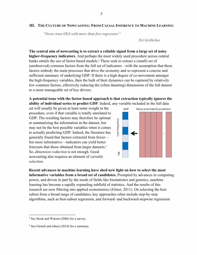
The central aim of nowcasting is to extract a reliable signal from a large set of noisy higher-frequency indicators. And perhaps the most widely used procedure across central banks entails the use of factor-based models.4 These seek to extract a (small) set of (unobserved) common factors from the full set of indicators—with the assumption that these factors embody the main processes that drive the economy and so represent a concise and sufficient summary of underlying GDP. If there is a high degree of co-movement amongst the high-frequency variables, then the bulk of their dynamics can be captured by relatively few common factors, effectively reducing the (often daunting) dimensions of the full dataset to a more manageable set of key drivers.

A potential issue with the factor-based approach is that extraction typically ignores the ability of individual series to predict GDP. Indeed, any variable included in the full data set will usually be given at least some weight in the procedure, even if that variable is totally unrelated to GDP. The resulting factors may therefore be optimal at summarizing the information in the dataset, but may not be the best possible variables when it comes to actually predicting GDP. Indeed, the literature has generally found that factors extracted from fewer—but more informative—indicators can yield better forecasts that those obtained from larger datasets.5 So, dimension reduction is not enough. Good nowcasting also requires an element of variable selection.

Recent advances in machine learning have shed new light on how to select the most informative variables from a broad set of candidates. Prompted by advances in computing power, and driven in part by the needs of fields like biostatistics and genetics, machine learning has become a rapidly expanding subfield of statistics. And the results of this research are now filtering into applied econometrics (Elmer, 2011). On selecting the best subset from a broad range of candidates, key approaches often include step-by-step algorithms, such as best-subset regression, and forward- and backward-stepwise regression

4 See Stock and Watson (2006) for a survey.

5 See Girardi and others (2014) for a summary.

6

(see Hastie and others, 2013). But these can often be computationally expensive, particularly for large datasets.

An alternative (relatively popular) approach is instead to use a type of penalized regression like elastic net regression. The advantages of the latter approach is that it is (i) intuitively familiar, (ii) entails the same (minimal) computational cost as standard OLS regression, (iii) combines dimension reduction and variable selection in a single step, and (iv) provides results that are robust to potential correlation between predictors.

Another alternative is to use a decision-tree approach, like Random Forests, which can quickly sort through a wide range of possible predictors to provide a similarly parsimonious model that copes well with possible nonlinearities and interactions. Both of these approaches will be covered in more detail below.

Machine-learning techniques are gaining ground among econometricians, and are particularly well suited to the nowcasting problem. Traditionally, econometrics and machine learning have focused on different types of problems, and have developed separately.6 Econometrics has generally focused on explanation, with particular attention to issues of causality, and a premium placed on models that are easy to interpret. A “good” model in this framework is mostly assessed on the basis of statistical significance and in-sample goodness-of-fit. Machine learning, on the other hand, has focused more on prediction, with emphasis instead on a model’s accuracy rather than its interpretability. A “good” machine-learning model, then, is often determined by looking at its likely out-of-sample success, based on bootstrap-style simulation techniques.

Despite their differences, the overlap between these two fields is growing, particularly with the arrival of “big data.” Indeed, a number of authors are currently exploring ways in which machine-learning techniques can shed light on questions of causation (Athey and Imbens, 2015). But the overlap is perhaps clearest when it comes to nowcasting, where issues of causality are less relevant. Recall, the goal of nowcasting is to extract a common signal from a broad range of indicators, with the aim of predicting what future GDP figures will say about the current environment. For this purpose, it does not matter whether an indicator reflects a causal factor that shapes GDP, or whether it is instead a symptom of GDP growth. What matters is simply that the indicator contains information about the current state of the economy, and that this information can be used in predicting the eventual GDP release. This is precisely the type of problem that machine-learning techniques are designed to address. The remainder of the paper will introduce some key concepts and algorithms within the machine-learning field, and explore their usefulness in nowcasting Lebanese GDP.

6 See Breiman (2001a) for a discussion on the different cultures associated with the two fields.

7

IV. A REGULARIZATION APPROACH: ELASTIC NET REGRESSION

“LASSO is the new OLS”

Andrew Gelman

A. Penalized Regression

Fitting is easy, prediction is hard. And prediction is particularly challenging in circumstances where there are a large number of correlated regressors. In these cases, estimated coefficients are often unstable, shifting significantly with the addition of new observations or predictors (the “bouncing beta” problem). For prediction purposes, then, out-of-sample performance will often be relatively poor, even when in-sample performance seems solid and the model is theoretically unbiased. As a solution, it is sometimes possible to find a deliberately biased model with lower prediction error than an unbiased model—giving rise to the so-called bias-variance tradeoff. One option is to add a small penalty to the usual OLS regression, which slightly biases all coefficients towards zero, but which also has the benefit of stopping them from swinging wildly in the face of new information. This is called regularization in the machine-learning literature. Different types of penalty will have different properties, and we outline some of these below.

B. LASSO and Ridge Regressions

Ridge regression is very similar to least squares, except that the coefficients are estimated by minimizing a slightly adjusted quantity. As with least squares, ridge regression seeks coefficients that fit the data well, by making the residual sum of squares (RSS) as small as possible. However, the regression also seeks to minimize a second term—called a shrinkage penalty—which is small when the regression coefficients are close to zero. This term will thus tend to shrink the coefficient estimates towards zero. The details of the penalty are provided below (where n is the number of observations, and p is the number of candidate predictors). Importantly, the tuning parameter λ serves to control the relative impact of the penalty term. When λ = 0, the penalty has no effect, and ridge regression will produce the least-squares estimates. But, as λ gets larger, the impact of the shrinkage penalty grows, and the coefficient estimates will approach zero. Unlike least squares, which

8

generates only one set of estimates, ridge regression will produce a different set of coefficients for each value of λ. So selecting a good value for λ is critical; and will be addressed in the section on cross validation below.

LASSO regression (Least Absolute Shrinkage and Selection Operator) is similar to the ridge regression, but has a different penalty. As with ridge regression, the LASSO shrinks the coefficient estimates towards zero. However, in the case of the LASSO, the penalty has the effect of forcing some of the coefficients to be exactly equal to zero when the tuning parameter λ is large enough—in contrast to the ridge regression, which may shrink coefficients so that they are close to zero, but will never eliminate them altogether. Hence, like some of the stepwise approaches outlined above, the LASSO includes an element of variable selection, and will tend to produce a parsimonious model with fewer predictors.

C. The Elastic Net Regression

The elastic net regression contains a hybrid of the ridge and LASSO penalties. The ridge penalty will tend to shrink all coefficients proportionately; and for closely correlated variables, it will tend to move the coefficients toward one another, without choosing among them. The LASSO penalty, on the other hand, will produce a leaner model by focusing on a small subset of those variables, and discarding the rest. Each approach has benefits, depending on the data, and there is no a priori reason to prefer one over the other.

The elastic net regression combines the strengths of both—selecting the best predictors to provide a parsimonious model, while still identifying of groups of closely correlated predictors. The relative weights of the two penalties are determined by an additional tuning variable (α). And as with the ridge and LASSO regressions, different values of the tuning parameters (α and λ) will produce different sets of coefficients. So, selecting the right parameter values is key.

D. Cross Validation

The tuning parameters are chosen to optimize the predictive ability of the regression. The technique is called cross validation, and is a way of gauging likely out-of-sample performance using only in-sample data. The basic idea is simple. Select a starting value for both α and λ. Divide the data into K folds (say,

Train Train Train TrainTest

1 2 3 4 5

9

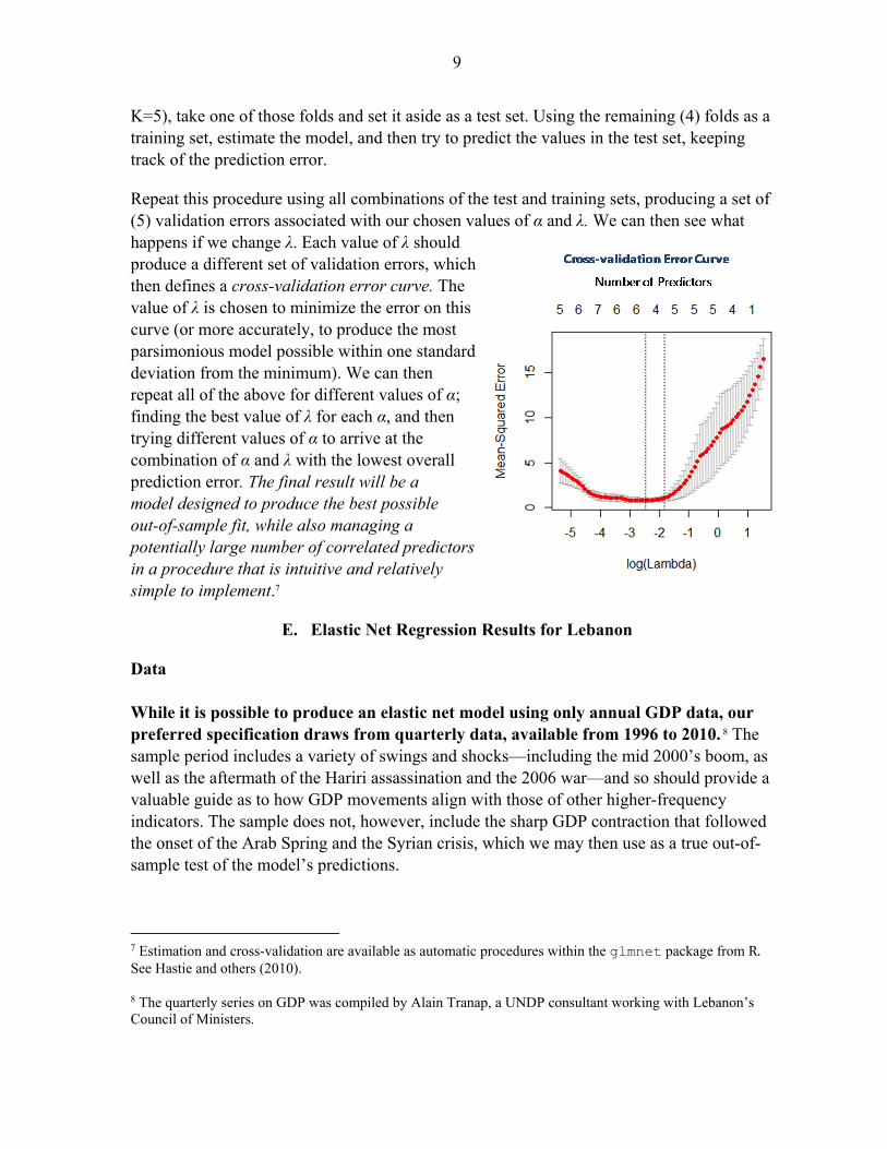
K=5), take one of those folds and set it aside as a test set. Using the remaining (4) folds as a training set, estimate the model, and then try to predict the values in the test set, keeping track of the prediction error.

Repeat this procedure using all combinations of the test and training sets, producing a set of (5) validation errors associated with our chosen values of α and λ. We can then see what happens if we change λ. Each value of λ should produce a different set of validation errors, which then defines a cross-validation error curve. The value of λ is chosen to minimize the error on this curve (or more accurately, to produce the most parsimonious model possible within one standard deviation from the minimum). We can then repeat all of the above for different values of α; finding the best value of λ for each α, and then trying different values of α to arrive at the combination of α and λ with the lowest overall prediction error. The final result will be a model designed to produce the best possible out-of-sample fit, while also managing a potentially large number of correlated predictors in a procedure that is intuitive and relatively simple to implement.7

E. Elastic Net Regression Results for Lebanon

Data While it is possible to produce an elastic net model using only annual GDP data, our preferred specification draws from quarterly data, available from 1996 to 2010. 8 The sample period includes a variety of swings and shocks—including the mid 2000’s boom, as well as the aftermath of the Hariri assassination and the 2006 war—and so should provide a valuable guide as to how GDP movements align with those of other higher-frequency indicators. The sample does not, however, include the sharp GDP contraction that followed the onset of the Arab Spring and the Syrian crisis, which we may then use as a true out-of-sample test of the model’s predictions.

7 Estimation and cross-validation are available as automatic procedures within the glmnet package from R.See Hastie and others (2010).

8 The quarterly series on GDP was compiled by Alain Tranap, a UNDP consultant working with Lebanon’s Council of Ministers.

10

For predictors, we extend the components of the BdL coincident indicator. The data are available on a monthly basis from 1996 and include the following 19 variables:

Candidate Predictor Variables

Tobacco Excises (real) Total Cleared Checks (real)

Tourist Arrivals (number) Total Airport Passenger Flows (number)

Lending to the Private Sector (real) Cement Deliveries (volumes)

Property Taxes (real) Trade flows (imports plus exports, in real terms)

Administrative Fees (real) Construction Permits (sq. m)

Primary Fiscal Spending (real) M3 (real)

Total Non-Resident Deposits (real) Port of Beirut Freight, Incoming (volumes)

Electricity Production (volumes) Port of Beirut Freight, Outgoing (volumes)

Imports of Petroleum Derivatives (volumes) Imports of Machinery (volumes)

Customs Revenue (real)

Correlation Matrix

-1 -0.8 -0.6 -0.4 -0.2 0 0.2 0.4 0.6 0.8 1

Ma

chin

e I

mp

ort

sC

em

en

tP

ort

Ou

tflo

ws

Tra

de

Po

rt I

nflo

ws

Cle

are

d C

he

cks

Co

nst

ruct

ion

Pro

pe

rty

Ta

xT

ou

rist

sP

ass

en

ge

rsC

ust

om

sE

lect

rici

tyP

etr

ol I

mp

ort

sM

3P

rim

ary

Exp

en

d.

No

n-r

es.

De

po

sits

Ad

min

. F

ee

sC

red

itT

ob

acc

o

Machine ImportsCement

Port OutflowsTrade

Port InflowsCleared Checks

ConstructionProperty Tax

TouristsPassengers

CustomsElectricity

Petrol ImportsM3

Primary Expend.Non-res. Deposits

Admin. FeesCredit

Tobacco

11

Looking at the correlation matrix for the data, a number of these series indeed seem to be tightly correlated (as expected), suggesting that trading off between bias and variance, as outlined above, may indeed improve the performance of the model. Where volume data is unavailable, nominal values are deflated by CPI to produce data series in constant prices. The regression is specified in growth rates, as this is the immediate measure of interest for Fund staff.

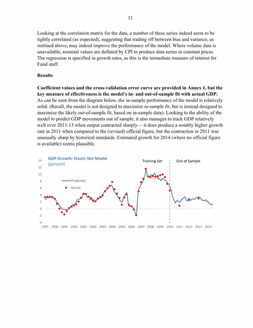
Results Coefficient values and the cross-validation error curve are provided in Annex 1, but the key measure of effectiveness is the model’s in- and out-of-sample fit with actual GDP. As can be seen from the diagram below, the in-sample performance of the model is relatively solid. (Recall, the model is not designed to maximize in-sample fit, but is instead designed to maximize the likely out-of-sample fit, based on in-sample data). Looking to the ability of the model to predict GDP movements out of sample, it also manages to track GDP relatively well over 2011-13 when output contracted sharply— it does produce a notably higher growth rate in 2011 when compared to the (revised) official figure, but the contraction in 2011 was unusually sharp by historical standards. Estimated growth for 2014 (where no official figure is available) seems plausible.

-4

-2

0

2

4

6

8

10

12

14

1997 1998 1999 2000 2001 2002 2003 2004 2005 2006 2007 2008 2009 2010 2011 2012 2013 2014

Predicted

Actual

Training Set Out of SampleGDP Growth: Elastic Net Model(percent)

12

V. A DECISION-TREE APPROACH: RANDOM FORESTS

“Random Forest has been the most successful general-purpose algorithm in modern times”

Jeremy Howard, President/Chief Scientist at Kaggle

A. Decision Trees

Tree-based methods provide an intuitive, easy-to-implement way of modeling non-linear relationships. At core, these methods are based on the notion of a decision tree, which aims to deliver a structured set of yes/no questions that can quickly sort through a wide set of features, and produce an accurate prediction of a particular outcome (GDP in our case). The technique is perhaps most familiar where the goal is to predict a qualitative variable (e.g. “spam” vs “non spam”) And in these cases, a traditional econometric approach would usually be to use a logit or probit model. But decision trees take a very different approach. Rather than fitting a (transformed) linear regression, they center instead around the repeated partitioning of the predictor space into two sets, starting with an initial split that decreases the prediction error the most. These binary partitions then continue until the termination of the tree, and are recursive—i.e. each subsequent split is not conducted on the entire dataset, but only on the portion of the prior split under which it falls. The result is an efficient set of questions that can quickly narrow down the likelihood of our modeled outcome falling into a particular category (“spam”) or another (“non spam”).

The decision-tree approach can predict continuous variables as well as qualitative variables. In this case, the decision tree is typically called a regression tree (Box 1) and produces a step-wise nonparametric estimator for the conditional expectation of the outcome (again, GDP in our case). Decision trees are computationally efficient, and work well for problems where there are important nonlinearities and interactions. They also are well suited to cope with missing data. Trees tend not to work very well if the underlying relationship is linear, but even in these cases they can often reveal aspects of the data that are not apparent from a traditional linear approach (Varian, 2014).

B. Random Forests

The Random Forest (RF) algorithm modifies the decision-tree approach to minimize the problem of overfitting. One problem with trees is that, like standard OLS with many correlated predictors, they often provide models that fit the training sample well, but which perform poorly when making out-of-sample predictions. A common solution to this problem is to shorten or “prune” the tree by imposing a penalty for an overly long/complex structure, analogous to the regression penalty added in the elastic net regression. The ideal degree of complexity is then chosen using cross-validation techniques. Instead of pruning, however, the RF algorithm (Breiman, 2001b) takes a different approach—seeking instead to improve the model’s predictive ability by growing numerous (unpruned) trees and combining the results.

13

Box 1. Regression Trees (continued) A regression tree is a particular type of decision tree, which designed to approximate a continuous real-valued function, rather than a yes/no classifier.

The tree is built through an iterative process that splits the data into partitions or branches, and then continues splitting each partition into smaller and smaller groups.

Initially, all observations are placed in the same group. The data is then allocated into two partitions (or branches), using every possible split on every available

predictor: the predictor/split actually chosen is the one that that most clearly separates the observations into two distinct groups, i.e. minimizes the overall deviation from the mean in each of the two separate partitions.

This splitting rule is then reapplied to each of the two new branches. The process continues until each group reaches a pre-specified minimum size (minimum node size). Having split the data (x) optimally into a (large) number of separate bins, the regression tree simply calculates

the mean value of the outcome variable (y) for each bin.

30

7

X > 30?

20 60

15

20

35

X > 20?

yes no

y = 35 y = 15

X > 60?

y = 20

yes no

yes no

y = 7

Repeat as needed

X > 20?

yes no

X > 60?

yes no

yes no

… etc …

x

x

X > 30?

30

10

30

yes no

y = 30 y = 10

x

y

y

yX > 30?

X > 30?

10

20

35

yes no

y = 35

X > 60?

y = 20

yes no

x

y

y = 10

30 60

Gro

win

g th

e r

egr

ess

ion

tre

e

14

Box 1. Regression Trees (concluded) A fully developed tree often suffers from over-fitting—the deeper the tree, the better the fit, but taken to the extreme it is possible to keep extending the tree until each individual data point is represented by its own terminal branch, resulting in a “perfect” in-sample fit. This over-fitting generally results in poor out-of-sample performance. So regression trees are often “pruned,” i.e. shortened at the expense of the in-sample fit, but with the aim of improving out-of-sample success. There is a sizable literature on how to prune regression tees optimally, which draws on many of the cross-validation techniques outlined in the main text.

Once settled, the regression tree provides a non-parametric estimate of the expected outcome (GDP), conditional on the predictors falling into a particular bin.

Essentially, the regression tree partitions the set of predictors efficiently into M regions R1, R2, …, RM. The response variable (y) is then modeled as the average for the region, with

∈

where

| ∈

The first Random Forest modification is the use of bootstrap aggregation (or “bagging”). In bagging, an individual tree is built on a random sample of the dataset, roughly two thirds of the total observations—the remaining one-third are referred to as out-of bag (OOB) observations and can be used to gauge the accuracy the tree. This is repeated hundreds or thousands of times and the results are averaged. The fact that none of the trees is pruned means that the variance of each individual tree is high. However, by averaging the results, we can reduce the variance without increasing the bias.

The second modification is to take a random sample of the set of predictors at each split. In the case of highly correlated predictors, and particularly in the event of a single driving predictor, bagging by itself can be insufficient, as it may simply produce multiple versions of essentially the same tree. To get around this problem, RF introduces an added element of randomization—at each split, the algorithm only considers a random subset of the available set of predictors (usually the total number of predictors divided by three). By randomizing the predictor space, the RF algorithm effectively guarantees that the multiple trees that go into the final collection will be relatively diverse. Each tree on its own will be a weak model, as it is grown on a deliberately limited dataset. But the essence of the RF approach is that, by combining a large number of (uncorrelated) weak models, we can end up with an aggregate prediction that is surprisingly strong.

C. Random Forest Results for Lebanon

Using the same training data as for the elastic net regression, the in-sample and out-of-sample performance of the Random Forest are also solid.9 Detailed results are

9 Estimation and cross validation are available as automatic procedures within the randomForests package in R. See Liaw and Weiner (2002).

15

provided in Annex 2, but the model’s predictions are shown in the chart below. Again, the model tracks GDP relatively well over the training sample. It also follows GDP closely over 2011-13 when output contracted sharply— although, like the elastic net, it predicts a higher growth rate in 2011 compared to the official figure. Estimated growth for 2014 (where no official figure is available) is again plausible.

VI. AN ENSEMBLE APPROACH: PUTTING EVERYTHING TOGETHER

“…and in a multitude of counselors, there is safety.”

Proverbs 24:6

Of the two models, the elastic net produces more-accurate forecasts of Lebanese GDP. Placing the cross-validation results of the two models side-by-side, and comparing their associated prediction errors, the elastic net approach seems to dominate the Random Forest approach—suggesting that the underlying relationship between our predictors and GDP may be linear.

Nonetheless, it may still be possible to combine the two models in a way that reduces the likely prediction error even further. In this context, there is a further concept in the machine learning literature—the ensemble—that may help us design an even stronger model. An ensemble is a collection of models whose predictions are combined by weighted averaging or voting. Indeed, the RF algorithm itself is an example of an ensemble technique, in which individual trees are combined (and where the accuracy of the combined prediction is greater than that of any of its component parts). Looking at our two approaches, we can consider an

Root MSE

Elastic Net 0.6902

Random Forests 1.1671

Ensemble 0.6892

Weight on Elastic Net 0.96

Weight on Random Forest 0.04

GDP Growth: Ensemble Predictor

-4

-2

0

2

4

6

8

10

12

14

1997 1998 1999 2000 2001 2002 2003 2004 2005 2006 2007 2008 2009 2010 2011 2012 2013 2014

Predicted

Actual

Training Set Out of SampleGDP Growth: Random Forest Model(percent)

16

elementary ensemble, simply by building a weighted average of the two predictions. And again, we can choose the optimal weights—those likely to give the best out-of-sample fit—by cross validation.10 From our results, although the elastic net approach is likely to be the more accurate of the two models, it seems that we can nonetheless reduce our likely prediction error (albeit marginally) by combining the two predictions and placing a (small) weight on the Random Forest model.

VII. CONCLUSIONS

Faced with long delays in the publication of official GDP data, Fund staff have often been required to assess recent trends based on various proxy variables. This note highlights the similarities between this problem, and the relatively common ‘nowcasting’ challenge addressed routinely by central banks and market participants. Drawing on the nowcasting literature, as well as some of the methodologies developed within the field of machine learning, the note has presented a procedure for GDP estimation that is both intuitively familiar, and well suited to the more challenging features of Lebanon’s data.

10 Cross validation and the calculation of optimal weights are available as automatic procedures within the caretEnsemble package in R.

-4

-2

0

2

4

6

8

10

12

14

1997 1998 1999 2000 2001 2002 2003 2004 2005 2006 2007 2008 2009 2010 2011 2012 2013 2014

EnsembleElastic NetRFActual

Training Set Out of SampleGDP Growth: Ensemble Model(percent)

17

References

Athey, S. and G.W.Imbens, 2015, “Machine Learning Methods for Estimating Heterogenous Causal Effects,” manuscript.

Breiman, L., 2001a, “Statistical Modeling: Two Cultures,” Statistical Science, Vol. 16 (3), pp.199–231, August 2001.

———, 2001b, “Random Forests,” Machine Learning, Vol. 45, pp.5–32.

Elmer, S.G., 2011, “Modern Statistical Methods Applied to Economic Time Series,” KOF Dissertation Series, No.6, 2011. Swiss Federal Institute of Technology, Zurich.

Girardi, A, R.Golinelli and C. Pappalardo, 2014, “The Role of Indicator Selection in Nowcasting Euro Area GDP in Pseudo Real Time,” Working Papers 919, Dipartimento Scienze Economiche, Universita' di Bologna.

Hastie, T., J.Friedman, and R.Tibshirani, 2009, The Elements of Statistical Learning: Data Mining, Inference, and Prediction (2nd Edition). Springer, New York.

———, 2010, “Regularization Paths for Generalized Linear Models via Coordinate Descent,” Journal of Statistical Software, Vol. 33, Issue 1, Feb 2010.

Hastie, T., G.James, D.Witten, and R.Tibshirani, 2013, An Introduction to Statistical Learning, Springer, New York.

Hastie, T., R.Tibshirani, and M.Wainwright, 2015, Statistical Learning with Sparsity: The Lasso and Generalizations, CRC Press, Boca Raton.

Iradian. G, and N. Zouk, 2010, “Lebanon: New Estimates Reveal Exceptional Growth,” Institute of International Finance, Washington DC.

Liaw, A., and M. Wiener (2002). “Classification and Regression by randomForest,” R News Vol 2 (3), pp.18–22.

Matta, S., 2014, “New Coincident and Leading Indicators for the Lebanese Economy,” World Bank Policy Research Working Paper, No. 6950. World Bank, Washington D.C.

Stock, J.H. and M.W.Watson, 2006, “Forecasting with Many Predictors,” Handbook of Economic Forecasting, Vol.1 Ch.10, pp. 515–54.

Varian, H., 2014, “Big Data: New Tricks for Econometrics,” J. of Ec. Perspectives, Vol. 28(2), pp. 3–27, Spring 2014.

18

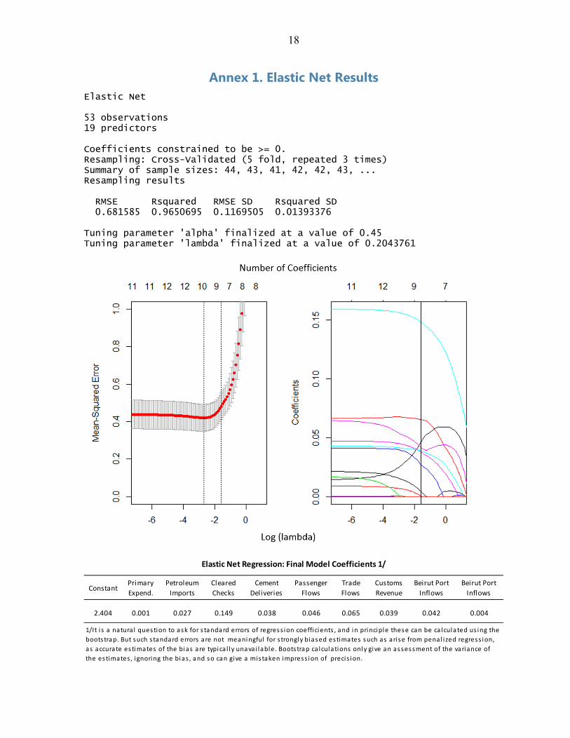
Annex 1. Elastic Net Results Elastic Net 53 observations 19 predictors Coefficients constrained to be >= 0. Resampling: Cross-Validated (5 fold, repeated 3 times) Summary of sample sizes: 44, 43, 41, 42, 42, 43, ... Resampling results RMSE Rsquared RMSE SD Rsquared SD 0.681585 0.9650695 0.1169505 0.01393376 Tuning parameter 'alpha' finalized at a value of 0.45 Tuning parameter 'lambda' finalized at a value of 0.2043761

ConstantPrimary

Expend.

Petroleum

Imports

Cleared

Checks

Cement

Deliveries

Passenger

Flows

Trade

Flows

Customs

Revenue

Beirut Port

Inflows

Beirut Port

Inflows

2.404 0.001 0.027 0.149 0.038 0.046 0.065 0.039 0.042 0.004

Elastic Net Regression: Final Model Coefficients 1/

1/It i s a natura l ques tion to as k for s tandard errors of regres s ion coefficients , and in principle thes e can be ca lculated us ing the

boots trap. But such standard errors are not meaningful for s trongly biased estimates such as arise from penal ized regress ion,

as accurate es timates of the bias are typica l ly unavai lable. Boots trap ca lculations only give an as ses sment of the variance of

the estimates , ignoring the bias , and s o can give a mis taken impress ion of precis ion.

19

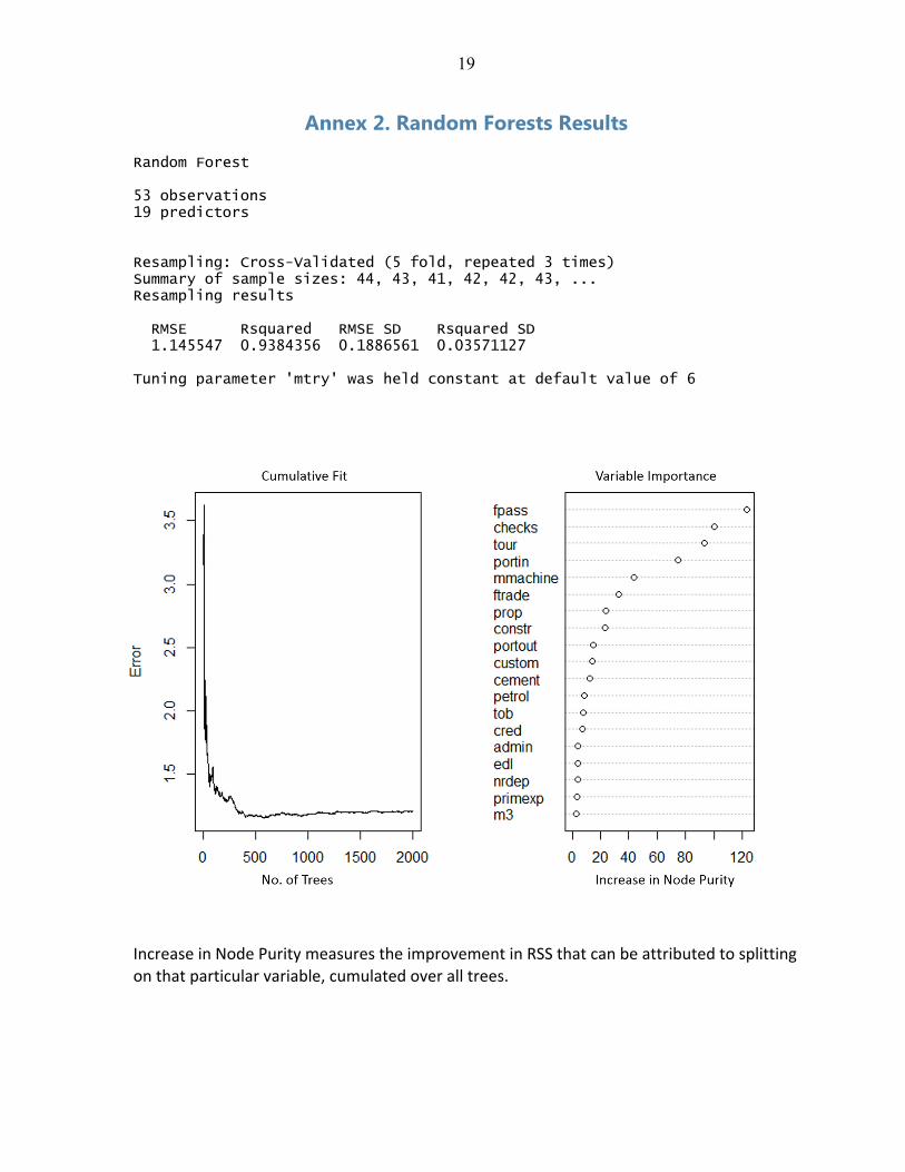
Annex 2. Random Forests Results

Random Forest 53 observations 19 predictors Resampling: Cross-Validated (5 fold, repeated 3 times) Summary of sample sizes: 44, 43, 41, 42, 42, 43, ... Resampling results RMSE Rsquared RMSE SD Rsquared SD 1.145547 0.9384356 0.1886561 0.03571127 Tuning parameter 'mtry' was held constant at default value of 6

Increase in Node Purity measures the improvement in RSS that can be attributed to splitting on that particular variable, cumulated over all trees.