section 8 development of and advances in ocean modelling

Section 8

Development of and advances in oceanmodelling and data assimilation, sea-ice

modelling, wave modelling

Numerical investigation of ocean mixed layer in response to moving cyclone of different eye radii

A.A.Deo, D.W.Ganer and P.S.Salvekar

Indian Institute of Tropical Meteorology, Pune 411 008, India

E-mail : [email protected] Introduction Present work deals with the sensitivity studies of the upper mixed layer response to an idealized Indian Ocean cyclone having different eye radii using simple ocean model. In the earlier studies the surface circulation and mixed layer depth (MLD) variation as well as temperature change has been studied in response to moving cyclones in the Indian Ocean

1,2,3,4.

The model used in this study is a simple 1½ layer reduced gravity ocean model over the tropical Indian Ocean (35°E-115°E, 30°S-25°N) with one active layer overlying a deep motionless inactive layer

3. The initial thermocline is assumed to be 50 m deep and the gravity

wave speed is 1 m/s. The initial temperature in the mixed and bottom layer are considered as 29 °C and 23 °C. Numerical experiments and discussion of results

The horizontal resolution of the model is 1/8° x 1/8°. The model cyclone assumes a

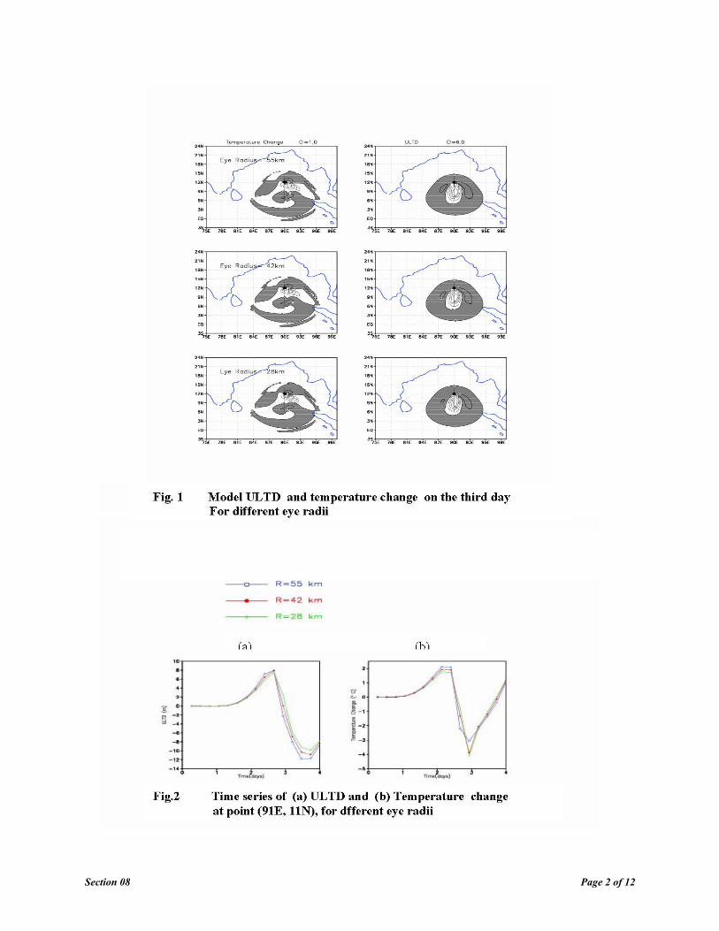
symmetric ranking vortex having radius 400 km and maximum winds 20 m/s. The radius of eye wall is taken as 55 km for control experiment and is changed to 42 km and 28 km in the sensitivity study. Such vortex is allowed to move along northward track in the Bay of Bengal in four days. The track considered is from the initial position of (90E, 6N) to (90E, 14N). The model is integrated for four days (considered life span of the cyclone), from the initial condition of rest. The variations in the upper layer thickness (ULT) and temperature from the initial conditions are studied.

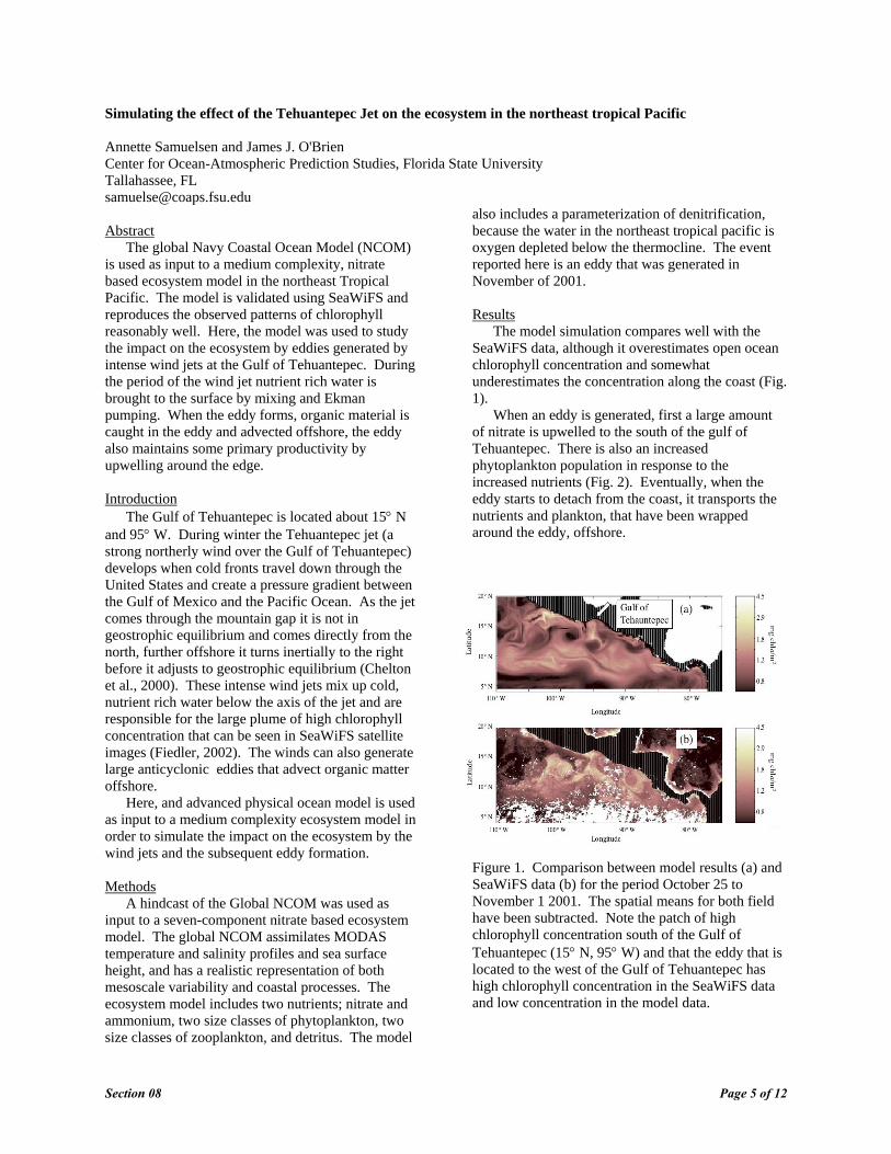
Figure 1 shows temperature change of mixed layer from the initial temperature of 29 °C (left panel) and upper layer thickness deviation (ULTD) from initial value of 50 m (right Panel), on the third day for different values of eye radius. The ULTD shows that as the radius of eye decreases, the maximum upwelling and down welling decreases. For example at the point (91 E, 11N) near the track the time series of ULTD (Figure 2a) shows the values of maximum upwelling as 12m, 11m and 10m, for eye radius 55m, 42m and 28m respectively. Model temperature field shows increase in maximum cooling and decrease in maximum warming as the eye radius decreases. This is clearly seen from figure 2b, which shows the times series of temperature change at the point (91 E, 11N) near the track. References:

1. Behera S.K, Deo A.A, and Salvekar P.S., 1998: Investigation of mixed layer response to Bay of Bengal cyclone using a simple ocean model. Meteorol. Atmos. Phys.,65, 77-91.

2. Chang S.W. & Anthes R.A., 1978: Numerical simulation of the ocean’s nonlinear baroclinic response to translating hurricanes. J. Phys. Oceano., 13, 468-480

3. Deo A.A, Salvekar P.S and Behera S.K,2001: Oceanic response to cyclone moving in different directions over Indian Seas using IRG model. Mausam, 52, 163-174.

4. Price J.F., 1981: Upper ocean response to a hurricane. J. Phys. Oceano., 11,153-175.

Section 08 Page 1 of 12

mailto:[email protected]

Modeling the Oceanic Response to Air-Sea Fluxes Associated with a Tropical Storm

Steven L. Morey, Mark A. Bourassa, Dmitry Dukhovskoy, and James J. O’Brien

Center for Ocean – Atmospheric Prediction Studies

Florida State University Tallahassee, FL 32306-2840

[email protected]

1. Introduction A new boundary layer model is used with a numerical ocean model to simulate and better understand the impacts of turbulent fluxes of heat and momentum between the ocean and atmosphere during energetic forcing events, such as tropical cyclones. In particular, the case of Tropical Storm Harvey in the Gulf of Mexico during September, 1999, is simulated and analyzed. Winds derived from the NASA SeaWinds scatterometer aboard the QuikSCAT satellite are used as input to the atmospheric flux model, along with air temperatures from an atmospheric model and sea surface temperatures from the ocean model. Experiments are run with both momentum and heat fluxes, and then with momentum and heat fluxes applied separately, to illustrate the roles that the surface forcing mechanisms play in governing the evolution of the upper ocean thermal structure. Results show that the sea surface temperature (SST) response is dominantly driven by the surface heat flux. Surface cooling also promotes a deepening of the mixed layer through convective mixing. The surface wind stress, upwelling favorable under a tropical cyclone, can enhance the surface cooling by entraining cooler deeper water into the surface mixed layer.

2. The Model The Navy Coastal Ocean Model (NCOM) (Martin 2000) has been configured to simulate the Gulf of Mexico (GoM) and northwestern Caribbean with a horizontal resolution of 1/20° in latitude and longitude as in Morey et al. (2003), but with an increase in the vertical resolution to 60 levels (20 sigma levels above 100 m and 40 z-levels below). The model assimilates MODAS (Modular Ocean Data Assimilation System, Fox et al. 2002) three-dimensional synthetic temperature and salinity profiles, and is horizontally nested within the Navy Research Laboratory 1/8° NCOM global hindcast model for lateral boundary conditions. Output from this GoM hindcast model is used for initialization of the experiments described in

this paper. No data assimilation is used during the experiments. An atmospheric flux model based on the Bourassa-Vincent-Wood (BVW) boundary layer model (Bourassa et al. 1999) is coupled to the NCOM. This flux model has the advantage of more accurately calculating air-sea fluxes dependent on the sea state, air-surface temperature and humidity difference, and 10 m wind velocity. For the experiments presented here, the flux model is used assuming local wind-wave equilibrium and a prescribed air-sea humidity difference. Calculation of the surface momentum flux, latent heat flux, and sensible heat flux then reduce to functions of the air-sea temperature difference and the 10 m wind velocity for these experiments. Air temperatures for these experiments are extracted from the European Center for Medium Range Weather Forecasting (ECMWF) Global Advanced Operational Surface Analysis and winds are derived from the SeaWinds scatterometer aboard the polar orbiting QuikSCAT satellite. The scatterometer wind data are objectively gridded using the Eta-29 atmospheric model data as a background field (Morey et al. 2004). The resulting input fields to the flux model consist of 1° air temperature and ½° 10 m winds, both at 12-hour time intervals, and NCOM SST at each model time step. The coupled model is run for September 15, 1999 – September 23, 1999.

3. Results

T.S. Harvey passed over the eastern Gulf of Mexico during September 19 – 22, 1999, making landfall along the southwest coast of the Florida peninsula. Numerical model results show that surface heat fluxes (latent and sensible) were largest coincident with the strongest winds and reached magnitudes in excess of 600 W/m2 (Figure 1). Substantial cooling associated with the tropical storm can be seen offshore of the West Florida Shelf, where the SST was reduced by more than 1.5° C (Figure 2, indicated by the arrow). A model run in which neglected wind stress (although wind speed was used in the heat flux calculations) produced similar


Fig. 1. Vector wind stress (arrows) and latent plus sensible heat fluxes (positive upward) modeled on September 20, 1999. cooling, though somewhat less pronounced in the region of maximum response to the storm. In a third experiment, the sea surface was insulated. The cooling over the basin was not as pronounced, but the SST was reduced by more than 0.6° under the path of the storm, coincident with the region of maximum cooling in the control experiment with all fluxes calculated.

Fig. 2. Sea surface temperature change from September 18 to 23, 1999. Only cooling is shaded. Top: Model run with heat and momentum fluxes. Lower Left: Model with no wind stress (momentum flux). Lower Right: Model with insulated sea surface (no heat fluxes).

The time series of the temperature profiles at the center of the most extreme cooling (indicated by the arrow in Figure 2) for each experiment show the subsurface ocean response to the tropical cyclone (Figure 3). Upwelling of the isotherms and subsequent inertia gravity waves are evident, as is the cooling of the surface mixed layer. The experiment neglecting wind

stress shows that convective mixing is responsible for maintaining the mixed layer depth, and heat loss results in cooling of the mixed layer. The experiment that neglects surface heat fluxes shows that the wind driven upwelling reduces the mixed layer depth, and entrainment of cooler water into the mixed layer also contributes to the cooling of the upper ocean.

Fig. 3. Time series of the upper 50m temperature profile near the location specified by the arrow in Figure 2. Top: Model run with heat and momentum fluxes. Lower Left: Model with no wind stress (momentum flux). Lower Right: Model with insulated sea surface (no heat fluxes).

Acknowledgements

This project was sponsored by the National Science Foundation, the Office of Naval Research Secretary of the Navy grant to James J. O'Brien, and by the NASA Office of Earth Science. Computer time was provided by the DoD High Performance Computing Modernization Office, and by the FSU Academic Computing and Network Services.

References Bourassa, M. A., D. G. Vincent, W. L. Wood, 1999: A flux

parameterization including the effects of capillary waves and sea state. J. Atmos. Sci., 56, 1123-1139.

Martin, P.J., 2000: “A description of the Navy Coastal Ocean Model Version 1.0”. NRL Report: NRL/FR/7322-009962, Naval Research Lab., Stennis Space Center, MS, 39 pp.

Morey, S. L., P. J. Martin, J. J. O’Brien, A. A. Wallcraft, and J. Zavala-Hidalgo, 2003: Export pathways for river discharged fresh water in the northern Gulf of Mexico, J. Geophys. Res., 108(C10), 3303, doi: 10.1029/2002JC001674.

Morey, S. L., M. A. Bourassa, X. J. Davis, J. J. O’Brien, and J. Zavala-Hidalgo, 2004: Remotely sensed winds for episodic forcing of ocean models, J. Geophys. Res., In review.

Fox, D.N., W.J. Teague, C.N. Barron, M.R. Carnes, and C.M. Lee, 2002: The Modular Ocean Data Assimilation System (MODAS), J. Atmos. Ocean. Tech., 19, 240-252.


Simulating the effect of the Tehuantepec Jet on the ecosystem in the northeast tropical Pacific Annette Samuelsen and James J. O'Brien Center for Ocean-Atmospheric Prediction Studies, Florida State University Tallahassee, FL [email protected] Abstract

The global Navy Coastal Ocean Model (NCOM) is used as input to a medium complexity, nitrate based ecosystem model in the northeast Tropical Pacific. The model is validated using SeaWiFS and reproduces the observed patterns of chlorophyll reasonably well. Here, the model was used to study the impact on the ecosystem by eddies generated by intense wind jets at the Gulf of Tehuantepec. During the period of the wind jet nutrient rich water is brought to the surface by mixing and Ekman pumping. When the eddy forms, organic material is caught in the eddy and advected offshore, the eddy also maintains some primary productivity by upwelling around the edge. Introduction

The Gulf of Tehuantepec is located about 15° N and 95° W. During winter the Tehuantepec jet (a strong northerly wind over the Gulf of Tehuantepec) develops when cold fronts travel down through the United States and create a pressure gradient between the Gulf of Mexico and the Pacific Ocean. As the jet comes through the mountain gap it is not in geostrophic equilibrium and comes directly from the north, further offshore it turns inertially to the right before it adjusts to geostrophic equilibrium (Chelton et al., 2000). These intense wind jets mix up cold, nutrient rich water below the axis of the jet and are responsible for the large plume of high chlorophyll concentration that can be seen in SeaWiFS satellite images (Fiedler, 2002). The winds can also generate large anticyclonic eddies that advect organic matter offshore.

Here, and advanced physical ocean model is used as input to a medium complexity ecosystem model in order to simulate the impact on the ecosystem by the wind jets and the subsequent eddy formation.

Methods

A hindcast of the Global NCOM was used as input to a seven-component nitrate based ecosystem model. The global NCOM assimilates MODAS temperature and salinity profiles and sea surface height, and has a realistic representation of both mesoscale variability and coastal processes. The ecosystem model includes two nutrients; nitrate and ammonium, two size classes of phytoplankton, two size classes of zooplankton, and detritus. The model

also includes a parameterization of denitrification, because the water in the northeast tropical pacific is oxygen depleted below the thermocline. The event reported here is an eddy that was generated in November of 2001. Results

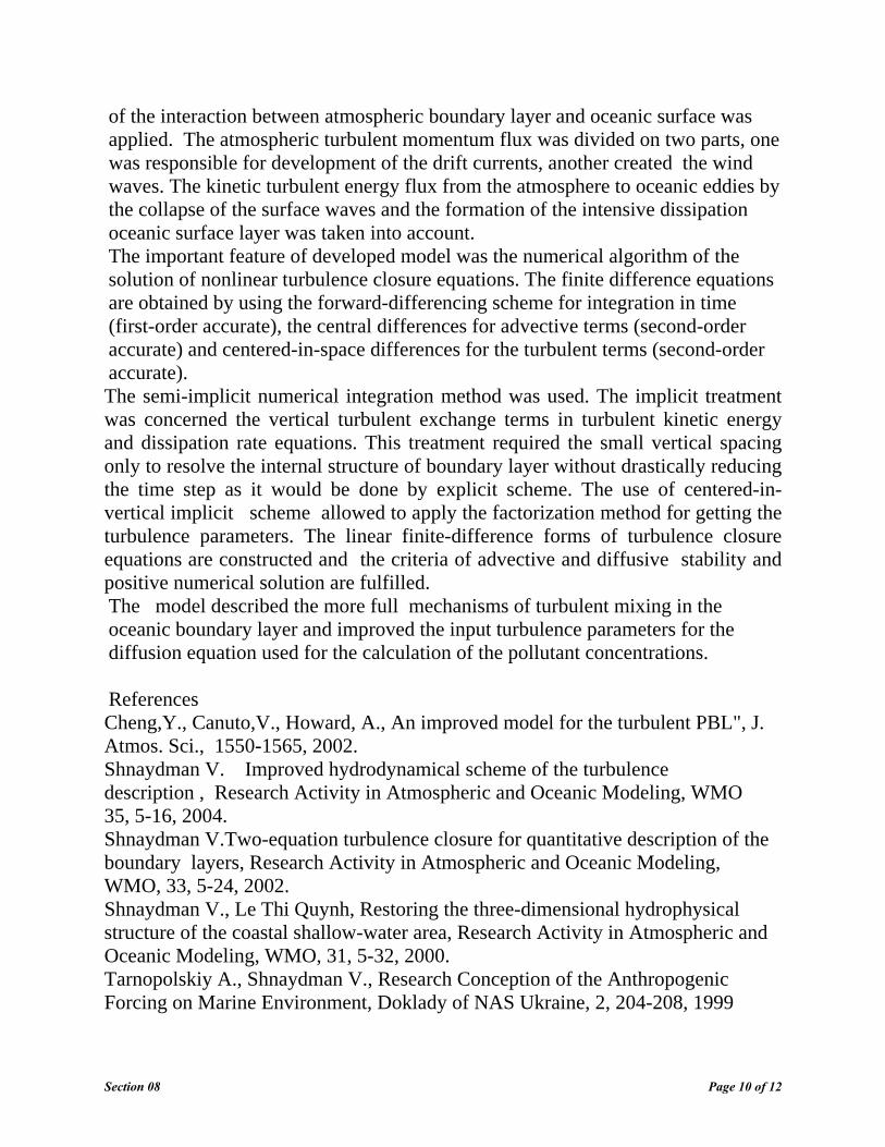
The model simulation compares well with the SeaWiFS data, although it overestimates open ocean chlorophyll concentration and somewhat underestimates the concentration along the coast (Fig. 1).

When an eddy is generated, first a large amount of nitrate is upwelled to the south of the gulf of Tehuantepec. There is also an increased phytoplankton population in response to the increased nutrients (Fig. 2). Eventually, when the eddy starts to detach from the coast, it transports the nutrients and plankton, that have been wrapped around the eddy, offshore.

Figure 1. Comparison between model results (a) and SeaWiFS data (b) for the period October 25 to November 1 2001. The spatial means for both field have been subtracted. Note the patch of high chlorophyll concentration south of the Gulf of Tehuantepec (15° N, 95° W) and that the eddy that is located to the west of the Gulf of Tehuantepec has high chlorophyll concentration in the SeaWiFS data and low concentration in the model data.



Figure 2. Generation and detachment from the coast of a eddy at the gulf of Tehuantepec. The first column displays horizontal velocity, represented by arrows, and the vertical velocity, represented by color. After the eddy is detached from the coast (25. November), it has patches of upward velocity along the edge. The second and third column show the nitrate and large phytoplankton corresponding to the eddy. Both components get caught in the eddy velocity field and are transported offshore. Discussion

The model simulated the ecosystem response to eddy generation fairly realistically and it is clear that these eddies contribute to transporting a considerable amount of organic matter offshore. Although, as the eddy propagates further offshore, the simulated data show low concentration of chlorophyll at the center of the eddy, while the satellite data show the chlorophyll is more evenly distributed across the eddy. The reason for this discrepancy is unclear, but it may be that the model overestimates the vertical velocity at the center of the eddy or the lack of horizontal diffusivity in the ecosystem model prevents the ecosystem components from spreading across the eddy.

References Chelton, D. B., M. H. Freilich, and S. K. Esbensen, 2000: Satellite observations of the wind jets off the Pacific coast of Central America. Part I: Case studies and statistical characteristics. Monthly Weather Review, 128, 1993-2018. Fiedler, P. C., 2002: The annual cycle and biological effects of the Costa Rica Dome. Deep-Sea Research Part I-Oceanographic Research Papers, 49, 321-338. Acknowledgement Chlorophyll a and PAR data were obtained from the NASA/GSFA/DAAC.


Entropy production of the oceanic general circulation

Shinya Shimokawa * and Hisashi Ozawa ** * National Research Institute for Earth Science and Disaster Prevention, Tsukuba 305-0006, Japan ([email protected])

** Hiroshima University, Higashi-Hiroshima 739-8521, Japan

1. Introduction

Ocean system is regarded as an open dissipative system connected to the surrounding system (atmosphere and the universe)

mainly through heat and salt fluxes. In this view point, the formation of a circulatory structure can be regarded as a process leading to

the final equilibrium of the whole system consisting of the ocean system and the surrounding system. In this process, the rate of

approach to the equilibrium, i.e. the rate of entropy production by the oceanic circulation, seems to be an important factor. We have so

far investigated the relationship between the global (total) entropy production in the ocean system and the formation of the

circulatory structure (Shimokawa & Ozawa, 2001, 2002, 2005). In addition, we are also interested in the local (distribution of) entropy

production in the ocean system to obtain a complete understanding of the ocean system. The objective of this study is to evaluate the

local rate of entropy production in the ocean system by using an oceanic general circulation model.

2. Formulation of entropy production in the ocean system

The global rate of entropy production S． is calculated in the ocean system such as

ρc ∂T Fh ∂C

S． = ∫ ––– –––– dV + ∫ ––– dA – αk ∫ –––– ln C dV –αk ∫ F

s ln C dA. (1)

T ∂t T ∂t

where ρ is the density, c is the specific heat at constant volume, T is the temperature, α=2 is van’t Hoff’s factor representing the

dissociation effect of salt into separate ions (Na+ and Cl-), k is the Boltzmann constant, C is the number concentration of salt per unit

volume of sea water, Fh and Fs are the heat and salt fluxes per unit surface area, defined as positive outward, respectively. The first

term on the right hand side represents the rate of entropy increase in the ocean system due to heat transport, and the second term

represents that in the surrounding system. The third term represents the rate of entropy increase in the ocean system due to salt

transport, and the fourth term represents that in the surrounding system. Overall, Equation (1) represents the rate of entropy of the

whole system, i.e. the entropy production due to irreversible process associated with the oceanic circulation.

This expression can be rewritten in a different form with some mathematical transformation such as

1 Ψ Fs • grad C

S． = ∫ Fh • grad (–––) dV + ∫ ––– dV – ・k ∫ ––––––––––– dV, (2)

T T C

where Fh and Fs are the flux density of heat and salt (vector in three dimensional space), respectively, and Ψ is the dissipation

function, representing the rate of dissipation of kinetic energy into heat by viscosity per unit volume of the fluid. The first term on the

right-hand side is the entropy production rate by thermal dissipation (heat conduction), the second term is that by viscous dissipation,

and the third term is that by molecular diffusion of salt ions.

Since entropy production due to salt transport is negligible for the ocean system (Shimokawa & Ozawa, 2001), the local entropy

production can be estimated from the first term in (2) such as

ρc dT dT dT

A = –––– (Ax+Ay+Az), Ax = Dh(––––)2, Ay = Dh(––––)2, Az = Dv(––––)2, (3)

T2 dx dy dz

where Dh is the horizontal diffusivity, Dv is the vertical diffusivity. It is assumed here that Fh = –k grad(T) = –ρcDE grad(T), where k =

ρcDE is thermal conductivity, and DE is eddy diffusivity (Dh or Dv).

GFDL MOM version 2 is used for estimation of entropy production in the ocean system. The model domain is a rectangular basin

with a cyclic path, representing an idealized Atlantic Ocean. The horizontal grid spacing is 4 degrees. The depth of the ocean is 4500

m with twelve vertical levels. The horizontal and vertical diffusivities (Dh and Dv) are 103 m2

s–1 and 10–4 m2

s–1, respectively. We

conducted a spin-up experiment under restoring boundary conditions for 5000 years and obtained a steady state with northern sinking

circulation. We calculated the global and local entropy productions for the steady state (see Shimokawa & Ozawa (2001) for the

results of global entropy production).

3. Local entropy production in the ocean system

Figure 1 shows the distribution of local entropy production for the steady state as stated above. It can be seen from the zonal

average of A (Fig. 1(a)) that entropy production is large in shallow layers at low latitudes. This can be seen also in the zonal-depth

average of A×dV (Fig. 1(c)). On the other hand, it can be seen from the depth average of A×dV (Fig. 1(b)) that entropy production is

large at the western boundaries at mid latitudes. Thus, entropy production is highest at low latitudes as the zonal average, but it is

greatest at the western boundaries at mid latitudes as the depth average. It can be seen from the Figures of Ax, Ay and Az (Fig. 1(d), (g)

and (j)) that Ax is large in shallow-intermediate layers at mid latitudes, Ay is large in intermediate layers at mid-high latitudes, and Az is

large in shallow layers at low latitudes. It can be also seen from the Figures of Ax×dV, Ay×dV and Az×dV (Fig. 1(e), (f), (h), (i), (k) and

(l)) that Ax×dV is large at the western boundaries at mid latitudes, Ay×dV is large at mid-high latitudes, and Az×dV is large at low

latitudes. In addition, it can be seen that the values of Ax (Ax×dV) are smaller than those of Ay (Ay×dV) and Az (Az×dV). Thus, there

are three regions with large entropy production, namely, shallow layers at low latitudes, western boundaries at mid latitudes, and

intermediate layers at high latitudes. It can be assumed that the contribution of shallow layers at low latitudes is due to equatorial

upwelling, that of western boundaries at mid latitudes is due to western boundary currents, and that of intermediate layers at high

latitudes is due to deep water circulation. It can be also seen that high dissipation regions at high latitudes in the northern hemisphere


are reflected in the intermediate layer in the zonal averages of A×dV and Ay×dV, and the peak of northern hemisphere is larger than

that of southern hemisphere in the zonal-depth averages of A and Ay. These features appear to represent the characteristics of the

circulation with northern sinking.

Strictly speaking, we should take into account dissipation in a mixed layer and dissipation by convective adjustment for entropy

production in the model. The dissipation in a mixed layer can be estimated from the first term in (2) such as

ρc (Tr–Ts) 2

B = –––––– –––––––––, (4)

T2 Δtr

where Tr is restoring temperature (see Shimokawa & Ozawa, 2001 for the distribution), Ts is sea surface temperature in the model, and

Δtr is the relaxation time of 20 days . It is assumed here that Fh = –k grad(T) = – ρcDM grad(T), where k = ρcDM is thermal

conductivity, DM = Δzr2 /Δtr is diffusivity in the mixed layer, and Δzr is a mixed layer thickness of 25 m. The estimated value of B is

lower than that of A by three or four orders and is negligible. The dissipation by convective adjustment can be estimated from the first

term in (1) such as

ρc (Tb－Ta)

C = –––––– –––––––––, (5)

Tb Δt

where Tb is temperature before convective adjustment, Ta is temperature after convective adjustment, and Δt is the time step of

5400 seconds. Tb is identical to Ta at the site where convective adjustment has not occurred. We have confirmed that the value of C

is negligible in the steady state of this oceanic general circulation.

References:

S.Shimokawa and H.Ozawa (2001): On thermodynamics of the oceanic general circulation: entropy increase rate of an open dissipative

system and its surroundings, Tellus A, 53, 266-277.

S.Shimokawa and H. Ozawa (2002): On thermodynamics of the oceanic general circulation: irreversible transition to a state with higher

rate of entropy production, Quarterly Journal of the Royal Meteorological Society, 128, 2115-2128.

S.Shimokawa and H. Ozawa (2005): Thermodynamics of the oceanic general circulation: A global perspective of the ocean system and

living systems, In: Non-equilibrium thermodynamics and the production of entropy: Life, Earth, and Beyond (A. Kleidon and R. D.

Lorenz eds.), Springer-Verlag (Berlin), 121-134.

Fig. 1 The distribution of entropy production in the model. (a) zonal average of A, (b) depth average of A×dV, (c) zonal-depth average

of A×dV, (d) zonal average of Ax, (e) depth average of Ax×dV, (f) zonal-depth average of Ax×dV, (g) zonal average of Ay, (h) depth

average of Ay×dV, (i) zonal-depth average of Ay×dV, (j) zonal average of Az, (k) depth average of Az×dV, (l) zonal-depth average of

Az×dV, The unit for A is W K–1 m–3. The unit for A×dV is W K–1. The unit for Ax, Ay, and Az is K2 s–1. The unit for Ax×dV, Ay×dV, and

Az×dV is K2 s–1m3. The quantities not multiplied by dV represent the values at the site, and the quantities multiplied by dV represent

the values including the effect of layer thickness.


The turbulence characteristics of the pollutant diffusion in the oceanic boundary layer

Volf Shnaydman State New Jersey University-Rutgers, New Brunswick, N.J. [email protected] Joseph Malensky City University of New York, New York, [email protected] We considered the diffusion process when the distribution of pollutant concentrations depended on the transport, diffusion and removal processes of the substances. So the quantitative description of the components of transport velocity vector, turbulence parameters and the deposition is the necessary part of the environmental pollution control. In [Shnaydman V., Tarnopolsky A.,1999] the conception of anthropogenic forcing on the oceanic coastal area was formulated. The conception divided the pollution space on local and distant zones in dependence on the distance from the source. In these zones the Lagrangian and Eulerian descriptions were used. Both approaches required the turbulence closure. Restoring the three-dimensional hydrophysical structure of the coastal shallow-water area showed that the usually used turbulence closure schemes had to be essentially improved [Shnaydman V., Le Thi Quynh, 2000]. The main deficiencies of popular closure schemes came from using only one transport equation for turbulent kinetic energy, single master length calculated by the empirical formulae, the boundary layer approximation, the crude parameterization for the pressure-velocity and pressure-temperature correlations [Cheng Y, et al,2002]. Shnaydman V. [2002,2004] proposed to use the Kolmogorov-Prandtl and Smagorinsky-Lilly expressions as it was usually done but with essential improvement of the turbulence closure scheme. The developed turbulence closure scheme described the three-dimension, non-local turbulence coefficients of oceanic boundary layer which were insert in the diffusion equation of pollutant concentration. These coefficients were obtained for vertical and horizontal turbulent mixing by using the two-equation parameterization scheme which involved the turbulent kinetic energy and dissipation rate equations. The developed model avoided the main deficiencies of usually used parameterization schemes. The model included the forcing influence of the surface wind on the creation of the drift geostrophic currents and their contribution in the formation of the turbulent exchange in the oceanic shallow-water zone. The improved description



of the interaction between atmospheric boundary layer and oceanic surface was applied. The atmospheric turbulent momentum flux was divided on two parts, one was responsible for development of the drift currents, another created the wind waves. The kinetic turbulent energy flux from the atmosphere to oceanic eddies by the collapse of the surface waves and the formation of the intensive dissipation oceanic surface layer was taken into account. The important feature of developed model was the numerical algorithm of the solution of nonlinear turbulence closure equations. The finite difference equations are obtained by using the forward-differencing scheme for integration in time (first-order accurate), the central differences for advective terms (second-order accurate) and centered-in-space differences for the turbulent terms (second-order accurate). The semi-implicit numerical integration method was used. The implicit treatment was concerned the vertical turbulent exchange terms in turbulent kinetic energy and dissipation rate equations. This treatment required the small vertical spacing only to resolve the internal structure of boundary layer without drastically reducing the time step as it would be done by explicit scheme. The use of centered-in-vertical implicit scheme allowed to apply the factorization method for getting the turbulence parameters. The linear finite-difference forms of turbulence closure equations are constructed and the criteria of advective and diffusive stability and positive numerical solution are fulfilled. The model described the more full mechanisms of turbulent mixing in the oceanic boundary layer and improved the input turbulence parameters for the diffusion equation used for the calculation of the pollutant concentrations. References Cheng,Y., Canuto,V., Howard, A., An improved model for the turbulent PBL", J. Atmos. Sci., 1550-1565, 2002. Shnaydman V. Improved hydrodynamical scheme of the turbulence description , Research Activity in Atmospheric and Oceanic Modeling, WMO 35, 5-16, 2004. Shnaydman V.Two-equation turbulence closure for quantitative description of the boundary layers, Research Activity in Atmospheric and Oceanic Modeling, WMO, 33, 5-24, 2002. Shnaydman V., Le Thi Quynh, Restoring the three-dimensional hydrophysical structure of the coastal shallow-water area, Research Activity in Atmospheric and Oceanic Modeling, WMO, 31, 5-32, 2000. Tarnopolskiy A., Shnaydman V., Research Conception of the Anthropogenic Forcing on Marine Environment, Doklady of NAS Ukraine, 2, 204-208, 1999


Deep Convection Simulated by OGCM with Different Types of Atmospheric Forcing

Alexander A. Zelenko and Yurii D. Resnyansky Hydrometeorological Research Center of the Russian Federation,

Bol. Predtechesky per., 11-13, 123242 Moscow, Russia E-mail: [email protected]

An adequate simulation of the processes responsible for deep water formation is a primary requirement for suitable modeling of the World Ocean itself, as well as of the climate system as a whole. The deep convection confined within few restricted areas occupying only several percents of the overall World Ocean area is a basic mechanism for interchange of sea water properties between the surface and deep ocean layers.

A series of numerical experiments with a primitive equations ocean general circulation model (OGCM) has been performed in an effort to analyze the geography and temporal variability of deep convection events. The OGCM used in the experiments (Resnyansky and Zelenko, 1999) includes a parameterization of small scale mixing generated by wind and buoyancy flux in the upper ocean layers, which is implemented in the framework mixed-layer schemes. The vertical exchange due to density convection in the ocean interior is parameterized through the “convective adjustment” scheme, which is actuated every time as soon as static instabilities emerge in the vertical potential density profile. The computations were performed in the global domain (excepting the Arctic basin to the north of 77.5° N) with a fairly coarse horizontal resolution (2°×2° in the most part of the domain and 2°×1° near the equator) and 32 levels in the vertical.

The set of experiments consisted of the basic integration (run BASE) and of three further computations: SDAY, SMON and RELX. The run BASE started from rest with climatological January distributions of sea water temperature and salinity specified from data of the WOA-98 atlas. The length of the integration is 24 years (1979–2002), during which the model was forced by actual 6-hourly data on surface fluxes of heat, fresh water and momentum from the NCEP-DEO AMIP-II reanalysis (Kanamitsu et al., 2002). Three further computations started from the state reached in run BASE by 01/01/1999 and differed from it only in structure of atmospheric forcing fed into OGCM. In runs SDAY and SMON the initial 6-hourly forcing was transformed into series smoothed over time with one day and one month sliding window respectively. In run RELX 6-hourly forcing (surface fluxes of heat, fresh water and momentum) was applied in association with restoring sea surface temperature and salinity computed in the model to actual values with characteristic time of about 1 month.

The events of deep convection were identified using a convection mask registering at each time step the computational cells, in which convection penetrated down to a specified depth. The major areas of deep convection in all of the runs were observed during the cold season (from December to March) in the Greenland and Labrador Seas. Convective mixing penetrated there down to 1200–1600 m and not infrequently down to bottom. Winter convection in the South Ocean, as obtained in the experiments, appeared much weaker with characteristic mixing depths less than 100 m. The exception was run RELX , in which convection events expanded over substantially broader areas, and mixing penetrated down 500–800 m. In particular, spatially localized and steady in time area with bottom-reaching convection was traced in the Weddell Sea.

In run BASE with actual 6-hourly atmospheric forcing location of convection events is rather versatile in time (Fig. 1, left panels). The areas of static instabilities in a matter of days may move in space by several computational cells, disappear and once again appear. Nevertheless their geography remains similar in large-scale localization confined for the most part to the Greenland and Labrador Seas. In run SMON (Fig. 1, right panels) the pattern of convection events is quite stable at these time scales and more extensive in space as against run BASE. Thus the experiments suggest that smoothing over time of atmospheric forcing results in the overestimated role of convection processes.

In line with the OGCM design, including the parameterization of the upper mixed layer and the convective adjustment scheme, the development of convective events affects the evolution of mixed layer depth h (Fig. 2). Removal of daily and synoptic variations of atmospheric forcing in run SMON brings about the disappearance of the corresponding fluctuations in h , but have no appreciable influence on the general shape and on the amplitude of the seasonal cycle. Anyhow, maximum seasonal mixed layer deepening in runs BASE, SDAY and SMON remains roughly the same. The greatest transformation of temporal variability of h is noticeable in run RELX, in which deep convection in the Greenland Sea is severely suppressed (Fig. 2b). In the Southern Hemisphere the situation is reverse, as was mentioned above.

Acknowledgment: This work was supported by the Russian Foundation for Basic Research grant No. 03-05-64814.


References Kanamitsu, M., W. Ebisuzaki, J. Woollen, S-K Yang, J.J. Hnilo, M. Fiorino, and G. L. Potter. NCEP-DEO

AMIP-II Reanalysis (R-2). Bul. Amer. Met. Soc., 2002, 83, 1631-1643. Resnyansky, Yu.D., and A.A. Zelenko. Effects of synoptic variations of atmospheric forcing in an ocean general

circulation model: Direct and indirect manifestations. Russian Meteorology and Hydrology, 1999, No. 9, 42-50.

Fig. 1. Horizontal structure of convection events in the North Atlantic during February, 20–22, 2001 in runs BASE with 6-hr atmospheric forcing (left panels) and SMON with monthly smoothed forcing (right panels).

Cells coloring indicate the depth of convection penetration: down to 100 m and more (blue), down to 500 m and more (green), down to 1000 m and more (yellow), and down to bottom (red). Contours display OGCM’s depth with 1-km interval.

Fig. 2. Temporal changes of the mixed layer depth h (meters) in the Greenland Sea (averaged over 67°–75° N, 25°–10° W) in experiments with different types of atmospheric forcing (AF). (a) run BASE (6-hr AF); (b) runs SMON (monthly smoothed AF, blue line) and RELX (6-hr AF in association with restoring SST an SSS fields, red line).

(a) (b)


section 8 development of and advances in ocean modelling

Documents