Section 6.2 Numerical Differentiation Part 2

Key terms

• Finite difference methods

• Linear combination of function values

• Difference quotient

• Taylor’s Theorem

• Forward differences

• Backward differences

• Centered differences

• Discrete Average Theorem

• Errors

Another basic problem in numerical differentiation is stated as:

Derive a formula that approximates the derivative of a function in terms of a

linear combination of function values.

Although the formulas developed in this section can be used to estimate the value

of a derivative at a particular value in the domain of a function, they are primarily

used in the solution of differential equations in what called finite difference

methods.

Difference Approximations to Derivatives

A difference quotient is a change in function values divided by the corresponding

difference in domain values.

This of course

is just slope.

This notation and other forms will

appear regularly.

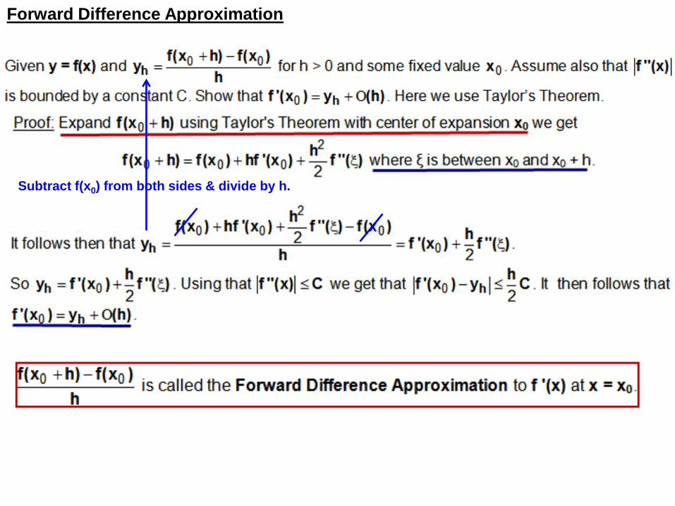
Forward Difference Approximation

Subtract f(x0) from both sides & divide by h.

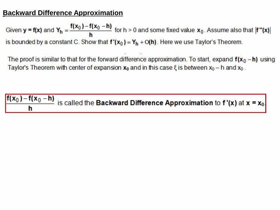
Backward Difference Approximation

A piece of theory we will use.

Discrete Average Value Theorem

Let f be in C([a,b]) and consider the sum where each point

xk is in [a, b], and the coefficients satisfy ak ≥ 0 , . Then there exists a

point η in [a,b] such that f(η) = S, i.e., .

Then by the Extreme Value Theorem there is an M in [a, b] so that fM = f(M) and

similarly there is an m in [a, b] so that fm = f(m). Hence f(m) ≤ S ≤ f(M).

Now apply the Intermediate Value Theorem so that there is an η in [a,b] so that

f(η) = S.

1

1n

kk

a

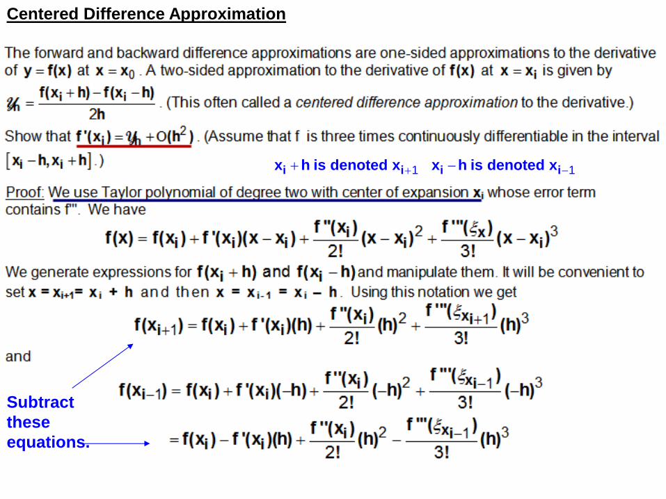
Centered Difference Approximation

Subtract

these

equations.

1 1i i i ix h is denoted x x h is denoted x

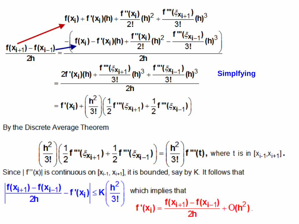
Simplfying

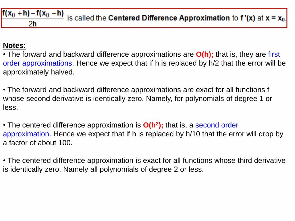
Notes:

• The forward and backward difference approximations are O(h); that is, they are first

order approximations. Hence we expect that if h is replaced by h/2 that the error will be

approximately halved.

• The forward and backward difference approximations are exact for all functions f

whose second derivative is identically zero. Namely, for polynomials of degree 1 or

less.

• The centered difference approximation is O(h2); that is, a second order

approximation. Hence we expect that if h is replaced by h/10 that the error will drop by

a factor of about 100.

• The centered difference approximation is exact for all functions whose third derivative

is identically zero. Namely all polynomials of degree 2 or less.

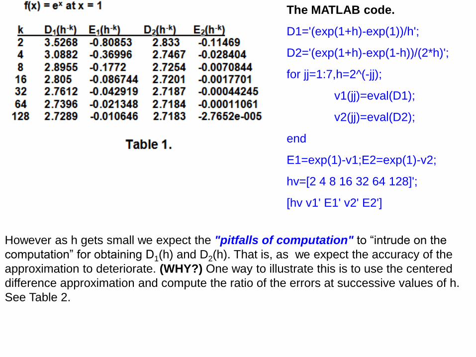
The MATLAB code.

D1='(exp(1+h)-exp(1))/h';

D2='(exp(1+h)-exp(1-h))/(2*h)';

for jj=1:7,h=2^(-jj);

v1(jj)=eval(D1);

v2(jj)=eval(D2);

end

E1=exp(1)-v1;E2=exp(1)-v2;

hv=[2 4 8 16 32 64 128]';

[hv v1' E1' v2' E2']

However as h gets small we expect the "pitfalls of computation" to “intrude on the

computation” for obtaining D1(h) and D2(h). That is, as we expect the accuracy of the

approximation to deteriorate. (WHY?) One way to illustrate this is to use the centered

difference approximation and compute the ratio of the errors at successive values of h.

See Table 2.

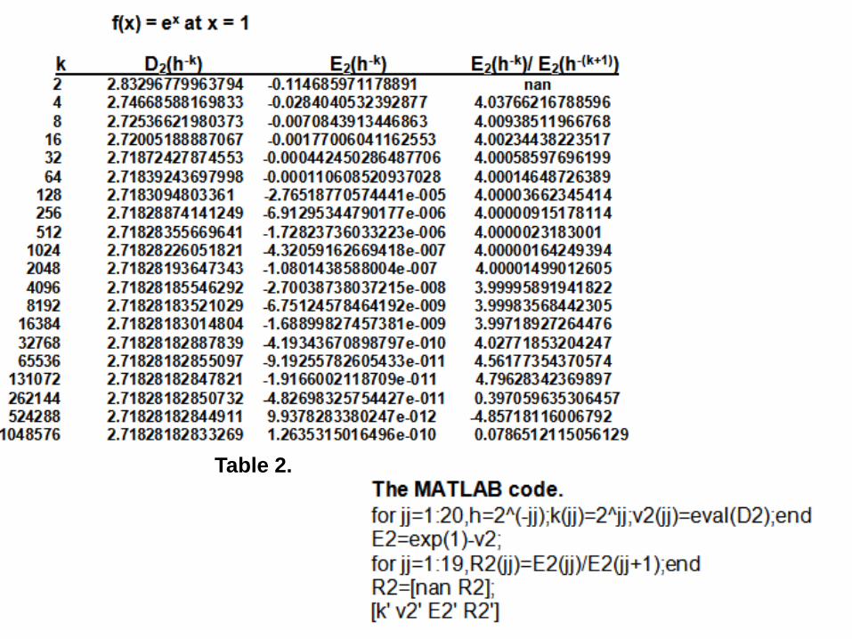
Table 2.

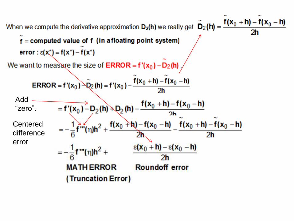
Add

“zero”.

Centered

difference

error

The total error in the centered difference approximation is due in part to

truncation error. If we assume that the round-off errors e(x0 ± h) are bounded

by some number ε > 0 and that the third derivative of f is bounded by a

number M > 0, then

To reduce the truncation error, h2M/6, we must reduce h. But a h is reduced,

the roundoff error ε/h grows. In practice, then, it is seldom advantageous to

let h be too small since roundoff error will dominate the calculations.

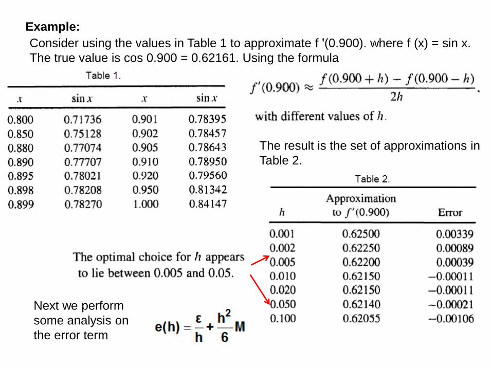
Example:

Consider using the values in Table 1 to approximate f ꞌ(0.900). where f (x) = sin x.

The true value is cos 0.900 = 0.62161. Using the formula

The result is the set of approximations in

Table 2.

Next we perform

some analysis on

the error term

The error term

We can use calculus to verify that a minimum for e occurs at , where

Since values of f are given to five decimal places, we will assume that the

round-off error is bounded by e = 0.000005. Therefore, the optimal choice of h

is approximately

which is consistent with the results in Table 2.

In practice, we cannot compute an optimal h to use in approximating the

derivative, since we have no knowledge of the third derivative of the function

when we only have a data set defining the function. But we must remain

aware that reducing the step size will not always improve the approximation.

We have considered only the round-off error problems that are presented by

the three point formula for centered differences, but similar difficulties occur

with all the differentiation formulas. The reason can be traced to the need to

divide by a power of h.

In the case of numerical differentiation, it is impossible to avoid the problem

entirely, although the higher-order methods reduce the difficulty.

Graphically the error in the centered

difference looks like

As approximation methods, numerical differentiation is unstable, since the small

values of h needed to reduce truncation error also cause the round-off error to grow.

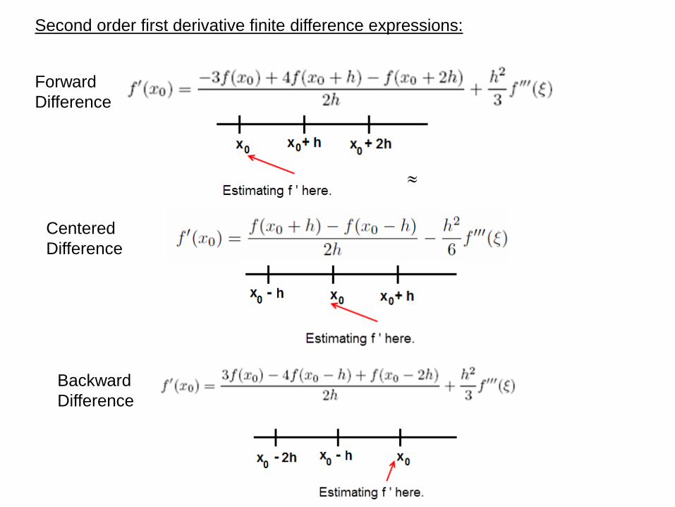
Second order first derivative finite difference expressions:

Forward

Difference

Centered

Difference

Backward

Difference

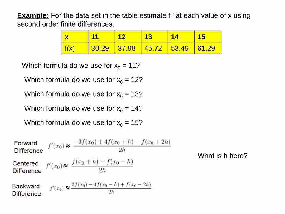
Example: For the data set in the table estimate f ꞌ at each value of x using

second order finite differences.

x 11 12 13 14 15

f(x) 30.29 37.98 45.72 53.49 61.29

Which formula do we use for x0 = 11?

Which formula do we use for x0 = 12?

Which formula do we use for x0 = 13?

Which formula do we use for x0 = 14?

Which formula do we use for x0 = 15?

What is h here?

x 11 12 13 14 15

f(x) 30.29 37.98 45.72 53.49 61.29

forward

backward

centered

x 11 12 13 14 15

f(x) 30.29 37.98 45.72 53.49 61.29

f ꞌ(x) ≈ 7.665 7.715 7.755 7.785 7.815

Let’s compare the approximate rates of change with the true values.

The original data was obtain from f(x) = -60 + 8x +11 exp(-x/7).

>> f=sym('-60+8*x+11*exp(-x/7)');

>> df=diff(f)

df = 8 - (11*exp(-x/7))/7

>> eval(vectorize(df))

ans = 7.6735 7.7170 7.7547 7.7873 7.8156

x 11 12 13 14 15

f(x) 30.29 37.98 45.72 53.49 61.29

f ꞌ(x) ≈ 7.665 7.715 7.755 7.785 7.815

f ꞌ(x) 7.6735 7.7170 7.7547 7.7873 7.8156