Sensor Studies

SUMMARY OF MICHIGAN MULTISPECTRAL

INVESTIGATIONS PROGRAM

by

Richard R. LegaultWillow Run Laboratories

The University of MichiganAnn Arbor, Michigan

INTRODUCTION

This paper is a summary of the NASA supported activities at TheUniversity of Michigan's Willow Run Laboratories in the area of multi-spectral remote sensing. The objectives of this program are to improveand extend the techniques for multispectral recognitions of remotelysensed objects. The program has two major areas of activity. The firstis a series of investigations directed in improving the techniques; thesecond is a series of programs with various users to extend the useful-ness of these techniques and to show their practical application. Inthis paper, I shall summarize the activities of the past year in thedevelopment of multispectral techniques. The paper following will discussthe exploitation of the techniques developed in previous years, as wellas those developed in this last year.

The primary thrust of last year's activities has been the developmentof techniques to extend spectral signatures in space and time. The funda-mental barrier to the multispectral signature extension has been variationsin the environment. These variations are differences, both spatially andtemporally, in atmospheric transmission, illumination of the scene, andbackscatter components. In previous years we pointed out that there arethree ways one may hope to obtain such signature extensions. The firstis by making suitable transformations on the remotely collected multi-spectral data; the intent of these transformations is to make the datainvariant despite variations in transmission, illumination and backscatter.The second possible method is to employ ancillary sensors in the datacollection platform which, in fact, do measure the illumination, trans-mission and backscatter. An example of such an ancillary sensor is thesun sensor now flown in the Michigan C47 aircraft. The third techniqueis to select in-scene references, which provide a calibration or referencesource in the scene that permit us to correct the data.

The second area of effort has been the development of data upon whichspectral signatures can be based. The data referred to here is laboratorydata of the spectral reflectance and transmission of various materials.In addition, models of various types of problems have been constructed and,as we shall show later, are exploited to investigate various problems inremote sensing. This effort has resulted in the compilation of data andmethods for retrieving this data for the remote sensing community as awhole.

400

SECTION 37

https://ntrs.nasa.gov/search.jsp?R=19720004637 2018-05-31T23:04:05+00:00Z

37-2

The third effort has been the development of techniques which showsome promise of enabling us to determine the composition of spatiallyunresolved scene elements. We shall treat the subject in fair detaillater.

The fourth area of effort has been an investigation of the problemsof multispectral data processing. Our attention has been directed towardspractical speeds for such computations. We shall treat this subject insome detail as it has been a matter of some discussion in past meetings.This discussion has centered around the relative merits of digital andanalog computation in the past. We will show that, in fact, both tech-niques have their place in an operational system.

Finally, some attention has been paid to problems of multispectralinstrumentation. We shall not discuss the work we have done in this areain this paper.

Twelve reports will be issued on the work of this past year. Duringthe course of the summary, I shall refer to these reports so that thoseinterested in more detail than we have time to present here can have therequired reference.

SIGNATURE EXTENSION

Spectral signatures are obtained today in the following manner. Theobjects to be recognized are identified in image form and from these areasthe statistics for defining the spectral signatures are obtained. Theproblem at present is that the signatures obtained in this fashion usuallydo not hold for areas very far distant from the original learning set orfor times very much different than the original collection time. A conse-quence of this is that a considerable amount of ground truth has to becollected in order to make effective use of spectral recognition techniques.Despite this rather obvious shortcoming, spectral recognition has playeda role and undoubtedly will continue to do so, but perfection of the tech-nique will require methods which allow us to extend the signature in bothspace and time. Equation (1) presents the rather unusual expression forthe signal in the ith spectral channel obtained by a multispectral remotesensor.

S(Xi, e) = [H(Xi)T(Ai, O)P(Xi, e) + b(Ai,e)]Ki (1)

401

37-3

where S(Xi,e) = signal from instrument

xi = spectral interval

0 = parameters of observation, direction, and distance

H(A i ) = irradiance (direct and diffuse sunlight)

r(Xie) = transmission

p(Xi,0) = material reflectance

b(XAi,) = backscatter

K. = instrument response1

The term that carries the information about the material in the expressionis of course the reflectance of the material, p(X ,0) and it is variationin this reflectance from one material to another Chat permits an identifi-cation. One is all too well aware, however, that we may expect variationsin the irradiance or illumination H(A), transmission or visibility (XA) andin the backscatter component b(I). These variations of illumination,transmission and backscatter are a primary source for the variation of theremotely sensed spectral signature and are a major contributor to the dilemmawe face today in terms of signature extension.

That illumination, transmission and backscatter should vary from onearea to another or from one time to another is not surprising, and consider-ing that our present method for processing the data is to accept thesevariations, it is again not surprising that we have difficulty in establish-ing spectral signatures that will hold for very large areas or for very longperiods of time.

One method for obtaining a spectral signature that is, in fact, invariantunder variations in these environmental factors of illumination, transmission,and backscatter, is the transformation of the remotely sensed spectral datato obtain a new set of values which are hopefully invariant. Last year, wereported on some of the ratioing or normalizing transformations and illustratedtheir success under certain circumstances. Tabulated below are some of themultispectral transformations that we have tried.

S(X 1 ,e) S(llle)

s(A2'9) "" S(x12,e)

S(X2 ,e) S(X12',)s(x 1

1,eeS(Xl,e ......a *Sxlle)

s.(X 2,e) - s(xl,e) S(A1 2,e) - S(ille

S(X, ) + S(18 6) ...... 'S( 8) + S(Xl 0)2' ~ ~ ~ ~,(12,8 (Xle

402

37-4

The reader is referred to Reference 1 to see some of the successes thatwere obtained. Now, these transformations essentially assume that we canignore the backscatter component. They further assume that the ratio ofillumination and transmission for two adjacent channels is essentiallya constant.

H(Ai)Tr(i,e)

H(Ai+l) j i+l, 0)

The above expression is a constant for all atmospheric conditions and forall wavelengths. These techniques have been partially successful. In ourview, the major failure of these techniques has been in their inability toadequately compensate for variations in the angles of observation.

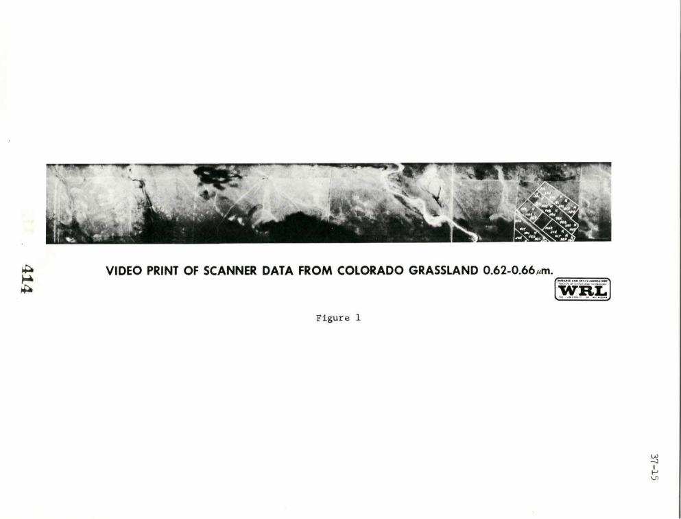
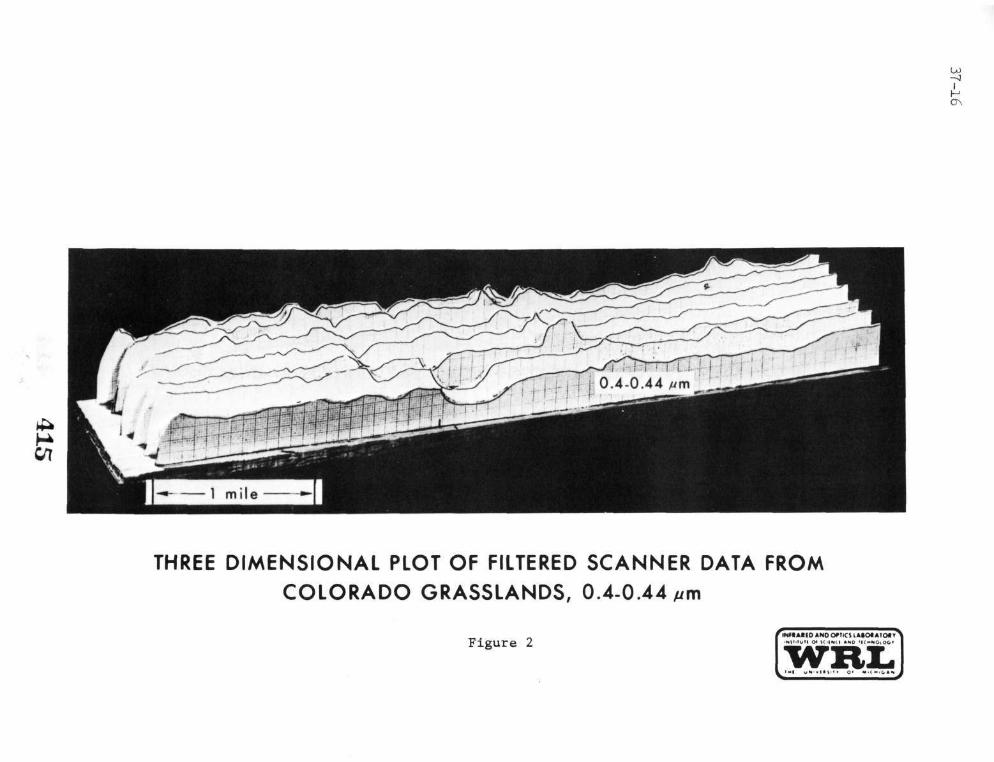
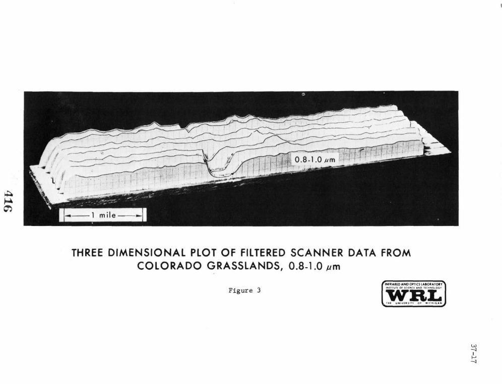
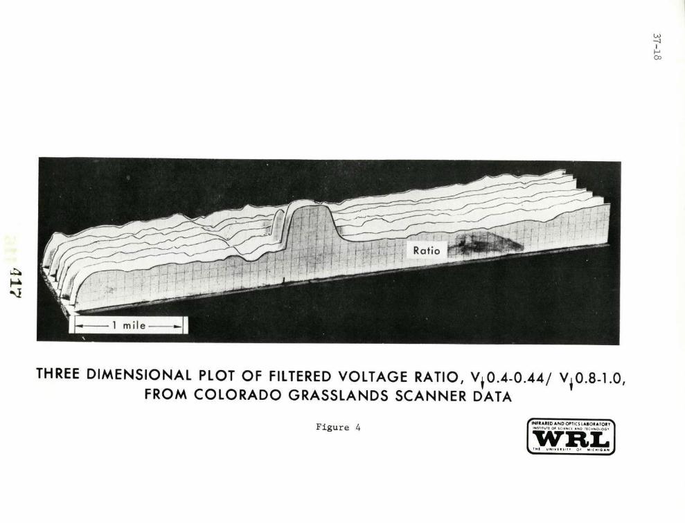
These angular effects are illustrated in Figures 1, 2 and 3. InFigure 1, we have a video print of scanner data of Colorado grassland.Figure 2 is a three dimensional representation of the signal amplitudefor a scanner strip of this area in the 0.4 to 0.44 pm regions; in Figure3 a similar strip of the same area is shown in the 0.8 to 1 pm band.The reader can get a rough impression of the general slope or angulardependence by looking at the latter two figures. It should be apparentthat the angular effects are, in fact, wavelength dependent by comparingthe two figures. The very prominent dip in both of these figures is acloud shadow,and in Figure 4 we will show a rather interesting methodfor detecting cloud shadows in the imagery.

In Figures 2 and 3, the horizontal dimension represents the flightpath and the vertical dimension represents the scan dimension and is denotedin subsequent descriptions of the scan angle variations. If one looksclosely at this data, one sees that if we average over local variations, afairly well defined scan angle variation is sensible. This correctionfactor for scan angle is essentially obtained by averaging in the flightpath dimension for a fixed scan angle and fixed spectral interval. Thisaveraging process is represented in equation (2) below:

1 Tf(Xi,8) = S(Xi,O,T)dT (2)

where T = flight path dimension

8 = scan angle

The primary question, of course, is the interval over which suchaveraging should take place; in other words, how long a path length Tshould we take for finally determining the value of f(X.) for a fixedvalue of 0. The inverse of the correction function f(i,08) is then usedto correct the remotely sensed data for angular effects. This techniqueis fairly obviously a combination of the transformed techniques discussed

403

37-5

earlier as well as the employment of in-scene references. In the particularscene in which this has been exploited so far, the various different elementshave been randomly scattered with respect to the scan angle. Thus, we havea fairly unbiased estimate of the angular effects exploiting this averaging.Reference 1 covers in more detail this technique and some of the other workon transformation techniques that we have done during the past year, andreference 2 discusses the application of that technique to some actual data.The second paper will cover in more detail the results of this exploitationof the technique.

Figure 4 is a ratio of the 0.4 to 0.44 pm bands to the 0.8 to 1 pmband. It is rather interesting to note that the cloud shadow becomes veryobvious in this ratio presentation. The reason I think is fairly clear,that the cloud shadow is relatively darker in the 0.8 to 1 pm band thanit is in the 0.4 to 0.44 pm band, the difference largely due to the factthat the short wavelength 0.4 to 0.44 pm band is primarily direct sunlight.The identification of cloud shadows and the subsequent correction of thedata for cloud shadows detected in this manner is another way to extendthe spectral signatures.

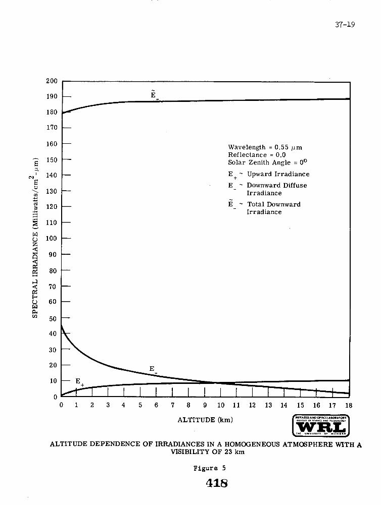
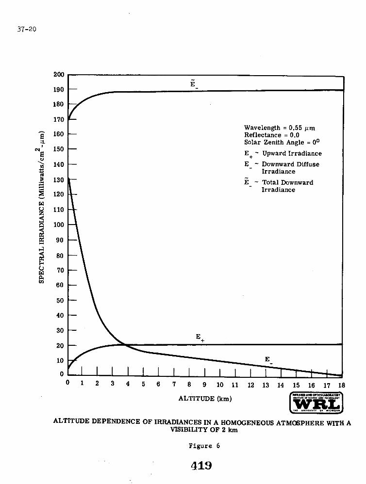
A second method for extending the spectral signatures is to employancillary sensors in the remote sensor platform to measure illumination,transmission and backscatter. At the present time, the Michigan C47 air-craft carries a sun sensor which measures the total downward irradiance atthe aperture of the sun sensor. We have found that normalization of theremotely sensed multispectral data by the sun sensor data collected in eachchannel during the dead time of the scan has enabled us to extend the spectralsignatures significantly. However, the simple normalization techniques havenot accomplished all that we might desire. Consequently, we have initiatedinvestigations into the calculation of the signals received by various typesof sun sensors and the relationship to the backscatter, transmission andground irradiance or illumination values. Figures 5 and 6 are the rEultsof some of these calculations for albedos at the ground plane of 0.Figure 5 shows computations for visibility range of 23 km and Figure 6 forvisibility range of 2 km, a quite significant difference in the atmosphericconditions.

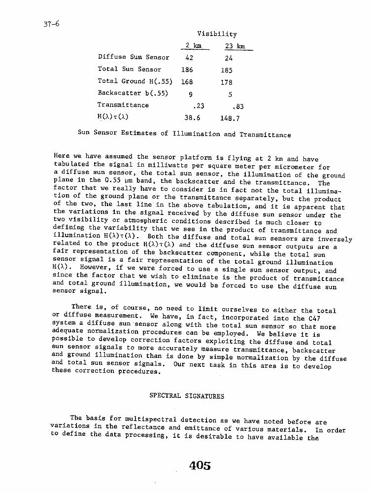
The first impression that one receives in looking at this data is thefact that the total downward radiation which is currently being measured byour sun sensor is not nearly as sensitive to variations in the atmosphericconditions as is the diffuse downward component. This is hardly surprisingsince the diffuse component as measured from the aircraft platform (providedit is well within the atmosphere) should, in fact, be a fair measure of theatmospheric conditions. The real test of the importance of this is seenin the following tabulation.

404

37-6Visibility

2 km 23 km

Diffuse Sun Sensor 42 24

Total Sun Sensor 186 185

Total Ground H(.55) 168 178

Backscatter b(.55) 9 5

Transmittance .23 .83

HXA) T() 38.6 148.7

Sun Sensor Estimates of Illumination and Transmittance

Here we have assumed the sensor platform is flying at 2 km and havetabulated the signal in milliwatts per square meter per micrometer fora diffuse sun sensor, the total sun sensor, the illumination of the groundplane in the 0.55 pm band, the backscatter and the transmittance. Thefactor that we really have to consider is in fact not the total illumina-tion of the ground plane or the transmittance separately, but the productof the two, the last line in the above tabulation, and it is apparent thatthe variations in the signal received by the diffuse sun sensor under thetwo visibility or atmospheric conditions described is much closer todefining the variability that we see in the product of transmittance andillumination H(X)T(X). Both the diffuse and total sun sensors are inverselyrelated to the product H(C)T(X) and the diffuse sun sensor outputs are afair representation of the backscatter component, while the total sunsensor signal is a fair representation of the total ground illuminationH(X). However, if we were forced to use a single sun sensor output, andsince the factor that we wish to eliminate is the product of transmittanceand total ground illumination, we would be forced to use the diffuse sunsensor signal.

There is, of course, no need to limit ourselves to either the totalor diffuse measurement. We have, in fact, incorporated into the C47system a diffuse sun sensor along with the total sun sensor so that moreadequate normalization procedures can be employed. We believe it ispossible to develop correction factors exploiting the diffuse and totalsun sensor signals to more accurately measure transmittance, backscatterand ground illumination than is done by simple normalization by the diffuseand total sun sensor signals. Our next task in this area is to developthese correction procedures.

SPECTRAL SIGNATURES

The basis for multispectral detection as we have noted before arevariations in the reflectance and emittance of various materials. In orderto define the data processing, it is desirable to have available the

405

37-7

reflectivities and emissivities of various materials so that the potentialfalse alarms as well as detection probabilities may be calculated beforeexpensive operational tests of the detection procedure are made, To thisend, we have compiled the available spectral reflectance and emittancedata; this data compilation is reported in reference 3. The spectralsignature data has, in addition, been digitized and retrieval programshave been generated. This retrieval and analysis program is described inreference 4. The digitized data are also available to the remote sensingcommunity from either Houston or The University of Michigan. The availablespectral data are far from complete; the data gaps are identified inreference 5. It is our hope that the remote sensing community will colla-borate with us in filling these gaps and we hope that this document willbe of use to other organizations in planning their measurement programs.

We have in addition exploited this data to some newer applicationsfor remote sensing techniques. As most of you are aware today, our opera-tions are limited to the 0.32 to 1 pm region. In the very near futurewe shall have common aperture multispectral sensors from 0.32 to 14 pmand it seems very obvious that we should start considering the use ofmultispectral thermal or infrared data. Figure 7 is a composite plotof the emission spectra of various silicon dioxide based rocks. It iswell known that the emissivity dip in the 9 to 10 pm region is due to thereststrahlen of silicon dioxide. The minimum of this reststrahlen dipfor acidic rocks occurs at a shorter wavelength (roughly 9.4 pm) thandoes the minimum for ultra basic rocks (roughly 10.2 pm). It should thennot be surprising that one might attempt to define the acidity of variousrock types on the basis of multispectral data collected in the 9 to 11 pmregion. Some manipulation of these data convinced us of the potentialof this technique.

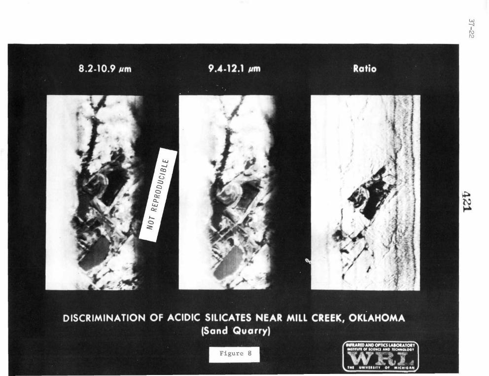
A recently developed laminar detector was made available to us. Thetop layer of this detector was sensitive in the 8.2 to 10.9 pm range andthe bottom detector was sensitive in the 9.4 to 12.3 pm range. A briefglance convinces one that there is some hope that by taking the ratio ofthese two bands, the acidity of the rock type might be determined. Whilethe spectral bands encompassed by this detector are not optimal for thistask by any stretch of the imagination, it is the first common aperturemultispectral data available to us in the 8 to 14 pm band.

In Figure 8 we show the images collected in the two bands respectivelyas well as the ratio. If the ratio of the 8.2 to 10 pm channel to the9.4 to 12.1 pm channel is small, we would tend to say that acidic rockis present. In the ratio image of Figure 8, we see fairly dim areasaround a silicate quartz sand quarry in Mill Creek, Arizona. In the twoimages separately, a body of water is noted in the lower central portionof the image. In the ratio image a dark outline for these areas indicatesthe sand shores of this body of water. Subsequently, Dr. Kenneth Watsonof USGS and his colleagues have walked this area and identified all the

406

37-8

dark portions of this particular scene as being high. acidic, silicon-dioxide-based rocks. While they have not investigated all the otherportions of this scene, they have not found any other silicon-dioxide-based rocks that were not detected by this ratio technique. This workis reported in reference 6.

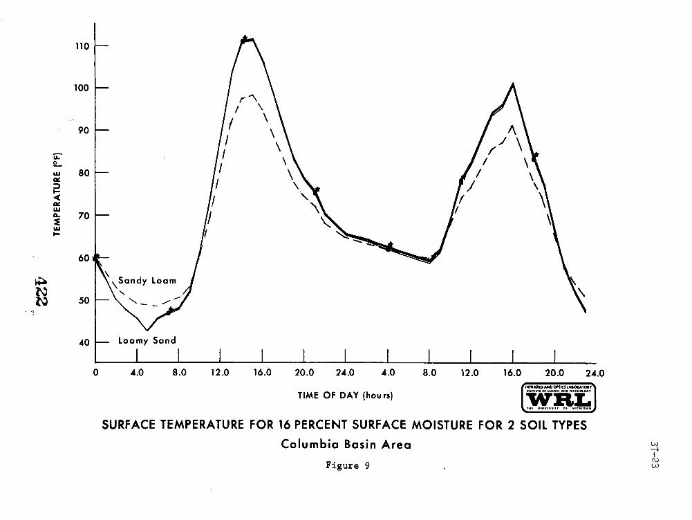
The spectral signatures work in the past year has also included somemodeling of the radiation characteristics for various phenomena. One ofthe tasks undertaken was an attempt to determine whether ground watercould be detected in thermal imagery. This work was in support of somedata interpretation for the Columbia Basin area. There was some indicationthat thermal patterns in the scene were associated with varying depths ofwater table in this particular area. Consequently, calculations were madeto determine whether the temperature as measured at the surface could beused as an indicator of the water table. The environmental conditions,relative humidity, temperature, time of the year and wind velocities forthe period of data collection were used in these calculations. We used aone dimensional thermal model which allows us to assume various types ofmaterials in layered structures.

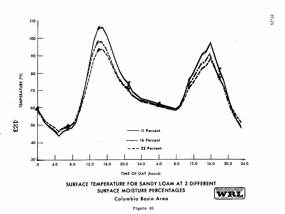
In Figure 9 is plotted the diurnal cycle for temperature variationsfor two soil types. It should be noted that at certain times of the day,the differences of soil types do in fact produce different temperatureswhich would be detectable by an IR scanner. In Figure 10, differentmoisture contents for a single soil type were assumed and once again foroptimal times of day detectable temperature differences are present.

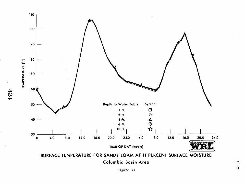
In Figure 11, we considered a structure for the terrain with thewater table at varying depths but with identical surface moistures andsoil types. It is apparent that no detectable temperature differencesfor the environmental conditions postulated (in this particular example,they were in the late fall) are detectable. If underground water is goingto be detected, it is likely that it will be by one of three means -either differences in vegetation types present at the surface whereunderground water is present, differences in soil moisture (which isvery likely to occur), or differences in soil types probably relatedto permeability of the soil. While there still remains some hope fordetection of underground water based upon remotely sensed infrared radia-tion, more work on the mechanism of such detection seems warranted at thistime. It is also clear that both the time of day for this detection pro-cess and time of year will play an essential role.

DETECTION OF SPATIALLY UNRESOLVED OBJECTS

Much has been said to date of the problems associated with the limitedspatial resolution capabilities of the first generation satellite-borneremote sensors. These remote sensors have concentrated on spectral coverage

407

37-9

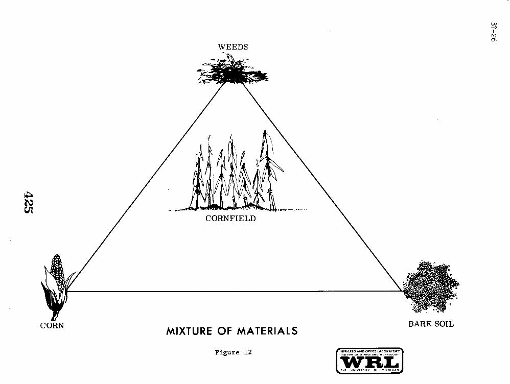
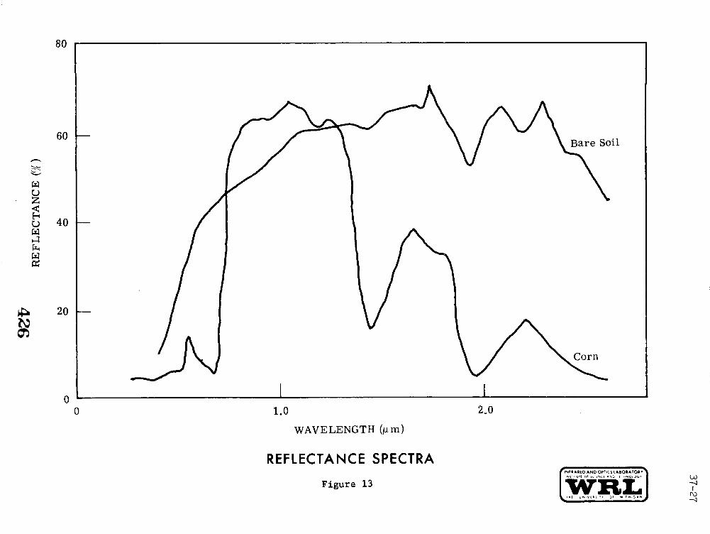
rather than spatial coverage. That this concentration is warranted ispartially demonstrated in the following work that was done during thelast year. At first glance, it would seem impossible to identify objectsthat are spatially unresolved. This is certainly true if we are consider-ing single spectral channel systems. However, the ability to measure thespectral distribution of radiance does offer us the possibility to resolvethe elements within a resolution element -- in other words, the capabilityof identifying spatially unresolved objects. One example is the percentground cover of an agricultural crop which is indicative of stage of growthand vigor. In Figure 12, we have such a classical problem, viz. thedetection of the amount of weeds and bare soil in a corn field. Now letus consider this particular corn field as being a composite of corn plantreflectance spectra, the reflectance spectra of weeds and the reflectancespectra of bare soil. There is a certain percentage of each one of thesepure types of materials in an individual resolution element. Very fewsensors at almost any aircraft altitude are able to tell us very preciselywhat these percentages are. However, if we consider the multispectralsignature of each individual type of materials (weeds, corn plant and soil)as vertices of a convex mixture, then the particular field we are lookingat contains percentages of each. of these types. In Figure 13, we have thereflectance spectra of bare soil and corn. These are pure spectral signa-tures of each of the materials. Now suppose a particular resolutionelement contains equal amounts of corn and bare soil while another resolu-tion element contains 20% corn and 80% bare soil. We expect to seedifferences in the reflectance spectra for the various resolution elementsand, in fact, we do as a scene in Figure 14. We are in fact able to takethis composite spectrum and determine the percent of various elementsthat are within the resolution element.

A model for this detection is follows:

MODEL

Signature of Type i Material is GaussianDistribution with Mean A

iand Covariance

Matrix Mi . If Proportion of Type i Materialin Mixture is Xi, Signature of Mixture HasMean A and Covariance Matrix M Given by:

x x

Ax =L.XiA i

M = XiMi

i

408

37-10

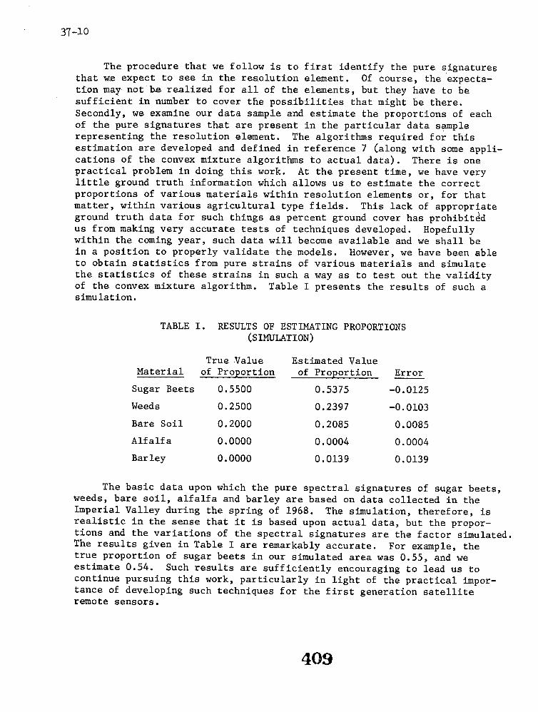
The procedure that we follow is to first identify the pure signaturesthat we expect to see in the resolution element. Of course, the expecta-tion may not ba realized for all of the elements, but they have to besufficient in number to cover the possibilities that might be there.Secondly, we examine our data sample and estimate the proportions of eachof the pure signatures that are present in the particular data samplerepresenting the resolution element. The algorithms required for thisestimation are developed and defined in reference 7 (along with some appli-cations of the convex mixture algorithms to actual data). There is onepractical problem in doing this work. At the present time, we have verylittle ground truth information which allows us to estimate the correctproportions of various materials within resolution elements or, for thatmatter, within various agricultural type fields. This lack of appropriateground truth data for such things as percent ground cover has prohibitedus from making very accurate tests of techniques developed. Hopefullywithin the coming year, such data will become available and we shall bein a position to properly validate the models. However, we have been ableto obtain statistics from pure strains of various materials and simulatethe statistics of these strains in such a way as to test out the validityof the convex mixture algorithm. Table I presents the results of such asimulation.

TABLE I. RESULTS OF ESTIMATING PROPORTIONS(SIMULATION)

True Value Estimated ValueMaterial of Proportion of Proportion Error

Sugar Beets 0.5500 0.5375 -0.0125

Weeds 0.2500 0.2397 -0.0103

Bare Soil 0.2000 0.2085 0.0085

Alfalfa 0.0000 0.0004 0.0004

Barley 0.0000 0.0139 0.0139

The basic data upon which the pure spectral signatures of sugar beets,weeds, bare soil, alfalfa and barley are based on data collected in theImperial Valley during the spring of 1968. The simulation, therefore, isrealistic in the sense that it is based upon actual data, but the propor-tions and the variations of the spectral signatures are the factor simulated.The results given in Table I are remarkably accurate. For example, thetrue proportion of sugar beets in our simulated area was 0.55, and weestimate 0.54. Such results are sufficiently encouraging to lead us tocontinue pursuing this work, particularly in light of the practical impor-tance of developing such techniques for the first generation satelliteremote sensors.

409

37-11

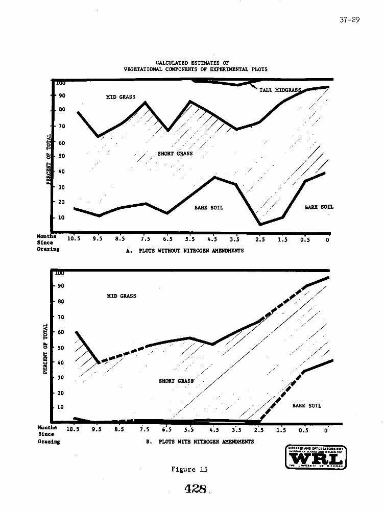
The only practical application of this technique made to date hasbeen over a Colorado grasslands area where various nitrogen fertilizertreatments were applied. While once again we had inadequate ground truthto determine the percentages of tall, mid-length and short grasses on thevarious plots investigated, it was possible to at least quantitativelydetermine whether the algorithm was working properly. In Figure 1, wehave a panchromatic image of the Colorado grassland area where the nitrogentreatments were applied. The treatments were applied at various times sothat data was available on the height of the grass from the time of treat-ment. As we can see in Figure 15, the algorithm predicts more tall grassfor the nitrogen treated plots than for plots receiving no treatments andthat the rate of growth of the grass is greater for the nitrogen treatedplots, as we might expect. In this particular case, we have specifiedpercentages of the three grass heights that were involved. The best thatwe can say is that the results agree with what our intuition would be. Aswe have said before, there is no ground truth to support the results ofthese estimations. Various problems with the computational algorithmshave been identified and work is currently going on to correct them. Thetechnique will be exploited with more airborne data during the coming year.

DATA PROCESSING

Multispectral processing of remotely sensed data has proven effectivein many applications related to earth resources studies. However, theseapplications usually require timely processing of large quantities of dataand today this processing is several orders of magnitude beyond our capa-bilities. For example, if the U.S. and its coastal waters were overflowntwice a year with presently planned equipment, the data collected wouldrequire a conventionally organized digital computer with a cycle time of10-10 seconds to keep pace with the data collection rates. This cycle timeis a factor of 104 faster than that obtainable with presently availabledigital computers. Alternative methods of computations are available. Aparallel-channel, hard-wired analog computer system at The University ofMichigan (SPARC) does in fact meet this data rate. However, there aredrawbacks with this type of system. The set up of such an analog computeris extremely slow and its versatility is somewhat limited, whereas thedigital computer is a much more versatile device. It seems, then, fairlyclear that the type of operational data processing system that we willultimately be led to combines the best features - program ability primarilyof the digital computer, and the high throughput calculation rate of hard-wired, parallel-channel analog facilities.

During the past year, we have investigated the possible design alterna-tives for such a hybrid multispectral data processing facility. The resultsof these investigations are given in detail in references 8 and 9. Essen-tially these investigations began by considering some of the limitations

410

37-12

of the current analog systems. The major problems with. the current analog

systems are the time involved in setting up the problem for computationand the difficulty in optimizing the recognition procedure. It became

fairly clear that an improved system should utilize a digital facility in

the problem set up and the process optimization, and rely on the parallelismof the analog portion of the system for the bulk computation. Thus, we

have a fairly standard hybrid where the digital computation system acts asa controller for the analog processor which does the high speed parallelchannel computation.

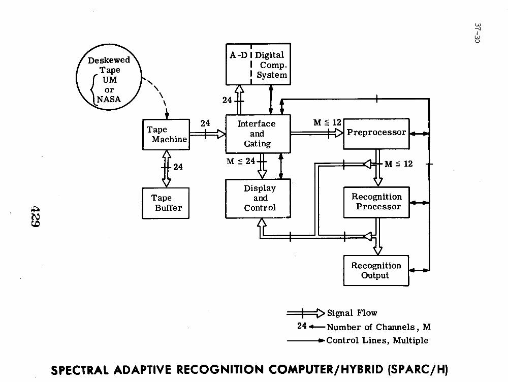
In Figure 16, we have a component diagram for such a system which

indicates the various types of units that are involved. We have data inputs

and data primarily from magnetic tape, tape buffer storages, interfaces

between both display and digital computer for the analog processor, pre-processor and the analog recognition processor. The recognition output is

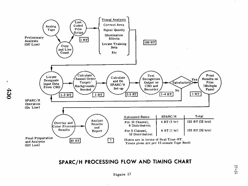
then interrogated by the digital system for determining whether it isoperating according to plan. In Figure 17, we see the various functionsthat are performed and some estimate in terms of factors of real time for

these various functions. The proposed hybrid system gives an effectivereduction of a factor of 32 in the time for processing multispectral data.The type of equipment proposed here is, of course, prototype and there is

little doubt that with more engineering work that hybrid facilities could,in fact, be designed to meet real time.

INSTRUMENTATION

During the past year, three small studies of multispectral instrumen-tation have been performed. The results of these investigations are givenin references 10, 11 and 12. We shall not discuss these reports in anydetail. Very briefly, we considered the utilization of detectors in linescanners, some optical transfer techniques for multispectral orbitalscanners, and some problems of calibrating multispectral scanners. Theseproblems had arisen during the design and fabrication of the 24-channelmultispectral scanner for aircraft use and the 10-channel Skylab sensor.These studies were an integral part of the engineering support we furnishedNASA, Houston during the fabrication of the 24-channel and Skylab sensors.

CONCLUSIONS

I should like to be able to report that our work on the spatial andtemporal extension of multispectral signature had been completed. I cannot.A complicated multispectral recognition problem that required 219 learningsets last year can now be done with 13 learning sets. Signatures that were

411

37-13

valid for 30 miles last year have been extended for 129 miles usingtransformation and sun sensor data. But there are still cases whereour techniques will not work. We have sorted out most of the problemsof signature extension and expect next year to be able to define thelimits of signature extension and how the extension should be attained.

Spectral reflectance and emittance data are now available to theremote sensing community. This data can be used to define the approachto many multispectral remote sensing problems. All too often multi-spectral recognition is based on spectral differences which appear ina set of remotely sensed data without our being able to explain whysuch differences should be present. Consequently, we are unable tostate with any certainty whether the recognition experiment can berepeated. An explanation of the observed differences based on theoptical properties of the materials gives us some confidence of therecognition experiment's repeatability. We hope that the successfuluse of signature data reported will persuade the remote sensing investi-gators to make more extensive use of such data.

The most exciting new development is the possibility of recognizingspatially unresolved scene elements using multispectral data. Thesetechniques are in their infancy but show considerable promise. A newfactor must now be considered when defining required spatial resolutions.If spatially unresolved elements can be identified in some cases usingmultispectral data, we should have a new look at the remote sensingproblems requiring high spatial resolution to determine whether or notthey can be solved with the new multispectral recognition techniques forunresolved spatial elements.

412

37-14

REFERENCES

1. STUDIES OF SPECTRAL DISCRIMINATION, W. A. Malila, R. Turner,R. Crane, C. Omarzu, Report No. 3165-22-T, in publication.

2. INVESTIGATIONS RELATED TO MULTISPECTRAL IMAGING SYSTEMS FORREMOTE SENSING, J. Erickson, Report No. 3165-17-P, in publication.

3. THE NASA EARTH RESOURCES SPECTRAL INFORMATION SYSTEM: A DATACOMPILATION, V. Leeman, et.al., Report No. 3165-24-T, inpublication.

4. EXPANDED RETRIEVAL ANALYSIS SYSTEM FOR THE NASA EARTH RESOURCESSPECTRAL INFORMATION SYSTEM, V. Leeman, et.al., Report No.3165-22-T, in publication.

5. DATA GAPS IN THE NASA EARTH RESOURCES SPECTRAL INFORMATION SYSTEM,R. Vincent, Report No. 3165-25-T, in publication.

6. REMOTE SENSING DATA ANALYSIS PROJECTS ASSOCIATED WITH THE NASAEARTH RESOURCES SPECTRAL INFORMATION SYSTEM, R. Vincent, et.al.,Report No. 3165-26-T, in publication.

7. INVESTIGATIONS OF MULTISPECTRAL SENSING OF CROPS, R. Nalepka, et.al.,Report No. 3165-30-T, in publication.

8. A PROTOTYPE MULTISPECTRAL PROCESSOR WITH HIGH THROUGHPUT CAPABILITY,F. Kriegler, R. Marshall, Report No. 3165-23-T, in publication.

9. DATA PROCESSING DISPLAYS OF MULTISPECTRAL DATA, F. Kriegler,R. Marshall, Report No. 3165-28-T, in publication.

10. DETECTOR UTILIZATION IN LINE SCANNERS, Leo Larsen, Report No.3165-29-T, in publication.

11. CALIBRATION OF MULTISPECTRAL SCANNERS, J. Braithwaite, Report No.3165-27-L, in publication.

12. INVESTIGATION OF SHALLOW WATER FEATURES, F. Polcyn, et.al.,Report No. 3165-31-T, in publication.

413U

' "' "•W' ' *W. "**"'"*

£> K ^

VIDEO PRINT OF SCANNER DATA FROM COLORADO GRASSLAND 0.62-0

Figure 1

THREE DIMENSIONAL PLOT OF FILTERED SCANNER DATA COLORADO GRASSLANDS, 0.4-0.44 Mm

Figure 2

CT5

THREE DIMENSIONAL PLOT OF FILTERED SCANNER DATA F COLORADO GRASSLANDS, 0.8-1.0//m

Figure 3

THREE DIMENSIONAL PLOT OF FILTERED VOLTAGE RATIO, V^O.4-0. FROM COLORADO GRASSLANDS SCANNER DATA

Figure 4

37-19

E~~~~----- - - -

Wavelength = 0.55 ilmReflectance = 0.0Solar Zenith Angle = 00

E

E ~

E

Upward Irradiance

Downward DiffuseIrradiance

- Total DownwardIrradiance

I I I I I I I I 0 1 2 3 4 5 6 7 8 9 10 11 12 13 14 15 16 17 18

ALTITUDE (km)

ALTITUDE DEPENDENCE OF IRRADIANCES IN A HOMOGENEOUS ATMOSPHERE WITH AVISIBILITY OF 23 km

Figure 5

418

200

190

180

170

160

150

140

130

120

110

100

90

80

70

60

50

I-

C)

._

C.

Pc

40

30

20

10

0 I- E.

Wavelength = 0.55 /umReflectance = 0.0Solar Zenith Angle = 00

E+ - Upward IrradianceE - Downward Diffuse

Irradiance

E - Total DownwardIrradiance

E+ I

EI-LLLLL-

0 1 2 3 4 5 6 7 8 9 10 11 12 13 14 15 16 17 18

ALTITUDE (km) [i1ALTITUDE DEPENDENCE OF IRRADIANCES IN A HOMOGENEOUS ATMOSPHERE WITH A

VISIBILITY OF 2 km

Figure 6

419

37-20

I200

190

180

170

j 160::L

c4 150

U*W- 140

.3 130-: 120

i 110

100

5 90

g 80

cU 70

60

50

40

30

20

10

0 i I Ih. !L.

700 cm- 'I ! I

- Tektite--Dacite ACID ROCKSI/ Granite

- Pumice

- Trochyte

Garnetiferous Gabbro

Augite DioriteBASIC ROCK

Diabose

BasaltPlagioclase Basalt

ROCKS

S

a 4

ULTRABASIC ROCKS

I I I I I I

8 9 10 11 12 13 /

Figure 7

1300 1100 900

37-21

()

U)

l-J

U)Q

r0

zZ

i0.1

T

(ofter R. Lyon)

II I I . . . . . .lr I I I l ,

I

-- I

420

8.2-10.9 urn 9.4-12.1 m Ratio

DISCRIMINATION OF ACIDIC SILICATES NEAR MILL CREEK, OKLAH (Sand Quarry)

rd<.t\\,1\<:i Mfmvn of KII " " • — " - - ~ -f^i 1MI U W V I I H

|//

Sandy Loam

0 4.0 8.0 12.0 16.0 20.0 24.0 4.0

TIME OF DAY (hours)

SURFACE TEMPERATURE FOR 16 PERCENT SURFACEColumbia Basin Area

Figure 9

8.0 12.0 16.0 '20.0 24.0INFS CIARED AND I T ECS IATOICY

MOISTURE FOR 2 SOIL TYPES

INJ

oZU-

UJ

I--

C-

I-

110

100

90

80

70

60

50

40

I /r/

L)

IT\)

11 Percent

--- 16 Percent

--- 22 Percent

8.0 12.0 16.0 20.0 24.0 4.0 8.0 12.0 16.0

TIME OF DAY (hours)

SURFACE TEMPERATURE FOR SANDY LOAM AT 3 DIFFERENTSURFACE MOISTURE PERCENTAGES l

Columbia Basin Area

Figure 10

20.0 24.0

4IIAED AND O~TICS 1T1J0

,........ -- l-. Ot^."

110

100

90

80

70

50

2.-

LUa-

UP

Co

40

300 4.0

Depth to Water Table

1 Ft.2 Ft.

Symbol

0O

4 Ft.6 Ft.

0 4.0 8.0 12.0 16.0 20.0 24.0 4.0 8.0

TIME OF DAY (hours)

12.0 16.0 20.0 24.0

T _S LAMAO

SURFACE TEMPERATURE FOR SANDY LOAM AT 11 PERCENT SURFACE MOISTURE

Columbia Basin Area

Figure 11

110

100

90

uof

a.'U

I-1r-

80

70

60

50

40

30

o1rN

WEEDS

CORNFIELD

CORN MIXTURE OF MATERIALS BARE SOILMIXTURE OF MATERIALS

Figure 12 INFRARED AND OPTICS LABORAORY

_Wl E NIVILT OF ICIGN

A4Nn

1.0 2.0

WAVELENGTH (I-m)

REFLECTANCE SPECTRAINFRARE D AOOPICS lABOgA ]OY

--rl.ut Of Si ICI .s. 1. ...o_

l,,rf .?Figure 13

wUZ

H<F4

c,.)

5.144

w:

80

60

40

20

00

20"i, Corn80"'/, Bare Soil

/ \ 1~"--

50";, Corn50',/ Bare Soil

WAVELENGTH (jim)

REFLECTANCE SPECTRA OF MIXTURES

INFRARED AND OPTICS LABORATORYW-IjT H I. u .NO ICI-OLOG,

Figure 14

80

60 -

W

C-0-

v

Uz

U<

_: 40 - //

20

1-4Nf%j

\

/,

1.0 2.0

37-29

CALCULATED ESTIMATES OFVEGETATIONAL COMPONENTS OF EXPERIMENTAL PLOTS

- TALLMID GRASS

/~~~~:/J S / G /'/

'"' A./' ''/

, / .SHORT GRASS ,/' "/ "' '"

BARE SOIL BARE SOIL

10.5 9.5 8.5 7i .5 6.5 5.5 4.5 3.5

A. PLOTS WITHOUT NITROGEN AMENDMENTS

2.5 1.5 0.5 0

7.5 6.5 5.5 4.5 3.5 2

B. PLOTS WITH NITROGEN AMENDMENTS

Figure 15

428 .

4

C

D&I

0

iuo

90

80

70

60

50

40

30

20

10

Month L

SinceCrazing

6

D45'

21

14

MonthsSinceGrazing

INFRARED AND OPTICS LAIIt ATO

w1 # UI VI$1 Mf 'IcH. 0I j

I I I w1

p

L

eskewedTapeUM N

or\NASA Ii

4 24Tape

Machine

24

TapeBuffer

411

M - 12aIr %

i==> Signal Flow24 4-Number of Channels, M

-- o Control Lines, Multiple

SPECTRAL ADAPTIVE RECOGNITION COMPUTER/HYBRID (SPARC/H)

A -D I DigitalI Comp.I System

o.-

O

Interfaceand

GatingPreprocessor

M < 24

Displayand

ControlI. .

-M -< 12

RecognitionProcessor

RecognitionOutput

I i :

It 1L

IIli I

"'t4

I .A

PreliminaryAnalysis(Off Line)

(SPARC/HOperation(On Line)

Visual Analysis

Correct Area

Signal Quality

IlluminationEffects

Locate TrainingSets

Etc

Estimated Rates:

For 12 Channel,6 Distribution:

Final Preparationand Analysis(Off Line)

For 6 Channel,12 Distribution:

o20 RT| E3

SPARC/H

4 RT (1 hr)

4 RT (1 hr)

Total

125 RT (32 hrs)

125 RT (32 hrs)

(Rates are in terms of Real Time-RT.Times given are per 15 minute Tape Reel)

SPARC/H PROCESSING FLOW AND TIMING CHART

Figure 17

100 RT

.w-!

HO