Today: Section 12.2, Lesson 3: What can go wrong with hypothesis testing Section 12.4: Hypothesis tests for difference in two proportions ANNOUNCEMENTS: • No discussion today. • Check your grades on eee and notify me if any of them are incorrect. • Quiz #7 begins Wed after class and ends Friday. • Quiz #8 begins Wed before Thanksgiving and ends on Monday after

Thanksgiving. That is the last quiz. • Jason Kramer will give the lecture this Friday. HOMEWORK (due Fri, Nov 19): Chapter 12: #62, 83, 101

REVIEW OF HYPOTHESIS TEST FOR ONE PROPORTION ONE-SIDED TEST, WITH PICTURE H0: p = p0 versus Ha: p > p0

Reject H0 if p-value < .05. For what values of z does that happen? Notation: level of significance = α (alpha, usually .05) p-value < .05 corresponds with z > 1.645

Value of test statistic1.645

0.05

0

Normal, Mean=0, StDev=1

Reject null hypothesis

Do not reject null hypothesis

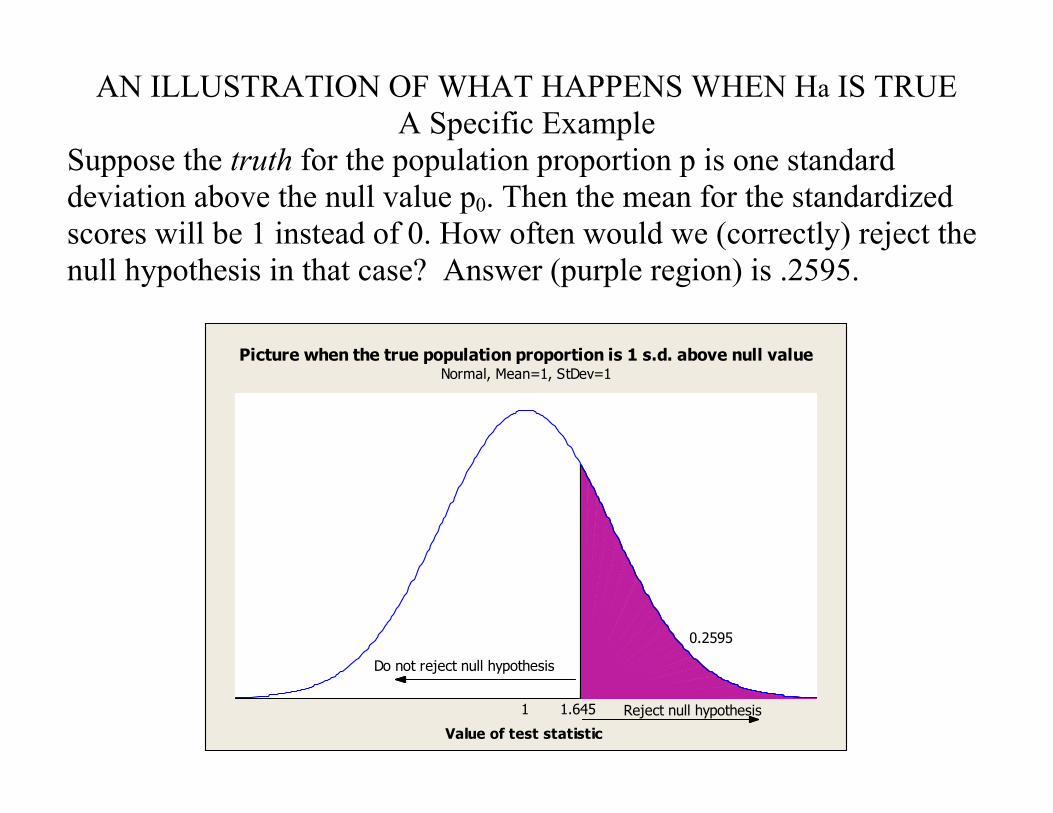
AN ILLUSTRATION OF WHAT HAPPENS WHEN Ha IS TRUE A Specific Example

Suppose the truth for the population proportion p is one standard deviation above the null value p0. Then the mean for the standardized scores will be 1 instead of 0. How often would we (correctly) reject the null hypothesis in that case? Answer (purple region) is .2595.

Value of test statistic

1.645

0.2595

1

Normal, Mean=1, StDev=1Picture when the true population proportion is 1 s.d. above null value

Reject null hypothesis

Do not reject null hypothesis

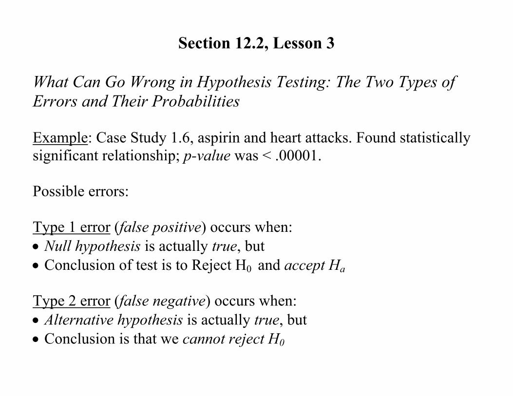
Section 12.2, Lesson 3 What Can Go Wrong in Hypothesis Testing: The Two Types of Errors and Their Probabilities Example: Case Study 1.6, aspirin and heart attacks. Found statistically significant relationship; p-value was < .00001. Possible errors: Type 1 error (false positive) occurs when: • Null hypothesis is actually true, but • Conclusion of test is to Reject H0 and accept Ha Type 2 error (false negative) occurs when: • Alternative hypothesis is actually true, but • Conclusion is that we cannot reject H0

Heart attack and aspirin example: Null hypothesis: The proportion of men who would have heart attacks if taking aspirin = the proportion of men who would have heart attacks if taking placebo. Alternative hypothesis: The heart attack proportion is lower if men were to take aspirin than if they were not to take aspirin.

Type 1 error (false positive): Occurs if there really is no relationship between taking aspirin and heart attack prevention, but we conclude that there is a relationship. Consequence: Good for aspirin companies! Possible bad side effects from aspirin, with no redeeming value.

Type 2 error (false negative): Occurs if there really is a relationship but study failed to find it. Consequence: Miss out on recommending something that could save lives! Which type of error is more serious? Probably all agree that Type 2 is more serious. Which could have occurred? Type 1 error could have occurred. Type 2 could not have occurred, because we did find a significant relationship.

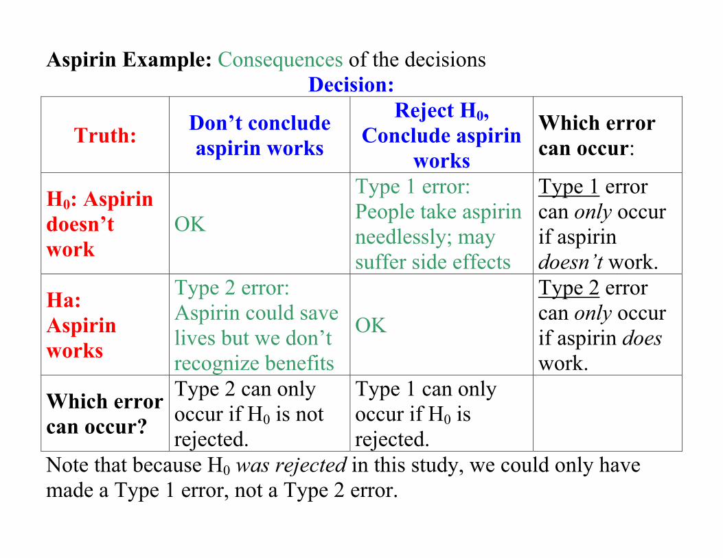
Aspirin Example: Consequences of the decisions Decision:

Truth: Don’t conclude aspirin works

Reject H0, Conclude aspirin

works

Which error can occur:

H0: Aspirin doesn’t work

OK

Type 1 error: People take aspirin needlessly; may suffer side effects

Type 1 error can only occur if aspirin doesn’t work.

Ha: Aspirin works

Type 2 error: Aspirin could save lives but we don’t recognize benefits

OK

Type 2 error can only occur if aspirin does work.

Which error can occur?

Type 2 can only occur if H0 is not rejected.

Type 1 can only occur if H0 is rejected.

Note that because H0 was rejected in this study, we could only have made a Type 1 error, not a Type 2 error.

Some analogies to hypothesis testing: Analogy 1: Courtroom: Null hypothesis: Defendant is innocent. Alternative hypothesis: Defendant is guilty Note that the two possible conclusions are “not guilty” and “guilty.” The conclusion “not guilty” is equivalent to “don’t reject H0.” We don’t say defendant is “innocent” just like we don’t accept H0 in hypothesis testing. Type 1 error is when defendant is innocent but gets convicted Type 2 error is when defendant is guilty but does not get convicted. Which one is more serious??

Analogy 2: Medical test Null hypothesis: You do not have the disease Alternative hypothesis: You have the disease Type 1 error: You don't have disease, but test says you do; a "false positive" Type 2 error: You do have disease, but test says you do not; a "false negative" Which is more serious??

Notes and Definitions: Probability related to Type 1 error:

The conditional probability of making a Type 1 error, given that H0 is true, is the level of significance α. In most cases, this is .05. However, it should be adjusted to be lower (.01 is common) if a Type 1 error is more serious than a Type 2 error.

In probability notation: P(Reject H0 | H0 is true) = α, usually .05.

Value of test statistic1.645

0.05

0

Normal, Mean=0, StDev=1

Reject null hypothesis

Do not reject null hypothesis

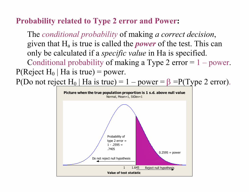
Probability related to Type 2 error and Power:

The conditional probability of making a correct decision, given that Ha is true is called the power of the test. This can only be calculated if a specific value in Ha is specified. Conditional probability of making a Type 2 error = 1 – power.

P(Reject H0 | Ha is true) = power. P(Do not reject H0 | Ha is true) = 1 – power = β =P(Type 2 error).

Value of test statistic

1.645

0.2595 = power

1

Normal, Mean=1, StDev=1Picture when the true population proportion is 1 s.d. above null value

Reject null hypothesis

Do not reject null hypothesis

.74051 - .2595 =type 2 error =Probability of

How can we increase power and decrease P(Type 2 error)? Power increases if:

• Sample size is increased (because having more evidence makes it easier to show that the alternative hypothesis is true, if it really is)

• The level of significance α is increased (because it’s easier to reject H0 when the cutoff point for the p-value is larger)

• The actual difference between the sample estimate and the null value increases (because it’s easier to detect a true difference if it’s large) We have no control over this one!

Trade-off must be taken into account when choosing α. If α is small it’s harder to reject H0. If α is large it’s easier to reject H0: • If Type 1 error is more serious, use smaller α. • If Type 2 error is more serious, use larger α.

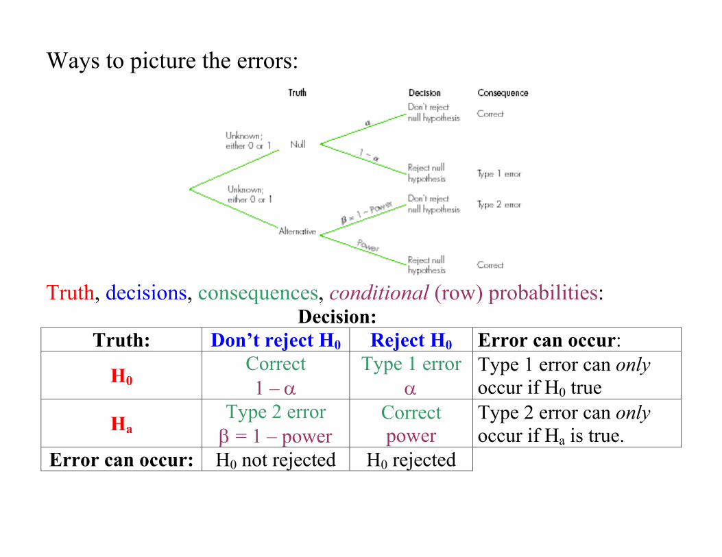
Ways to picture the errors:

Truth, decisions, consequences, conditional (row) probabilities: Decision:

Truth: Don’t reject H0 Reject H0 Error can occur:

H0 Correct 1 – α

Type 1 error α

Type 1 error can only occur if H0 true

Ha Type 2 error β = 1 – power

Correct power

Type 2 error can only occur if Ha is true.

Error can occur: H0 not rejected H0 rejected

SECTION 12.4: Test for difference in 2 proportions Reminder from when we started Chapter 9 Five situations we will cover for the rest of this quarter:

Parameter name and description Population parameter Sample statistic For Categorical Variables: One population proportion (or probability) p p̂ Difference in two population proportions p1 – p2 21 ˆˆ pp − For Quantitative Variables: One population mean µ x Population mean of paired differences (dependent samples, paired) µd d Difference in two population means (independent samples) µ1 − µ2 21 xx −

For each situation will we: √ Learn about the sampling distribution for the sample statistic √ Learn how to find a confidence interval for the true value of the parameter • Test hypotheses about the true value of the parameter

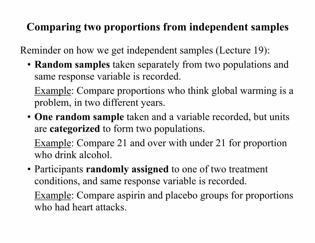
Comparing two proportions from independent samples

Reminder on how we get independent samples (Lecture 19): • Random samples taken separately from two populations and

same response variable is recorded. Example: Compare proportions who think global warming is a problem, in two different years.

• One random sample taken and a variable recorded, but units are categorized to form two populations. Example: Compare 21 and over with under 21 for proportion who drink alcohol.

• Participants randomly assigned to one of two treatment conditions, and same response variable is recorded. Example: Compare aspirin and placebo groups for proportions who had heart attacks.

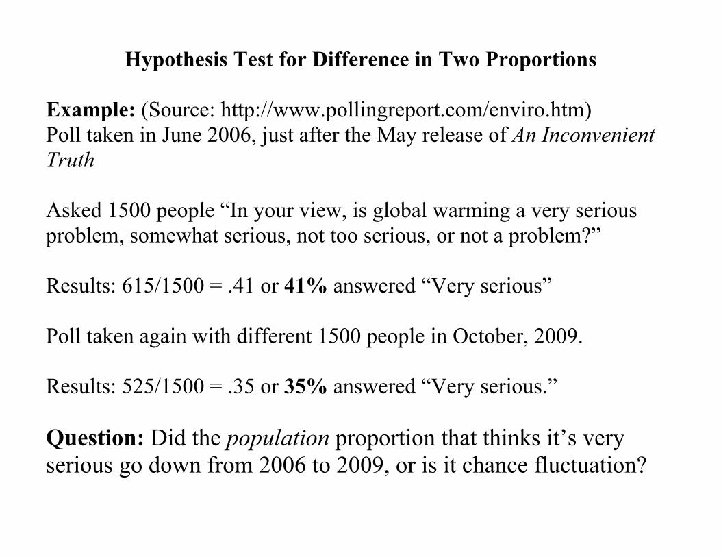
Hypothesis Test for Difference in Two Proportions

Example: (Source: http://www.pollingreport.com/enviro.htm) Poll taken in June 2006, just after the May release of An Inconvenient Truth Asked 1500 people “In your view, is global warming a very serious problem, somewhat serious, not too serious, or not a problem?” Results: 615/1500 = .41 or 41% answered “Very serious” Poll taken again with different 1500 people in October, 2009. Results: 525/1500 = .35 or 35% answered “Very serious.” Question: Did the population proportion that thinks it’s very serious go down from 2006 to 2009, or is it chance fluctuation?

Notation and numbers for the Example: Population parameter of interest is p1 – p2 where: p1 = proportion of all US adults in May 2006 who thought

global warming was a serious problem. p2 = proportion of all US adults in Oct 2009 who thought global

warming was a serious problem.

1p̂ = sample estimate from May 2006 = X1/n1 = 615/1500 = .41 2p̂ = sample estimate from Oct 2009 = X2/n2 = 525/1500 = .35

Sample statistic is 06.35.41.ˆˆ 21 =−=− pp

Five steps to hypothesis testing for difference in 2 proportions: See Summary Box on pages 531-532

STEP 1: Determine the null and alternative hypotheses.

Null hypothesis is H0: p1 – p2 = 0 (or p1 = p2); null value = 0

Alternative hypothesis is one of these, based on context: Ha: p1 – p2 ≠ 0 (or p1 ≠ p2) Ha: p1 – p2 > 0 (or p1 > p2) Ha: p1 – p2 < 0 (or p1 < p2) EXAMPLE: Did the population proportion who think global warming is “very serious” drop from 2006 to 2009? This is the alternative hypothesis. (Note that it’s a one-sided test.) H0: p1 – p2 = 0 (no actual change in population proportions) Ha: p1 – p2 > 0 (or p1 > p2; 2006 proportion > 2009 proportion)

STEP 2: Verify data conditions. If met, summarize data into test statistic.

For Difference in Two Proportions: Data conditions: pnˆ and )ˆ1( pn − are both at least 10 for both samples.

Test statistic:

error standard(null)valuenullstatisticsample −

=z Sample statistic = 21 ˆˆ pp − Null value = 0 Null standard error: • Computed assuming null hypothesis is true. • If null hypothesis is true, then p1 = p2 • We get an estimate for the common value of p using both

samples, then use that in the standard error formula. Details on next page.

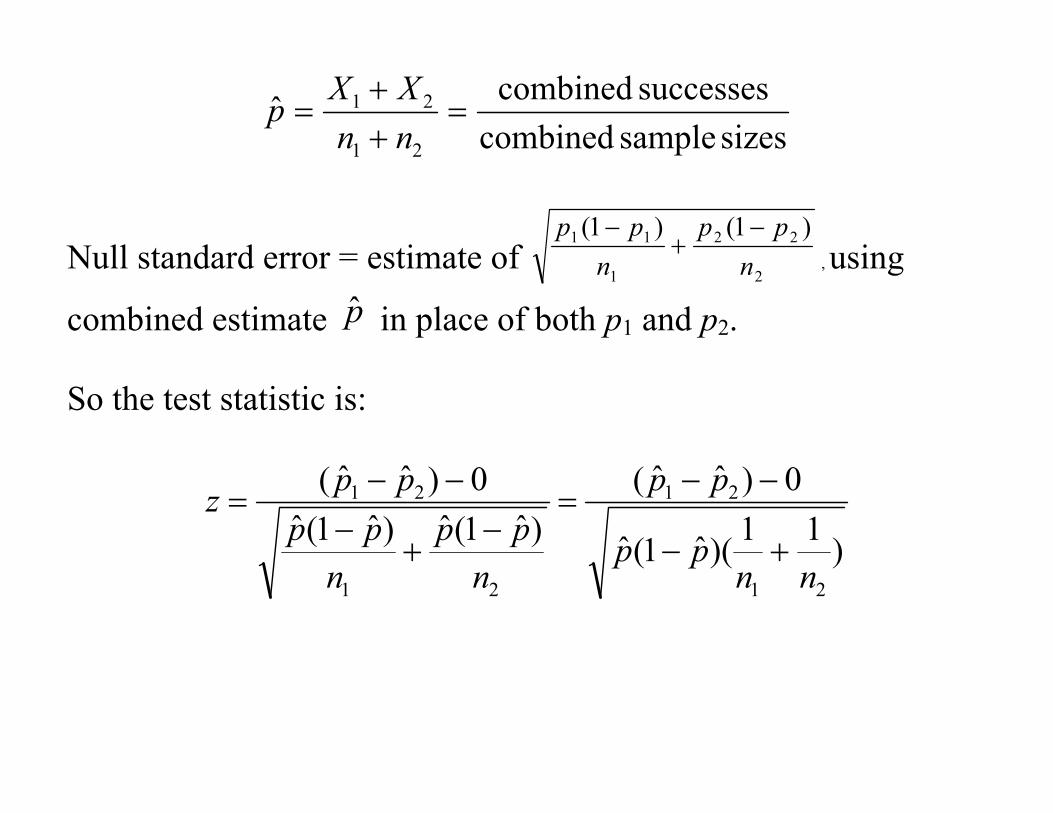
sizes sample combinedsuccesses combinedˆ

21

21 =++

=nnXXp

Null standard error = estimate of 2

22

1

11 )1()1(n

ppn

pp −+

−, using

combined estimate p̂ in place of both p1 and p2. So the test statistic is:

)11)(ˆ1(ˆ

0)ˆˆ()ˆ1(ˆ)ˆ1(ˆ

0)ˆˆ(

21

21

21

21

nnpp

pp

npp

npp

ppz+−

−−=

−+

−−−

=

Step 2 for the Example: Data conditions are met, since both sample sizes are 1500.

1 2

1 2

combined successes 615 525 1140ˆ .38combined sample sizes 1500 1500 3000

X Xpn n+ +

= = = = =+ +

Null standard error = 0177.)1500

11500

1)(38.1)(38(. =+− Test statistic:

39.30177.

006.error standard(null)

valuenullstatisticsample=

−=

−=z

Pictures: On left: Sampling distribution of 21 ˆˆ pp − when population proportions are equal and sample sizes are both 1500, showing where the observed value of .06 falls. On right: The same picture, converted to z-scores.

Possible values of p1hat - p2hat0.06

0.000350

0

Normal, Mean=0, StDev=0.0177Sampling distribution for p1hat - p2hat, when p1=p2, n1=n2=1500

Values of z3.39

0.000349

0

Normal, Mean=0, StDev=1Standard normal distribution

Note that area above 21 ˆˆ pp − = 0.06 is so small you can’t see it!

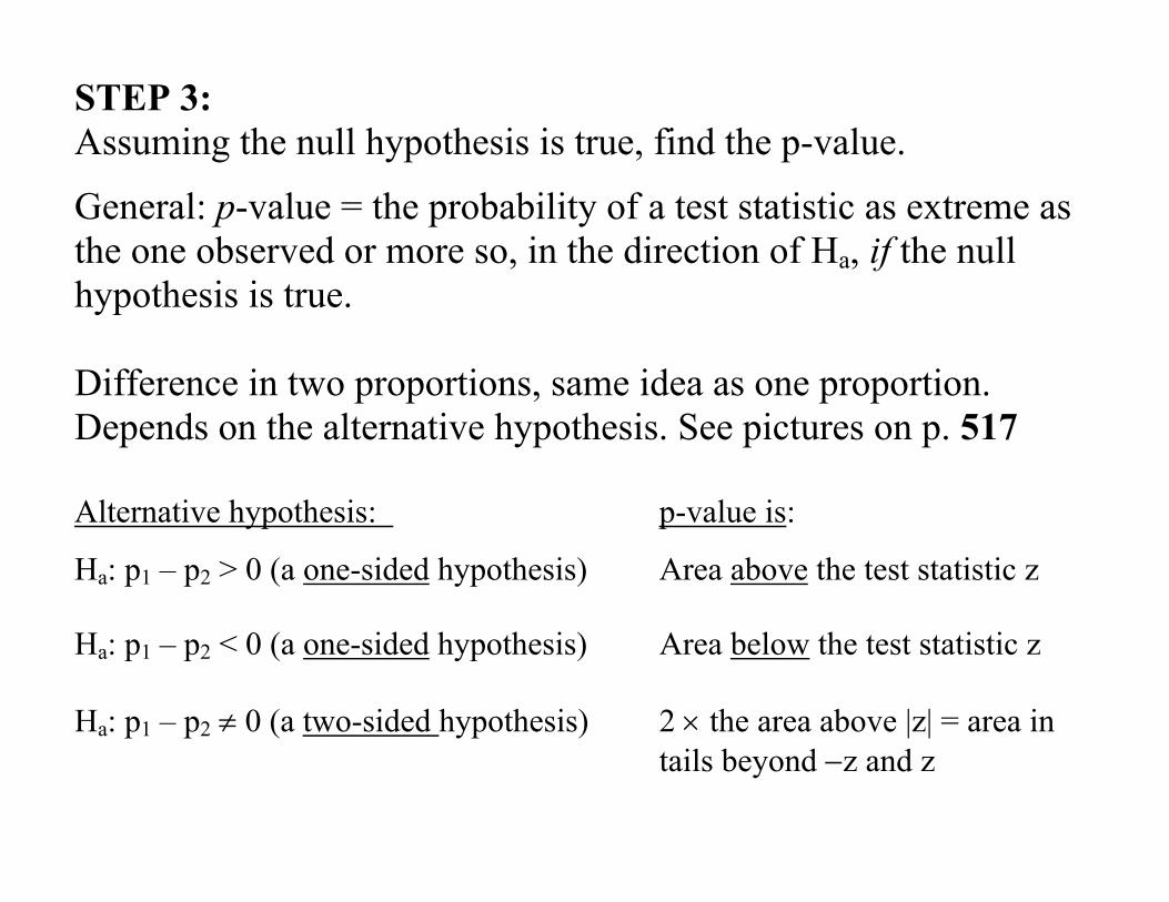
STEP 3: Assuming the null hypothesis is true, find the p-value.

General: p-value = the probability of a test statistic as extreme as the one observed or more so, in the direction of Ha, if the null hypothesis is true. Difference in two proportions, same idea as one proportion. Depends on the alternative hypothesis. See pictures on p. 517 Alternative hypothesis: p-value is:

Ha: p1 – p2 > 0 (a one-sided hypothesis) Area above the test statistic z Ha: p1 – p2 < 0 (a one-sided hypothesis) Area below the test statistic z Ha: p1 – p2 ≠ 0 (a two-sided hypothesis) 2 × the area above |z| = area in

tails beyond −z and z

Example: Alternative hypothesis is one-sided Ha: p1 – p2 > 0 p-value = Area above the test statistic z = 3.39 From Table A.1, p-value = area above 3.39 = 1 – .9997 = .0003.

STEP 4: Decide whether or not the result is statistically significant based on the p-value.

Example: Use α of .05, as usual p-value = .0003 <.05, so: • Reject the null hypothesis. • Accept the alternative hypothesis • The result is statistically significant

Step 5: Report the conclusion in the context of the situation. Example: Conclusion: From May 2006 to October 2009 there was a statistically significant decrease in the proportion of US adults who think global warming is “very serious.”

Interpretation of the p-value (for this one-sided test): It’s a conditional probability. Conditional on the null hypothesis being true (equal population proportions), what is the probability that we would observe a sample difference as large as the one observed or larger just by chance?

Specific to this example: If there really were no change in the proportion of the population who think global warming is “very serious” what is the probability of observing a sample proportion in 2009 that is .06 (6%) or more lower than the sample proportion in 2006? Answer: The probability is .0003. Therefore, we reject the idea (the hypothesis) that there was no change in the population proportion.