seasonal mortality in denmark: the role of sex and age ... · during summer, on the contrary,...

Demographic Research a free, expedited, online journal of peer-reviewed research and commentary in the population sciences published by the Max Planck Institute for Demographic Research Konrad-Zuse Str. 1, D-18057 Rostock · GERMANY www.demographic-research.org

DEMOGRAPHIC RESEARCH VOLUME 9, ARTICLE 9, PAGES 197-222 PUBLISHED 04 NOVEMBER 2003 www.demographic-research.org/Volumes/Vol9/9/ DOI: 10.4054/DemRes.2003.9.9 Descriptive Findings

Seasonal mortality in Denmark: the role of sex and age

Roland Rau

Gabriele Doblhammer

© 2003 Max-Planck-Gesellschaft.

Table of Contents

1 Introduction 198

2 Data and Methods 199

3 Results 204

4 Discussion 211

5 Conclusion 214

6 Acknowledgements 214

Notes 214

References 216

Appendix 222

Demographic Research- Volume 9, Article 9

Seasonal Mortality in Denmark:The role of sex and age

Roland Rau1

Gabriele Doblhammer2

Abstract

Our paper addresses two questions on seasonal mortality: How do women and men differwith respect to seasonal fluctuations in mortality? How does seasonality in death changewith age? The analysis is based on a sample of all Danes aged 50 and older on 1 April1968 who were followed for 30 years.

In contrast to previous studies we found remarkable differences between women andmen in their seasonal mortality patterns. Men showed larger seasonal fluctuations thanwomen indicating a higher susceptibility to environmental stressful periods.

We found that seasonality increases with age. However, we discovered again a sexdifference: women’s seasonality starts increasing at later ages than men’s.

1Max Planck Institute for Demographic Research, Konrad Zuse Str. 1, 18057 Rostock, Germany. E-mail:[email protected];

2Max Planck Institute for Demographic Research, Konrad Zuse Str. 1, 18057 Rostock, Germany. E-mail:[email protected];

http://www.demographic-research.org 197

Peter Wilhelm

Peter Wilhelm

Peter Wilhelm

Peter Wilhelm


1 Introduction

“Death strikes from every side, but not at random” (March, 1912, p. 505). While an in-dividual death may not be predicted, it is possible to make a probabilistic forecast aboutthe timing of death. In Western countries, one is most likely to die during the first fewmonths of the year. During summer, on the contrary, mortality is lowest (Aubenque et al.,1979; Feinstein, 2002; Hernández and García-Moro, 1987; Kunst et al., 1990; Lerchl,1998; Lyster, 1972; Mackenbach et al., 1992). These fluctuations “are one of the ‘deepstructures’ that identify the main environmental and cultural factors that form a givenpopulation” (Shaw, 1996, p. 100). Although climate shapes the basic seasonal pattern ofmortality, one cannot necessarily equate colder climate with larger monthly oscillations.Indeed, Canada, Russia and the Scandinavian countries show a lower percentage of ex-cess deaths during winter than, for example, the UK and many Mediterranean countries(Grut, 1987; McKee, 1989). It has been estimated for the late 1970s that about half amillion deaths per year in North America, the USSR, and Europe were cold-related (Grut,1987). It is argued that these deaths are mainly an outcome of exposure to outdoor andindoor cold; people living in rather severe climatic zones protect themselves better againstboth kinds of hazards (Donaldson et al., 1998; Donaldson and Keatinge, 2002; Donaldsonet al., 1998; Eurowinter Group, 1997, 2000; Keatinge, 1986; Keatinge et al., 1989).

Previous studies often focussed on the dampening of the seasonal fluctuations in mor-tality over time (Kunst et al., 1990; Madrigal, 1994; Marcuzzi and Tasso, 1992; Mc-Dowall, 1981). However, this trend towards de-seasonalization is not generally applicableas shown, for instance, for France and the UK until the 1970s (Aubenque et al., 1979;Sakamoto-Momiyama, 1978). As a consequence, we first examined whether seasonalityis still present in Danish mortality. Denmark may not inevitably follow the pattern of othercountries in seasonal mortality as it sets itself apart from its neighbors in mortality trends.Life expectancy, for example, rose slower than anywhere else in western Europe in the1980s (Chenet et al., 1996; Dolley, 1994). If one observes the linear increase in record lifeexpectancy during the last 160 years (1840–2000), one would expect an increase in lifeexpectancy for men by 0.222 years of age for each calendar year passed (Oeppen and Vau-pel, 2002). Chenet et al. (1996) found for the period between 1979 and 1990 (12 years)only an increase by 0.9 years in Denmark. Contrastingly, Denmark’s neighbor Swedenhad a value of 2.6 years for the same time period which is close to the expected value of2.664 years. The decelerated increase in life expectancy for Danish women drew evenmore attention: it rose by 0.35 years during that period whereas 2.916 years could havebeen expected. [Note 1] A previous study tried to explain the different developments oflife expectancy in the neighboring countries in general with “minor differences in socialand cultural factors” (Chenet et al., 1996, p. 404). The reasons for the poor performancefor female life expectancy in Denmark has been subject to much debate: most studies

198 http://www.demographic-research.org


point into the direction that it was caused by the “between wars” cohorts of women whohave the highest mortality rates for lung cancer and chronic obstructive pulmonary diseaseanywhere in Europe. These causes of death are usually associated with the high smokingprevalence of those cohorts (Jacobsen et al., 2002; Juel, 2000). [Note 2]

Instead of examining the trend over time, we analyzed in this pilot study the factors sexand age. They usually received little attention in previous studies, despite their paramountinfluences on mortality (Rogers et al., 1995, p. 7–8). A usual assumption among demog-raphers asserts that mortality measures the current conditions of the ecological and socialenvironment (Robine, 2001). According to that assessment, women and men vary in theirsusceptibility towards environmental hazards as reflected by the lower female age-specificmortality-rates throughout the life-course. Consequently, we were puzzled by the resultsof several studies on seasonality that included the factor sex. They typically found nosignificant differences between women and men in seasonality in all-cause mortality (Eu-rowinter Group, 1997; Gemmell et al., 2000; Nakai et al., 1999; Yan, 2000).

The factor age has been analyzed in more detail than sex. However, the basis ofthe data implied some problems in previous studies. Sometimes no age distinction wasmade at all (Aubenque et al., 1979; Barrett, 1990; Rosenwaike, 1966; Trudeau, 1997).In other studies the highest included age or the beginning of the last, open-ended, agecategory was chosen at an age after which most deaths in a population occur (Bull andMorton, 1978; Crombie et al., 1995; Donaldson et al., 1998; Eurowinter Group, 1997,2000; Human Life-Table Database, 2003; Huynen et al., 2001; Keatinge et al., 1989; Mc-Kee et al., 1998; Underwood, 1991). Thus, results from these studies may simplify orblur the relationship between age and seasonal fluctuations in mortality. Some studies an-alyzed heat-related mortality up into very advanced ages (Mackenbach et al., 1997; Nakaiet al., 1999), but only a few investigated overall seasonal mortality in these age-groups(Feinstein, 2002; McDowall, 1981; Näyhä, 1980). [Note 3] The general trend in thosestudies asserts an increase of seasonality with age. This fits our framework of decreasingresistance towards environmental hazards with age.

2 Data and Methods

Our data consisted of all Danes who were 50 years or older on 1 April 1968. These1,374,536 individuals were followed for 30 years until March 1998. 1,994 people werelost (censored) during the observation period (0.1 percent). 1,171,535 individuals (85.2percent) died, leaving 201,007 survivors (14.6 percent) in the end of March 1998 behind.For each individual, birth and death (or censoring) have been recorded by month and year.

We calculated winter excess mortality for the whole population following Grut (1987)(which is similar to McKee 1989) to have a descriptive and comparable measurement to



other countries in respect to the amount of possibly preventable deaths:

EWD = D−(

12× DJUL + DAUG + DSEP

3

)(1)

EWD represents the number of excess winter deaths,D is the number of all deathsduring the follow-up andDJUL, DAUG, DSEP represent the number of deaths during July,August, and September, respectively. The proportion of winter excess deaths is obtainedby computingEWD/D.

Figure 1: Cohort Distinction in a Lexis-Diagram

Our main objective was to analyze the changing risks of dying in different months ofthe year. We created a data-set that contains a person as many times as he/she has lived inmonths between April 1968 and March 1998. When using the whole Danish populationat ages 50+ this procedure would lead to a huge data-set. We therefore opted to draw arandom-sample of each cohort and sex. The final data-set included 46,293 individuals (≈3.4 percent sample). Being aware of this shortcoming of giving away information fromour data, we would like to emphasize that we understand our analysis as a first exploratorystep. Future steps will neither rely on a sample nor be restricted to the two covariates age



and sex.

Figure 2: Graphical Outline of Data-Set for Analysis by Age

We further divided the population by using four ten-year birth cohorts: the oldestcohort (Cohort I) was born between April 1878 and March 1888. In April 1968 theywere aged between 80 and 89 years and 11 months. We followed them until they reacheda maximum age of 99 years and 11 months (March 1978 to March 1988).The secondcohort(birth dates between April 1888 and March 1898) is aged 70 to 79 years and 11months in 1968 and is followed to age 99 years and 11 months (time period March 1988- March 1998).The third cohort(born April 1898 — March 1908) is aged 60 to 69 yearsand 11 months at baseline. At the end of the follow-up (March 1998) they have reachedages 90 to 99 and 11 months.The fourth cohort(born April 1908 — March 1918) is aged50 to 59 and 11 months at baseline and reaches maximum ages of 80 to 89 and 11 monthsin March 1998. Please see Figure 1 for a graphical description of this classification. Theexact numbers of individuals in each cohort by birth date, sex, and survival status aregiven in Table 1. We controlled for different length of month by standardizing all recordsto a weight of 30 days.

The age specific analysis is based on a slightly different definition of cohorts. The



goal was that every member of a specific cohort should theoretically be able to reach eachanalyzed age. For example, people inCohort III who were 60 years old in the beginningof the follow-up could attain a maximum of 90 years. Analogously, people in the samecohort aged 69 years in 1968 have no possibility to be exposed to the risk of dying at age65 anymore. Therefore, we transformed the cohorts into parallelograms as follows (seeFigure 2):

In each of the cohorts we constructed two age groups. The oldest cohort was followedfrom age 90 (time period April 1968 to April 1978) until they reached the age 94 yearsand 11 months (Fig. 2,D1). Within the same birth cohort we compared this age groupwith the 5-year age group that reached age 95 between April 1973 and April 1978 andattained a maximum age of 99 years and 11 months between March 1978 and March 1988(D2). In the second cohort the first age group consists of all those who were aged 80 inthe time period April 1968 to April 1973 and reached a maximum age of 89 years and11 months between March 1978 and March 1988 (C1). The second age group in CohortII comprises ages 90 (time period April 1978 to April 1988) to 99 years and 11 months(time period March 1988 to March 1998) (C2). The first age group in the third cohortconsists of ages 70 to 79 years and 11 months (B1), the second of ages 80 to 89 yearsand 11 months (B2). In the youngest cohort, the first age group comprises ages 60 to 69years and 11 months (A1); the second age group, ages 70 to 79 years, 11 months (A2).The time periods for the respective age groups in the two youngest cohorts are the sameas those specified in Cohort II.

We analyzed the mortality of our subjects using a logistic regression model. [Note 4]Following Allison (1995), the effects of the covariates are modeled by using Equation 2:

log(

Pit1− Pit

)= αt +

11

∑m=1

βmxi,m + δPeriodvi,t + γAgewi,t (2)

The log of the probabilityPit that the event (death) happens to individuali at timet — given that death did not happen to individuali at time t (1 − Pit) — is related toan intercept (αt) and a set of further covariates. Theβ-parameters estimate the effect of11 dummy variables representing current month with one month serving as a referencegroup. The parametersδ and γ control for period effects and for age (time-varying),respectively. The odds-ratios (the exponentiatedβ-parameters) can be used to assess ap-proximately the relative risks if the number of occurrences is rather small compared tothe risk-set (Woodward, 1999). In our analysis, we controlled for left-truncation becauseof the different ages of the subjects in the beginning of the follow-up. Whenever groupswere contrasted (women and men; different age-groups), we opted to calculate separatemodels instead of including interaction effects.



Table 1: Sample Population of follow-up from 1968 until 1998 of elderlyDanish people by cohort classification, sex, and survival status

Coh

ort

Birt

hD

ate

Sex

Aliv

ein

Per

son-

mon

ths

Sur

vivi

ngA

pril

1968

lived

Mar

ch19

98*

IA

pril

1878

—M

arch

1888

Fem

ale

2,07

214

4,25

7.0

44I

Apr

il18

78—

Mar

ch18

88M

ale

1,55

110

0,15

8.0

25

IIA

pril

1888

—M

arch

1898

Fem

ale

5,79

276

0,12

4.5

93II

Apr

il18

88—

Mar

ch18

98M

ale

4,71

550

9,10

6.5

18

IIIA

pril

1898

—M

arch

1908

Fem

ale

8,46

41,

646,

669.

595

IIIA

pril

1898

—M

arch

1908

Mal

e8,

117

1,34

1,48

1,5

80

IVA

pril

1908

—M

arch

1918

Fem

ale

6,96

61,

578,

623.

517

7IV

Apr

il19

08—

Mar

ch19

18M

ale

8,61

61,

790,

307.

015

2

I-IV

Apr

il18

78—

Mar

ch19

18F

emal

e23

,294

4,12

9,67

4.5

409

I-IV

Apr

il18

78—

Mar

ch19

18M

ale

22,9

993,

741,

053.

027

5

I-IV

Apr

il18

78—

Mar

ch19

18B

oth

46,2

9315

,741

,455

.068

4

*Coh

orts

Iand

II:S

urvi

ving

toA

ge99

Yea

rsan

d11

Mon

ths



Hewitt’s test (Hewitt et al., 1971) was employed to investigate whether the relativerisks of dying follow a seasonal pattern. This test gives ranks to each month. The value“12” is assigned to the month with the highest relative risk, and “1” to the month withthe lowest relative risk. Keeping the original order of the months (January, February, ...,December), the test statistic is the maximum rank-sum of six consecutive months. Thus,this method assumes that the year is split into two 6-months-periods with a relatively highrisk to experience the event in one half and a relatively low risk during the other half.Simulated significance levels (Hewitt et al., 1971) were applied for Hewitt’s test if exactvalues were not available (Walter, 1980).

3 Results

Monthly standardized death counts:⇒Denmark displays the typical Western pattern.

Figure 3 shows the monthly distribution of the 1,171,535 deaths of the whole data-setin percent after standardizing each month to thirty days. The bars indicate a season-ally changing pattern peaking in January (number of standardized deaths: 106,037) andreaching a minimum in August (88,395 standardized deaths). According to our definition78,375 deaths during our observation period of 30 years can be attributed to winter excessmortality or more than 2,600 deaths each year. This equals a proportion of 6.69 percentof all deaths.Monthly odds ratios for the four cohorts:⇒Seasonal fluctuations are larger in the older cohorts.

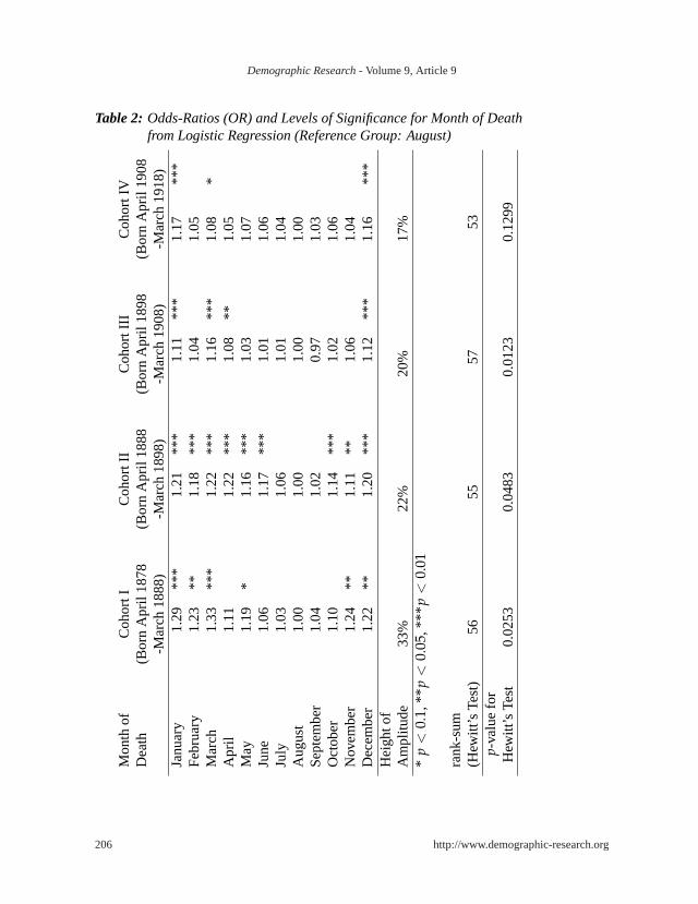
Table 2 shows the results of a logistic regression model based on our sample estimat-ing the odds-ratios (OR) for each month of the year on the risk of dying. The risk for theyoungest cohort (Cohort IV: ages 50/59 to ages 80/89) is 17% higher in January than inthe reference month August. The older the cohorts, the higher the differences between theminimum and the maximum. The height of the amplitudes increases to 34 percent in theoldest cohort (Cohort I: ages 80/89 to ages 90/99). The patterns differ in the four cohorts.The p-values for Hewitt’s test for seasonality reach an acceptable level of significanceonly for Cohorts I - III (p ≤ 0.0253). The youngest cohort (Cohort IV), on the contrary,does not seem to follow a typical seasonal pattern (p = 0.1299).



Figure 3: Distribution of Monthly Mortality in Percent after Standardizing Lengthof Month



Table 2: Odds-Ratios (OR) and Levels of Significance for Month of Deathfrom Logistic Regression (Reference Group: August)

Mon

thof

Coh

ortI

Coh

ortI

IC

ohor

tIII

Coh

ortI

VD

eath

(Bor

nA

pril

1878

(Bor

nA

pril

1888

(Bor

nA

pril

1898

(Bor

nA

pril

1908

-Mar

ch18

88)

-Mar

ch18

98)

-Mar

ch19

08)

-Mar

ch19

18)

Janu

ary

1.29

***

1.21

***

1.11

***

1.17

***

Feb

ruar

y1.

23**

1.18

***

1.04

1.05

Mar

ch1.

33**

*1.

22**

*1.

16**

*1.

08*

Apr

il1.

111.

22**

*1.

08**

1.05

May

1.19

*1.

16**

*1.

031.

07Ju

ne1.

061.

17**

*1.

011.

06Ju

ly1.

031.

061.

011.

04A

ugus

t1.

001.

001.

001.

00S

epte

mbe

r1.

041.

020.

971.

03O

ctob

er1.

101.

14**

*1.

021.

06N

ovem

ber

1.24

**1.

11**

1.06

1.04

Dec

embe

r1.

22**

1.20

***

1.12

***

1.16

***

Hei

ghto

fA

mpl

itude

33%

22%

20%

17%

*p

<0.

1,**

p<

0.05

,***

p<

0.01

rank

-sum

(Hew

itt’s

Test

)56

5557

53p-

valu

efo

rH

ewitt

’sTe

st0.

0253

0.04

830.

0123

0.12

99



Sex-specific odds ratios by season for the four cohorts:⇒ Men experience larger seasonal fluctuations in mortality than women.

Figure 4 gives the result of a similar estimation as Table 2 with two exceptions: First,we conducted separate analyzes for women and men. Second, months have been summa-rized to seasons (Winter: January, February, March;Spring: April, May, June;Summer:July, August September;Fall: October, November, December) to clarify trends.

Figure 4: Odds-Ratios and 95 % Confidence Intervals for Seasonal Mortality by Sex(Reference Group: Summer)



Figure 5: Odds-Ratios for Seasonal Mortality by Sex and Age-Group Part I(Reference Group: Summer)



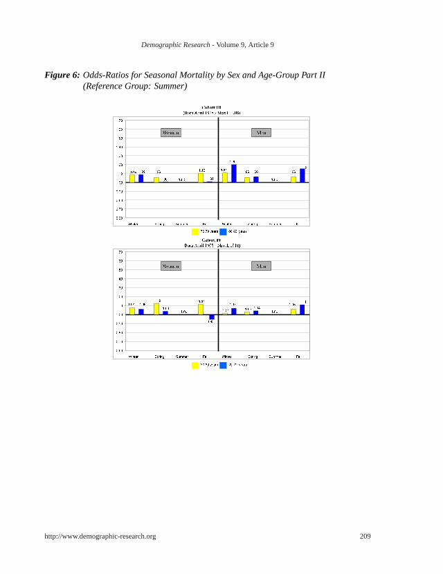
Figure 6: Odds-Ratios for Seasonal Mortality by Sex and Age-Group Part II(Reference Group: Summer)



The youngest cohort (Cohort IV: ages 50/59 to ages 80/89, time period 1968 to 1998)displays virtually no difference between the sexes. With odds-ratios of 1.08 for womenand 1.07 for men, the mortality risk is highest for both sexes in winter. Cohort III (ages60/69 to ages 90/99, time period 1968 to 1998), which is on average 10 years older thanCohort IV, shows a similar pattern with a peak in winter and a trough in summer for bothsexes. However, the relative mortality risk is remarkably higher for men than for women(OR winter: 1.14 vs 1.08; OR spring: 1.07 vs. 1.03; OR fall: 1.10 vs 1.06). Since bothcohorts cover the same time period the increase in the seasonality must be due to differ-ences in age.

In Cohort II (ages 70/79 to age 99, time period 1968 to 1988/1989), men face excessmortality of 20 percent in winter and 21 percent in spring, women’s excess mortality is1.14 and 1.11, respectively. The oldest people (Cohort I: ages 80/89 to age 99, time period1968 to 1978/1988) are reversing the trend. Men’s seasonal fluctuations are smaller thanwomen’s and their trough changed from summer to spring (OR spring: 0.97). Women inthat cohort faced higher relative risks during each season than in any other cohort, reach-ing a maximum in winter with a relative risk of 31 percent in winter compared to summer.

Since the oldest cohort only covers the time period 1968/1973 to 1978/ 1983 (opposedto the other cohorts covering 1968/1978 to 1988/98), we cannot distinguish whether theparticular pattern in this cohort is due to age effects or period effects.

Sex and age-specific odds ratios by season for the four cohorts:⇒Seasonal fluctuations in mortality start increasing at later ages for women thanfor men.

Figures 5 and 6 show the effect of age on the seasonality in mortality. Men, generallyspeaking, exhibit an increase of seasonal mortality fluctuations with age. In the youngestcohort the relative mortality risk for septagenarians compared to 60-69 year olds increasedby 1 percentage point in spring, 5 percentage points in fall, and by 6 percentage points inwinter. The increase in fluctuations further intensifies in the oldest cohort. In addition,we observe an intermediary peak in mortality during summer among the oldest men.

Women show a more complicated pattern than men. In Cohort IV, they have a de-creasing trend in seasonality from 60-69 years to 70-79 years. Also the comparison of70-79 year olds with 80-89 year olds in Cohort III yields the same result: either therewas almost no change at all (winter) or the estimates became smaller (spring and fall).Cohorts I and II, however, show an obvious increase of seasonality in mortality with age.The increase from octagenarians to nonagenarians amounts to 5 percentage point in win-ter (1.13 to 1.18), 9 percentage points in spring (1.12 to 1.21), and 5 percentage points infall (1.10 to 1.15). By comparing 90-94 year old with 95-99 year old women in Cohort I,the odds-ratios increase with age from 1.31 to 1.58 in winter, 1.09 to 1.64 in spring, and



1.01 to 1.57 in fall. Contrary to men, we do not observe a summer peak among women.

4 Discussion

Before discussing the results, it is useful to briefly point out the advantages of the study.Some of the potential shortcomings will be discussed at the end of this section. The designof our data-set makes our analysis unique. The major drawback of previous longitudinalstudies was the non-availability of the exact risk-set. Either researchers used deaths counts(e.g. Gemmell et al., 2000; Trudeau, 1997) or interpolated data to obtain the specificpopulation at risk (e.g. Mackenbach et al., 1992; Marshall et al., 1988). To our knowledge,only one previous longitudinal study used exact exposures and occurrences of events (vanRossum et al., 2001). However, our analysis has the advantage that it is based on a sampleof the whole population and is, therefore, not restricted to one occupation (civil servants)and one sex (men) (van Rossum et al., 2001).

We found that mortality in Denmark follows the well-known seasonal pattern of coun-tries in the Northern Hemisphere. Denmark is experiencing 2,612 winter excess deathsannually, which corresponds to a proportion of 6.69 percent of all deaths. Denmark ison level terms with the US in 1978 (Grut, 1987) and fares better compared to some otherEuropean countries like Ireland (14.6%) and Portugal (13.7%) during the period 1976–83. However, a comparison (McKee, 1989) with its neighboring countries in the Balticlike West Germany (5.4%), Sweden (5.4%), Norway (3.9%), and Finland (3.8%) during1976–84 lets us conclude that further progress can be made in Denmark in reducing theannual cold-related death toll.

It is open to discussion how large the effect of saving lives in winter on mortality ingeneral actually is. Two extreme opinions are imaginable. The true effect will lie some-where in between: either one assumes that the subject is in a frail condition and wouldhave died anyway relatively soon. The other assumption would be that the individual doesnot differ in his/her robustness from the rest of the population. Saving a life in the lattercase would be “perfect repair” in terms of reliability engineering. Further analysis on theactual causes of death could shed some light on this question. If accidents and infectiousdiseases dominated the seasonal fluctuations, the overall effect could rather tend towardsthe “perfect repair extreme”. Contrastingly, if chronic diseases mainly shaped the sea-sonal pattern, the effect on reducing overall mortality would either be relatively small orit would require more efforts in medicine, public health and general living improvementsto obtain the same effect as in the other case where relatively inexpensive interventionslike vaccinations may result in remarkable improvements.

We find that age plays an important role for seasonal mortality. As our cohorts wereconstructed with a 10-year-age-difference between successive cohorts, we could identify



an increase with age in the amplitude of the monthly mortality risks. But not only theheights of the fluctuations were increasing. Also the seasonal pattern changed. We canmake a broad distinction between the relatively older cohorts (Cohorts I and II) on the onehand and the younger cohorts (Cohorts III and IV) on the other hand. In the older cohorts,the trough is restricted to the three warmest months (July-September). Throughout theremainder of the year, excess mortality is relatively high. The younger group, conversely,shows a different pattern. The trough ranges approximately from spring until early fall.Peaks in mortality can only be found in the coldest months. This result may indicate achange in the sensitivity towards environmental hazards with age: in the two younger co-horts, only the extreme cold weather proved to be dangerous for the Danish. If we look,though, at the two older cohorts, we can see that anything else but summer climate seemsto be perilous for survival for women.

The intermediary summer peak for men suggests that the oldest men are affected byextreme climatic conditions in general: cold weather in winter as well as hot spells duringsummer. We suspect that this changing pattern has been missed by previous studies eitherbecause of the limited age-range they investigated or by an underrepresentation of peopleat very advanced ages.

The slight mortality dip in all cohorts in February suggests a similar explanation ashypothesized for historical English populations by Oeppen (Oeppen, 2003): while peopledying in January rather die of immediate causes of the cold climate, deaths in March aredue to the accumulation of detrimental effects during the cold season.

Our data helps to explain the surprising result of previous studies which found no sexdifferences in relation to seasonal mortality (Eurowinter Group, 1997; Gemmell et al.,2000; Nakai et al., 1999; Yan, 2000): we find the same result — but only for the youngestcohort (Cohort IV). In the remaining three cohorts women and men differ to a large extent.We can therefore claim that the limited age-range used in previous studies is too narrowto conclude that the susceptibility towards cold-related hazards does not differ betweenwomen and men.

In Cohorts III and II, which are on average about 10 and 20 years older than Cohort IV,seasonal fluctuations are considerably larger for men than for women. This suggests thatmen at advanced ages are more susceptible to environmental hazards than women. At firstsight, the oldest cohort (Cohort I) seems to contradict this finding: women’s fluctuationsoutstrip men’s oscillations. To interpret this, we should keep in mind that changes in pop-ulation parameters can be caused by three different forces (Vaupel and Canudas Romo,2002). The first explanation refers to the small sample size of our data for the logisticregression model. A direct effect (second potential explanation) assumes that men havebecome weak to such an extent that any unfavorable conditions may act as lethal. We findsupport for this explanation in the intermediary summer peak indicating heat-related mor-tality. This follows a previous finding for Texas (Greenberg et al., 1983). Among all men,



the oldest displayed the highest death rates during heat spells. However, Mackenbach andhis colleagues (Mackenbach et al., 1997) found contradictory evidence: women’s excessmortality during hot periods is higher than men’s. Additionally, age “does not appearto be consistently related to excess mortality at high outside temperatures” (Mackenbachet al., 1997, p. 1298). Due to these opposing views in the literature, we suppose that ourfinding may be the outcome of a compositional effect, too (third possible explanation): asthe frail tend to die earlier, the male survivors in the oldest cohort (Cohort I) are a selectedsubsample of their initial birth cohort being more robust on average.

Among men, seasonal mortality fluctuations increase with age. We suggest two expla-nations for the stationary or even decreasing trend for women in the two younger cohorts:either women actually have increasing seasonal fluctuations in mortality but this trend isoffset by beneficial period-effects. However, this explanation seems to be less likely asit implies that some secular events had positive consequences for women in those age-ranges but neither at later ages nor for men. We rather support the opposing idea thatthe aging process in the younger observed age-groups does not affect the relatively strongresistance of women towards changing environmental hazards. At later ages women alsoface an increasing susceptibility with age. Our interpretation therefore is that womenas well as men show larger seasonal fluctuations in mortality as they age. The maindifferences are that women’s susceptibility starts at later ages and is restricted to coldtemperatures. Men, on the contrary, show increases with age already at younger ages. Inthe oldest observed age-categories, men have become not only susceptible to cold outsidetemperatures but to any unfavourable climatic conditions (e.g. summer heat).

The data of our analysis can be criticized in some respects. First, we rarely foundsignificant values for the analysis by age. Our remaining tables and figures, however, giveus several indications that the general trend we observed is correct and the lack of signifi-cant values can be primarily attributed to our sample size. Secondly, causes of death werenot available. Their inclusion would have helped us, for example, to verify whether thedip in mortality in February is actually due to the different mechanisms mentioned above.Further analyses on seasonal mortality should aim to incorporate the whole population,causes of death and risk factors such as housing and deprivation already mentioned in theliterature (Aylin et al., 2001; Clinch and Healy, 2000; Eurowinter Group, 1997; Keatingeand Donaldson, 2001; Lawlor et al., 2002, 2000a,b; Olsen, 2001; Shah and Peacock, 1999;Wilkinson et al., 2001). Using those covariates in a population-based longitudinal studywith exact risk-set will improve our understanding of the mechanisms regulating seasonalmortality that are still discussed ambiguously.



5 Conclusion

This study analyzed seasonal mortality in Denmark which is relatively high compared toits neighboring countries. We have shown that the previous assessment that women andmen do not differ with respect to seasonal fluctuations in mortality tends to be an oversim-plification. Men seem to be more susceptible to hazardous environmental conditions thanwomen. This is what one could expect from the generally lower female mortality ratesthroughout the life-course. We found evidence that seasonality increases with age. How-ever, the pattern varies between women and men. Women’s seasonal fluctuations startincreasing at later ages than men’s. Compared to women, men seem to be susceptible notonly to cold weather but also to extreme hot climatic conditions.

Tackling seasonal mortality will gain further relevance for public health researchersfrom two directions. First, the chances to survive into ages where seasonal fluctuationsin mortality reach remarkable levels are increasing (Kannisto et al., 1994; Vaupel, 1997).Secondly, the vast amount of literature on risk factors and the smaller fluctuations inregions with colder climate let us conclude that the annual amount of excess mortalitymay be reducible by preventive health and safety measures (Trudeau, 1997).

6 Acknowledgements

The authors would like to thank Francesco C. Billari for his valuable technical commentsand two anonymous referees; the readability of the paper benefitted from the advice ofMaggie Kulik and Uta Ziegler.

Notes

1. Oeppen and Vaupel (2002) calculated for women an increase of 0.243 years of age forevery calendar year passed.

2. It has been seriously suggested but also heavily contested that the reason for the highsmoking prevalence of the “between wars” generation of Danish women is caused by thebad role model effect of the smoking Queen Margrethe II (Jacobsen et al., 2001; Kesteloot,2001; Madsen, 2001).

3. An exception is represented by the article of Robine and Vaupel (2001) which analyzesexclusively people above ages 100 and 110, respectively.



4. Although death can happen at any point in time, our data-set specifies only month ofdeath. Thus, from a theoretical point of view, a continuous-time approach can not bejustified (Allison, 1982) because we are interested in analyzing the effect of a time-varyingcovariate (current month) which changes its values at exactly the same intervals of time asthe transition variabledeath. In practice, the differences between our logistic regressionmodel and a Cox proportional hazards model turned out to be rather negligible. See Table1 in the Appendix.



References

Allison, P. D. (1982). Discrete-time methods for the analysis of event histories.Sociolog-ical Methodology 13, 61–98.

Allison, P. D. (1995).Survival Analysis Using the SAS System. Cary, NC: SAS InstituteInc.

Aubenque, M., P. Damiani, and H. Massé (1979). Variations saisonnières et sérieschronologiques des causes de décès en France de 1900 à 1972.Cahiers de Sociolo-gie et de Démographie Médicales 19, 17–22.

Aylin, P., S. Morris, J. Wakefield, A. Grossinho, L. Jarup, and P. Elliott (2001). Temper-ature, housing, deprivation and their relationship to excess winter mortality in GreatBritain, 1986–1996.International Journal of Epidemiology 30, 1100–1108.

Barrett, R. E. (1990). Seasonality in vital processes in a traditional Chinese population.Modern China 16, 190–225.

Bull, G. and J. Morton (1978). Environment, temperature and death rates.Age andAgeing 7, 210–224.

Chenet, L., M. Osler, M. McKee, and A. Krasnik (1996). Changing life expectancy inthe 1980s: why was Denmark different from Sweden?Journal of Epidemiology andCommunity Health 50, 404–407.

Clinch, J. P. and J. D. Healy (2000). Housing standards and excess winter mortality.Journal of Epidemiology and Community Health 54, 719–720.

Crombie, D., D. Fleming, K. Cross, and R. Lancashire (1995). Concurrence of monthlyvariation of mortality related to underlying cause in europe.Journal of Epidemiologyand Community Health 49, 373–378.

Dolley, M. (1994). Denmark tries to raise life expectancy.British Medical Journal 308,737–738.

Donaldson, G., S. Ermakov, Y. Komarov, and W. Keatinge (1998). Cold related mortali-ties and protection against cold in Yakutsk, eastern Siberia: observation and interviewstudy.British Medical Journal 317, 978–982.

Donaldson, G. and W. Keatinge (2002). Excess winter mortality: influenza or cold stress?observational study.British Medical Journal 324, 89–90.



Donaldson, G., V. Tchernjavskii, S. Ermakov, K. Bucher, and W. Keatinge (1998). Wintermortality and cold stress in Yekaterinburg, Russia: interview study.British MedicalJournal 316, 514–518.

Eurowinter Group (1997). Cold exposure and winter mortality from ischaemic heartdisease, cerebrovascular disease, respiratory disease, and all causes in warm and coldregions of Europe.Lancet 349, 1341–1346.

Eurowinter Group (2000). Winter mortality in relation to climate.International Journalof Circumpolar Health 59, 154–159.

Feinstein, C. A. (2002). Seasonality of deaths in the U.S. by age and cause.DemographicResearch 6, 469–486.

Gemmell, I., P. McLoone, F. Boddy, G. J. Dickinson, and G. Watt (2000). Seasonalvariation in mortality in Scotland.International Journal of Epidemiology 29, 274–279.

Greenberg, J. H., J. Bromberg, C. Reed, T. L. Gustafson, and R. A. Beauchamp (1983).The epidemiology of heat-related deaths, Texas—1950, 1970–79, and 1980.AmericanJournal of Public Health 73, 805–807.

Grut, M. (1987). Cold-related death in some developed countries.The Lancet(8526),212. 24 January 1987.

Hernández, M. and C. García-Moro (1986–1987). Seasonal distribution of mortality inBarcelona (1983-1985).Antropol. Port. 4–5, 211–223.

Hewitt, D., J. Milner, A. Csima, and A. Pakula (1971). On Edwards’ criterion of seasonal-ity and a non-parametric alternative.British Journal of Preventive Social Medicine 25,174–176.

Human Life-Table Database (2003, April). Data by country: Denmark. Con-tributions from Väinö Kannisto and Danmarks Statistik, accessible online at:http://www.lifetable.de.

Huynen, M. M., P. Martens, D. Schram, M. P. Weijenberg, and A. E. Kunst (2001). Theimpact of heat waves and cold spells on mortality rates in the Dutch population.Envi-ronmental Health Perspectives 109, 463–470.

Jacobsen, R., A. Jensen, N. Keiding, and E. Lynge (2001). Queen Margrethe ii andmortality in Danish women.The Lancet 358, 75.



Jacobsen, R., N. Keiding, and E. Lynge (2002). Long term mortality trends behind lowlife expectancy of Danish women.Journal of Epidemiology and Community Health 56,205–208.

Juel, K. (2000). Increased mortality among Danish women: population based registerstudy.British Medical Journal 321, 349–350.

Kannisto, V., J. Lauritsen, A. R. Thatcher, and J. W. Vaupel (1994). Reductions in mortal-ity at advanced ages: Several decades of evidence from 27 countries.Population andDevelopment Review 20, 793–810.

Keatinge, W. (1986). Seasonal mortality among elderly people with unrestricted homeheating.British Medical Journal 293, 732–733.

Keatinge, W., S. Coleshaw, and J. Holmes (1989). Changes in seasonal mortality withimprovements in home heating in England and Wales from 1964 to 1984.InternationalJournal of Biometeorology 33, 71–76.

Keatinge, W. and G. Donaldson (2001). Warm housing is not enough (letters).BritishMedical Journal 323, 166.

Kesteloot, H. (2001). Queen Margrethe ii and mortality in Danish women.TheLanceet 357, 871–872.

Kunst, A., C. Looman, and J. Mackenbach (1990). The decline in winter excess mortalityin the Netherlands.International Journal of Epidemiology 20, 971–977.

Lawlor, D., R. Maxwell, and B. Wheeler (2002). Rurality, deprivation, and excess wintermortality: an ecological study.Journal of Epidemiology and Community Health 56,373–374.

Lawlor, D. A., D. Harvey, and H. G. Dews (2000a). Investigation of the associationbetween excess winter mortality and socio-economic deprivation.Journal of PublicHealth Medicine 22, 176–181.

Lawlor, D. A., D. Harvey, and H. G. Dews (2000b). Investigation of the associationbetween excess winter mortality and socio-economic deprivation.Journal of PublicHealth Medicine 22, 176–181.

Lerchl, A. (1998). Changes in the seasonality of mortality in germany from 1946 to 1995:the role of temperature.International Journal of Biometeorology 42, 84–88.

Lyster, W. (1972). The altered seasons of death in America.Journal of Biosocial Sci-ence 4, 145–151.



Mackenbach, J., A. Kunst, and C. Looman (1992). Seasonal variation in mortality in TheNetherlands.Journal of Epidemiology and Community Health 46, 261–265.

Mackenbach, J. P., V. Borst, and J. M. Schols (1997). Heat-related mortality amongnursing-home patients.The Lancet 349, 1297–1298.

Madrigal, L. (1994). Mortality seasonality in Escazú, Costa Rica, 1851–1921.HumanBiology 66, 433–452.

Madsen, S. (2001). Queen Margrethe ii and mortality in Danish women.The Lancet 358,75.

March, L. (1912). Some researches concerning the factors of mortality.Journal of theRoyal Statistical Society 75, 505–538.

Marcuzzi, G. and M. Tasso (1992). Seasonality of death in the period 1889-1988 in theVal di Scalve (Bergamo Pre-Alps, Lombardia, Italy).Human Biology 64, 215–222.

Marshall, R. J., R. Scragg, and P. Bourke (1988). An analysis of the seasonal variation ofcoronary heart disease and respiratory disease mortality in New Zealand.InternationalJournal of Epidemiology 17, 325–331.

McDowall, M. (1981). Long term trends in seasonal mortality.Population Trends 26,16–19.

McKee, C. M. (1989). Deaths in winter: Can Britain learn from Europe?EuropeanJournal of Epidemiology 5(2), 178–82.

McKee, M., C. Sanderson, L. Chenet, S. Vassin, and V. Shkolnikov (1998). Seasonalvariation in mortality in Moscow.Journal of Public Health Medicine 20, 268–274.

Nakai, S., T. Itoh, and T. Morimoto (1999). Deaths from heat-stroke in Japan: 1968–1994.International Journal of Biometeorology 43, 124–127.

Näyhä, S. (1980).Short and medium term variations in mortality in Finland. Ph. D.thesis, Department of Public Health Service, University of Oulu, Finland.

Oeppen, J. (2003). personal communications. Cambridge Group for the History of Pop-ulation and Social Structure, Cambridge, UK.

Oeppen, J. and J. W. Vaupel (2002). Broken Limits to Life Expectancy.Science 296,1029–1031>.



Olsen, N. D. (2001). Prescribing warmer, healthier homes (Editorial).British MedicalJournal 322, 748–749.

Robine, J.-M. (2001). A new biodemographic model to explain the trajectory of mortality.Experimental Gerontology 36, 899–914.

Robine, J.-M. and J. Vaupel (2001). Supercentenarians: slower ageing individuals orsenile elderly?Experimental Gerontology 36, 915–930.

Rogers, R. G., R. A. Hummer, and C. B. Nam (1995).Living and Dying in the USA. Be-havioral, Health and Social Differentials of Adult Mortality. San Diege, CA: AcademicPress.

Rosenwaike, I. (1966). Seasonal variation of deaths in the United States, 1951–1960.Journal of the American Statistical Association 61, 706–719.

Sakamoto-Momiyama, M. (1978). Changes in the seasonality of human mortality: Amedico-geographical study.Social Science and Medicine 12, 29–42.

Shah, S. and J. Peacock (1999). Deprivation and excess winter mortality.Journal ofEpidemiology and Community Health 53, 499–502.

Shaw, B. D. (1996). Seasons of Death: Aspects of Mortality in Imperial Rome.Journalof Roman Studies 86, 100–138.

Trudeau, R. (1997). Monthly and daily patterns of death.Health Reports (StatisticsCanada) 9, 43–50.

Underwood, J. H. (1991). Seasonality of vital events in a Pacific island population.SocialBiology 38, 113–126.

van Rossum, C. T., M. J. Shipley, H. Hemingway, G. D. E., J. P. Mackenbach, and M. J.Marmot (2001). Seasonal variation in cause-specific mortality: Are there high-riskgroups? 25-year follow-up of civil servants from the first Whitehall study.InternationalJournal of Epidemiology 30, 1109–1116.

Vaupel, J. W. (1997). The remarkable improvements in survival at older ages.Philosophi-cal Transactions of the Royal Society of London: Biological Sciences 352, 1799–1804.

Vaupel, J. W. and V. Canudas Romo (2002). Decomposing demographic change intodirect vs. compositional components.Demographic Research 7, 1–14.

Walter, S. (1980). Exact significance levels for Hewitt’s test for seasonality.Journal ofEpidemiology and Community Health 34, 147–149.



Wilkinson, P., M. Landon, B. Armstrong, S. Stevenson, S. Pattenden, M. McKee, andT. Fletcher (2001).Cold comfort. The social and environmental determinants of excesswinter death in England, 1986–96. Bristol, UK: Policy Press.

Woodward, M. (1999).Epidemiology. Study Design and Data Analysis. Boca Raton, FL:Chapman and Hall / CRC.

Yan, Y. Y. (2000). The influence of weather on human mortality in Hong Kong.SocialScience and Medicine 50, 419–427.



A Appendix

Table 1: Cox-Proportional-Hazards Model and Binary Logistic Regression yieldthe same results in practice. An example from estimating the effectof current month on the chance of dying for Cohort I.

ModelMonth Cox-Proportional-Hazards Binary Logistic Regressionof Death (Continuous Time) (Discrete Time)January 0.2516 0.2517February 0.2060 0.2070March 0.2824 0.2867April 0.1016 0.1005May 0.1725 0.1725June 0.0621 0.0607July 0.0335 0.0332August Reference Group Reference GroupSeptember 0.0421 0.0429October 0.0977 0.0966November 0.2144 0.2156December 0.1954 0.1949


seasonal mortality in denmark: the role of sex and age ... · during summer, on the contrary,...

Documents