seasonal migration and the effectiveness of micro-credit...

Seasonal Migration and the Effectiveness ofMicro-credit in the Lean Period : Evidence from

Bangladesh ∗

ABU SHONCHOY†.The University of New South Wales

April 30, 2010

Abstract

This paper investigates the relationship between access to micro-credit and tem-porary seasonal migration, an issue which is largely ignored in the standard rural-urban migration literature. Seasonal migration due to natural disasters or agri-cultural downturns is a common phenomenon in developing countries. Usingprimary data from a cross-sectional household survey from the northern part ofBangladesh, this study quantifies the factors that influence such migration deci-sions. Seasonal migration is a natural choice for individual suffering periodic hard-ship. However, due to strong loan repayment rules, those who have prior access tomicro-credit have no such option. I find that there is no significant difference in in-come in lean period between those who have access to micro-credit and those whodo not. Households that take the decision to migrate while having access to micro-credit earn significantly more than households who only have micro-credit in thelean period. In addition, this paper finds that network effects play a significantrole influencing the migration decision, with the presence of kinsmen at the placeof destination having considerable impact. The results have numerous potentialpolicy implications, including the design of typical micro-credit schemes.Keywords : Lean period; Seasonal migration; Micro-credit; Bangladesh; Programevaluation; Matching methods.JEL Classification : J62, J64, J65, O15, O18, R23.

∗Acknowledgement : I am extremely thankful to Mr. Abu Z. Shahriar and Ms. Sakiba Zeba for per-mitting me to use the data, and to BRAC University for funding the research. Thanks to Kevin J. Fox,Ian Walker, Denzil Fiebig, Raja Junankar, Arghya Ghosh, Elisabetta Magnani and Suraj Prasad for show-ing interest and giving me numerous ideas to fulfill this research. My heartfelt thanks goes to them. Ialso benefited from insightful discussions with the participants of the conference on Bangladesh in the 21stcentury at Harvard University, Cambridge, USA, the 4th IZA/World Bank Conference on Employment and De-velopment in Bonn, Germany, and the 5th Australasian Development Economics Workshop at the University ofMelbourne, Australia. Usual disclaimers apply.†Email:[email protected]

1

http://research.economics.unsw.edu.au/ashonchoy/

1 Introduction

This paper examines the relationship between access to micro-credit and temporaryseasonal migration. This is an issue which has great policy relevance, yet is largely over-looked in the literature. Hence, the aim of this paper is to better understand the causesof seasonal migration, to establish the relationship of migration with micro-credit, toevaluate the characteristics of seasonal migrants and to quantify the effects of the fac-tors influencing seasonal migration decisions. In particular, I test the effectiveness ofmicro-credit programs in the lean period and the role played by networks (kinship) inthe seasonal migration decision.

In the standard rural-urban migration literature, scholars primarily focus on perma-nent internal migration and its economic, social and demographic significance. Veryfew studies have discussed temporary internal migration, which is variously knownas ‘seasonal migration’, ‘circular migration’, or ‘oscillatory migration’. Evidence ofthis phenomenon exists in many regions and particularly in the developing countriesof Africa (Elkan 1959, 1967; Guilmoto 1998), Asia (Hugo 1982; Stretton 1983; Desh-ingkar and Start 2003; Rogaly et al. 2002; Rogaly and Coppard 2003) and South America(Deutsch et al. 2003). People move from rural areas to nearby cities or towns for a shortperiod of time during lean periods in an attempt to survive and maintain their familyin such difficult times. Lean periods can occur as a result of agriculture cycles or natu-ral disasters, such as droughts, floods, cyclones, climate change and river erosion, andtemporary migration is an important livelihood strategy for a large number of poorrural people in developing countries.

In the case of seasonal downturns or shocks, a person may prefer a temporary moveto a permanent one because such a decision offers an opportunity to combine villagebased existence with urban opportunities. Faced with highly seasonal labor demand,villagers may see temporary migration to urban areas as a relatively practical and ratio-nal strategy to cope with seasonal downturns and natural shocks. The most importantfactor, resulting in a temporary move rather than a permanent one, however is the re-versal of the urban-rural wage differential that occurs during the peak labor demandseason in the agricultural sector.

Evidence from different countries suggests that the temporary mobilization of laborfrom rural to urban areas has important socio-economic implications. Migration re-duces the inequality in the rural area due to the flow of remittances from the migrationdestinations. This flow, which is quite regular, is unlikely to occur with permanent ruralto urban migration, and such a flow has a large impact on rural families who throughthis money can afford the necessities of life. Return migrants may also diffuse ideas,information and knowledge which might play a vital role in the rural developmentprocess.

Temporary migrants, however, cause congestion and other social problems in ur-ban areas and policy makers have insufficient information about the number of peoplemigrating temporarily to tackle these problems. Seasonal migrants are very difficult todetect and the definition is not a clear one; hence, they are typically excluded from na-

2

tional surveys. As a result, it is difficult to implement effective policies to accommodateseasonal migrants.

A recent policy innovation in developing countries has been the emergence of micro-credit in poverty alleviation. It is argued that if given access to credit, small entrepreneursfrom poor households will find opportunities to engage in viable income-generating ac-tivities and alleviate their own poverty. Various studies on the impact of micro-credit indeveloping countries have found evidence of consumption smoothing, asset building(Pitt and Khandker 1998) and the reduction of poverty (Khandker 2005). Conversely,using the same data set as Pitt and Khandker (1998), Morduch (1999) found that the av-erage impact of micro-credit is ‘non-existent’. Similarly Navajas et al. (2000) concludedthat micro-credit is largely unsuccessful in reaching the poor and the vulnerable. In sit-uations like lean period shocks, where migration is a natural response, the strict weeklyloan repayment rules of Micro-credit Institutions (MFIs) can hamper this process, re-ducing the ability of borrowers to react to a shock. A natural extension of this studyis thus to explore the effectiveness of micro-credit for the poor during the lean period,since micro-credit authorities do not address such problems when making loans. Theimpact of micro-credit and migration on income during the lean season hardship wasestimated by using a set of ‘quasi experiments’ and semi-parametric matching tech-niques.

Primary data collected from the northern part of Bangladesh is used in this paper. Arandom cross-section household survey was conducted in January 2006 by Abu Shon-choy, Abu Z. Shahriar, Sakiba Zeba and Shaila Parveen as part of a project undertakenby the Economics and Social Sciences Research Group (ESSRG) of BRAC University.The study team chose the Kurigram district of northern Bangladesh because of somedistinctive features. Kurigram is mainly an agri-based, severely poverty-stricken areaof Bangladesh that is prone to natural disasters.1 Due to the agricultural cycle, farmershave very little work to do on the farms after the plantation of the Aman in September-October.2 As a result, a large number of agricultural workers become jobless everyyear and decide to migrate temporarily. Such migrants tend to get work in the urbaninformal sector and work mainly as day laborers or street vendors. AlThough the ur-ban standard of living is typically a bare minimum for these migrants, they prefer thisoption to staying in the village with no income at all.

Pioneering work on seasonal migration in Bangladesh has been conducted by Shahriaret al. (2006). Unfortunately, the study did not produce efficient and consistent estimatesdue to the use of an incomplete dataset. However, by using an updated version of the

1Rural life of Bangladesh very much revolves around the agricultural cycle and our study area is noexception. As a consequence of this cycle, two major seasonal deficits occur, one in late September to earlyNovember and the other in late March to early May. With the widespread expansion of Boro cultivation,the incidence of the early summer lean period has significantly declined. However, the autumn lean seasoncoming after the plantation of the Aman crop still affects almost all parts of the country, and especially thenorthern part of Bangladesh. In local terms, this lean season is called Monga or Mora Karthik (Rahmanand Hossain 1991).

2In more than 80% of the farms in the study area, only one (Aman paddy) or two crops (Aman andBoro paddy) are produced annually.

3

data, the present study has improved on the model of Shahriar et al. and is able to pro-vide efficient estimates and additional insights; hence, this study provides a significantadvance in the understanding of the drivers of seasonal migration and the effectivenessof micro-credit in poverty alleviation during lean seasons.

2 Background

2.1 Seasonal Migration

The terminology of seasonal migration probably first appeared in the seminal paper byWalter Elkan in which he observed circular migration patterns of labor in East Africaand explained it ‘Combined with the familiar pattern of migration, all in one direction,there is another and important movement back to the countryside’ (Elkan 1967, pg. 581).However, according to Deshingkar and Start (2003), the formal definition of seasonalmigration was put forward in the 1970s by Nelson (1976) who discussed such labor as‘sojourners’ (page 721). This work raised interest in the causes and consequences oftemporary city-ward migration in developing countries. According to Nelson, a majorproportion of rural to urban migration in Africa and of Asia is temporary in nature, andZelinsky (1971) defined seasonal migration as ‘short-term, repetitive or cyclic in nature’(page 226).

The seasonal migration of labor has been studied in many disciplines other thanEconomics. Demography, Anthropology and Sociology have discussed such move-ments of labor long before it appeared in Economics. Consequently, the terminologyused to describe this phenomenon varies considerably; for example, seasonal migrationhas also been referred to as ‘return migration’, ‘wage-labor migration’, ‘transhumance’to name a few. In addition, geographers noticed this observable fact of labor movementeven in the early 1920s. As mentioned in (Chapman and Prothero 1983, pg. 599):

‘The concept of circulation as the beneficial integration of distinct places orcommunities dates from the 1920s mainly characterizes the work of humangeographers and originated with the French led by Vidal de la Blache(1845-1918). Among French geographers, circulation refers to the reciprocalflow not only of people but also of ideas, goods, services and socioculturalinfluences (de la Blache, 1926: 349-445; Sorre, 1961: Part IV)’.

Chapman and Prothero (1983) provide a comprehensive study of this literature,while Nelson (1976) discusses in detail the causes and consequences of such migration.

2.2 Reasons for Seasonal Migration

Other than social issues such as family structures, social customs and religious beliefs,economic factors are the most influential reasons for migration in the lean period. Elkan(1959, pg 192) refers to these non-economic factors as ‘most unlikely to be the wholestory, and...it can never be the most important part of the story.’ On the contrary, Elkan

4

denoted the economic factors as ‘largely a rationalization of simple economic motives’.In this section we primarily focus on the economic factors that lead to migration (ruralto urban) and reverse migration (urban to rural).

2.2.1 Reasons causing rural to urban migration

Migration can be regarded as a risk diversification strategy as mentioned in Stark andLevhari (1982) and Katz and Stark (1986). During the lean period, the temporary mo-bility of labor provides some means of livelihood in urban areas. There are four mainreasons why families take such decisions in the lean period. Firstly, it is always easierand cheaper to survive in the rural environment than in urban areas, as the prices offood grains and other household essentials are relatively cheaper. In most cases, it isthe head or the most capable members of the household, who are mainly men, migrateto urban areas. Moving away from the household, a single person can cope better withurban life and typically survives on a bare minimum in order to send remittances backto the family.

Secondly, seasonal unemployment in agriculture causes an excess supply of un-skilled or semi-skilled workers in rural areas. In combination with this, food grainsand other necessary commodities become relatively expensive during this period asthe affluent in these regions hoard a large amount of crops in good times to sell in thelean period at a high price; hence, the increase in price reduces the real wage of workers.It becomes almost impossible for an ordinary agricultural worker to maintain generalliving standards during the lean period in a village and thus they choose to migrate.

In recent years, much public and private investment has been concentrated in ur-ban areas in developing countries. Little or no effort has gone into creating effectivenon-agricultural sectors in rural areas and there exists only a few alternative means ofearning in rural areas other than agriculture and agri-based industries. This pattern oftemporary labor movement is nothing but a pure response to the lack of alternatives inrural areas (Hugo 1982).

Finally, the cost of the journey to migration destinations is usually very small andunimportant for migrants. As mentioned in Hugo (1982, pg. 73) ‘travel costs, timetaken, and distance traversed between origin and destination generally constitute a mi-nor element in a mover’s overall calculus in deciding whether or not to migrate andwhere’. The recent improvement in communication in third world countries has alsosignificantly reduced the cost of movement (Afsar 1999). Moreover, access to an infor-mal credit market (through micro-credit schemes operated by NGOs) gives migrantsthe option of borrowing which can reduce their immediate relocation and travel costs.Although NGOs do not run specific programs to provide credit for migration, however,it is possible to use a loan taken by other members of the family and to repay the loanonce work has been found in the migration destination.

5

2.2.2 Reasons causing reverse migration

There are some interesting facts which influence migrants to return to the village, caus-ing reverse migration. Once a move to urban areas has taken place, there are someoff-setting factors such as forgone skills and income in the normal season, which arequite important for the reverse migration (Mendola 2008). Poverty and resource con-straints, make it extremely difficult for a migrant to devote resources to building or toinvest in the skills that are required for formal urban job markets; hence, seasonal mi-grants end up seeking jobs in the urban informal sector where the wage is typically ata minimum and working conditions are not pleasant. The informal sector is primarilylow-skilled and usually involves manual labor (such as the job of rickshaw puller, streetvendor or day laborer). The wages are inadequate to support a single man, let alone afamily. These people live in the slums or on the pavements of the large train stationsor sometimes by the side of street; such living conditions are worse than they have invillages. Lack of job security, ineffective labor unions and illness-related insecurity alsoplay a role in reverse migration. Seasonal migrants are generally not protected againstaccidents and do not have provision for retirement benefit (Elkan 1959). If a migrant be-comes ill or requires money, they can seek help in the village which provides some sortof social security through the widespread network of social relations, which providesan incentive for migrants to go back (Hugo 1982).

In the lean period, large numbers of people may leave the village to seek jobs in theurban sector leading to an excess supply of labor. Employers usually exploit this bydecreasing the wage rate below the standard market rate. Moreover, employers knowthat migrants are temporary workers, hence there is no incentive for them to providetraining or invest in this short-term labor force. The lack of formal or skill-based educa-tion ensures that most migrant workers remain unskilled, making it extremely difficultfor them to seek jobs in the formal urban labor market.

The most important economic factor leading to reverse migration is the reversalof the rural-urban wage difference. For a temporary migrant, the income in the ruralsector during the normal time is typically more than the the urban sector. As a result,there is an obvious incentive for migrants to return to rural areas in the normal periodafter the shock.

2.3 Factors Influencing the Migration Decision

A number of studies have analyzed the internal migration pattern in Bangladesh; inparticular Chowdhury (1978), Khan (1982), Huq-Hussain (1996), Begum (1999), Islam(2003), Hossain (2001), Barkat and Akhter (2003), Afsar (1999, 2003, 2005), Kuhn (2001,2005), and Skinner and Siddiqui (2005). We also find some studies on circular migrationsuch as Breman (1978), Hugo (1982), Stretton (1983), Chapman and Prothero (1983), Ro-galy et al. (2002); Rogaly and Coppard (2003), Deshingkar and Start (2003), andDeutschet al. (2003). Broadly, these studies focus on issues such as the scale and pattern ofmigration, the characteristics or selectivity of the migrants, causes of migration, theimpacts of internal migration on urbanization and the pattern of resource transfer fol-

6

lowed by rural-urban migration. As we could not find sufficient studies on the factorsinfluencing the seasonal migration decision, we have used the generally used variableswhich are found to be significant for internal rural to urban migration studies.

Wage differential : Sir John Hicks argued in The Theory of Wages (1963, pg. 76) thatthe main cause of migration is the wage differential. Classic migration literature andtheories (Harris and Todaro 1970, e.g.), whether internal or international, employ wagedifferentials as the core mechanism that leads to migration. Thus, following this trend,a direct relationship between the wage differential of lean and normal period incomeand the migration decision has been hypothesized.

Level of Asset: Interestingly, the relationship between land holding and the migra-tion decision in empirical studies is inconclusive and ambiguous. For example, Kuhn(2005) argues that the land-holdings of households is a key determinant of rural-urbanmigration and the tendency to migrate will be greater for those who hold less land. Sim-ilarly, the recent work of Mendola (2008) finds a negative and significant relationshipbetween land holding and migration decisions for temporary migrants in Bangladesh.Hossain (2001), in contrast, finds that the tendency to migrate is higher for householdswith some sort of land holding compared to the landless. Hence, it will be interestingto explore the role of asset holding (in the form of land) in determining the seasonalmigration decision of the poor in lean period.

Micro-credit: A recent policy development in developing countries has been theemergence of micro-credit institutions in relation to poverty alleviation. It is arguedthat if given access to relatively small credits, entrepreneurs from poor households willfind opportunities to engage in viable income-generating activities, often secondaryto their primary occupation, and thus alleviate their poverty by themselves. Micro-credit is accessible in rural areas through Micro-finance Institutions (MFIs) that haveexpanded quite rapidly in recent years. According to the Micro-credit Summit Cam-paign, Micro-finance institutions had 154,825,825 clients as of December 2007, of whichmore than 100 million were women. In 2006, Mohammad Yunus and the GrameenBank were awarded the Nobel Prize for Peace for their contribution to the reduction ofpoverty, especially in Bangladesh. However, among academics there is so far no con-sensus on the impact of micro-credit on income improvement and poverty reduction(Banerjee et al. 2009).

Typically, MFIs provide small loans to poor people who are deprived of access tocredit offered by regular banks. Through the introduction of ‘social collateral’, MFIsgive individual loans to villagers in groups and hold the group jointly liable for repay-ment. If any group member defaults, the entire group is punished by being deniedfuture loan applications. This group mechanism creates peer pressure and solidarity,which is reported to work well in societies where social networks and bonding are ofvital importance. The repayment success rate of MFIs is quite high and in Bangladesh,for example such repayment rate has never dropped below 90 percent (Develtere andHuybrechts 2005).

The major drawback of the micro-credit framework is the rigid loan repayment rule.Nearly all contracts are fixed in their repayment schedules, which entails constant equal

7

weekly payments with a high interest rate. The members of MFIs are poor rural peo-ple who frequently have uncertain income, which makes it very difficult for them tomaintain such rigid weekly loan repayments. In a lean period especially when there isno job availability in the rural agricultural sector, it is extremely difficult for the poor togenerate income, let alone comply with their loan repayment scheme. Such strict repay-ment schedules prevent people with prior access to micro-credit from migrating, thusmaking it very hard for them to repay their weekly installments and survive. Hence wehypothesized a negative relationship between access to credit and seasonal migration,holding other things equal.

Ecological vulnerability: Natural disasters like floods and river erosion affect the agri-cultural output of rural people and dramatically decrease their income and living con-dition. Most developing countries are natural diaster-prone and such issues should betaken into account in considering the migration decision. Historically Bangladesh hasbeen affected by cyclones, floods and river erosion in every alternate year. Due to theflooding of the three major rivers (Brahmaputra, Dharla and Tista), hundreds of fami-lies in the Kurigram district, the survey area used in our research, are forced to relocateevery year. People affected by such natural calamities will temporarily move to otherareas. As a result, such variables are important determinants of any internal migration.

Personal Characteristics: The literature shows that internal migration is most com-mon among the younger population (Borjas 2000; Mendola 2008). Demographically,the internal migrants of Bangladesh are mostly young adults (Chowdhury 1978) andtemporary migrants are even younger than permanent ones (Afsar 2002) which is per-haps not surprising since the demographic pattern of the population of Bangladesh isquite young in comparison with western countries. Household surveys at migrationdestinations show that three-quarters of temporary migrants and half the permanentinternal migrants are 15 to 34 years of age. Based on the available literature we hy-pothesize that, holding other things constant, those who belong to the 20-40 age cohortare more likely to migrate in the lean period, as their moving costs are low and theprobability of getting an urban job is high.

(Hugo 1982) argued that men have a significantly greater tendency for seasonal mi-gration than women. Due to limited employment opportunities, family responsibilitiesand for religious reasons, female members of a family are less likely to migrate thanadult male members. Studies on permanent migration reveal that those who are mar-ried have closer ties with their families and relatives, and are less likely to migrate (Lee1984; Kuhn 2005). In contrast, Hossain (2001) argued that the propensity for migrationis higher among married persons. When mere survival is critical in the agricultural leanseason, the responsibility for feeding dependents (spouse and children) is expected toincrease the probability of individual migration (Huq-Hussain 1996). Previous empiri-cal works on migration suggested that household size positively influences an individ-ual’s migration decision (Deshingkar and Start 2003; Mendola 2008). Hence, a positiveinfluence of household size on migration decision has been hypothesized.

Education: The role of education in the migration decision has been widely dis-cussed in the literature and several studies have shown that migrants are usually more

8

educated than non-migrants in the same locality (Chowdhury 1978; Kuhn 2005). Ed-ucated people are more likely to migrate, as job opportunities for them are higher inthe urban centers than in the rural areas. Interestingly, Huq-Hussain (1996) suggeststhat educational attainment is not always an influential factor in the migration deci-sion, particularly among poor female migrants in Dhaka city. Country level studieshave also found a significant association of education with the on migration decision,such as like Sahota (1968) and Yap (1976) in Brazil, Herrick (1966) in Chile, Carvajal andGeithman (1974) in Costa Rica, Falaris (1979) in Peru, Lanzona (1998) in Philippines andGreenwood (1971) in India.

Role of networks and experience: Holding other things equal, an experienced worker isexpected to face lower search cost in the urban job market. Thus, we hypothesize thatthe probability to migrate will be higher if the worker has prior migration experience.The importance of a strong support network is crucial for the immigrants (Munshi 2003;McKenzie and Rapoport 2007) as well as for the migrants (Afsar 2002). Social networksoffer support in the provision of accommodation, relocation, learning new skills, betterbargaining power and protection against harassment, assault and uncertainties. Afsar(2003) found that 60 percent of the internal migrants who have kinsmen at the place ofdestination, managed employment within a week of arrival in Dhaka city. Hence, thepresence of kinship at the place of destination is expected to have a higher influence onthe seasonal migration tendency.

3 Data Description

We collected the primary data of the study from Kurigram where approximately 46% ofthe total labor force is involved in agriculture; another 30% are agricultural day laborers(Banglapedia 2006). The study area consists of four selected thanas3 of Kurigram dis-trict: Chilmari, Ulipur, Rajarhaat and Kurigram. The survey covered 17 villages fromthe four thanas: four from Chilmari, three from Rajarhat, four from Ulipur and six fromthe Sadar thana. Although the villages from each thana were selected randomly, thefour thanas were selected to capture heterogeneity in income, communication, infras-tructure facilities, catastrophic and other sociocultural factors.

The survey showed that people living in Ulipur and Chilmari were relatively poorcompared to those living in Rajarhaat. We observed that Kurigram Sadar and Rajarhathad better transportation systems compared to Chilmari and Ulipur, so the ability tomove is relatively higher in this area. A char4 area was also surveyed in the KurigramSadar to capture the special characteristics of char livelihood in relation to the migrationdecision in the lean period. Among the four thanas, the history of these areas suggestthat Rajarhaat suffers the least during natural disasters. In contrast, Chilmari is theworst affected by both flood and river erosion. River erosion is quite rare in Ulipur,

3A thana is a unit of police administration. In Bangladesh, 64 districts are divided into 496 thanas.There are ten thanas in the Kurigram district.

4A char is a small river island created by silt deposits and estuaries.

9

although annual flood ravage the area. The char area is affected by river erosion andfloods quite regularly: the Kurigram town is also affected by river erosion.

According to the Banglapedia (2006) the population of Kurigram district is 1,782,277,of which 49.62% are male and 50.93% are female. The majority of the population areMuslim; as a result, only minor religious and cultural heterogeneity exists in the surveyarea and is negligible. The people of this region are largely illiterate, with an averageliteracy rate of around 22.3%. The survey area consists of 37.02% of the total populationof the district.

The survey was conducted among 290 random individuals who are representativeof their household. The survey questionnaire was trialed on 30 respondents in Chilmariand Ulipur before being used for the main survey. The final questionnaire consisted of12 sections and was designed to collect individual information on the migration deci-sion and factors influencing this decision. The survey sought general information likeage, occupation, average income and the number of dependents. The questionnairealso address issues of land usage, occupation at destination if migrated, NGO member-ship and land ownership. The questionnaire also collected information on the natureand extent of starvation throughout the year, information on natural disasters, death ofearning family members and sudden damage of crop or livestock.

Off the 290 respondents, 68 percent were identified as migrants. The variables werecategorized into three groups: representing economic factors, ecological vulnerabilitiesand personal characteristics. The measure of income in the lean period in this study isthe household earnings if the respondent stays in the village or the household earningsif the respondent migrates. We do not have the counterfactuals for this information inthe dataset.

We were not confident that individuals could predict future plans for seasonal mi-gration and we therefore asked respondents about their past migration behavior andincome patterns. To capture the seasonal migration behavior of the respondents, weused a dummy variable, which has a value of one if the respondent migrated in one ofthe last two lean periods and zero otherwise.

The variable seasonal unemployment (i.e., unemployed during the lean period) isa binary variable. An individual reported to have remained unemployed during mostof the lean season is assigned one and is otherwise assigned a value of zero. In thesample, 63 percent of the respondents reported that they were unemployed during thelean period. A simple dummy variable is used to indicate land ownership. A workeris assigned a value of one if his/her family owns any cultivable land, irrespective ofthe size. Otherwise, he/she is assigned a value of zero. 43 percent of the respondentsreported that they were landless.

With 1200 micro-credit institutions and 19.3 million members, the micro-credit sec-tor of Bangladesh is one of the largest in the world. According to the Credit and De-velopment Forum Bangladesh (Credit and Development Forum 2006), approximately37% of all households in Bangladesh have access to micro-credit. Credit does not re-quire any collateral and is given to both individuals and groups. The major types ofloans include general loans, program loans and housing loans. We measured the access

10

to micro-credit through NGO membership by a dummy variable, which is coded as onefor having access and zero otherwise.

River erosion and flood are the two major natural catastrophes which have occurredin the study area; both factors were included in the study as dummy variables (DV). Forriver erosion, the DV has a value of one if an individual family had ever experiencedforced displacement due to river erosion. In our sample, 61% of the respondents facedsuch an experience at least once in their lives. One problem of this data is in locatingthis experience; as an individual could have been forcibly displaced by such an eventin a place other than the survey area; hence, this data is noisy and care must be takenin using this information. The dummy variable for flood equals one if the respondentis a victim of a flood in the year of migration, and zero otherwise. 49 percent of therespondents reported being a flood victim in the last two years.

More males than females were interviewed (89 percent versus 11 percent). Patri-archal village societies account for such a small female response rate. 70 percent ofthe respondents reported to be married at the time of the survey which is quite a highnumber.

[Table 1 about here]

The occupation variable was divided into two broad categories including agricul-tural and non-agricultural, because we were interested in testing the hypothesis thatagricultural workers are the group that migrates in the lean period. Consequently,farmers were assigned a value of one and zero otherwise. The occupational compo-sition of the respondents is as follows: 47 percent of the respondents are involved inagriculture, while the reminder are non-farm workers such as fishermen, potters, pettytraders, land leasers, garment workers, rickshaw-pullers or petty village musicians.

A dummy variable is also used to capture information on education. An individualhaving some reading ability was given a value of one and zero otherwise. In the presentsample, 42 percent of the respondents have at least some education. Interestingly, 63percent of the respondents reported having some prior migration experience, and 52percent of the respondents had kinsmen at the urban centers at the time of survey.

The variables used in this analysis are summarized in table 14.

4 Econometric Models

4.1 Econometric Modeling of Seasonal Migration and Self-Selection

We follow Nakosteen and Zimmer (1980), and Robinson and Tomes (1982) models ofmigration in which switching regression models with endogenous switching are used,as characterized by Maddala and Nelson (1975). Let us assume that during the lean pe-riod, individual i elects to migrate if the percent gain in moving exceeds the associatedtotal costs. Thus a person chooses to migrate if

(Ymi −Yni)/Yni > Ci (1)

11

where Ci represents the direct and indirect costs of moving from area n to area m,by individual i as a proportion of income. Let us assume that the cost of moving isrepresented by economic factors, ecological vulnerabilities and personal characteristics(X) with a random disturbance term.

Ci = g(Xi) + ei (2)

Expression 1 and 2 suggest, as a general proposition, that the migrant selectivitycriterion is a function of gains in earnings along with other attributes. Here, the crite-rion is modeled as a linear combination of these variables which explain an individual’spropensity to migrate. Formally, an individual i chooses to migrate if I∗i > 0 and doesnot migrate if I∗i 5 0 where

I∗i = α0 +α1[(Ymi −Yni)/Yni]−α2Xi − ei (3)

Since (Ymi − Yni)/Yni is approximated by log Ymi − log Yni, then plugging this intothe above equation, the decision equation becomes

I∗i = α0 +α1(log Ymi − log Yni)−α2Xi − ei (4)

andlog Ymi = θm0 +θm1Xi +εmi (5)

log Yni = θn0 +θn1Xi +εni (6)

where

Xi = {Factors influencing the income}i(observable)εmi = {General ability, attitude towards risk and preference, specific to m}i

(unobservable)εni = {General ability, attitude towards risk and preference, specific to n}i

(unobservable).

Expression 4 - 6 comprises the basic structure of the migration model. The endoge-nous variables are I∗i , log Ymi and log Yni, but in reality we do not observe I∗i , insteadwe observe Ii = 1 if I∗i > 0 and Ii = 0 if I∗i 5 0. In addition, since only part of thepopulation moves and part of them stays, we observe log Y = log Ymi when Ii = 1 andlog Y = log Yni when Ii = 0. However, for the income equations, OLS estimations willbe inappropriate due to the presence of self-selection in migration. Migration is a de-cision chosen by each individual i, which tends to be non-randomly distributed withinthe population. As a consequence, there is inherent ‘selectivity bias’ with the OLS esti-mations of income equations 5 and 6 since such estimations fail to reflect the presenceof self-selection. More formally,

E(εmi|Ii = 1) = σmε∗ [− f (ψi)/F(ψi)] (7)

12

E(εni|Ii = 0) = σnε∗ [− f (ψi)/1− F(ψi)] (8)

where, f (.) and F(.) are the standard normal density and distribution functions basedon the conditional formulae for the truncated normal distribution.

To correct for selectivity bias and to estimate consistent parameters, we need tofollow the procedures developed by Lee (1983) described as follows. Substituting 5and 6 into 4 provides the reduced form decision equation. If we assume the error termsof the reduced form equation is normally distributed with unit variance, then such amodel could be a estimated by probit model. Hence the reduced form decision equationwill become

ψ = β0 +β1X′i − e′i (9)

Probit estimations of the above model yield the fitted values of ψi which then willbe used to construct the following variables

umi = [− f (ψi)/F(ψi)]

anduni = [− f (ψi)/1− F(ψi)].

In stage two, the correct income equation which could be estimated by OLS is statedbelow.

log Ymi = θm0 +θm1Xmi +θm2umi + ηmi (10)

andlog Yni = θn0 +θn1Xni +θn2uni + ηni (11)

where,E(ηmi|Ii = 1) = 0

andE(ηni|Ii = 0) = 0.

The estimates obtained by this procedure are known to be consistent Lee (1983). Inthe final stage we need to estimate the fitted values of log earnings from equation 10 and11, which together with appropriate exogenous variables are then switched back intothe structural decision equation 4. Further discussion of such estimation proceduresappears in Lee (1983).

4.2 Econometric Model of Migration and access to Micro-credit

The model of the section 4.1 will produce inconsistent estimates if we assume that theaccess to micro-credit is endogenous in nature, which may have influence over peoplein the lean period and also may influence their propensity to migrate. Thus, a naturalextension of the univariate probit model will be to allow two simultaneous equations;

13

one for the access to micro-credit and the other for the migration, with correlated distur-bances, which can then be estimated with a bivariate probit model. Following Greene(2002), the general specification for a two equation model where y1i is the dummy formicro-credit and y2i is the dummy for migration is as follows,

y∗1 = x′1β1 +ε1, y1 = 1 i f y∗1 > 0, 0 otherwise, (12)y∗2 = x′2β2 +ε2, y2 = 1 i f y∗2 > 0, 0 otherwise,

E[ε1|x1,x2] = E[ε2|x1,x2] = 0,Var[ε1|x1,x2] = Var[ε2|x1,x2] = 1,

Cov[ε1,ε2|x1,x2] = ρ.

In this case, unless we find evidence that ρ = 0, the probit analysis in the previoussection will give inconsistent parameter estimates. Here ρ measures the unobservedheterogeneity which implies that the error term will share a common component andcan be expected to be correlated with each other.

Also, we will use an endogenous treatment model where the first dependent vari-able (the dummy variable which is coded one to represent the access to micro-credit)appears as an independent variable in the second equation, which is a recursive, simul-taneous equation model where

y∗1 = x′1β1 +ε1, y1 = 1 i f y∗1 > 0, 0 otherwise, (13)y∗2 = x′2β2 + y1γ +ε2, y2 = 1 i f y∗2 > 0, 0 otherwise,

E[ε1|x1,x2] = E[ε2|x1,x2] = 0,Var[ε1|x1,x2] = Var[ε2|x1,x2] = 1,

Cov[ε1,ε2|x1,x2] = ρ.

If we find that γ is significant then we can conclude that the people who choose to takemicro-credit have a systematically different pattern of migration decision in the leanperiod.

4.3 Strategy evaluation

4.3.1 Difference-in-Difference Method

The major problem of the lean period hardship is the significant reduction of incomedue to joblessness in the agricultural industries; thus it is necessary to test the impactof migration and micro-credit on the lean period income.

One possible way to test the impact is by using quasi-experimental techniques, sincethe case explained in this study can easily be qualified as a quasi-experiment. We knowthat a natural experiment occurs due to some random exogenous event. Migration andaccess to micro-credit are the two treatments which could be ideally suited to such anexperiment. A risk averse individual can choose to migrate during the lean period orcan access micro-credit in the normal time to engage in income generating activities

14

which will help him to survive during the lean period hardship. A natural experimentalways consists of a control group (which is not affected by the exogenous event) and atreatment group (which is affected by the exogenous event). Under a true experimentalframework, treatment and control groups are randomly chosen and arise from particu-lar policy or event change. Thus, to control for the systematic difference between thesetwo groups, we need two periods of data, one before and one after the policy change.In our case, we have the income information of two periods, one in the normal pe-riod and one in the lean period. We can easily convert the data to use for two periodcross-sectional data sets (panel data), one before the lean period hardship and one af-ter (which is the normal period), and can be used to determine the effect of these twotreatments .

Once we have converted the data into longitudinal form with two period incomes(income in the lean period and income in the normal period), the other demographicalvariables (such as education, occupation, sex or marital status) will be mostly time-invariant . As a result, the data gives us the opportunity to test the impact of these twopolicies with the help of the difference–in–difference (DID) method. Let us use C todenote the control group and T to denote the treatment group, letting dT equal unityfor those in the treatment group T and zero otherwise. Then let us call dP a dummyvariable for the lean time period and variable ai captures all unobserved, time-constantfactors that affect Yi,t. Then the equation of interest is:

Yi,t = β0 + δ0dTt +β1dPi,t + Other Factors + ai + ui,t (14)

where Yi,t is the outcome variable of interest, which is the level of income or log ofincome for individual i at period t for this equation. 5 To measure the effect of a strategy,without the other factors in the regression, the β1will be the DID estimator:

β1 = (y2,T − y1,T)− (y2,C − y1,C), (15)

where the bar denotes the average, the first subscript denotes the period (1 for normaland 2 for the lean season) and the second subscript denotes the group. Thus the sign ofthe β1 shows the effect of the treatment or policy on the average outcome of y. More-over, differencing the mean twice eliminates almost all the observed differences for thetreatment between recipients and control individuals (Johar 2009). In our case, if eitherthe temporary internal migration or access to micro-credit have positive impact overthe income during the lean season, then the expected sign of the treatment effect β1will be positive. The parameter β1 is sometimes called the average treatment effect.When we add other explanatory variables to equation 14, the OLS or fixed effect esti-mation of β1 will no longer be as simple as mentioned above but the interpretation willbe the same.

5To capture the impact of micro-credit during the lean season, since people selected to have access tomicro-credit before the lean season arrives, the equation will be

Yi,t = β0 + δ0dTt +β1dTt ∗ dPi,t + Other Factors + ai + ui,t .This is one special case where we need to use the interaction term to estimate the impact.

15

4.3.2 Propensity Score Matching Method

An important problem of causal treatment effects is to estimate treatment impact ina non-experimental comparison group. Such estimation could be biased because ofproblems with self-selection. In any evaluation study, problem can arise when onewould like to have the outcome of the participants with and without the treatment.Obviously, the mean outcome of a non-participant could be used as a proxy but suchan approximation could be problematic since participants and non-participants mightsystematically differ even in the absence of the treatment.

In our present study, it is possible that the people who have had prior access tomicro-credit could be different from those who did not choose to have access to micro-credit during the normal time and decided to migrate in the lean period. Hence, weneed to use matching techniques to correct for such sample selection bias between treat-ment and observable group. Propensity score matching (PSM) is currently a popularmethod to use for program evaluation studies, especially in labor economics (Heckmanet al. 1998; Dehejia and Wahba 2002). As suggested by Rosenbaum and Rubin (1983a,b,1985), PSM calculates the probability of participants and nonparticipants who have sim-ilar pretreatment characteristics, using any standard probability model. After that, PSMmatches the participants with non-participants with similar propensity scores based ondifferent matching techniques and finds the difference in outcomes. The underlying as-sumptions for such matching methods are unconfoundedness, selection on observablesor conditional independence (Caliendo and Kopeinig 2008).

Matching through propensity score is basically a weighting mechanism. While com-puting the estimated treatment effect, different matching techniques provide differentweights on comparison units. The most frequently estimated parameter for such stud-ies are the average treatment effect (ATE) and the average treatment effect on the treated(ATT). ATE is simply the difference between the expected outcomes after participationand nonparticipation; but the most important parameter for program evaluation is theATT which is the difference between expected outcome with and without treatment forthose who have actually participated in treatment. Following Caliendo and Kopeinig(2008), let us denote N as the treatment group, |N| as the number of units in the treat-ment group, Ji is the set of comparison units matched to treatment unit i and |Ji| is thenumber of comparison units in Ji, then the ATT 6 will be:

τ |T=1 =1|N|

∑i∈N

(Yi −1|Ji|∑j∈Ji

Yj). (16)

Since we are interested in estimating the impact of migration and micro-credit dur-ing the lean period, we could estimate the likely impact of the aforementioned policiesif we consider these policies as treatment and estimate the treatment effects using PSM.In this study we will estimate the ATT by using three different matching methods :nearest-neighbor, radius and kernel matching.

6For general discussion on more weighting schemes on propensity scores see Heckman et al. (1998).

16

Nearest Neighbor Matching Following Lluberas (2008), we define the group of matchedtreated individual with the matched control individual i as:

U(i) = { p(X j)|minj|| p(Xi)− p(X j)||}, (17)

where || || denotes the Euclidean distance. If we define NN as the number of matchedindividuals with the lowest values of the differences in propensity scores or the nearest-neighbors considered for matching purposes, the weight factor for the ATT under thismethod will be

1|Ji|

=1

NNif jεU(i), 0 otherwise. (18)

Radius Matching Under Radius matching, we will match all the control individualswith the propensity score of the treated individual within a predefined radius from thepropensity score of the treated individual i. Hence, the group of control individualsthat are matched with the treated ones is defined as:

U(i) = { p(X j) p∥∥p(Xi)− p(X j)

∥∥ < δ (19)

where δ being the radius assumed (for example δ = 0.001). If we define R as thenumber of control individuals matched with the treated individual i, then ATT underthis method will be

1|Ji|

=1Ri

if jεU(i), 0 otherwise. (20)

Kernel Matching (KM) Under the Kernel matching estimator, the weight we will usefor ATT will be

1|Ji|

=K[

p(X j)− p(Xi)h

]Nu(i)∑k=1

K[

p(Xk)− p(Xi)h

] (21)

where K(.) defines the Kernel function, h the bandwidth and Nu(i) is the numberof control group members that has been matched with the treated individual i. In thisstudy, we used Gaussian function for the Kernel matching estimations.

5 Estimation

5.1 The Determinants of the Seasonal Migration Decision

We first estimated the reduce form equation like the one stated in equation 9. Probitestimates of such equation are presented in Table 2. In the next step, fitted values of the

17

reduced form maximum likelihood model are used to construct selectivity variables.Here we create two variables, one for the migrants and the other for the non-migrants,according to equation 7 and 8. These selectivity variables are then used for estimatingthe earning equations 10 and 11 by OLS (Nakosteen and Zimmer 1980). Estimates ofthe earning equation are not reported here but are documented separately and could beavailable upon request. If the combined effect of these two selectivity variables on un-conditional earnings is positive then we can confirm that the process of self-selection ofthe migration decision serves to improve unconditional expected earnings.7 From ourresults, the combined effect of self-selection on expected earnings is θn2 − θm2 = 0.26which is positive. The final stage in the estimation entails probit estimation of the struc-tural form equation as expressed in equation 4. The resulting maximum likelihood es-timations are reported in Table 2. We have results from three sets of Probit estimationsin Table 2 with coefficients and marginal effects. Here the reported marginal effects arethe average values of the explanatory variables. In the first model, we have the log ofmigration income variable as an independent variable, which shows that as the incomeat the migration destination increases, people will be more inclined to seasonally mi-grate during the lean season. Such an estimation is highly statistically significant. Inthe second model, we have the log of non-migration income as the dependent variablewhich is also significant but shows a negative sign. This estimates reveals that as non-migration income opportunity increases in rural areas, people will be less interestedin seasonally migrating during the lean season, holding all things constant. In modelthree, we implemented the most crucial migration determinants factor; migration andnon-migration income differential. As expected, the effect of anticipated monetary gaindue to migration significantly increases the probability of migration, confirming theclassic Harris-Todaro theory of migration.

The probit estimates of the structural form equation show that seasonal hardship inthe lean period and individual characteristics like sex, age, size of the family, farm oc-cupation, prior experience and kinship at the place of destination and education have asignificant association with the migration decision. The marginal effect of a unit changein the explanatory variables on the decision to migrate has also been calculated. It isevident that expected income difference is the most decisive among the economic fac-tors in determining the probability of migration. Among the non-economic factors,previous migration experience has the highest magnitude in explaining the migrationdecision.

[Table 2 about here]7Note: Unconditional expected earnings for individual i could be written as

E(Yi) = E(Yi|Ii = 1).P(Ii = 1) + E(Yi|Ii = 0).P(Ii = 0).

So, if we plug all the exogenous variables in the above equation then the expression becomes

E(Yi) = (θ′m1Xm1).F(Ψi) + (θ′n1Xn1).[1− F(Ψi)] + (θn2 −θm2). f (Ψi).

18

Another economic factor, land ownership; was found to be significant and negative,which shows that people who have ownership of land are not greatly affected by thelean period shocks and are less inclined to migrate. Land ownership could be used as aproxy of the wealth status of an individual showing that relatively wealthy populationin lean affected areas are not particularly vulnerable as a result of seasonal shocks,because they can save sufficiently during the normal period to cover their expendituresduring the lean seasons.

The present study finds that the probability of migrating is negatively associated foran individual with access to micro-credit through NGO membership, but the relation-ship is not significant. Usually in Bangladesh, micro-credit providers do not allow theirmembers to migrate. However, in our study we have recorded access to credit even forthose people who are not directly a member of a NGO but whose family members havetaken credit. Such individuals can make the decision to migrate which might be thereason for such an insignificant but negative relationship between NGO and migration.

Prior migration experience has the strongest positive impact among all the factorsinfluencing the migration decision. Migration experience and kinship at the place ofdestination reduces the cost of migration by minimizing the time for job searching.Both of these variables were found to be significant at less than the 1% level, which is acrucial finding of our study.

The results also show that migration propensity is significantly higher among males.Workers in the 20-40 age group have a significantly higher intention to move in the leanperiod. The size of family is found to be significant and positively influences the prob-ability of migrating as expected. This indicates that for a large family, the chief earneris more likely to migrate as the migration income in the lean period is very importantfor the survival of a bigger family.

An important finding of our study is that farm occupation significantly modifies themigration decision. Since the seasonal hardship results from seasonal unemploymentin agriculture, it is logical that farmers would be keen to seek an alternative liveli-hood strategy, preferably in the cities. The probit model suggests that the probabilityof migration is significantly higher among the farmers. Agricultural workers are morevulnerable to seasonal unemployment in the lean period. As a result, a large numberof agricultural workers choose to migrate in the lean period and the present study hasfound a significant and positive impact on agricultural professionals to opt for seasonalmigration. Such evidence contradicts the literature on permanent internal migration.Studying migration in Costa Rica, Carvajal and Geithman (1974), found that incomeelasticities of in-migration rates are higher for professionals, managers, white-collarand industrial workers. This is quite natural, as higher wages for these jobs attractmigrants to cities. It provides evidence that lean period migration is basically a shockdriven migration where farm laborers are the most-affected. Thus they constitute thevast majority of the population to choose temporary internal migration.

A compelling finding of the study is regarding with the river erosion. It was foundthat those who had experienced river erosion at least once in their lives have a lowermigration propensity. This finding conforms to our hypothesis. The probit results sug-

19

gest that the probability of migration falls if the worker has experienced river erosion,which is marginally significant for the first model. One possible explanation for thisresult might be the economic vulnerability of those people affected by the river erosion.To migrate to nearby cities, one needs at least some assets to cover the transportationand initial relocation cost, but the people who are affected by river erosion have alreadylost their valuable lands and houses and therefore they cannot afford to migrate in thelean period. Those who have experienced river erosion at some time in their lives fallinto the trap of chronic poverty and cannot cover the minimum cost of adopting analternative livelihood strategy such as migration. The trauma effect of forced relocationdue to the river erosion could be another explanation for their diminished migrationpropensity.

An interesting relationship between farmers and non-farm occupants can be extrap-olated from Figure 1. Here, we have created a graph of a representative individual asa base case. The individual is a male, married, with mean income, who has no mi-gration experience, no kinship at the destination of migration, no education, no landownership, no access to micro-credit, no social security, has been affected with rivererosion, is aged 35 and is a farmer. In figure 1, the predicted probabilities of two kindsof occupation for a range of family sizes has been provided. Interestingly for the non-farm occupants, the size of family does not dramatically increase the probability ofmigration. As seasonal hardship results from seasonal unemployment in agriculture,agricultural workers suffer mostly from shortage of employment in the autumn leanperiod. The same is not true for the non-farm workers who are less likely to migratein the lean period, and the predicted probability of migration for this cohort does notvary much with the changing size of the family. For the agricultural worker, the prob-ability of migration is very high and has a strong upward tendency as the size of thehousehold increases.

Another interesting relationship of education and migration probabilities is shownin Figure 2. For the same representative individual (with family size taken to be 5),education significantly affects migration probability and this impact remains almostconstant even with the increase of age to the maximum. This has important policyimplications as it illustrates the potential impact of education on the propensity to mi-grate.

Finally, we have calculated a probability table for the above-mentioned base caseand calculated the predicted probability by changing units from the base case (see table4). The predicted probability for the micro-credit is of interest. Using the base case,we have calculated that the predicted probability of migration decreases from 0.91 to0.82 for a person who has access to micro-credit through NGO membership. This resultsuggests that access to micro-credit reduces the propensity to migrate in the lean period,but as we find in table 2, this effect is not significant. As a result, this interesting studyfinding leads us to the next section where we will investigate whether a systematicrelationship exist between these two variables: migration and credit access throughNGOs.


20

5.2 Seasonal Migration and Access to Micro-credit

Our probit model may encounter a problem if there exists an endogenous non-randomsample selection process for the people who took NGO membership to access micro-credit and the people who migrated in the lean period. Access to micro-credit andmigration in the lean period are livelihood strategies to overcome the income shock inthe lean period, but access to the informal credit market through micro-credit is a longterm strategy to deal with poverty, whereas temporary seasonal migration is a shortterm strategy to deal with seasonal hardship which largely depends on individuals’attitudes towards risk (Binswanger 1981; Quizon et al. 1984) and such strategy works asa consumption-smoothing technique for the poor rural people (Rosenzweig and Stark1989). Selection problems may exists for individuals who took NGO membership toaccess micro-credit and the decision to migrate. We may also encounter the problem ofunobserved heterogeneity between these two strategies.

Bi-probit estimation techniques were used with two models to investigate the afore-mentioned problem. In the first model (equation 12 in section 4.2), I have treated ac-cess to NGO and the migration decision as two endogenous equations. In the secondequation (equation 13 in section 4.2), following Burnett (1997), I used an endogenoustreatment model where the first dependent variable, NGO, appears as the independentvariable in the second equation, which is a recursive, simultaneous equation model. Asa result, it is possible to test the impact of treatment (in our case access to micro-creditthrough NGOs) on the migration decision and to test whether the allocation of treat-ment was random or not. We can also evaluate the covariance of the disturbance termsof these two equations by estimating ρ.


From the endogenous treatment model (second model), we found the treatmenteffect to be insignificant, and the estimate of ρ is only -0.31 with a standard error of0.57. The Wald statistics for the test of the hypothesis that ρ = 0 is 0.29. For a singlerestriction, the chi-squared critical value is 3.84, so the hypothesis that ρ = 0 can not berejected. The likelihood ratio test for the same hypothesis leads to a similar conclusion.For the simultaneous bi-variate probit model (first model in table 3), the likelihood ratiotest for the hypothesis ρ = 0 is not significant as the χ2 test statistics is 2.28 with anassociate p -value of 0.13. However, the correlation coefficient measures the negativecorrelation between the disturbances of access to NGOs and the migration decisionafter the influence in the included factors is accounted for. However, this relationshipbetween the errors is not significant and separate estimation of these two equationsusing univariate probit estimation techniques is unlikely to create inconsistency andbias in the estimations.

21

5.3 Testing for Effective Strategy

5.3.1 Difference-in-Difference estimates

As we have found negative relationship between access to micro-credit through NGOsand temporary internal migration, and as NGO members are most likely to stay duringthe lean season due to the loan bindings, a natural extension easily leads us to checkwhich is more effective in terms of income improvement during the lean period.

Using equation 14 of section 4.3.1, the DID estimations of the policy variables aremigration in the lean period (Migdec) and access to micro-credit through NGOs (NGO).Now we have two treatment groups; one is the group that chooses to migrate versuspeople who do not and the second is the group that chooses to have access to micro-credit through NGO membership versus the people who do not. The outcome variablefor our case is the level and log of income and the parameters of interest are Migdecand Lean*NGO in the table 5 and 6. If either of the policies is effective in increasing theincome in the lean period, then the variable should be positive and significant.


In table 5, we show two sets of estimation results for migration effectiveness. Thedifference between the three separate estimations for a single policy variable is thatone used pooled estimation and the other used the fixed and random effect estimationswith a full set of control variables. Interestingly, the coefficients of different estimationsare almost identical indicating the robustness of our findings. As we can see from Table5, the variable Lean is strongly significant and negative which shows the severity of thelean period shock on income. The variable is significant for all the six models. Thevariable Migdec is highly significant and positive which means migration during leanperiod is estimated to increase the income significantly, and highly enough to offset thelean period shock.


Similarly in table 6, we can see the negative and significant effect of lean periodshock on income. The NGO variable is showing the right sign, though not significant,which is consistent with the idea that access to micro-credit is a long term policy in-strument, and we do not expect the variable to have significant influence over incomefor the short term. Interestingly, the interaction term Lean*NGO is negative but not sta-tistically different from zero, which gives us some evidence that just having access tomicro-credit in short term situations like seasonal hardship is not sufficient to cover theincome downfall.8 Finally, table 7 shows the impact of migration while having access tocredit in the lean period. As expected, the interaction term Lean*Migdec is positive andhighly significant.9 Seasonal migration is a short term solution and preferred by any

8We also ran several regressions by controlling for village specific effects but such inclusion did notchange our result. These results can be provided upon request.

9For all the estimations of fixed effect and random effect in table 5, 6 and 7, the Hausman test fails toreject the null, suggesting that we can use either of the estimations.

22

individual who wants to alleviate short term hardship. As our estimation suggests, anindividual is significantly better off with temporary migration than with micro-creditin lean periods. If we look at table 11, we can easily observe that access to micro-creditincreases the mean income although the median income is the same. However, in thelean period (refer to table 13) the group of households that made the migration deci-sion is better off than the other two groups. Households that took no credit and did notmigrate are the worst affected by the seasonal shock, whereas having only credit accessduring lean period reduces the mean income of the household. However, individuals inthe group that took both options during the lean period has more average income thanany other group and is better off. The reason for such a finding is deep-rooted in themicro-credit frameworks. NGOs have a very strict policy of loan repayment; which isusually collected on a weekly basis and people are rarely allowed to migrate once theyhave taken a loan. For this reason, in some cases the female member of the householdtakes the credit but then transfers it to the male member who migrates to an urban areaand sends his savings to repay the loans. In our dataset, these are the individuals whohave access to micro credit but who also migrated during the lean season. The data setalso confirms that all the respondents who migrated during the lean season and whohad prior access to micro-credit were male. Our estimation in table 7 suggests that suchtechnique can significantly improve income during the lean season even though themagnitude of such impact coefficient is not the highest, as it is still necessary to repaythe loan during the lean season, which reduces net earnings. Those who do not exploitthe credit opportunities described above are the individuals who have lost their mo-bility due to loan bindings and consequently can not migrate during the lean season.Therefore, it is evident that access to credit alone can not improve family income in thelean period.

5.3.2 Propensity Score Matching Estimates

Figure 3 and Figure 4 summarize the quality of matching for migration where we cansee that both the treatment and control observations have considerable regions of over-lap and hence will produced comparable results for different matching algorithms (De-hejia and Wahba 2002).

The propensity estimations in this study have been made using the logit model andthe standard errors of the ATT estimates are given by bootstrapping with 500 replica-tions. Lechner (2002), as well as Abadie and Imbens (2006), suggested that, while theanalytical standard errors are not available, the bootstrapping technique could be usedsince such a method is consistent. Use of the bootstrapping method for standard errorcan be found in Heckman et al. (1998) for the case of Local Linear Model (LLM) estima-tors, Black and Smith (2004) for NN and Kernel Matching (KM) matching and Sianesi(2004) for caliper matching.

In our study, the matching choice we prefer is the Kernel weights (Gaussian) withDID (Dehejia and Wahba 2002; Smith and Todd 2005; Heckman et al. 1998) within theregion of common support. DID estimation is superior in terms of not imposing linear

23

functional form restrictions in estimating the conditional expectation of the outcomevariable and re-weights the observation according to the weighting mechanism of thematching technique (Smith and Todd 2005). Since violation of common support couldfuel a major source for evaluation bias (Heckman et al. 1998) we strictly implemented allthe matching techniques within the common support region. Other matching estima-tions have also been reported in the result table for robustness check. For the purposeof discussion, we will use the result with Kernel Matching because of its advantage oflower variance by using all available observations for matching.


In table 8 we can see that the treatment impact of migration is strictly positive andhighly significant for all of the matching methods. The ATT of kernel matching formigration is 49% which suggests that on average the treatment impact of migrationon income is strictly higher than the control group during the lean season, providingstronger evidence for income improvement with migration.

By contrast, the ATT for micro-credit during the lean period is quite small in magni-tude. The kernel matching estimation for micro-credit is only 2% during the lean seasonand not statistically different from zero, which means that the income improvement forpeople who only have access to micro-credit is not statistically different from peoplewho do not have access during lean season and who stay in the village. This finding isconsistent with our previous conclusion with DID estimations in section 5.3.1.

5.3.3 Quality of the Matching

A critical aspect of PSM is balancing the covariates between treated and untreated (Llu-beras 2008).


With the SB technique, the overall bias has decreased from 25.22% to 5.16 % in thecase of migration (for KM estimations). The same is true for Micro-credit where theoverall bias has decreased from 21.89% to 6.24% Here the bias has been calculated asthe un-weighted average of the covariates’ standard bias. Though there is no directindication of SB to infer about the success and quality of the matching, an SB of 3% or5% after matching has been considered sufficient in most empirical literature(Caliendoand Kopeinig 2008). Hence, our KM technique has substantially reduced the overallbias and we can be assured of the quality of our result in terms of covariate balance.

As we know the estimated treatment effect with matching estimators is based on theunconfoundedness or selection of observables assumption, a ‘hidden bias’ may arise ifthere are unobserved variables which affect the assignment into treatment and outcomevariable simultaneously (Rosenbaum 2002). Unfortunately, matching estimators arenot roboust against such ‘hidden bias’ and one needs to address such problems bysensitivity analysis (Caliendo and Kopeinig 2008). We have used Rosenbaum bound

24

because of its advantage of easily interpretable measure (Ferraro et al. 2007). FollowingFerraro et al. (2007) and Johar (2009), let us consider a dichotomous outcome which is afunction of observable covariates x and unobservables covariates v in case of matchedpair i and j. Consider Pi and Pj as the probability of each unit receiving the treatment.The odds ratio between treatment and control is

Pi(1− Pj)

Pj(1− Pi)=

exp(βxi +γvi)

exp(βx j +γv j)(22)

If the matched pair has comparable covariates then the above equation can be ex-pressed as exp[γ(vi − v j)]. Under PSM, the estimates will be reliable if γ = 0 or (vi −v j) = 0. Suppose that the PSM can not satisfy the aforementioned condition, then theodds ratio for the treatment with control will be bounded by the following expression:

1exp(γ)

≤Pi(1− Pj)

Pj(1− Pi)≤ exp(γ) (23)

A given value of γ will limit the degree of hidden bias to which the difference be-tween selection probabilities can be resulted. Let us define Λ = eγ , now setting γ = 0and Λ = 1 indicates that there exists no hidden bias in the PSM estimation. By in-creasing the value of Λ, we can check at what point the treatment effect is no longerstatistically significant. We constructed the outcome using PSM with kernel score fromtable 8. The differences in outcomes between the treatment and control are calculatedand then we used Wilcoxon’s signed rank statistics to compare the sums of the ranks ofthe pairs.


In this table we have the result for Rosenbaum bounds analysis. Because NGO hasan insignificant impact even under null of no observation bias (eγ = 1), we performrobustness checks only on migration decision (Ferraro et al. 2007). Here we used thevalue of eγ within the range of 1 to 2 as Aakvik (2001) argued that a factor of 2 (or100 percent) should be considered as a large number since we have adjusted for manyimportant observables (page 132-33). The result could be interpreted in the followingway: given individuals with the same observables, those who would be most likelyto migrate during the lean period are more able, hence there could be a positive un-observed selection effect and the estimated treatment effects will overestimate the trueeffect. In our result in table 12, under the assumption of no hidden bias (eγ = 1), wefind the evidence of significant treatment effect of migration. Hence a critical value of(eγ = 1.25) states that comparing two individuals with the same co-variates differs intheir odds ratio of participating in the treatment by a factor of 1.25 or 25% but it doesnot mean that unobserved heterogeneity exists and there is no effect of treatment onthe outcome variable. Such result only states that the confidence interval for the effectwould include zero if an unobserved variable caused the odds ratio of treatment as-signment to differ between the treatment and comparison group by 1.25. In our study,we did not find any value of γ which is significant at the 5% level, hence providing theevidence of little or no unobserved effect that could alter our findings.

25

6 Concluding Remarks

Seasonal migration is not an efficient long-term sustainable solution to the seasonaldownturn and natural shocks suffered in the agriculture sector vis-a-vis village levelpoverty. Temporary migration can provide short-time economic benefits to migrants,their families and their villages but such movements may not be possible over the years.This study has found evidence that temporary internal migration in the lean period isan efficient strategy that individuals in rural areas use to overcome income shock in thelean period. We found that economic, ecological and individual characteristics all playan important role in migration decisions. Among the economic factors, seasonal unem-ployment and wage difference have significant effects. Personal characteristics such assex, age, farm occupation, the role of networks and previous migration experience, areall significant at less than the 5% level of significance.

This study has found systemic differences between seasonal migration and perma-nent internal migration. To the author’s knowledge, existing empirical studies on per-manent internal migration have found significant positive impacts of education on mi-gration. In this study, we find a reverse relationship. Seasonal migration is temporaryin nature and, as a result, individuals who have relatively better education will tend tochoose permanent over temporary migration.

Micro-credit schemes have increased opportunities for rural people to have accessto the informal credit market. However we found that, during seasonal shocks, indi-viduals with access to micro-credit did not have a significantly different level of incometo those that did not have access to credit. Households that took both the migration de-cision combined with micro-credit earn significantly more than households with onlymicro-credit in the lean period. MFIs have a very strict policy of loan repayments andusually collect repayment on a weekly basis. In many cases, the credit is received by thefemale member of the household but is used by the male member who migrates to theurban areas during the lean season and sends remittances to repay the loan. If, how-ever, the male member of the household takes credit during the lean period, he will losehis mobility and cannot undertake migration due to the strict repayment rules. ThusMFIs should consider relaxing the loan repayment scheme during the lean period, asthis would help to increase rural incomes and the ability to repay loans. Moreover, theresults suggest that MFIs and governments should provide more support on adult ed-ucation and the development of diverse skills (both non-agricultural and agricultural)which will help poor migrants during lean seasons and thus alleviate the social prob-lems associated with seasonal migration.

References

Aakvik, A. (2001), ‘Bounding a matching estimator: The case of a Norwegian trainingprogram’, Oxford Bulletin of Economics & Statistics 63(1), 115.

26

Abadie, A. and Imbens, G. W. (2006), ‘Large sample properties of matching estimatorsfor average treatment effects’, Econometrica 74(1), 235–267.

Afsar, R. (1999), ‘Rural-urban dichotomy and convergence: emerging realities inBangladesh’, Environment and Urbanization 11(1), 235–246.

Afsar, R. (2002), ‘migration and rural livelihood’, in K. Toufique and C. Turton, eds,‘Hands not land: how livelihoods are changing in rural Bangladesh’, BangladeshInstitute of development Studies (BIDS)/DFID, Dhaka, Bangladesh.

Afsar, R. (2003), ‘internal migration and the development nexus: the case ofBangladesh’, paper presented at the Regional Conference on Migration, Develop-ment and Pro-Poor Policy: Choices in Asia, Dhaka, Bangladesh, 22-24 June.

Afsar, R. (2005), Bangladesh: Internal migration and pro-poor policy, paper presentedat Regional Conference on Migration and Development in Asia, Lanzhou, China, 14-16 March.

Banerjee, A., Duflo, E., Glennerster, R. and Kinnan, C. (2009), The miracle of microfi-nance? evidence from a randomized evaluation, Technical report, Abdul Latif JameelPoverty Action Lab, MIT Department of Economics.

Banglapedia (2006), The national encyclopedia of Bangladesh, 2nd edn, Asiatic Society ofBangladesh, Dhaka, Bangladesh.

Barkat, A. and Akhter, S. (2003), Urbanization and internal migration in Bangladesh:the onset of massive “slumaisation”, in C. Abrar and M. Lama, eds, ‘Displaced withinhomelands: the IDPs of Bangladesh and the region’, Refugee and Migratory Move-ments Research Unit, Dhaka, Bangladesh, pp. 125–148.

Begum, A. (1999), Destination Dhaka, urban migration: expectations and reality. Uni-versity of Dhaka, Dhaka Bangladesh.

Binswanger, H. P. (1981), ‘Attitudes toward risk: theoretical implications of an experi-ment in rural India’, The Economic Journal 91(364), 867–890.

Black, D. A. and Smith, J. A. (2004), ‘How robust is the evidence on the effects of collegequality? Evidence from matching’, Journal of Econometrics 121(1-2), 99–124.

Borjas, G. J. (2000), ‘Economics of migration’, International Encyclopedia of the Social andBehavioral Sciences 3.4(Article No. 38).

Breman, J. (1978), ‘Seasonal migration and co-operative capitalism: crushing ofcane and of labour by sugar factories of Bardoli’, Economic and Political Weekly13(31/33), 1317–1360.

Burnett, N. J. (1997), ‘Gender economics courses in liberal arts colleges’, The Journal ofEconomic Education 28(4), 369–376.

27

Caliendo, M., Hujer, R. and Thomsen, S. L. (2005), The employment effects of job cre-ation schemes in germany: A microeconometric evaluation, IZA Discussion Papers1512, Institute for the Study of Labor (IZA).

Caliendo, M. and Kopeinig, S. (2008), ‘Some practical guidance for the implementationof propensity score matching’, Journal of Economic Surveys 22(1), 31–72.

Carvajal, M. J. and Geithman, D. T. (1974), ‘An economic analysis of migration in CostaRica’, Economic Development and Cultural Change 23(1), 105–122.

Chapman, M. and Prothero, R. M. (1983), ‘Themes on circulation in the third world’,International Migration Review 17(4), 597–632.

Chowdhury, R. (1978), Determinants and consequences of rural out migration: ev-idence from some villages in Bangladesh, paper presented at the Conference onEconomic and Demographic Change: Issues for the 1980s, Helsinki, 28 August - 1September.

Credit and Development Forum, C. (2006), ‘Bangladesh microfinance country profile’.

Dehejia, R. H. and Wahba, S. (2002), ‘Propensity score-matching methods for nonexper-imental causal studies’, Review of Economics and Statistics 84(1), 151–161.

Deshingkar, P. and Start, D. (2003), Seasonal migration for livelihoods in India: coping,accumulation and exclusion, Working Papers 22, Overseas Development Institute.

Deutsch, C. J., Reid, J. P., Bonde, R. K., Easton, D. E., Kochman, H. I. and O’Shea, T. J.(2003), ‘Seasonal movements, migratory behavior, and site fidelity of West Indianmanatees along the Atlantic coast of the United States’, Wildlife Monographs (151), 1–77.

Develtere, P. and Huybrechts, A. (2005), ‘The impact of microcredit on the poor inBangladesh’, Alternatives: Global, Local, Political 30(2), 165–189.

Elkan, W. (1959), ‘Migrant labor in Africa: an economist’s approach’, The American Eco-nomic Review 49(2), 188–197.

Elkan, W. (1967), ‘Circular migration and the growth of towns in east Africa’, Interna-tional Labour Review 96, 581–589.

Falaris, E. M. (1979), ‘The determinants of internal migration in Peru: an economicanalysis’, Economic Development and Cultural Change 27(2), 327–341.

Ferraro, P. J., McIntosh, C. and Ospina, M. (2007), ‘The effectiveness of the US endan-gered species act: an econometric analysis using matching methods’, Journal of Envi-ronmental Economics and Management 54(3), 245–261.

Greene, W. H. (2002), Econometric Analysis, 5th edn, Prentice Hall, New York, USA.

28

Greenwood, M. J. (1971), ‘A regression analysis of migration to urban areas of a less-developed country: the case of India’, Journal of Regional Science 11(2), 253–262.

Guilmoto, C. Z. (1998), ‘Institutions and migrations. short-term versus long-term movesin rural west Africa’, Population Studies 52(1), 85–103.

Harris, J. R. and Todaro, M. P. (1970), ‘Migration, unemployment and development: atwo-sector analysis’, American Economic Review 60(1), 126–142.

Heckman, J. J., Ichimura, H. and Todd, P. (1998), ‘Matching as an econometric evalua-tion estimator’, The Review of Economic Studies 65(2), 261–294.

Herrick, B. H. (1966), Urban migration and economic development in Chile, Vol. 1 of MITPress Books, The MIT Press.

Hicks, J. (1963), The Theory of Wages, 2nd edition edn, London, Macmillan.

Hossain, M. (2001), ‘rural-urban migration in Bangladesh: a micro-level study’, paperpresented at the Brazil IUSSP Conference, 20-24 August.

Hugo, G. J. (1982), ‘Circular migration in Indonesia’, Population and Development Review8(1), 59–83.

Huq-Hussain, S. (1996), Female Migrant’s Adaption in Dhaka: a case of the Processes ofUrban Socio-Economic Change, University of Dhaka, Dhaka Bangladesh.

Islam, N. (2003), ‘urbanization, migration and development in Bangladesh: recenttrends and emerging issues’, in ‘Demographic dynamics in Bangladesh looking atthe larger picture’, Centre for Policy Dialogue and UNFPA. Dhaka, pp. 125–146.

Johar, M. (2009), ‘The impact of the Indonesian health card program: a matching esti-mator approach’, Journal of Health Economics 28(1), 35–53.

Katz, E. and Stark, O. (1986), ‘Labor migration and risk aversion in less developedcountries’, Journal of Labor Economics 4(1), 134–149.

Khan, S. (1982), ‘Rural-urban migration and urbanization in Bangladesh’, GeographicalReview 72(4), 379–394.

Khandker, S. R. (2005), ‘Microfinance and poverty: evidence using panel data fromBangladesh’, World Bank Econ Rev 19(2), 263–286.

Kuhn, R. S. (2001), ‘The impact of nuclear family and individual migration on the el-derly in rural Bangladesh: a quantitive analysis’, Labor and Population Program Work-ing Paper Series 01-11.

Kuhn, R. S. (2005), ‘The determinants of family and individual migration: A case-studyof rural Bangladesh’.

29

Lanzona, L. A. (1998), ‘Migration, self-selection and earnings in Philippine rural com-munities’, Journal of Development Economics 56(1), 27–50.

Lechner, M. (2002), ‘Some practical issues in the evaluation of heterogeneous labourmarket programmes by matching methods’, Journal of the Royal Statistical Society. Se-ries A (Statistics in Society) 165(1), 59–82.

Lee, K. S. (1984), ‘The direction of migration: a dynamic general equilibrium model’,Journal of Regional Science 24(4), 509.

Lee, L. (1983), ‘Generalized econometric models with selectivity’, Econometrica: Journalof the Econometric Society pp. 507–512.

Lluberas, R. (2008), The effect of pensions on job mobility: empirical evidence for the UK,SSRN. SSRN eLibrary.

Maddala, G. and Nelson, F. (1975), Switching regression models with exogenous andendogenous switching. Proceedings of the American Statistical Association.

McKenzie, D. and Rapoport, H. (2007), ‘Network effects and the dynamics of migrationand inequality: theory and evidence from Mexico’, Journal of Development Economics84(1), 1–24.

Mendola, M. (2008), ‘Migration and technological change in rural households: comple-ments or substitutes?’, Journal of Development Economics 85(1-2), 150–175.

Morduch, J. (1999), ‘The microfinance promise’, Journal of Economic Literature37(4), 1569–1614.

Munshi, K. (2003), ‘Networks in the modern economy: Mexican migrants in the U.S.labor market’, Quarterly Journal of Economics 118(2), 549–599.

Nakosteen, R. and Zimmer, M. (1980), ‘Migration and income: the question of self-selection’, Southern Economic Journal pp. 840–851.

Navajas, S., Schreiner, M., Meyer, R. L., Gonzalez-vega, C. and Rodriguez-meza, J.(2000), ‘Microcredit and the poorest of the poor: theory and evidence from Bolivia’,World Development 28(2), 333–346.

Nelson, J. M. (1976), ‘Sojourners versus new urbanites: causes and consequences oftemporary versus permanent cityward migration in developing countries’, EconomicDevelopment and Cultural Change 24(4), 721–757.

Pitt, M. A. and Khandker, S. A. (1998), ‘The impact of group-based credit programs onpoor households in Bangladesh: does the gender of participants matter?’, Journal ofPolitical Economy 106(5), 958–996.

Quizon, J. B., Binswanger, H. P. and Machina, M. J. (1984), ‘Attitudes toward risk: fur-ther remarks’, The Economic Journal 94(373), 144–148.

30

Rahman, H. Z. and Hossain, M. (1991), The anatomy of Mora Kartik: an enquiry intothe economic health of the countryside, Technical report, Bangladesh Institute of De-velopment Studies.

Robinson, C. and Tomes, N. (1982), ‘Self-selection and interprovisional migration inCanada’, Canadian Journal of Economics 15(3), 474.

Rogaly, B. and Coppard, D. (2003), “‘They used to go to eat, now they go to earn”:the changing meanings of seasonal migration from Puruliya District in west Bengal,India’, Journal of Agrarian Change 3(3), 395–433.

Rogaly, B., Coppard, D., Rafique, A., Rana, K., Sengupta, A. and Biswas, J. (2002), ‘Sea-sonal migration and welfare/illfare in eastern India: A social analysis’, Journal ofDevelopment Studies 38(5), 89.

Rosenbaum, P. R. (2002), Observational studies, Springer, New York.

Rosenbaum, P. R. and Rubin, D. B. (1983a), ‘Assessing sensitivity to an unobservedbinary covariate in an observational study with binary outcome’, Journal of the RoyalStatistical Society. Series B (Methodological) 45(2), 212–218.

Rosenbaum, P. R. and Rubin, D. B. (1983b), ‘The central role of the propensity score inobservational studies for causal effects’, Biometrika 70(1), 41–55.

Rosenbaum, P. R. and Rubin, D. B. (1985), ‘Constructing a control group using multi-variate matched sampling methods that incorporate the propensity score’, The Amer-ican Statistician 39(1), 33–38.

Rosenzweig, M. R. and Stark, O. (1989), ‘Consumption smoothing, migration, and mar-riage: evidence from rural India’, Journal of Political Economy 97(4), 905.

Sahota, G. S. (1968), ‘An economic analysis of internal migration in Brazil’, Journal ofPolitical Economy 76(2), 218.

Shahriar, A., Zeba, S., Shonchoy, A. and Parveen, S. (2006), Seasonal migration of laborin the autumn lean period: evidence from Kurigram district, Bangladesh., Techni-cal report, Department of Economics and Social Sciences, BRAC University, DhakaBangladesh.

Sianesi, B. (2004), ‘An evaluation of the Swedish system of active labor market pro-grams in the 1990s’, Review of Economics and Statistics 86(1), 133–155.

Skinner, J. and Siddiqui, T. (2005), Labour migration from chars: risks, costs andbenefits, Refugee and Migratory Movements Research Unit, University of Dhaka,Bangladesh.

Smith, J. A. and Todd, P. E. (2005), ‘Does matching overcome Lalonde’s critique of non-experimental estimators?’, Journal of Econometrics 125(1-2), 305–353.

31

Stark, O. and Levhari, D. (1982), ‘On migration and risk in LDCs’, Economic Development& Cultural Change 31(1), 191.

Stretton, A. (1983), ‘Circular migration, segmented labour markets and efficiency:the building industry in Manila and Port Moresby’, International Labour Review122(5), 623.

Yap, L. Y. L. (1976), ‘Rural-urban migration and urban underemployment in Brazil’,Journal of Development Economics 3(3), 227–243.

Zelinsky, W. (1971), ‘The hypothesis of the mobility transition’, Geographical Review61(2), 219–249.

A Appendix

FIGURE 1: Migration propensity for farmer vs non-farmer with the change of family size

32

FIGURE 2: Migration propensity with education vs no-education with the change of age

TABLE 1: Descriptive statistics

Variables Obs. Mean S.D. Min MaxMigration decision 290 0.68 0.46 0 1Income in the normal period 290 67.13 34.46 17 270Income in the lean period 290 58.46 42.60 0 200Seasonal hardship 290 0.6 0.49 0 1Seasonal unemployment 290 0.7 0.45 0 1Previous migration experience 290 0.63 0.48 0 1Kinship at the migration destination 290 0.52 0.50 0 1Sex 290 0.89 0.30 0 1Age 290 39.61 12.53 18 69Marital status 290 0.70 0.45 0 1Education 290 0.42 0.49 0 1Occupation 290 0.47 0.50 0 1NGO 290 0.19 0.39 0 1Social security 290 0.13 0.33 0 1River erosion 290 0.61 0.48 0 1Flood 290 0.49 0.50 0 1Land ownership 290 0.43 0.49 0 1Family size 290 4.94 1.32 3 9

33

TABLE 2: Univariate probit model

Reduced form equation Structural form equationDependent variable Model 1 Model 2 Model 3Migration decision Coefficients Marginal effects Coefficients Marginal effects Coefficients Marginal effects Coefficients Marginal effectsLand ownership (d) -0.591* -0.0360 -0.605* -0.0237 -1.970*** -0.0290 -1.129** -0.0218

(0.328) (0.029) (0.346) (0.020) (0.649) (0.026) (0.453) (0.020)Size of household 0.319*** 0.0173* 0.361*** 0.0123 0.441*** 0.00190 0.379*** 0.00463

(0.112) (0.010) (0.136) (0.008) (0.128) (0.003) (0.145) (0.005)Membership of NGO (d) -0.625 -0.0506 -0.717 -0.0412 0.632 0.00173 -0.241 -0.00362

(0.568) (0.062) (0.555) (0.046) (0.533) (0.003) (0.561) (0.010)Social security (d) 1.054* 0.0297* 1.260** 0.0195 2.693*** 0.00396 1.936*** 0.00849

(0.588) (0.016) (0.587) (0.014) (0.700) (0.005) (0.625) (0.009)River erosion (d) -0.569 -0.0283 -0.935*** -0.0289 -0.750* -0.00301 -1.093** -0.0128

(0.348) (0.022) (0.353) (0.023) (0.422) (0.005) (0.428) (0.014)Seasonal hardship (d) 1.181*** 0.0919** 1.293*** 0.0713** 3.019*** 0.116 2.085*** 0.0821*

(0.428) (0.042) (0.474) (0.035) (0.731) (0.071) (0.555) (0.046)Age dummy (d) 0.743** 0.0607 1.117*** 0.0781 0.829** 0.00795 1.267*** 0.0445

(0.363) (0.042) (0.408) (0.052) (0.401) (0.010) (0.461) (0.038)Sex (d) 1.758*** 0.322* 1.799*** 0.264 4.737*** 0.892*** 2.778*** 0.439*

(0.478) (0.168) (0.556) (0.167) (1.254) (0.167) (0.852) (0.245)Farm occupation (d) 1.342*** 0.0829** 1.677*** 0.0758* 1.984*** 0.0191 1.946*** 0.0425

(0.386) (0.039) (0.414) (0.042) (0.446) (0.020) (0.446) (0.035)Marital status (d) 0.323 0.0201 0.258 0.00992 0.125 0.000587 0.165 0.00222

(0.414) (0.030) (0.435) (0.018) (0.453) (0.002) (0.465) (0.007)Education (d) -0.981*** -0.0677* -1.005*** -0.0460 -1.009*** -0.00724 -0.965*** -0.0173

(0.302) (0.040) (0.313) (0.030) (0.337) (0.010) (0.352) (0.017)Migration experience (d) 3.719*** 0.641*** 4.262*** 0.686*** 5.208*** 0.616*** 4.890*** 0.678

(0.499) (0.082) (0.571) (0.083) (0.827) (0.109) (0.737) .Kinsmen (d) 2.334*** 0.216*** 2.540*** 0.184*** 3.615*** 0.130 3.088*** 0.151**

(0.412) (0.057) (0.431) (0.062) (0.649) . (0.564) (0.069)log (Ym) 2.520*** 0.0856

(0.697) (0.056)log (Yn) -7.861*** -0.0340

(2.105) (0.047)∆ log Y 3.177*** 0.0388

(0.910) (0.039)No. of Observations 290 290 290 290 290 290 290 290Pseudo R2 0.7967 0.8246 0.8484 0.8505Log likelihood -36.52 -31.50 -27.22 -26.85AIC 101.0 101.0 93.01 93.01 84.45 84.45 83.72 83.72BIC 152.4 152.4 148.1 148.1 139.5 139.5 138.8 138.8

Note: Values in the parentheses are the reported standard errors of the estimates. (d) stands for discrete change of dummy variable from 0 to 1.Marginal effects have been calculated at the mean. Significance code: ***1%, ** 5%, * 10%.

34

TABLE 3: Bivariate probit estimations

Bivariate Probit Endogenous treatment modelNGO Equation Coefficients Standard errors Coefficients Standard errors

Land ownership 0.194 (0.19) 0.194 (0.19)Size of the household -0.075 (0.077) -0.075 (0.077)Social security 1.289*** (0.236) 1.286*** (0.24)River erosion 0.185 (0.192) 0.189 (0.204)Seasonal hardship -0.135 (0.208) -0.133 (0.21)Age -0.113** (0.045) -0.114** (0.047)Age squared 0.001** (0.000) 0.001** (0.000)Sex 0.59* (0.315) 0.59* (0.314)Farm occupation -0.321* (0.188) -0.324* (0.194)Marriage 0.317 (0.222) 0.321 (0.231)Education 0.08 (0.19) 0.076 (0.200)Constant 0.82 (1.013) 0.802 (1.108)

Migration equation

log (Ym) 2.437*** (0.69) 2.46** (0.661)Land ownership -0.69* (0.34) -0.616* (0.339)Size of the household 0.353** (0.128) -0.357** (0.136)Membership of NGO -0.149 (1.343)Social security 0.94 (0.505) 1.013 (0.801)River erosion -0.933** (0.349) -0.936** (0.345)Seasonal hardship 1.275** (0.428) 1.287** (0.483)Age dummy 1.064** (0.385) 1.083** (0.403)Sex 1.674** (0.527) 1.712** (0.591)Farm occupation 1.679*** (0.394) 1.686*** (0.405)Marriage 0.184 (0.407) 0.203 (0.457)Education -0.967** (0.305) -0.982** (0.313)Prior experience 4.13*** (0.523) 4.177*** (0.651)Kinship at destination 2.475*** (0.407) 2.5*** (0.511)Constant -9.44*** (1.64) -9.55*** (1.88)

N 290 290Rho -0.368 (0.221) -0.31 (0.57)Log likelihood -148.73 -148.73

Values in the parentheses are the reported standard errors of the estimates.***,**,* represents significant at 1, 5 and 10 percent level.

35

TABLE 4: Probability score table

Individual Characteristics Migration Not-MigrationBase case 0.908 0.091Change from the baseNo seasonal unemployment 0.614 0.389With land ownership 0.831 0.169Size of the household =6, not 5 0.949 0.051Membership of NGO=1, not 0 0.819 0.181Social security =1, not 0 0.979 0.021River erosion =1, not 0 0.725 0.273Seasonal hardship =0, not 1 0.662 0.338Age is 36, not 35 0.907 0.093Female not male 0.398 0.602Occupation = 0, not 1 0.333 0.667Married = 0, not 1 0.873 0.127Education = 1, not 0 0.583 0.417Prior experience of migration = 1, not 0 1.00 0.000Kinsmen at destination =1, not 0 0.999 0.000

The base case is with sex=1, marital=1, occupation=1,seasonal hardship=1, mounemp=1, age=35 and family=5.

TABLE 5: Quasi experiment estimations for migration

Dependent Variable: Level of income Dependent Variable: Log of incomeVariables Pool Fixed Random Pool Fixed Random

Constant 64.3*** 66.5*** 64.3*** 4.23*** 4.1*** 4.23***(17.0) (1.57) (17.0) (0.27) (0.02) (0.27)

Lean =1 if lean -52.3*** -68.4*** -52.3*** -1.04*** -1.33*** -1.04***period, zero otherwise (7.55) (9.64) (7.55) (0.12) (0.14) (0.11)Migdec 60.9*** 61.8*** 60.9*** 1.12*** 1.21*** 1.12***

(5.44) (4.95) (5.44) (0.09) (0.08) (0.09)

Other Controls Yes Yes Yes Yes Yes YesN 468 468 468 447 447 447Adjusted R squared 0.27 0.23 0.32 0.33Values in the parentheses are the reported standard errors of the estimates.

***,**,* represents significant at 1, 5 and 10 percent level.

36

TABLE 6: Quasi-experiment estimations for NGO


Constant 50.7*** 65.8*** 47.5** 3.93*** 4.11*** 3.95***(14.8) (0.49) (19.5) (0.2) (0.008) (0.23)

NGO 1.33 1.6 0.008 0.01(5.46) (5.96) (0.05) (0.06)

Lean =1 if lean -51.8*** -43.5*** -45.0*** -1.04*** -0.99*** -1.01***period, zero otherwise (3.3) (2.28) (1.86) (0.06) (0.05) (0.05)Lean*NGO -1.22 -1.77 -1.29 -0.04 -0.05 -0.04

(6.01) (5.19) (3.87) (0.1) (0.09) (0.08)



TABLE 7: Quasi-experiment estimations for migration who have prior access to Micro-credit


Constant 48.8** 69.6*** 48.8** 3.65*** 4.16*** 3.65***(24.6) (3.12) (24.6) (0.39) (0.04) (0.39)

Lean =1 if lean -47.0*** -38.0*** -47.0*** -1.05*** -0.95*** -1.05***period, zero otherwise (8.92) (10.1) (8.92) (0.15) (0.17) (0.15)Lean*Migdec 59.1*** 45.8*** 59.1*** 1.13*** 1.00*** 1.33***

(9.38) (9.32) (9.38) (0.15) (0.17) (0.15)



37

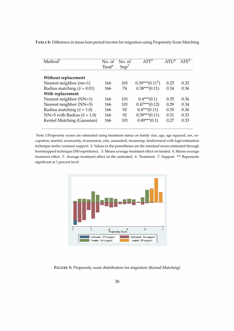
TABLE 8: Difference in mean lean period income for migration using Propensity Score Matching

Method1 No. of No. of ATT3 ATU4 ATE5

Treat6 Sup7

Without replacementNearest neighbor (nn=1) 166 101 0.39***(0.112) 0.25 0.32Radius matching (δ = 0.01) 166 74 0.38***(0.11) 0.34 0.36With replacementNearest neighbor (NN=1) 166 101 0.4***(0.1) 0.35 0.36Nearest neighbor (NN=5) 166 101 0.47***(0.12) 0.29 0.34Radius matching (δ = 1.0) 166 92 0.4***(0.11) 0.35 0.36NN=5 with Radius (δ = 1.0) 166 92 0.39***(0.11) 0.31 0.33Kernel Matching (Gaussian) 166 101 0.49***(0.1) 0.27 0.33

Note 1:Propensity scores are estimated using treatment status on family size, age, age squared, sex, oc-cupation, marital, socsecurity, rivererosion, edu, seasonhrd, mounemp, landownerd with logit estimationtechnique under common support. 2: Values in the parentheses are the standard errors estimated throughbootstrapped technique (500 repetitions). 3: Means average treatment effect on treated. 4: Means averagetreatment effect. 5: Average treatment effect on the untreated. 6: Treatment. 7: Support. *** Representssignificant at 1 percent level.

FIGURE 3: Propensity score distribution for migration (Kernel Matching)

38

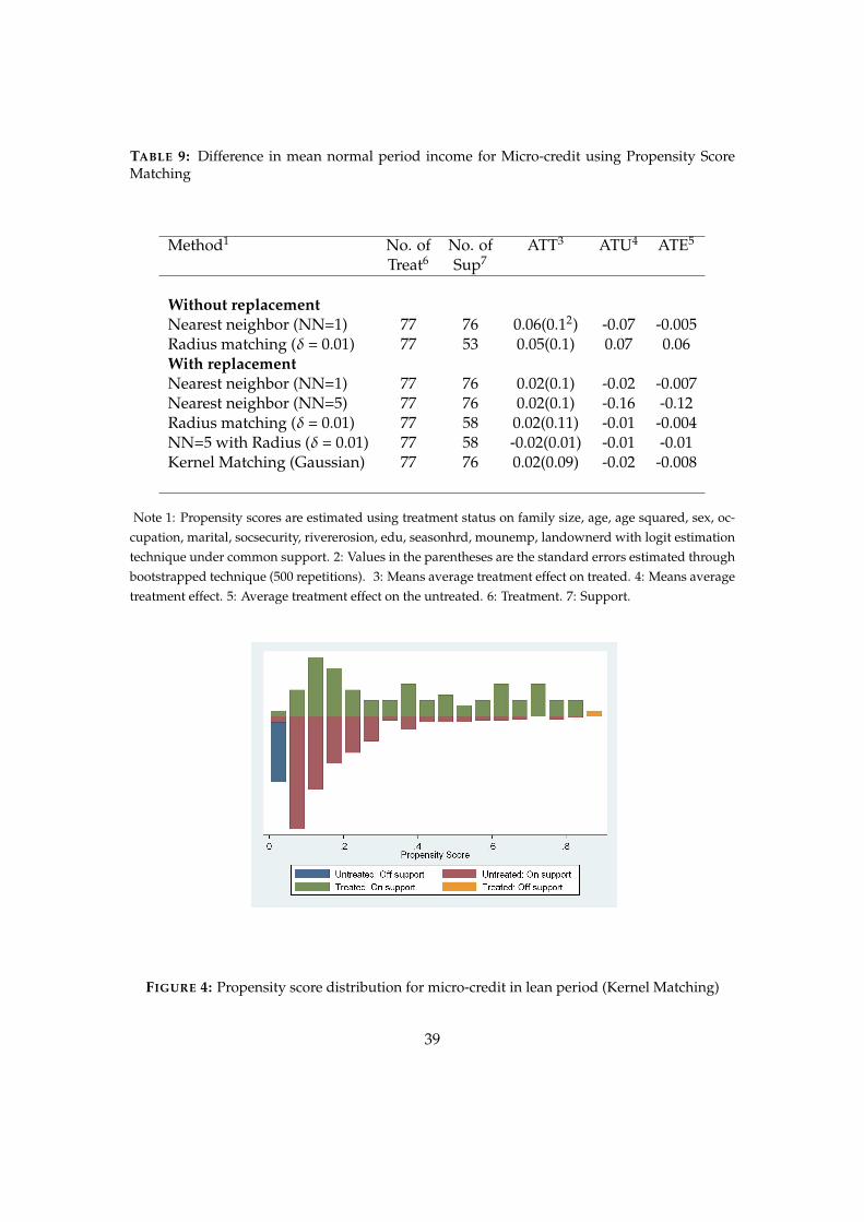
TABLE 9: Difference in mean normal period income for Micro-credit using Propensity ScoreMatching

Method1 No. of No. of ATT3 ATU4 ATE5

Treat6 Sup7

Without replacementNearest neighbor (NN=1) 77 76 0.06(0.12) -0.07 -0.005Radius matching (δ = 0.01) 77 53 0.05(0.1) 0.07 0.06With replacementNearest neighbor (NN=1) 77 76 0.02(0.1) -0.02 -0.007Nearest neighbor (NN=5) 77 76 0.02(0.1) -0.16 -0.12Radius matching (δ = 0.01) 77 58 0.02(0.11) -0.01 -0.004NN=5 with Radius (δ = 0.01) 77 58 -0.02(0.01) -0.01 -0.01Kernel Matching (Gaussian) 77 76 0.02(0.09) -0.02 -0.008

Note 1: Propensity scores are estimated using treatment status on family size, age, age squared, sex, oc-cupation, marital, socsecurity, rivererosion, edu, seasonhrd, mounemp, landownerd with logit estimationtechnique under common support. 2: Values in the parentheses are the standard errors estimated throughbootstrapped technique (500 repetitions). 3: Means average treatment effect on treated. 4: Means averagetreatment effect. 5: Average treatment effect on the untreated. 6: Treatment. 7: Support.

FIGURE 4: Propensity score distribution for micro-credit in lean period (Kernel Matching)

39

TABLE 10: Standardized bias(SB) before and after matching for different matching algorithms

Migration Micro-creditMatching algorithms biased1 biased biased biased

before after before after

Without replacementNearest neighbor (NN=1) 25.22 41.66 21.89 61.81Radius matching (δ = 0.01) 25.22 12.3 21.89 17.64With replacementNearest neighbor (NN=1) 25.22 11.65 21.89 6.72Nearest neighbor (NN=5) 25.22 7.65 21.89 7.47Radius matching (δ = 0.01) 25.22 11.18 21.89 9.92NN=5 with Radius (δ = 0.01) 25.22 11.07 21.89 13.2Kernel Matching (Gaussian) 25.22 5.16 21.89 6.24

Note 1: Following Rosenbaum and Rubin (1985) and Caliendo et al. (2005), for each covariates X it isdefined as the difference of sample means in the treated and matched control sub-samples as a percentageof the square root of the average of sample variances in both groups. The SB before the matching is given

by SBbe f ore = 100( XT−XC√0.5(VT(X)+VC(X))

); SBa f ter = 100(XT|M−XC|M√

0.5(VT|M(X)+VC|M(X))); where XT(VT(X)) is the

mean (variance) in the treatment group before matching and XC(VC(X)) is the same for control group.XT|M(VT|M(X)) and XC|M(VC|M(X)) are the corresponding values for the matched samples.

TABLE 11: Some summary statistics of income in normal period

Normal Periodwithout NGO support with NGO support

Mean 59.63 67.95Median 60 60SD 19.64 23.28Min 20 50Max 120 150

40

TABLE 12: Sensitivity analysis of unobserved heterogeneity for migration

Hodges-Lehman point estimateseγ p-value1+ p-value− t-hat+ t-hat− CI2

1 0.00000 0.00000 0.45814 0.45814 0.30-0.601.1 0.00000 0.00000 0.42364 0.48785 0.29-0.621.2 0.00000 0.00000 0.39992 0.51082 0.23-0.641.3 0.00002 0.00000 0.36698 0.53941 0.21-0.681.4 0.00008 0.00000 0.34657 0.56793 0.18-0.691.5 0.00024 0.00000 0.33533 0.58156 0.16-0.711.6 0.00061 0.00000 0.30306 0.60198 0.14-0.741.7 0.00134 0.00000 0.28768 0.60617 0.12-0.751.8 0.00267 0.00000 0.25541 0.63425 0.10-0.781.9 0.00491 0.00000 0.23500 0.64046 0.74-0.802.0 0.00841 0.00000 0.23500 0.66087 0.05-0.81

Note 1: Reported P-values are the Wilcoxon sign-rank test of significance under hidden bias. Resultsbased on stata ado routine “rbounds”. Calculation is done based on Rosenbaum bounds for ATT; nearestneighbor (1) matching with common support. The outcome variable is the log of income. “+”(“−”) reportsthe results for positive (negative) selection on unobservables. 2: Confidence Interval.

TABLE 13: Some Summary statistics of Income in lean period

Lean PeriodNGO=0,Migdec=0 NGO=0,Migdec=1

Mean 16.17 77.16Median 20 75SD 13.16 38.80Min 0 5Max 50 200

NGO=1,Migdec=1 NGO=1,Migdec=0Mean 74.85 22.72Median 80 25SD 37.18 9.47Min 10 0Max 200 50

41

TABLE 14: Variable description

Name Description VariableMigration decision A dummy variable that equals one if the

individual migrated in one of the last twolean seasons and zero otherwise.

migdec

Income in the leanperiod

Earnings of the household if the chiefearner stayed in the village in the lean pe-riod or the earnings of the household ifthe chief bread-earner migrates in the leanperiod (per day in Local Currency Units,LCU).

mincomelean

Seasonal unemploy-ment

A dummy variable that equals one if theworker remains unemployed during mostof the lean season, zero otherwise.

mounemp

Seasonal hardship A dummy variable that equals one if the in-dividual has one meal or less on a typicalday in the lean period, zero otherwise.

season hrd

Land ownership A dummy variable that equals one if the re-spondent’s family owns any land irrespec-tive of the size of land, zero otherwise.

landownerd

Access to Micro-credit

A dummy variable, which is coded as onefor having access to Micro-credit throughany NGOs, zero otherwise.

ngo

River erosion A dummy variable, such that an individualhas a value of one if his/her family everexperienced forced displacement by rivererosion, zero otherwise.

rivererosion

Flood A dummy variable that equals one if the re-spondent faced flood in the year of migra-tion, and zero otherwise.

flood

Age Actual age of the respondent. ageSex Sex is coded as one if the respondent is

male and zero if she is female.sex

Marital status A dummy variable, coded as one for thosewho are married and zero otherwise.

marital

Education A dummy variable, coded as one for thosewho have any education, zero otherwise.

edu

Household size Number of family members familyFarm occupation A dummy variable, coded as one for the

farmers, zero otherwise.occupationdum

Continued on next page

42

Table 14 – continued from previous pageName Description Variable

Kinship at the placeof destination

A dummy variable, coded as one for thosewho have kinsmen at the potential place ofdestination, zero otherwise.

knship

Migration experience A dummy variable, coded as one for thosewho have prior migration experience (anyprevious experience), zero otherwise.

migexp

Social security A dummy variable, equals one for thosewho reported to receiving any transfer pay-ment from the government, zero otherwise.

sossecurity

43

seasonal migration and the effectiveness of micro-credit...

Documents