T h e A s t r o p h y s i c a l J o u r n a l , 760:53 (lOpp), 2012 November 20 © 2012. The American Astronomical Society. All rights reserved. Printed in the U.S.A.

doi : 10.1088/0004-63 7X/760/1/5 3

SEARCH FOR COSMIC NEUTRINO POINT SOURCES WITH FOUR YEARS OF DATAFROM THE ANTARES TELESCOPE

S. A d r iá n -M a r t ín e z 1 , 1. A l S a m a r a e2, A . A l b e r t 3, M . A n d r é 4, M . A n g h in o l f i5, G . A n t o n 6, S . A n v a r 7, M . A r d id 1,T . A s t r a a t m a d ja 8-39, J -J . A etbert2, B . B a r e t 9, S . B a s a 1", V . B e r t in 2, S . B ia g i1112, C . B ig o n g ia r i13, C . B o g a z z i8,

M . B o u -C a b o 1, B . B o u h o u 9, M . C . B o u w h e t is8, J . B r et n n er2, J . B etsto2, A . C a p o n e 1415, C . C â r l o g a n e t16, J . C a r r 2,S. C e c c h in i11, Z . C h a r if 2, P h . C h a r v is 17, T . C h ia r etsi11, M . C ir c e l l a 18, R . C o n ig l io n e 19, L . C o r e 2, H . C o s t a n t in i2,

P . C o y l e 2, A . C r e u s o t 9, C . C u r t il 2, G . D e B o n is 1415, M . P . D e c o w s k i8, I. D e k e y s e r 2", A . D e s c h a m p s 17, C . D is t e f a n o 19,C . D o n z a u d 9,21, D . D o r n i c 2 1 3 , Q . D o r o s t i 22, D . D r o u h i n 3, T . E b e r l 6, U. E m a n u e l e 13, A . E n z e n h ö f e r 6, J -P . E r n e n w e i n 2,

S . E s c o f f i e r 2, K . F e h n 6, P . F e r m a n i 1415, M . F e r r i 1, S . F e r r y 23, V . F l a m i n i o 24-25, F . F o l g e r 6, U. F r i t s c h 6, J -L . F u d a 2",S. G a l a t à 2, P . G a y 16, K . G e y e r 6, G . G ia c o m e l l i1112, V . G io r d a n o 19, A . G l e ix n e r 6, J . P . G ó m e z -G o n z á l e z 13, K . G r a f 6,

G . G u il l a r d 16, G . H a l l e w e l l 2, M . H a m a l 26, H . v a n H a r e n 27, A . J . H e ij b o e r 8, Y . H e l l o 17, J . J . H e r n á n d e z -R e y 13,B . H e r o l d 6, J . H ö ß L 6, C . C . H s u 8, M . d e J o n g 8-39, M . K a d l e r 28, O . K a l e k i n 6, A . K a p p e s 6-4", U. K a t z 6, O . K a v a t s y u k 22,P . K o o u m a n 8-29-3", C . K o p p e r 6-8, A . K o u c h n e r 9, I. K r e y k e n b o h m 28, V . K u l ik o v s k iy 5-31, R . L a h m a n n 6, G . L a m b a r d 13,G . L a r o s a 1, D . L a t t u a d a 19, E . L e o n o r a 32-33, D . L e f è v r e 2", G . L im 8-3", D . L o P r e s t í32-33, H . L o e h n e r 22, S . L o u c a t o s 23,

F . L o u is 7, S . M a n g a n o 13, M . M a r c e l in 1", A . M a r g io t t a 1112, J . A . M a r t ín e z -M o r a 1, A . M e l i6, T . M o n t a r u l i18-34,M . M o r g a n t i24-41, H . M o t z 6, M . N e f f 6, E . N e z r i 1", D . P a l io s e l it is 8, G . E . P a v a l a ç 35, K . P a y e t 23, J . P e t r o v ic 8,

P . P ia t t e l l i19, V . P o p a 35, T . P r a d ie r 36, E . P r e s a n i8, C . R a c c a 3, C . R e e d 8, G . R ic c o b e n e 19, R . R ic h t e r 6, C . R iv iè r e 2,A . R o b e r t 2", K . R o e n s c h 6, A . R o s t o v t s e v 37, J . R u i z -R iv a s 13, M . R u j o i u 35, D . F . E . S a m t l e b e n 8, P . S a p i e n z a 19, J . S c h m id 6,

J. S c h n a b e l 6, J -P . S c h u l l e r 23, F . S c h ü s s l e r 23, T . S e i t z 6, R . S h a n id z e 6, F . S im e o n e 1415, A . S p ie s 6, M . S p u r io 1112,J . J . M . S t e ij g e r 8, T h . S t o l a r c z y k 23, A . S á n c h e z -L o s a 13, M . T a iu t i5-38, C . T a m b u r in i2", A . T r o v a t o 32, B . V a l l a g e 23,

C . V a l l é e 2, V . V a n E l e w y c k 9, M . V e c c h i2, P . V e r n in 23, E . V is s e r 8, S . W a g n e r 6, G . W i j n k e r 8, J . W il m s 28, E . d e W o l f 8-3",H . Y e p e s 13, D . Z a b o r o v 37, J . D . Z o r n o z a 13, a n d J . Z ctñiga13

1 Institut d’Investigació per a la Gestió Integrada de les Zones Costaneres (IGIC) - Universität Politécnica de València. C/Paranimf 1, E-46730 Gandia, Spain2 CPPM, Aix-Marseille Université, CNRS/IN2P3, Marseille, France

3 GRPHE - Institut universitaire de technologie de Colmar, 34 rue du Grillenbreit, BP 50568 - 68008 Colmar, France 4 Technical University of Catalonia, Laboratory of Applied Bioacoustics, Rambla Exposició, E-08800 Vilanova i la Geltrn, Barcelona, Spain

5 INFN - Sezione di Genova, Via Dodecaneso 33,1-16146 Genova, Italy 6 Friedrich-Alexander-Universität Erlangen-Nürnberg, Erlangen Centre for Astroparticle Physics, Erwin-Rommel-Str. 1, D-91058 Erlangen, Germany

7 Direction des Sciences de la Matière - Institut de recherche sur les lois fondamentales de l’Univers - Service d’Electronique des Détecteurs et d’informatique,CEA Saclay, F-91191 Gif-sur-Yvette Cedex, France

8 Nikhef, Science Park, Amsterdam, The Netherlands 9 APC - Laboratoire AstroParticule et Cosmologie, UMR 7164 (CNRS, Université Paris 7 Diderot, CEA, Observatoire de Paris) 10,

rue Alice Domon et Léonie Duquet, F-75205 Paris Cedex 13, France 10 LAM - Laboratoire d’Astrophysique de Marseille, Pôle de l’Étoile Site de Château-Gombert, rue Frédéric Joliot-Curie 38, F -13388 Marseille Cedex 13, France

11 INFN - Sezione di Bologna, Viale Berti-Pichat 6/2,1-40127 Bologna, Italy 12 Dipartimento di Fisica dell’Università, Viale Berti Pichat 6/2,1-40127 Bologna, Italy

13 IFIC - Instituto de Física Corpuscular, Edificios Investigación de Paterna, CSIC - Universität de València, Apdo. de Correos 22085, E-46071 Valencia, Spain14 INFN -Sezione di Roma, P.le Aldo Moro 2,1-00185 Roma, Italy

15 Dipartimento di Fisica dell’Uni versità La Sapienza, P.le Aldo Moro 2,1-00185 Roma, Italy 16 Clermont Université, Université Biaise Pascal, CNRS/IN2P3, Laboratoire de Physique Corpusculaire, BP 10448, F-63000 Clermont-Ferrand, France

17 Géoazur - Université de Nice Sophia-Antipolis, CNRS/INSU, IRD, Observatoire de la Côte d’Azur and Université Pierre et Marie Curie,BP 48, F-06235 Villefranche-sur-mer, France

18 INFN - Sezione di Bari, Via E. Orabona 4,1-70126 Bari, Italy 19 INFN - Laboratori Nazionali del Sud (LNS), Via S. Sofia 62,1-95123 Catania, Italy

20 COM - Centre d’Océanologie de Marseille, CNRS/INSU et Université de la Méditerranée, 163 Avenue de Luminy, Case 901, F-13288 Marseille Cedex 9, France21 Univ Paris-Sud, F-91405 Orsay Cedex, France

22 Kernfysisch Versneller Instituut (KVI), University of Groningen, Zernikelaan 25, 9747 AA Groningen, The Netherlands 23 Direction des Sciences de la Matière - Institut de recherche sur les lois fondamentales de l ’Univers - Service de Physique des Particules,

CEA Saclay, F-91191 Gif-sur-Yvette Cedex, France 24 INFN - Sezione di Pisa, Largo B. Pontecorvo 3,1-56127 Pisa, Italy

25 Dipartimento di Fisica dell’Université, Largo B. Pontecorvo 3,1-56127 Pisa, Italy 26 University Mohammed I, Laboratory of Physics of Matter and Radiations, BP 717, Oujda 6000, Morocco

27 Royal Netherlands Institute for Sea Research (NIOZ), Landsdiep 4,1797 S Z ’t Horntje (Texel), The Netherlands28 Dr. Remeis-Sternwarte and ECAP, Universität Erlangen-Nürnberg, Sternwartstr. 7, D-96049 Bamberg, Germany

29 Universiteit Utrecht, Faculteit Bètawetenschappen, Princetonplein 5, 3584 CC Utrecht, The Netherlands 30 Universiteit van Amsterdam, Instituut voor Hoge-Energie Fysica, Science Park 105, 1098 XG Amsterdam, The Netherlands

31 Moscow State University, Skobeltsyn Institute of Nuclear Physics, Leninskie gory, 119991 Moscow, Russia 32 INFN - Sezione di Catania, Viale Andrea Doria 6,1-95125 Catania, Italy

33 Dipartimento di Fisica ed Astronomía dell’Université, Viale Andrea Doria 6,1-95125 Catania, Italy 34 Département de Physique Nucléaire et Corpusculaire, Université de Genève, 1211, Geneva, Switzerland

35 Institute for Space Sciences, R-77125 Bucharest, Mägurele, Romania 36 IPHC-Institut Pluridisciplinaire Hubert Curien - Université de Strasbourg et CNRS/IN2P3 23 rue du Loess, BP 28, F-67037 Strasbourg Cedex 2, France

37 ITEP - Institute for Theoretical and Experimental Physics, B. Cheremushkinskaya 25, 117218 Moscow, Russia 38 Dipartimento di Fisica dell’Université, Via Dodecaneso 33,1-16146 Genova, Italy

Received 2012 July 12; accepted 2012 October 3; published 2012 November 2

1

T h e A st r o p h y s ic a l J o u r n a l , 760:53 (lOpp), 2012 November 20 A d r iá n -M a r t ín e z e t a l .

ABSTRACT

In this paper, a time-integrated search for point sources of cosmic neutrinos is presented using the data collected from 2007 to 2010 by the ANTARES neutrino telescope. No statistically significant signal has been found and upper limits on the neutrino flux have been obtained. Assuming an E ~2 spectrum, these flux limits are at 1 - I0 x l0 ~ 8 GeV c u r 2 s_1 for declinations ranging from —90° to 40°. Limits for specific models of RX J1713.7 -3 9 4 6 and Vela X, which include information on the source morphology and spectrum, are also given.

Key words: astroparticle physics - cosmic rays - neutrinosOnline-only material: color figures

1. INTRODUCTION

One of the main goals of the ANTARES telescope (Ageron et al. 2011) is the detection of cosmic neutrinos and the identification of their sources. Neutrinos only interact via the weak interaction and are stable, making them unique probes to study the high-energy universe. The production of high-energy neutrinos has been proposed (Halzen & Hooper 2002; Bednarek et al. 2005; Stecker 2005) for several kinds of astrophysical sources in which the acceleration of hadrons may occur. In the interaction of cosmic rays (CRs) with matter or radiation, charged pions are produced. The decay of these charged pions yields neutrinos and muons. The subsequent decay of the latter produces in turn more neutrinos. While CRs, except at ultra high energies, are deflected by galactic and intergalactic magnetic fields, neutrinos point back to their sources. Therefore, the detection of neutrinos may give valuable information on the origin of CRs. It would also settle the question of the hadronic versus leptonic mechanism in several sources from which high- energy gamma rays have been observed (Berezhko et al. 2008).

The best neutrino flux upper limits up to PeV energies for the Southern Hemisphere have been established by the ANTARES experiment using 2007-2008 data (Adrián-Martínez et al. 2011). In the present paper, this analysis is extended by adding two more years of data with the full configuration of 12 detection lines. Furthermore, the information on the amount of light produced in the events, which is a quantity correlated to the neutrino energy and which helps to distinguish the atmospheric neutrino background from a potential high-energy signal, is taken into account.

The structure of this paper is as follows. In Section 2 the ANTARES detector is briefly described. Sections 3 and 4 describe the online selection and the simulation, respectively. The track reconstruction is explained in Section 5. The selection of events is described in Section 6. Section 7 is devoted to the evaluation of the detector performance. The search method and the limit setting are described in Sections 8 and 9. Section 10 shows how the search is improved by including the energy information. Results are presented in Section l l . A cross-check based on an alternative method is explained in Section 12. Finally, the conclusions are summarized in Section 13.

2. THE ANTARES DETECTOR

The operation principle of neutrino telescopes is based on the detection of the Cherenkov light induced by relativistic muons produced in the charged current (CC) weak interactions of high- energy neutrinos close to or inside the detector. The information

39 Also at University of Leiden, the Netherlands.40 On leave of absence at the Humboldt-LTniversität zu Berlin.41 Also at Accademia Navale de Livorno, Livorno, Italy.

on the time and position of the detected photons is used to reconstruct the muon trajectory, which is correlated with the direction of the incoming neutrino. Other signatures are also possible, such as the cascades produced in the CC interactions of electron and tau neutrinos and in the neutral current interactions of all neutrino flavors. In this analysis muons induced by high-energy neutrinos are used. For these events, the detector acceptance is large due to the long muon range and the neutrino direction is derived with an accuracy of a fraction of a degree.

The construction of the ANTARES detector (Ageron et al. 2011) was completed in 2008, after several years of site exploration and detector R&D (Amram et al. 2002; Aguilar et al. 2005a, 201 la). The detector is located at (42°48/ N, 6° 10' E) at a depth of 2475 m, in the Mediterranean Sea, 40 km from the French town of Toulon. It comprises a three-dimensional array of 885 optical modules (OMs) looking 45° downward and distributed along 12 vertical detection lines. An OM (Amram et al. 2002) consists of a 10 inch photomultiplier (PMT) housed in a glass sphere together with its base, a special gel for optical coupling and a //-metal cage for magnetic shielding. The OMs are grouped in 25 triplets (or storeys) on each line, except for one of the lines on which acoustic devices are installed (Aguilar et al. 2011b) and which therefore contains only 20 optical storeys. The total length of each line is 450 m; these are kept taut by a buoy located at the top of the line. The lower 100 m are not instrumented. The distance between triplets is 14.5 m and the separation between the lines ranges from 60 to 75 m. The lines are connected to a central junction box, which in turn is connected to shore via an electro-optical cable. Figure 1 shows a schematic view of the detector.

The detector also includes several calibration systems. The lines slowly move due to the sea current (up to ~ 15 m at the top of the line in case of currents of 20 cm s-1 ). A set of acoustic devices together with tiltmeters and compasses along the lines are used to reconstruct the shape of the lines and orientation of the storeys every two minutes (Adrián-Martínez et al. 2012). The acoustic system provides the position of each optical module with a precision better than 15 cm. The time calibration is performed by means of a master clock on shore and a set of optical beacons (four along each line). This allows for a calibration of the time offsets of the photomultipliers with a precision better than 1 ns (Aguilar et al. 201 la).

In this analysis, data from 2007 January 29 to 2010 November 14 are used. The total integrated live-time is 813 days, out of which 183 correspond to the five-line period. Causes of loss of efficiency are periods of high bioluminescence and sea operations.

3. ONLINE SELECTION

The charge and time information of all signals from the PMTs which exceed a pre-defined threshold voltage, typically the

2

T h e A st r o p h y s ic a l J o u r n a l , 760:53 (lOpp), 2012 November 20 A d r iá n -M a r t ín e z e t a l .

buoy Q electronics container

optical modules

ñ

' i o

40 km cable to shore

junctionboxseabed

Figure 1. Schematic view of the ANTARES detector, consisting of 12 mooring lines connected to the shore station through an electro-optical cable.(A color version of this figure is available in the online journal.)

equivalent to 0.3 single photoelectrons (Aguilar et al. 2007), are first digitized into "hits" and then sent to shore where they are filtered by a farm of PCs. For this analysis, two different filter algorithms were used to select the events. Both are based on the assumption that the optical background processes such as potassium-40 radioactive decays and bioluminescence are not correlated and induce single photoelectron hits. Hence, a first selection of the signal requires hits with a high charge (usually >3 photoelectrons) or coincident hits within a time window of 20 ns on separate OMs of the same storey (LI hits). The first trigger requires at least five L Í hits compatible with a muon track in any direction. The second trigger is defined as the occurrence of at least two LÍ hits in three consecutive storeys within a specific time window. This time window is 100 ns in the case where the two storeys are adjacent and 200 ns for next-to-adjacent storeys. In addition to the events selected by the trigger, the singles count rate of each OM is stored.

4. SIMULATIONS

Simulations are required for determining the acceptance and angular resolution of the detector, since in the absence of a source these quantities cannot readily be measured.

The event simulation starts with the generation of upgoing muon neutrino events using the GENHEN package (Bailey 2002), which uses CTEQ6D (Pumplin et al. 2002) parton density functions for computing the deep inelastic charged current neutrino scattering cross section. The events are weighted according to the cross section and their probability to survive the passage through the Earth. If the neutrino interaction occurs near the detector, the hadronic shower resulting from the break-up of the target nucleon is simulated using GEANT (Brunner 2003). Otherwise, only the resulting muon is propagated to the detector using the MUSIC code (Antonioli et al. 1997). Atmospheric muons reconstructed as upgoing are a source of background for a neutrino signal and their rejection is a crucial point in this analysis as will be described in Section 6. Downgoing atmospheric muons were simulated with the program MUPAGE (Carminati et al. 2008; Becherini et al. 2006) which provides parameterized muons and muon bundles at the detector.

Inside the detector, the Cherenkov photons emitted along a muon track and arriving on the OMs are simulated by sampling

tabulated values of photon arrival times. The arrival time distributions have been derived by tracking individual photons taking into account the measured absorption and scattering parameters (Aguilar et al. 2005b).

The PMT transit time spread (TTS ) is simulated by a Gaussian smearing of photon arrival times. Optical backgrounds are added to the events according to the measured rates observed in the count rate data. Similarly, simulated hits from inactive OMs are deleted from the event. Sampling the count rate data from the runs selected for the analysis ensures that the simulation contains the same background and detector conditions as the analyzed data set. The same trigger algorithms are applied to the simulation and the data.

An uncertainty of 50% on the atmospheric muon flux is es­timated using the same procedure described in Aguilar et al. (2010). For the atmospheric neutrino flux, a systematic uncer­tainty of 30% is considered (Barr et al. 2006).

5. RECONSTRUCTION

Tracks are reconstructed from the hits in the triggered events using a multi-step algorithm (see Heijboer 2004 for a more detailed description). The initial steps provide a starting point for the final maximization of the track likelihood. The likelihood is defined as the probability density of the observed hit time residuals, r, given the track parameters (position at some arbitrary time and direction). The time residual r is defined as the difference between the observed and expected hit time for the assumed track parameters.

It was found that the likelihood function has many local maxima and that the maximization procedure needs to be started with track parameters close to the optimal values. The initial steps in the algorithm provide this near-optimal solution, estimating the track parameters using increasingly refined score functions: a linear x 2 fit, a so-called M-estimator minimizing g(r) = s / l + r2 and a simplified version of the full likelihood fit. Each fit uses increasingly more inclusive hit selections based on the preceding stage. This sequence is started at nine different starting points to further increase the probability of finding the global optimum. Using more than nine starting points was found to have only marginal impact on the reconstruction quality and was not deemed worth the additional processing time.

The final likelihood function uses parameterizations for the probability density function (pdf) of the signal hit time residual, derived from simulations. The pdfs also include hits arriving late due to Cherenkov emission by secondary particles or light scattering. Furthermore, the probability of a hit being due to background is accounted for.

The quality of the track fit is quantified by the parameter

A = log(¿)Mats - 5

+ 0.1 x (iVcomp — 1), ( 1)

which incorporates the maximum value of the likelihood, L, and the number of degrees of freedom of the fit, i.e., the number of hits, (Vhits, used in the fit minus the number of fit parameters; Ncomp is the number of times the repeated initial steps of the re­construction converged to the same result. In general, N comp = 1 for badly reconstructed events while it can be as large as nine for well reconstructed events. The coefficient 0.1 in Equation (1) was chosen to maximize the separation in A between simulated signal and misreconstructed downgoing muons.

The A variable can be used to reject badly recon­structed events, in particular atmospheric muons that are

3

T h e A st r o p h y s ic a l J o u r n a l , 760:53 (lOpp), 2012 November 20 A d r iá n -M a r t ín e z e t a l .

Table 1Number of Events before and after Applying Selection Cuts for Data (Second Column) and Monte Carlo Simulations (Third, Fourth, and Fifth Columns)

Data Atm. ¡i Atm. V E ~2v

Triggered events 3.94 x IO8 3.06 x IO8 1.54 x IO4 100%

Reco. upgoing events 6.08 x IO7 2.98 x IO7 1.24 x IO4 61%

Reco. upgoing events + ß < 1° 3.90 x IO7 1.57 x IO7 8352 44%

Reco. upgoing + ß < 1° + A > —5.2 3058 358 2408 23%

Notes. The last column shows the percentage of signal events assuming a neutrino flux proportional to an E v ~ spectrum.

: 10' • data— V MC— Ii MC

o

IQ-

10

0 2 4 6ß (degrees)

Figure 2. Distribution of the estimate of the error on the direction of the reconstructed upgoing muon track after applying a cut on the quality variable A > —5.2. The red line shows the Monte Carlo atmospheric neutrinos, the purple line the Monte Carlo misreconstructed atmospheric muons and the black dots the data. The vertical dashed line with the arrow shows where the selection cutis applied ( ß < Io).(A color version of this figure is available in the online journal.)

datao 10'

10

10

10"10'

0.5-7 -6.5 -6 -5.5 -5 -4.5 -4

quality variable A

Figure 3. Cumulative distribution of the reconstruction quality variable A for upgoing tracks which have an angular error estimate ß < Io. The bottom panel shows the ratio between data and simulations. The red line is for Monte Carlo atmospheric neutrinos, the purple line Monte Carlo misreconstructed atmospheric muons and the black dots the data. The vertical dashed line with the arrow shows where the selection cut is applied (A > —5.2). The purple and red bands show the systematic uncertainties on the simulations as explained in Section 4. The green band in the bottom panel shows the total contribution of these uncertainties.(A color version of this figure is available in the online journal.)

misreconstructed as upgoing. In addition, assuming that the likelihood function near the fitted maximum follows a multivari­ate Gaussian distribution, the error on the zenith and azimuth angles are estimated from the covariance matrix. The angular uncertainty on the muon track direction, ß, is obtained from these errors and can be used to further reject misreconstructed atmospheric muons as discussed in Section 6.

6. EVENT SELECTION

Neutrino candidates are selected requiring tracks recon­structed as upgoing and applying selection criteria. These cri­teria were chosen following a "blind" procedure, i.e., before performing the analysis on data. The effect of the selection cuts on data, expected background and signal efficiency are summarized in Table 1.

The estimated angular uncertainty on the muon track direc­tion, ß, is required to be smaller than 1 deg. This cut rejects 47% of the atmospheric muons which are misreconstructed as upgoing tracks.

To further reject atmospheric muons that were misrecon­structed as upgoing, the quality variable A is required to be larger than -5 .2 . This value is chosen to optimize the discovery potential, i.e., the neutrino flux needed to have a 50% chance of discovering the signal at the 5a significance level assuming an E ~2 spectrum.

Figure 2 shows the distribution of ß for upgoing events with A > -5 .2 . The cumulative distribution of A for upgoing events is shown in Figure 3. The cut on the angular error estimate ß is also applied. The excess of data compared to simulations at the lowest values of A is due to a non-simulated contribution of events consisting of solely optical background. Figure 4 shows the distribution of the reconstructed cosine of the zenith angle for both data and simulation.

The final sample consists of 3058 neutrino candidate events out of a total of ~ 4 x IO8 triggered events. Simulations predict 358 ± 1 7 9 atmospheric muons and 2408 ± 722 atmospheric neutrinos, yielding a total expected events of 2766 ± 743. This is consistent with the observed rate within the quoted uncertainties (see Section 4).

7. DETECTOR PERFORMANCE

The response of the detector to a neutrino signal proportional to an E ~2 spectrum was obtained using the simulation described in Section 4 and applying the analysis cuts.

7.1. Angular Resolution

Figure 5 (left) shows the cumulative distribution of the angle between the direction of the reconstructed muon and that of the true neutrino. The median of this distribution is 0.46 ± 0.10 deg. Of the selected events, 83% are reconstructed better than 1 deg.

4

T h e A s t r o p h y s i c a l J o u r n a l , 760:53 (lOpp), 2012 November 20 A d r iá n -M a r t ín e z e t a l .

oo — data V MC pM C

«co>o

occ

0.2 0.4 0.6 0.8 1cos(zenith angle)

Figure 4. Distribution of the cosine of the zenith angle showing events with A > —5.2 and ß < Io. The bottom panel shows the ratio between data and the total contribution of simulations. The simulated distributions are shown for atmospheric muons and neutrinos. Systematic uncertainties on Monte Carlo atmospheric muons and neutrinos are shown by the purple and red bands, respectively. The green band corresponds to the sum of these uncertainties. The vertical dashed line with the arrow shows where the cut on the zenith angle is applied in order to select only upgoing events.(A color version of this figure is available in the online journal.)

For the data sample in which the detector was operational with all 12 lines, the estimated angular resolution is 0.43 ± 0.10 deg. The median of this angular error for the full data set considered in the analysis is shown in Figure 5 (right) as a function of the true neutrino energy.

The systematic uncertainty on the angular resolution quoted above has been estimated by varying the hit time resolution, Aí, in the simulation. Many possible effects can contribute to this resolution, including the PMT transit time spread, miscalibra- tions of the timing system and possible spatial misalignments of the detector. The hit time resolution directly impacts both the angular resolution and the number of events passing the quality criteria. Simulations using different Aí values were compared with data in order to determine the best agreement in the lambda distribution, and was obtained for Aí = 2.5 ns. This can be compared to the TTS of the PMT, which is 1.3 ns (standard deviation). Fiowever, the PMT time response is not Gaussian and the degraded resolution was found to partly account for the tails. A Aí of 2.5 ns yields the quoted angular resolution of 0:46 and is the value used in the plots shown in this paper.

For Aí = 3.4 ns, the simulations show a deterioration in angular resolution of 30% and the number of selected neutrino events in the data exceeds the simulated neutrino signal by 2a, where a refers to the uncertainty on the atmospheric neutrino flux model. Hence, this value of Aí is excluded from the data. Assuming a linear dependency, this argument translates to a (1er) uncertainty on the angular resolution of ~15% .

The absolute orientation of the detector is known with an accuracy of ~ 0 i l (Adrián-Martínez et al. 2012).

7.2. Acceptance

The neutrino effective area, A ,ff, is defined as the ratio between the neutrino event rate, R V(E V), and the cosmic neutrino flux, 4>(£v). The flux is assumed to consist of equal amounts of Vfi and Vfi. The neutrino effective area depends on the neutrino cross section, the absorption of neutrinos through the Earth and the muon detection (and selection) efficiency. It can be

0.4

0.2

10angle (degrees)

Co3OV)<Di-jo 13U)C 0.8cic

.5 0.6■Oa)£ 0.4

°-22L 2.5 3.5 4.5 5.5 6.5l.o U U.O I

log10(E /G eV )

Figure 5. Top: cumulative distribution of the angle between the reconstucted muon direction and the true neutrino direction for upgoing events of the whole data set. A neutrino spectrum proportional to E~2 is assumed. Bottom: the median angle as a function of the neutrino energy Ev. In these plots the cuts A > —5.2 and ß < Io are applied.

considered as the equivalent area of a 100% efficient detector. Figure 6 shows the effective area as a function of the neutrino energy and declination, Sv.

The analysis is primarily concerned with cosmic sources emitting neutrinos with an E~2 power law of the form

d N v ( E v V 2 i t i 1— = ó x [ — — I GeV cm s , (2)d E y d td S * \G eV /

where the constant <f> is the flux normalization. The acceptance, A(SV), for such a flux, is defined as the constant of proportional­ity between <f> and the expected number of events in the source direction and can be expressed in terms of the effective area as

A{8v) = <f>~1 j j d t d E vA f ( E v, S v) J ^ . (3)

The acceptance for this analysis is shown in Figure 6 (bottom). For a source at a declination of -90(0)°, A = 8.8(4.8) x IO7 GeV-1 cm2 s which means that a total of 8.8(4.8) neutrino candidates would be selected from a point-like source emitting a flux of 1(T7 x ( E J G e V r 2 GeV^1 cm ^2 s“ 1.

5

T h e A s t r o p h y s i c a l J o u r n a l , 760:53 (lOpp), 2012 November 20 A d r iá n -M a r t ín e z e t a l .

-90 < Ô < -45 -45° < ô < 0°10

1

2 2.5 3 3.5 4 4.5 5 5.5 6 6.5 7logio(E v/G eV )

9

8

7

6

5

4

3

2

1

0■1 -0.8 -0.6 -0.4 -0.2 0 0.2 0.4 0.6 0.8 1

sin(8)

Figure 6. Top: the neutrino effective area for the selected events as a function of the neutrino energy Ev for three different declination bands. Bottom: acceptance of the detector which is proportional to the number of events that would be detected and selected from a point-like source at a given declination assuming a flux of IO-7 x (Ev/G eV )~2 GeV-1 cm-2 s-1 as a function of the sine of the declination.(A color version of this figure is available in the online journal.)

To constrain the systematic uncertainty on the acceptance, a comparison between the atmospheric neutrino data and a simulation was performed in which the efficiency of each of the OMs was reduced by 15%, which yields a 12% reduction of the signal events for an E ~2 flux. The atmospheric neutrino yield would instead be reduced by 40% to be compared to the 30% error on its flux normalization. Therefore, the 15% uncertainty on the acceptance can be therefore considered a conservative choice.

8. SEARCH METHOD

Two alternative searches for point-like neutrino sources have been performed. The full-sky search looks for an excess of signal events over the atmospheric muon and neutrino backgroundanywhere in the visible sky, i.e., in the declination range (—90°, +48°). In the candidate list search, the presence of an excess of events is tested at the locations of the 51 pre­defined candidate sources given in Table 2. They include the 24 source candidates from Adrián-Martínez et al. (2011) and 27 new sources selected considering their gamma-ray flux and their visibility at the ANTARES site as the selection criteria. Among the Galactic sources only TeV gamma-ray emitters are considered. No such requirement is imposed for

= io­ns — dat a atm . p + atm . v

-Q<0-QO* 10

20 40 60 80 100 120 140 160 180 200number of hits

Figure 7. Distribution of the number of hits used in the reconstruction, for the selected data (black dots), and the total Monte Carlo background contribution, i.e., atmospheric muons and atmospheric neutrinos (solid green line). The dashed blue line corresponds to the cosmic neutrino signal assuming an E ~2 spectrum. The distribution is normalized to the integral of the total number of events. All the cuts described in Section 6 are applied.(A color version of this figure is available in the online journal.)

extragalactic sources as TeV gamma rays may be absorbed by the extragalactic background light (Nikishov 1962; Gould et al. 1966; Jelley 1966).

The algorithm for the cluster search uses an unbinned maximum likelihood (Barlow 1990) which is defined as

log £ s+b = E 1o8 k s x •r (V'7(Q's, 5S)) x AT(iV¿ts)i

+ B(8j) x AAbg (N U ) ] - / j s - Mbg, (4)

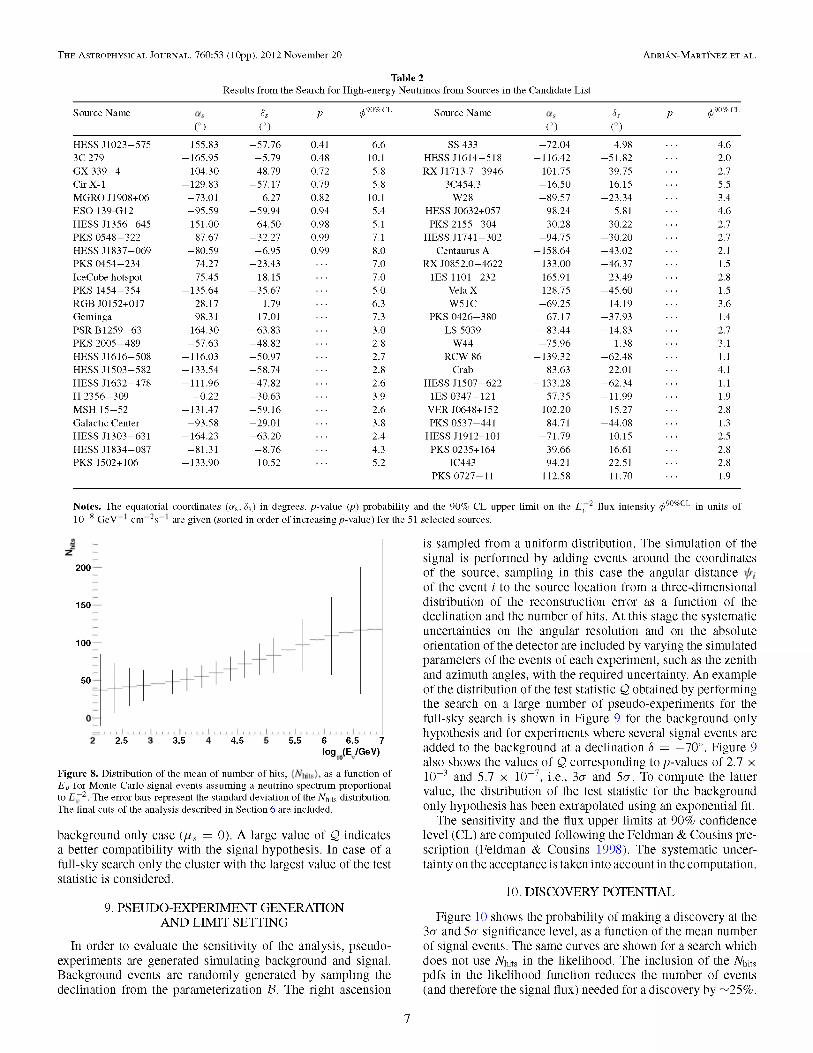
where the sum is over the events; T is a parameterization of the point spread function, i.e., the probability density function of reconstructing event i at an angular distance i/'t from the true source location (as, 5S); B is a parameterization of the background rate obtained from the distribution of the observed declination of the 3058 selected events; / /s and //bg are the mean number of signal events and the total number of expected background events; V¿its is the number of hits used in the reconstruction. N 's(N¡íits) and A/’bg(iV its) are the probabilities of measuring N¡¿ts hits for signal and background, respectively. The distribution of N¡¿ts for data and Monte Carlo events is shown in Figure 7. Figure 8 shows the distribution of Nuts for signal as a function of the true neutrino energy.

In the candidate list search, the sum in Equation (4) incorpo­rates the events located in a cluster within 20 deg of the source. Events further away have T ~ 0 and thus contribute a constant factor to the likelihood. In the full-sky search potentially signif­icant clusters are first identified by selecting at least four events within a eone of 3 deg diameter. Using a larger diameter or a bigger/lower number of required events increases the computa­tion time without a significant improvement in the sensitivity.

In the candidate list search the likelihood is maximized by numerically fitting the mean number of signal events, \is, with the source location fixed. In the full-sky search the likelihood maximization yields the source coordinates and ß s for each cluster. After likelihood maximization a test statistic, Q, is computed:

Q = log £ ” abx - log £ b, (5)where log is the maximum value of the likelihood provided by the fit and lo g £ b is the likelihood computed for the

6

T h e A st r o p h y s ic a l J o u r n a l , 7 6 0 :5 3 (lOpp), 2 0 1 2 November 2 0 A d r iá n -M a r t ín e z e t a l .

Table 2Results from the Search for High-energy Neutrinos from Sources in the Candidate List

Source Namen

Ssn P

090% CL Source Namen

Ssn P

090% CL

HESS J1023—575 155.83 -5 7 .7 6 0.41 6.6 SS 433 -7 2 .0 4 4.98 4.63C 279 -165 .95 -5 .7 9 0.48 10.1 HESS J1614—518 -1 1 6 .4 2 -5 1 .8 2 2.0GX 3 3 9 -4 -1 0 4 .3 0 -4 8 .7 9 0.72 5.8 RX J1713.7—3946 -101 .75 -3 9 .7 5 2.7CirX -1 -129 .83 -5 7 .1 7 0.79 5.8 3C454.3 -1 6 .5 0 16.15 5.5MORO J 1908+06 -73 .01 6.27 0.82 10.1 W28 -8 9 .5 7 -2 3 .3 4 3.4ESO 139-G12 -9 5 .5 9 -5 9 .9 4 0.94 5.4 HESS J0632+057 98.24 5.81 4.6HESS J1356—645 -1 5 1 .0 0 -6 4 .5 0 0.98 5.1 PKS 2155-304 -3 0 .2 8 -3 0 .2 2 2.7PKS 0548-322 87.67 -3 2 .2 7 0.99 7.1 HESS J1741—302 -9 4 .7 5 -3 0 .2 0 2.7HESS J1837—069 -8 0 .5 9 -6 .9 5 0.99 8.0 Centaurus A -1 5 8 .6 4 -4 3 .0 2 2.1PKS 0454-234 74.27 -2 3 .4 3 7.0 RX J0852.0 —4622 133.00 -4 6 .3 7 1.5IceCube hotspot 75.45 -1 8 .1 5 7.0 1ES 1101-232 165.91 -2 3 .4 9 2.8PKS 1454-354 -1 3 5 .6 4 -3 5 .6 7 5.0 V elaX 128.75 -4 5 .6 0 1.5RGB J0152+017 28.17 1.79 6.3 W51C -6 9 .2 5 14.19 3.6Geminga 98.31 17.01 7.3 PKS 0426 -3 8 0 67.17 -3 7 .9 3 1.4PSR B1259—63 -1 6 4 .3 0 -6 3 .8 3 3.0 LS 5039 -8 3 .4 4 -1 4 .8 3 2.7PKS 2005-489 -5 7 .6 3 -4 8 .8 2 2.8 W44 -7 5 .9 6 1.38 3.1HESS J1616—508 -116 .03 -5 0 .9 7 2.7 R C W 86 -1 3 9 .3 2 -6 2 .4 8 1.1HESS J1503—582 -1 3 3 .5 4 -5 8 .7 4 2.8 Crab 83.63 22.01 4.1HESS J1632—478 -1 1 1 .9 6 -4 7 .8 2 2.6 HESS J1507—622 -1 3 3 .2 8 -6 2 .3 4 1.1H 2 356-309 -0 .2 2 -3 0 .6 3 3.9 1ES 0347-121 57.35 -1 1 .9 9 1.9MSH 1 5 -5 2 -1 3 1 .4 7 -5 9 .1 6 2.6 VER J0648+152 102.20 15.27 2.8Galactic Center -9 3 .5 8 -29 .01 3.8 PKS 0537-441 84.71 -4 4 .0 8 1.3HESS J1303—631 -164 .23 -6 3 .2 0 2.4 HESS J 1912+101 -7 1 .7 9 10.15 2.5HESS J1834—087 -81 .31 -8 .7 6 4.3 PKS 0235+164 39.66 16.61 2.8PKS 1502+106 -1 3 3 .9 0 10.52 5.2 IC443

PKS 0 727-1194.21

112.5822.5111.70

2.81.9

Notes. The equatorial coordinates (a's, Ss) in degrees, p -value (p) probability and the 90% CL upper limit on the E v 2 flux intensity ¡j>90%CL m units of 10~8 GeV cm es are given (sorted in order of increasing p - value) for the 51 selected sources.

is sampled from a uniform distribution. The simulation of the signal is performed by adding events around the coordinates of the source, sampling in this case the angular distance of the event i to the source location from a three-dimensional distribution of the reconstruction error as a function of the declination and the number of hits. At this stage the systematic uncertainties on the angular resolution and on the absolute orientation of the detector are included by varying the simulated parameters of the events of each experiment, such as the zenith and azimuth angles, with the required uncertainty. An example of the distribution of the test statistic Q obtained by performing the search on a large number of pseudo-experiments for the full-sky search is shown in Figure 9 for the background only hypothesis and for experiments where several signal events are added to the background at a declination S = —70°. Figure 9 also shows the values of Q corresponding to p-values of 2.7 x IO-3 and 5.7 x 1(U7, i.e., 3a and 5a. To compute the latter value, the distribution of the test statistic for the background only hypothesis has been extrapolated using an exponential fit.

The sensitivity and the flux upper limits at 90% confidence level (CL) are computed following the Feldman & Cousins pre­scription (Feldman & Cousins 1998). The systematic uncer­tainty on the acceptance is taken into account in the computation.

200

150

100

50

2.5 3.5 4.5 5.5 6 6.5 7lo g JE /G eV )

Figure 8. Distribution of the mean of number o f hits, as a function ofE v for M onte Carlo signal events assuming a neutrino spectrum proportional to E ~ 2 . The error bars represent the standard deviation of the A^its distribution. The final cuts of the analysis described in Section 6 are included.

background only case (jus = 0). A large value of Q indicates a better compatibility with the signal hypothesis. In case of a full-sky search only the cluster with the largest value of the test statistic is considered.

9. PSEUDO-EXPERIMENT GENERATION AND LIMIT SETTING

In order to evaluate the sensitivity of the analysis, pseudo­experiments are generated simulating background and signal. Background events are randomly generated by sampling the declination from the parameterization B. The right ascension

10. DISCOVERY POTENTIAL

Figure 10 shows the probability of making a discovery at the 3a and 5a significance level, as a function of the mean number of signal events. The same curves are shown for a search which does not use N^its in the likelihood. The inclusion of the Nuts pdfs in the likelihood function reduces the number of events (and therefore the signal flux) needed for a discovery by ~25% .

7

T h e A st r o p h y s ic a l J o u r n a l , 760:53 (lOpp), 2012 November 20 A d r iá n -M a r t ín e z e t a l .

1 background only 3 signal events 6 signal events -9 signal events

i So3o

IO'1

0 20 40 60Q

Figure 9. Distribution of the test statistic Q for the full-sky search. The full yellow histogram is for the background only experiments. The red, blue, and green lines are for 3, 6, and 9 signal events generated from a source with an E~2 spectrum at a declination of —70°. The vertical dotted lines show the values of Q corresponding to the 3a and 5a significance level.(A color version of this figure is available in the online journal.)

The worsening of the 3a and 5a discovery probability for a neutrino flux model with an exponential cutoff parameterized as d N / d E = <p x (£j,/G eV )-2 exp( - E v/ E c), with Ec the cutoff energy, was estimated. In this case, for a source at a declination of 5 = —70°, the mean number of signal events needed for a 5a discovery assuming a cutoff energy E c = 1 TeV is a factor 2 higher compared to that without an exponential cutoff.

Simulations show that for a source with Gaussian extension resource = 1° at a declination of 5 = —70°, the flux needed to claim a 5a discovery is a factor 1.2 higher compared to a point-like source.

11. RESULTS

A map in equatorial coordinates of the pre-trial significances of every point in the sky that is visible below the horizon at the ANTARES site is shown in Figure 11.

In the full-sky search the most significant cluster is located at (a, 8) = ( -4 6 :5 , -6 5 :0 ), where 5(9) events are within 1(3) deg of this position. For this cluster the fit assigns 5.1 as signal events, and the value of the test statistic is Q = 13.1. The corresponding p-value is obtained by comparing the value of the observed test statistic Q with the simulated Q distribution for the background only hypothesis. The post-trial p-value is 2.6%, which is equivalent to 2.2a (using the two-sided convention).

The results from the search up the 51 a priori selected candidate sources are presented in Table 2 and shown in Figure 12. The most signal-like candidate source in the list is HESS J1023—575. The maximum likelihood fit yield p s = 2.0 and the test statistic value is Q = 2.4. The post-trial p-value of this cluster is 41%, compatible with a background fluctuation. Since no statistically significant cluster of events has been found, upper limits (Feldman & Cousins at 90% CL) for an E f 2 flux are obtained for the candidate list sources. These limits and the corresponding 90% CL sensitivity are plotted in Figure 12 as a function of the source declination. Also indicated are the published limits from other experiments.

The values of the observed limits are distributed around the expected median limit (i.e., the sensitivity) as expected. As the analysis uses only upgoing events, the declination dependence of the sensitivity is mostly dictated by the fraction of time an

0.8

.2 0.6 ■u

3o using N infoa hits

3o not using N infoa h its

5o using N infoa h its

5o not using N . info

0.4

0.2

10I 15 20 25mean num ber of signal events

30

Figure 10. Probability for a 3a (red lines) and 5o (blue lines) full-sky search discovery as a function of the mean number of signal events from a source at5 = —70° with a neutrino spectrum proportional to E~2. The dotted blue and red lines are for the likelihood described; the solid lines refer to the case where Ahits is not used. The horizontal dotted black line corresponds to the probability to make a discovery in 50% of the pseudo-experiments.(A color version of this figure is available in the online journal.)

object is below the horizon. At the geographical location of ANTARES, the part of the sky with 5 > 42° is always above the horizon, hence limits are not derived in that region. The IceCube analysis (Abbasi et al. 2011) shown in Figure 12 includes very high energy downgoing events and therefore quotes limits in part of the Southern Hemisphere.

11.1. Limits fo r Specific Models

Measurements of TeV gamma rays from the H.E.S.S. (Aharonian et al. 2006, 2007) telescope may indicate a pos­sible hadronic scenario for the shell-type supernova remnant RX J 1713.7—3946 and the pulsar wind nebula Vela X. The first observation of RX J 1713.7—3946 with the Fermi Large Area Telescope (Abdo et al. 2011) shows that the gamma-ray emis­sion seems to be compatible with a leptonic origin. However, composite models are also possible as discussed in Zirakashvili6 Aharonian (2010).

In Kappes et al. (2007) the neutrino flux and signal rates are estimated for these objects using the energy spectrum measured by H.E.S.S and by approximating the source extension with a Gaussian distribution. The spectrum for these models is shown in Figure 13. Assuming these models, and taking into account the measured source extension, 90% CL upper limits on the flux normalization were computed for both sources. The model rejection factor (MRF; Hill & Rawlins 2003), i.e., the ratio between the 90% CL upper limit and the expected number of signal events, is also calculated. Figure 13 summarizes these results. For RX J 1713.7—3946 the upper limit is a factor 8.8 higher than the theoretical prediction. For Vela X the upper limit is a factor 9.1 higher than the model. In both cases these are the most restrictive limits for the emission models considered.

12. CROSS-CHECK WITH THE EXPECTATI O N-M A X1MT 7, ATI ON METHOD

The results discussed in the previous section have been cross­checked using the expectation-maximization (E-M) algorithm

8

T h e A s t r o p h y s i c a l J o u r n a l , 760:53 (lOpp), 2012 November 20 A d r i á n - M a r t í n e z e t a l .

í)=+90°

applied to the problem of the search for point sources (Dempster et al. 1977; Aguilar et al. 2008). The E-M method is an iterative approach to maximum likelihood estimations of finite mixture problems, which are described by different probability density functions. In the case of a search for point sources the mixture model can be expressed as the sum of two components:

log£s+b = log £)x*w'-w)x£§ë

where the signal pdf (T ) is modeled as a two-dimensional Gaussian, and P is a polynomial parameterization of the probability distribution of the events in declination; as in Equation (4), the sum runs over all the events in the data set, / /t, and the number of hits is used to better discriminate between background-like and signal-like events.

In comparison with the previous search method, the E-M algorithm uses a different likelihood description of the events

io-6Figure 11. Sky map in equatorial coordinates showing the p -values obtained for the point-like clusters evaluated in the full-sky scan; the penalty factor accounting for the number of trials is not considered in this calculation.(A color version of this figure is available in the online journal.)

-80 -60 -40 -20 0 20 40 60 80declination (d eg re es)

Figure 12. Limits set on the E~ ~ flux for the 51 sources in the candidate list (see Table 2). Upper limits, previously reported by other neutrino experiments, on sources from both Northern and Southern sky are also included (Ambrosio et al. 2001 ; Thrane et al. 2009; Abbasi et al. 2009). The ANTARES sensitivity of this analysis is shown as a solid line and the IceCube 40 sensitivity as a dashed line (Abbasi et al. 2011).(A color version of this figure is available in the online journal.)

a - 1 8 0 “ u=180°

ANTARES(813 days) ---------- AN TA RES sen s itivi ty (813 days)IceCube 40 (375.5 days) IceCube 40 sensitivity (375.5 days)MACRO (2300 days) A Super-K (2623 days)A m a n d a - ll (1387 d a y s )

s.p.gipJp-Er

10'

MRF = 9.1MRF = 8.8> 10

LU lo ­

lo" 06 107 E, (GeV)

Figure 13. Neutrino flux models (dashed lines) and 90% CL upper limit (solid lines) for RX J1713.7—3946 (left) and Vela X (right). Also shown are the E 2 point-source limit (solid horizontal blue lines) presented in Table 2. The models are taken from Kappes et al. (2007).(A color version of this figure is available in the online journal.)

9

T h e A st r o p h y s ic a l J o u r n a l , 760:53 (lOpp), 2012 November 20 A d r iá n -M a r t ín e z e t a l .

and follows an analytical optimization procedure that consists of two steps. In the expectation step the log-likelihood is evaluated using the current set of parameters describing the source properties. Then, during the maximization step, a new set of parameters is computed maximizing the expected log- likelihood. These parameters are the number of signal events attributed to the source, the source coordinates (in the full-sky search) and the standard deviations of the Gaussian describing the signal pdf. In this sense the E-M method has the freedom to adapt itself to the extension of the source. The test statistic used to determine the significance of a potential point source is obtained as in Equation (5).

12.1. Results

The most signal-like cluster found in the full-sky search is the same as that found by the search method described in Section 8. The number of signal events estimated by the algorithm is p s = 5.3. The observed value of the test statistic, Q = 12.8, or a larger one occurs in p = 2.6% of the background-only experiments. No significant excess of events was found in the location of any of the candidate list sources. The lowest p-value is 0.87 (post-trial corrected) and corresponds to the position of 3C-279. The results obtained with the two search methods described above are consistent.

13. CONCLUSIONS

The results of a search for cosmic neutrino point sources with the ANTARES telescope using data taken in 2007-2010 have been presented. A likelihood ratio method has been used to search for clusters of neutrinos in the sky map. In addition to the position of the reconstructed events, the information of the number of hits has been used as an estimate of the neutrino energy. This improves the discrimination between the cosmic signal and the background of atmospheric neutrinos.

Two searches have been performed: within a list of candidate sources and in the whole sky. No statistically significant excess has been found in either case. In the full-sky search, the most signal-like cluster is at (a , S) = (—46:5, -6 5 :0 ). It consists of nine events inside a 3 deg eone, to which the likelihood fit assigns 5.1 signal events. The corresponding p-value is 0.026 with a significance of 2.2a (two-sided). The most significant excess in the candidate list search corresponds to HESS J1023-575, with apost-trialp-value of 0.41.90% CL Upper limits on the neutrino flux normalization are set at 1-10 x 10~8 GeV cm~2 s_1 in the range from 4 to 700 TeV (80% of the signal), assuming an energy spectrum of E ~ 2, and are the most restrictive ones for a large part of the Southern sky. These limits are a factor ~2.7 better than those obtained in the previous ANTARES analysis based on the 2007-2008 data. Limits for specific models of RX J1713.7—3946 and Vela X, which include information on the source morphology and spectrum, were also given, resulting in a factor ~ 9 above the predicted fluxes.

The authors acknowledge the financial support of the fund­ing agencies: Centre National de la Recherche Scientifique (CNRS), Commissariat à l ’énergie atomique et aux énergies al­ternatives (CEA), Commission Européenne (FEDER fund and Marie Curie Program), Région Alsace (contrat CPER), Région Provence-Alpes-Côte d’Azur, Département du Var and Ville

de La Seyne-sur-Mer, France; Bundesministerium für Bildung und Forschung (BMBF), Germany; Istituto Nazionale di Fisica Nucleare (INFN), Italy; Stichting voor Fundamenteel Onder­zoek der Materie (FOM), Nederlandse organisatie voor Weten­schappelijk Onderzoek (NWO), the Netherlands; Council of the President of the Russian Federation for young scientists and leading scientific schools supporting grants, Russia; Na­tional Authority for Scientific Research (ANCS - UEFISCDI), Romania; Ministerio de Ciencia e Innovación (MICINN), Prom­eteo of Generalität Valenciana and MultiDark, Spain; Agence de l’Oriental and CNRST, Morocco. We also acknowledge the technical support of Ifremer, AIM, and Foselev Marine for the sea operation and the CC-IN2P3 for the computing facilities.

REFERENCES

Abbasi, R., Abdou, Y., Abu-Zayyad, T., et al. 2011, ApJ, 732, 18 Abbasi, R., Ackermann, M., Adams, J., et al. 2009, Phys. Rev. D, 79, 062001 Abdo, A.A. Ackermann, M., Ajello, M., et al. 2011, ApJ, 734, 28 Adrián-Martínez, S., Ageron, M., Aguilar, J. A., et al. 2012, JINST, 7, T08002 Adrián-Martínez, S., Aguilar, J. A., Al Samarai, I„ et al. 2011, ApJ, 743, L14 Ageron, A., Aguilar, J. A., Al Samarai, I., et al. 2011, Nucl. Instrum. Methods

‘ A. 656, 11 "Aguilar, J. A., Albert, A., Ameli, F., et al. 2005a, Nucl. Instrum. Methods A,

"555, 132Aguilar, J. A., Albert, A., Ameli, F., et al. 2007, Nucl. Instrum, and Methods A,

" 570, 107Aguilar, J. A., Albert, A., Amram, P., et al. 2005b, Astropart. Phys., 23, 131 Aguilar, J. A., Albert, A., Anton, G., et al. 2010, Astropart. Phys., 34, 179 Aguilar, J. A., Al Samarai, I., Albert, A., et al. 2011a, Astropart. Phys., 34,

"539Aguilar, J. A., Al Samarai, I., Albert, M„ et al. 2011b, Nucl. Instrum. Methods

"A , 626, 128Aguilar, J. A„ & Hernández-Rey, J. J. 2008, Astropart. Phys., 29, 117 Aharonian, F., Akhperjanian, A. G., Bazer-Bachi, A. R., et al. 2006, A&A,

448, 43Aharonian, F.A, Akhperjanian, A. G„ Bazer-Bachi, A. R„ et al. 2007, A&A,

464,235Ambrosio, M., Antolini, R„ Auriemma, G„ et al. 2001, ApJ, 546, 1038 Amram, P., Anghinolfi, M„ Anvar, S„ et al. 2002, Nucl. Instrum. Methods A,

484, 369Antonioli, P., Ghetti, C., Korolkova, E. V., Kudryavtsev, V. A„ & Sartorelli, G.

1997, Astropart. Phys., 7, 357 Bailey, D. 2002, PhD thesis, Univ. Oxford Barlow, R. 1990, Nucl. Instrum. Methods A, 297, 496Barr, G. D„ Gaisser, T. K„ Robbins, S„ & Stanev, T. 2006, Phys. Rev. D, 74,

094009Becherini, Y., Margiotta, M„ Sioli, M., & Spurio, M. 2006, Astropart. Phys.,

25, 1Bednarek, W„ Burgio, G. F , & Montaruli, T. 2005, New Astron. Rev., 49, 1 Berezhko, E. G., ¿ V ö lk , H. G. 2008, A&A, 492, 695Brunner, J. 2003, in VLVnT Workshop (Amsterdam), ANTARES Simula­

tion Tools, ed. E. de W olf (Amsterdam: NIKHEF), http://www.vlvnt.nl/ proceedings.pdf

Carminati, G., Margiotta, A., & Spurio, M. 2008, Comput. Phys. Commun., 179,915

Dempster, A. P., Laird, N. M., & Rubin, D. B. 1977, J. R. Stat. Soc. B, 39, 1Feldman, G. J„ & Cousins, R. D. 1998, Phys. Rev. D, 57, 3873Gould, R. L., & Schreder, G. P. 1966, Phys. Rev. Lett., 16, 252Halzen, F., & Hooper, D. 2002, Rep. Prog. Phys., 65, 1025Heijboer, A. J. 2004, PhD thesis, LTniv. AmsterdamHill, G. C., & Rawlins, K. 2003, Astropart. Phys., 19, 393Jelley, J. V. 1966, Phys. Rev. Lett., 16, 479Kappes, A., Hinton, J., Stegmann, C., & Aharonian, F. A. 2007, ApJ, 656, 870 Nikishov, A. I. 1962, Sov. Phys. JETP, 14, 393Pumplin, J., Stump, D. R., Huston, J., Lai, H. L., et al. 2002, J. High Energy

Phys., JHEP07(2002)012 Stecker, F. W. 2005, Phys. Rev. D, 72, 107301 Thrane, E., Abe, K., Hayato, Y., et al. 2009, ApJ, 704, 503 Zirakashvili, V. N„ & Aharonian, F. A. 2010, ApJ, 708, 965

10