Seafloor Classification of Area Adjacent to

Maryland Wind Energy Area

Robert D. Conkwright, Stephen Van Ryswick, and Elizabeth R. Sylvia

Maryland Geological Survey

Department of Natural Resources

2300m St. Paul St.

Baltimore, MD 21218

http://www.mgs.md.gov

September, 2015

This final report is submitted in partial fulfillment of

CCS Agreement 14-13-1679 MEA

A DVD data disc containing GIS data sets and media files accompanies or is available for this report.

1

Executive Summary

Maryland Geological Survey performed seabed analysis of acoustic seafloor survey data as part

of a continuing effort to characterize bottom habitats for the potential transmission lines

associated with the offshore Maryland Wind Energy Area. The study area in combination with

two survey blocks surveyed and classified by MGS in 2011 and 2012 as well as an area surveyed

by USGS in 2014 will provide a comprehensive seabed classification between the Maryland

Wind Energy Area and the Maryland coastline. The 2011 MGS survey extended from Ocean

City Inlet north approximately 3.8 nautical miles (7 km) to 68th Street. The 2012 MGS survey

covered the ocean floor from 66th Street to 131st Street, about 3 nautical miles (5.6 km). Both of

these surveys extended out to the 3-mile state limit. The total area analyzed for this project was

approximately 98 square miles (253 square kilometers). Survey data analyzed include side scan

sonar imagery, acoustic seabed classification, and multi-beam bathymetric data sets. The survey

goal was to identify the surface substrate classes, i.e. surface sedimentary characteristics, which

form the environment in which benthic communities develop.

The surveys revealed a dynamic seafloor composed of primarily sand deposits, highly variable in

grain size and aerial distribution, and outcrops of subsurface mud deposits. Coarse sand and

gravel deposits were also mapped. The surface substrate classes were classified using the

CMECS substrate classification for unconsolidated mineral substrate. Sediment grain size is in

part determined by wave and current activity, source sediment availability, antecedent

topography, slope and depth. Ultimately it is the interaction of available water column energy

with seafloor sediments that dictate the physical substrate available for benthic organism support.

2

Table of Contents

Executive Summary ...................................................................................................................... 1

Introduction ................................................................................................................................... 3

Field Methodology ........................................................................................................................ 4

Survey Parameter........................................................................................................................ 4

Bathymetric Echosounder ........................................................................................................... 4

Side Scan Sonar .......................................................................................................................... 4

Analytical Methods ....................................................................................................................... 4

Bathymetry .................................................................................................................................. 4

Side scan sonar mosaic ............................................................................................................... 4

GIS Products ............................................................................................................................... 5

Results ........................................................................................................................................... 6

Bathymetry .................................................................................................................................. 7

Side Scan Sonar ........................................................................................................................ 10

Acoustic Seabed Classes ........................................................................................................... 12

Summary ...................................................................................................................................... 22

References .................................................................................................................................... 23

Appendices ................................................................................................................................... 23

Appendix I: GIS data supplement to this report ................................................................ 24

3

Introduction

Maryland Geological Survey performed seabed analysis of acoustic seafloor survey data as part

of a continuing effort to characterize bottom habitats for the potential transmission lines

associated with the offshore Maryland Wind Energy Area. The study area in combination with

two survey blocks surveyed and classified by MGS in 2011 and 2012 as well as an area surveyed

by USGS in 2014 will provide a comprehensive seabed classification between the Maryland

Wind Energy Area and the Maryland coastline. The seabed analyses were funded by the

Chesapeake and Coastal Services (CCS) via the Maryland Energy Administration (MEA) as a

part of the coastal and marine spatial planning program for offshore wind energy development in

Maryland. An understanding of ocean habitats and natural resources will assist CCS in

evaluating the effects of creating electrical transmission pathways through these environments.

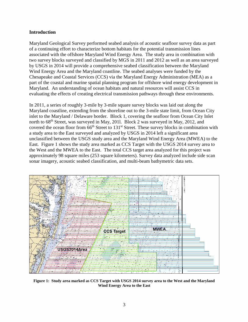
In 2011, a series of roughly 3-mile by 3-mile square survey blocks was laid out along the

Maryland coastline, extending from the shoreline out to the 3-mile state limit, from Ocean City

inlet to the Maryland / Delaware border. Block 1, covering the seafloor from Ocean City Inlet

north to 68th Street, was surveyed in May, 201l. Block 2 was surveyed in May, 2012, and

covered the ocean floor from 66th Street to 131st Street. These survey blocks in combination with

a study area to the East surveyed and analyzed by USGS in 2014 left a significant area

unclassified between the USGS study area and the Maryland Wind Energy Area (MWEA) to the

East. Figure 1 shows the study area marked as CCS Target with the USGS 2014 survey area to

the West and the MWEA to the East. The total CCS target area analyzed for this project was

approximately 98 square miles (253 square kilometers). Survey data analyzed include side scan

sonar imagery, acoustic seabed classification, and multi-beam bathymetric data sets.

Figure 1: Study area marked as CCS Target with USGS 2014 survey area to the West and the Maryland

Wind Energy Area to the East

4

Field Methodology

Survey Parameters

The field surveys were conducted for NOAA by SAIC on board M/V Atlantic Surveyor. Full

reports and associated files are available for download at https://data.noaa.gov/dataset. Sheet

H11649 was surveyed from August 17, 2007 to November 18, 2007. Sheet H11650 was

surveyed from September 29, 2007 to November 18, 2007. Sheet H11872 was surveyed from

July 16, 2008 to December 19, 2008. Sheet H11873 was surveyed from October 13, 2008 to

December 18, 2008.

Positional data was supplied using the M/V Atlantic Surveyor’s onboard GPS and depth

sounding system. Horizontal coordinates were collected using a Trimble 4000 survey-grade

GPS receiver with Trimble Probeacon Differential Global Positioning System (DGPS). The

vessel altitude was acquired using TSS POS/MV Inertial Navigation System using TSS POS/MV

320.

Bathymetric Echosounder

Raw bathymetric data were collected using a RESON SeaBat 8101 ER multibeam sonar system.

DGPS differential corrections broadcast by the United States Coast Guard (USCG) in

combination with GPS satellite data provide a horizontal accuracy of 1 meter. The data was

processed using an 81P sonar processor. Speed of sound corrections were provided using

Brooke Ocean Technology, Ltd, Moving Vessel Profiler-30 in conjunction with a Sea-Bird

Electronics, Inc. SBE 19 CTD Profiler

Side Scan Sonar

A Klein 3000 side scan sonar system was used to image the seafloor. The underwater sensor

(fish) was adjusted to depth throughout the survey. Side scan data was logged in eXtended

Triton Format (XTF) and maintained at full resolution.

Analytical Methods

Bathymetry

All depth data presented in this study were referenced to MLLW at the Ocean City Fishing Pier.

All processing and corrections were completed prior to MGS acquisition of the dataset from

NOAA. No post corrections were required.

Side scan sonar mosaic

Side scan sonar data were processed using Chesapeake Technology’s SonarWiz 5 software. This

software generates georeferenced side scan sonar mosaics and track line geometry. The mosaics

5

(.tif format) represent an image of the seafloor, based on surface sediment acoustic reflectivity.

The side scan data sets for all sheets were combined into a single SonarWiz project to produce a

compiled mosaic image. The .tif mosaic raster image was classified using ESRI ArcGIS using

the maximum likelihood classification processor. Images (.bmp format) of the seafloor along

each individual trackline are also produced, but are not georeferenced. These “waterfall” images

are free of the typical distortions introduced by georeferencing, and are the highest resolution

seafloor imagery available from this software.

GIS Products

GIS data were compiled with ESRI ArcGIS Desktop 10.2.2. All GIS coordinate data were

projected to UTM 18N (WGS 1984). Final map products and data layers are available in various

ArcGIS and graphic formats.

6

Results

The study area covered portions of four NOAA survey sheets. The area covered was 98 square

miles (253 km2). The study area in relation to the NOAA survey sheets is shown in Figure 2.

Figure 2: Study area in relation to NOAA Sheet survey blocks

7

Bathymetry

Figure 3 shows a bathymetric map of the survey area. Data were derived from published NOAA

datasets available from the NOAA Geophysical Data Center. Bathymetry was collected between

2007 and 2008 using a Reson SeaBat 8101 multibeam echosounder. Data were corrected to

mean lower low water and projected in UTM 18N (meters) NAD83. This data set was used to

create a hillshade bathymetric map as well as 1 meter contours (Figures 3 and 4).

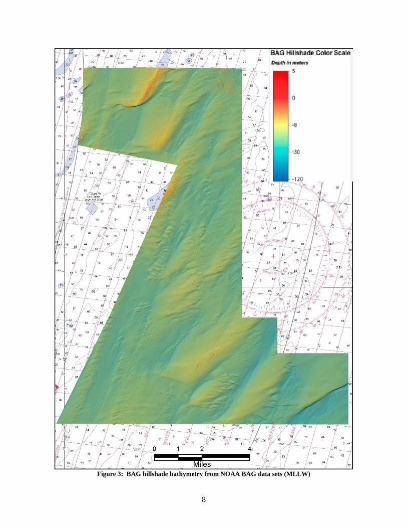
8

Figure 3: BAG hillshade bathymetry from NOAA BAG data sets (MLLW)

9

Figure 4: -1 meter bathymetric contours from NOAA BAG data sets (MLLW) overlying the

hillshade

10

Side Scan Sonar

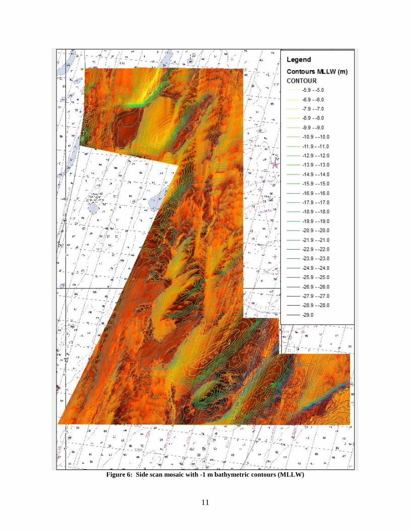
The side scan sonar mosaic is presented in Figure 5. In this rendering darker areas are low-

backscatter/fine sediments and lighter areas are higher-backscatter/coarser sediments. Figure 6

shows this mosaic with -1 meter contours to demonstrate the relationship between depth and

bottom features.

Figure 5: Study area side scan mosaic

11

Figure 6: Side scan mosaic with -1 m bathymetric contours (MLLW)

12

Acoustic Seabed Classes

Bottom sediment composition is influenced by bottom geomorphology, water depth, substrate

composition and biologic activity. The interaction of these factors with water column energy,

such as waves and currents, determines in part the seafloor surface composition. Sediments

often range from mud and muddy sand to coarse sand and gravel over an area of a few meters.

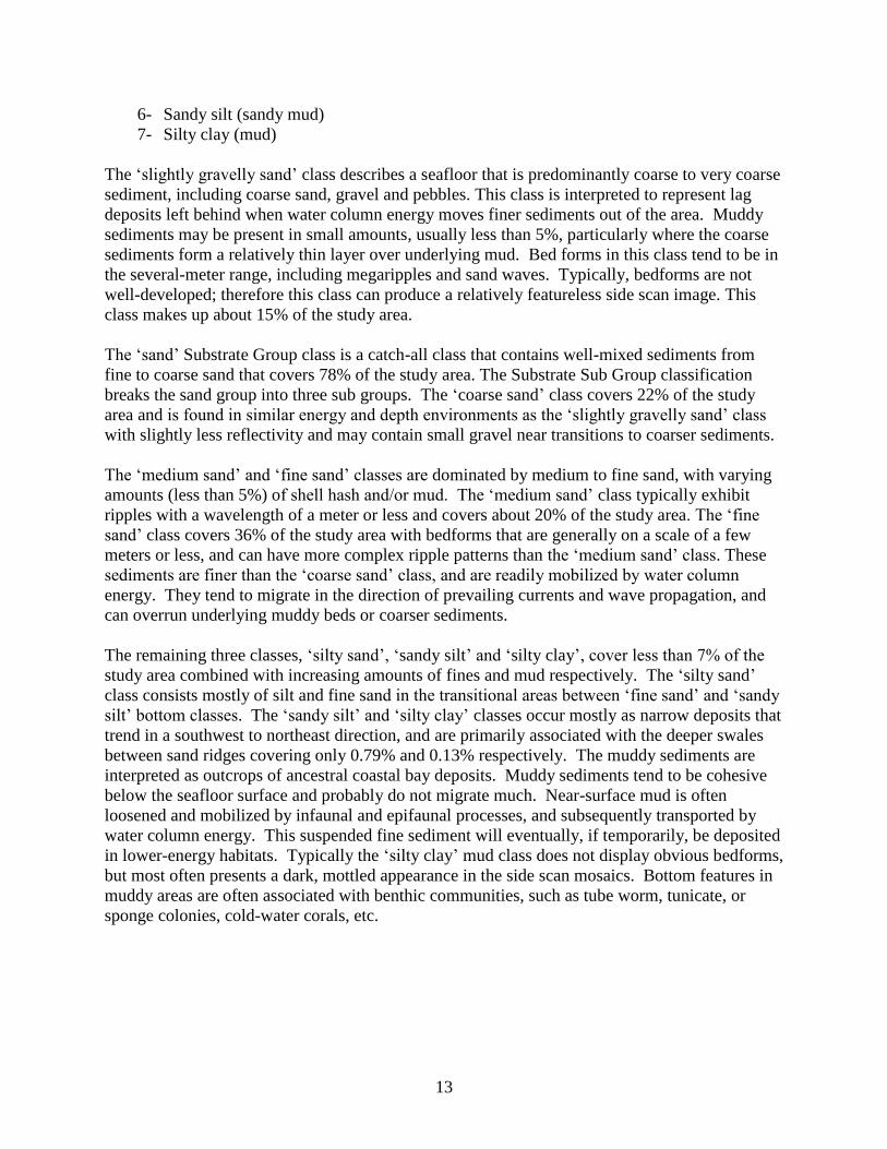
The compiled side scan sonar mosaic raster was classified using Image Classification in ArcGIS

Spatial Analyst. The classification software extracts information classes from the multiband

mosaic raster image to produce a raster image that represents bottom classes with graded colors.

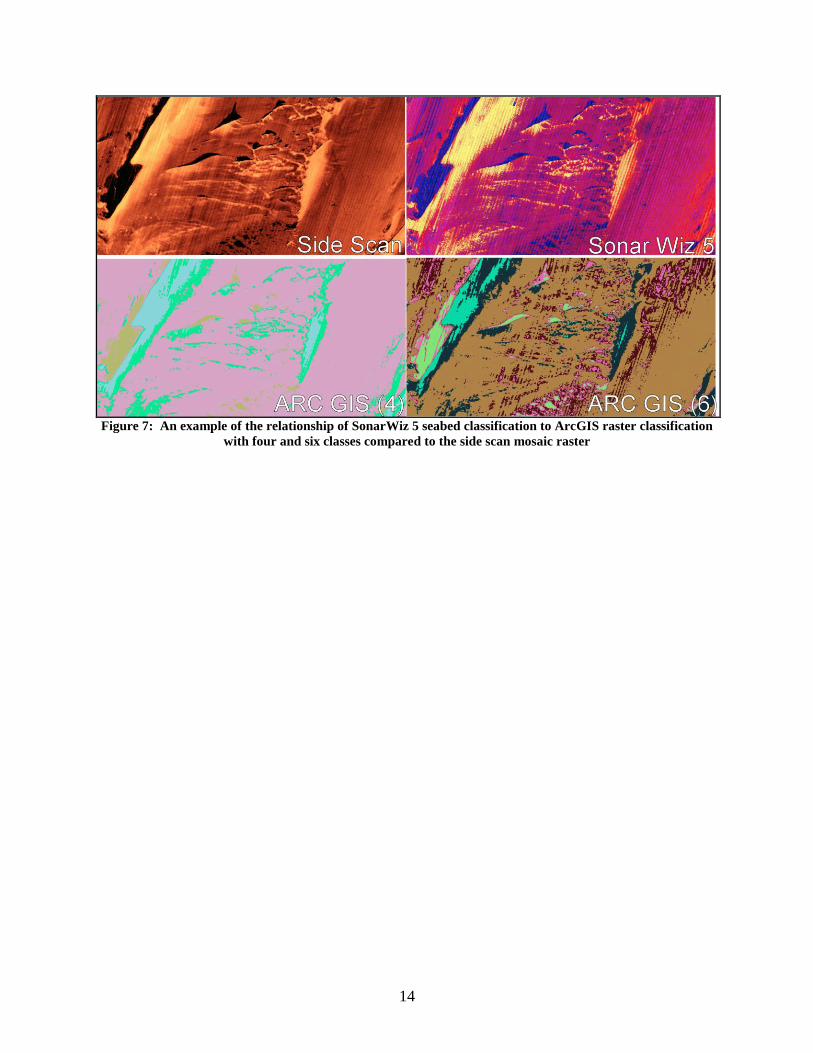
Two supervised classifications were performed to create rasters with four and six classes based

on the training samples signature files and are shown in Figures 8 and 9 respectively. A similar

process can also be performed using SonarWiz 5 with the exception that SonarWiz analyzes each

sonar line file individually. The data set for this project was too large for SonarWiz processing.

A comparison of the side scan mosaic, Sonar Wiz 5 classification, and the ArcGIS classifications

are shown in Figure 7. The classification analysis of the side scan raster data indicated that a

combination of the four and six class classification rasters be used. This resulted in an optimum

number of acoustically distinct bottom types in this area of seven. By grouping some similar

classes that were in both the four and six class rasters together, eliminating signal noise, and

integrating small, distinct classes into surrounding larger classes, the seven major bottom types

emerged. These types were correlated with bottom grab samples and bathymetry to produce a

map of bottom classes, based on dominant sediment types. Table 1 lists grab sample

characteristics and sample locations are shown in Figure 10.

By comparing the acoustic raster analysis with bottom samples, side scan imagery and

bathymetry, patterns of sediment types become evident. The seafloor bottom types were

digitized in ArcGIS to indicate the areas of distinct bottom classes. Each class was then classified

based on the Federal Geographic Data Committee (FGDC) Coastal and Marine Ecological

Classification Standard (CMECS) substrate classification for unconsolidated mineral substrate.

Figure 11 shows the bottom class map for the five Substrate Group classes derived from these

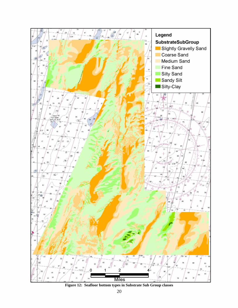
various data sources. The bottom class map for the Substrate Sub Group breaks the sand bottom

class in the Substrate Group further into coarse, medium and fine sand classes. The resulting

Substrate Sub Group bottom class map contains seven bottom classes and is shown in Figure 12.

These classes are necessarily broad due to the highly variable surface sediment composition.

The classification process attempts to select the dominant acoustic class in a given area, which

may contain several acoustic classes. The square kilometer area of each class as well as the

percent of the survey area covered is shown in Table 2. In the surveyed region, surface sediments

in the Substrate Sub Class tend to group into seven classes. The Substrate Group is listed in

parenthesis.

1- Slightly gravelly sand (slightly gravelly)

2- Coarse sand (sand)

3- Medium sand (sand)

4- Fine sand (sand)

5- Silty sand (muddy sand)

13

6- Sandy silt (sandy mud)

7- Silty clay (mud)

The ‘slightly gravelly sand’ class describes a seafloor that is predominantly coarse to very coarse

sediment, including coarse sand, gravel and pebbles. This class is interpreted to represent lag

deposits left behind when water column energy moves finer sediments out of the area. Muddy

sediments may be present in small amounts, usually less than 5%, particularly where the coarse

sediments form a relatively thin layer over underlying mud. Bed forms in this class tend to be in

the several-meter range, including megaripples and sand waves. Typically, bedforms are not

well-developed; therefore this class can produce a relatively featureless side scan image. This

class makes up about 15% of the study area.

The ‘sand’ Substrate Group class is a catch-all class that contains well-mixed sediments from

fine to coarse sand that covers 78% of the study area. The Substrate Sub Group classification

breaks the sand group into three sub groups. The ‘coarse sand’ class covers 22% of the study

area and is found in similar energy and depth environments as the ‘slightly gravelly sand’ class

with slightly less reflectivity and may contain small gravel near transitions to coarser sediments.

The ‘medium sand’ and ‘fine sand’ classes are dominated by medium to fine sand, with varying

amounts (less than 5%) of shell hash and/or mud. The ‘medium sand’ class typically exhibit

ripples with a wavelength of a meter or less and covers about 20% of the study area. The ‘fine

sand’ class covers 36% of the study area with bedforms that are generally on a scale of a few

meters or less, and can have more complex ripple patterns than the ‘medium sand’ class. These

sediments are finer than the ‘coarse sand’ class, and are readily mobilized by water column

energy. They tend to migrate in the direction of prevailing currents and wave propagation, and

can overrun underlying muddy beds or coarser sediments.

The remaining three classes, ‘silty sand’, ‘sandy silt’ and ‘silty clay’, cover less than 7% of the

study area combined with increasing amounts of fines and mud respectively. The ‘silty sand’

class consists mostly of silt and fine sand in the transitional areas between ‘fine sand’ and ‘sandy

silt’ bottom classes. The ‘sandy silt’ and ‘silty clay’ classes occur mostly as narrow deposits that

trend in a southwest to northeast direction, and are primarily associated with the deeper swales

between sand ridges covering only 0.79% and 0.13% respectively. The muddy sediments are

interpreted as outcrops of ancestral coastal bay deposits. Muddy sediments tend to be cohesive

below the seafloor surface and probably do not migrate much. Near-surface mud is often

loosened and mobilized by infaunal and epifaunal processes, and subsequently transported by

water column energy. This suspended fine sediment will eventually, if temporarily, be deposited

in lower-energy habitats. Typically the ‘silty clay’ mud class does not display obvious bedforms,

but most often presents a dark, mottled appearance in the side scan mosaics. Bottom features in

muddy areas are often associated with benthic communities, such as tube worm, tunicate, or

sponge colonies, cold-water corals, etc.

14

Figure 7: An example of the relationship of SonarWiz 5 seabed classification to ArcGIS raster classification

with four and six classes compared to the side scan mosaic raster

15

Figure 8: ArcGIS maximum likelihood classification of the side scan mosaic for six classes

16

Figure 9: ArcGIS maximum likelihood classification of the side scan mosaic for four classes

17

Table 1: Bottom sampling locations and grab sample descriptions

Block ID Sample

NAD83 Latitude Longitude

UTM NAD83 (m) Northing Easting

Bottom Type

Depth (m)

Charted Bottom

11649 BS-16 38.429361 74.98075 4253455.45 501680.20 med S Sh 14.18 S Sh

11649 BS-10 38.459556 74.975806 4256805.94 502110.88 fne S Sh 17.15 S Sh

11650 BS-4 38.460111 74.908861 4256871.24 507951.50 med S 14.07 S Sh

11650 BS-5 38.458361 74.870472 4256681.07 511301.05 med S Sh 19.33 S Sh

11650 BS-8 38.451861 74.877667 4255958.97 510674.30 med S fne G 17.67 h

11650 BS-9 38.436444 74.929972 4254243.56 506111.64 crs S med G 13.74 S Sh

11650 BS-10 38.427417 74.871944 4253247.28 511177.37 fne S 15.28 S Sh

11650 BS-12 38.374556 74.924083 4247376.79 506631.24 fne S 13.87 S

11650 BS-13 38.3435 74.920361 4243931.18 506959.34 crs S fne G 17.26 S Sh

11650 BS-14 38.344222 74.890278 4244014.01 509588.12 fne S 15.79 S Sh

11872 G_BS-7 38.342722 74.890639 4243847.53 509556.76 medS brkSh 14.67 S Sh

11872 G_BS-8 38.317833 74.925 4241082.91 506556.28 medS brkSh 16.12 c S

11872 G_BS-16 38.259778 74.962889 4234639.19 503246.73 medS brkSh 17.67 f S

Table 2: Area of seafloor bottom types and percent of study site covered for CMECS Substrate

Group and Substrate SubGroup

Substrate Group Area (sq. km) Percent Substrate SubGroup Area (sq. km) Percent

Slightly Gravelly 37.48 14.80

Slightly Gravelly Sand 37.48 14.80

Sand 198.23 78.29

Coarse Sand 55.30 21.84

Muddy Sand 15.16 5.99

Medium Sand 51.71 20.42

Sandy Mud 2.01 0.79

Fine Sand 91.22 36.03

Mud 0.32 0.13

Silty Sand 15.16 5.99

Sandy Silt 2.01 0.79

Silty Clay 0.32 0.13

18

Figure 10: Grab sample locations

19

Figure 11: Seafloor bottom types in Substrate Groups classes

20

Figure 12: Seafloor bottom types in Substrate Sub Group classes

21

Figure 13. Seafloor Sub Group bottom types with -1m contours overlaid

22

Summary

The study area seafloor adjacent to the Maryland Wind Energy Area is highly dynamic,

displaying a variety of surface features and sediment types. The study area is dominated by

sands with 15% gravelly sand, 78% fine to coarse sand, and 7% silty sand to clayey mud. The

sands fine to coarse sands were separated into fine, medium and coarse which coverage of 36%,

20% and 22% respectively. Of the 7% classified as silty sand to clayey mud, only 1% of the

study area contains silty mud and clayey mud. The most mobile sediment classes appear to be

the fine and medium sand and non-cohesive mud, (which is not a formal class). Fine- to

medium- sand bodies exhibit several bedforms, and form sheet and ribbon deposits on the

seafloor surface. These deposits can migrate over relatively short periods, from days to weeks,

depending on available water column energy. Non-cohesive mud is highly mobile, suspended by

relatively little water column energy and deposited in low energy environments. This mobile,

very fine sediment is probably derived from cohesive mud outcrops that are reworked by

infaunal and epifaunal activity, which exposes the mud to wave and current motion. It forms

ephemeral surface deposits in the troughs of bedforms and other low areas, tends to be aerially

limited to less than a few square meters, and is readily resuspended.

The least mobile classes are coarse sand, slightly gravelly sand and cohesive clayey mud.

Coarse sediments tend to form lag deposits because they require more energy to mobilize than is

ordinarily present in the regional water column. Only during extreme conditions is there enough

current or wave energy to move coarse material. These coarser sediments were found

predominantly on the crests of shoals. The cohesive clayey mud, mostly found in bottom

outcrops in deeper water, resists mobilization due its cohesiveness.

Generally, the clayey silt to fine sand classes are associated with deeper water and swales

between ridges. The sand Substrate Group class, which is highly mixed and heterogeneous, can

occur at all depths, since it is formed in mixed-energy environments and as a transitional class

between coarse and fine sediment-dominated areas. The coarse sand and slightly gravely sand

classes are found in elevated areas, slopes and channels where there is sufficient energy to

winnow fine and medium sand, leaving the coarser fraction in place.

23

References 1 Coastal and Marine Ecological Classification Standard. Federal Geographic Data Committee

(2012): 276. July 2012. Web

Appendices

I. GIS data supplement to this report

24

Appendix I: GIS data supplement to this report

A DVD containing GIS data sets and images accompanies, or is available for, this report. The

following items are included.

ArcGIS 10.2.2 file geodatabase:

OffshoreWindHabitats.gdb

o

ArcGIS 10.2.2 map file for use with geodatabase:

OffshoreWindHabitats.mxd

ArcGIS 10.2.2 shape files derived from geodatabase:

Contours1mMLLW

NOAA_Samples

Side scan sonar mosaics:

SideScan_OffshoreWindCompiled.tif: 1-meter resolution, UTM 18N (WGS84)

Ground-truth data:

NOAA_Samples_Target.shp: Sample locations and descriptions

Seabed classification rasters:

Arc Classification 4 Classes.tif: ArcGIS 10.2.2 raster classification, 4 bottom classes,

TIF format

Arc Classification 6 Classes.tif: ArcGIS 10.2.2 raster classification, 6 bottom classes,

TIF format

Layers:

ArcGIS 10.2.2 layer files for geodatabase display

Navigation chart:

NOAA Navigation chart 12211_1, Cape Henlopen to Fenwick Island