Dear Editor, Thank you for giving us the opportunity to revise this manuscript. The author appreciates thetime and details provided by the editor and the reviewers. The insightful suggestions havecertainly improved the manuscript. Below, you will find detailed response to reviewers’comments.

Reviewer A: Changes which must be made before publication: This paper presents a virtual class of non-conforming finite element method. The method has been analyzed and the analysis seems to be rigorous. Thus, the paper can be accepted with some revision.

1. Please explain the virtual class in more detail and what is main advantage?• Agreed and added in Introduction section ; Virtual finite element is a finite elementinspired by the classical Crouzeix-Raviart which does not require the computingvalues of basis functions at the midpoint of edges and faces. It maintains also thecapability to reproduce several physical models exactly in 2D/3D, and to treat theheterogeneous domains with discontinuity such as the Stokes interface problems.Moreover, it is really simple to implement and avoids the locking-free during meshrefinement for shells and this is why I think it is a really good one.

2. The literature review is a bit weak. Please extend the literature review a bit to includethe latest studies (if any).

• Agreed and added, See References ( references begin at to ).

3. The conclusions can be extended slightly to discuss the possible limitations and ways to improve this method in future work.

• Agreed and added. See Conclusion section.

4. Check all the mathematical formulas carefully. For example, Eq. (2.13) is incomplete with an "=".

• Agreed and corrected. See the equaton (2.13) in the text.

Reviewer B: Suggestions which would improve the quality of the paper but are not essential for publication: The main idea of the paper, is to propose a new class of nonconformingfinite element inspired by the classical Crouzeix-Raviart. The originality is to consider the degrees of freedom as the vertices of the simplex used for Crouzeix-Ravairt element. The authors give an optimal a priori error estimate. The numerical experiments confirm the theoretical results. The construction is correct and the manuscript is well written and deserves to be added in the literature. The subject and the results obtained are quite interesting. Then I recommend the publication of this article in the International Journal of Mathematical Modelling and Numerical Optimisation Changes which must be made before publication:I propose a few remarks that I’d ask to include as a minor revision :

1. Page 2 and 3. In the figures 1 and 2. The letter T is very small.• Agreed and corrected.

2. Page 3. In the equation (2.5), It seems to me that is missing - instead of +.• Agreed and corrected. See the equaton (2.5) in the text.

3. Page 5. The equation (2.13) is incomplete.• Agreed and corrected. See the equation (2.13) in the text.

4. Page 9. In the equation (4.2), it’s better to remove d^2 and consider it in the constant c. Same remarque for the equations (4.10), (4.11)

• Agreed and corrected.

5. Page 16. The bibliography must be harmonized, especially the way of the citing the journal. Take the initials of the journal names everywhere, instead of of taking the full name.

• Agreed and corrected. See References.

A virtual class of nonconforming finite elements and itsapplications to Poisson’s equation

Hammou El-Otmanya,˚

aEngineering Sciences Laboratory, Polydisciplinary Faculty of Taza, Sidi Mohamed

Ben-Abdellah University Fez, Morocco

Abstract

In this paper, we develop and analyze the virtual class of nonconformingFinite Element inspired from the classical Crouzeix-Raviart element in two andthree-dimensions. We focus on Poisson’s equation for theoretical and numericalresults. We show that the discrete problem is stable and the a priori errorestimates are optimal. Two numerical tests are presented to demonstrate thetheoretical results.

Keywords: Virtual finite element, Crouzeix-Raviart element, interpolationerror, consistency error, a priori error estimates.

1. Introduction

The nonconforming finite element methods are very popular method forthe numerical approximation of partial di↵erential equations, for they enjoybetter stability properties and smaller support compared to the conforming finiteelement methods. Moreover, it is easier to prove the inf-sup condition for Stokesequations and it is also quite simple to implement. One of the most popularnon-conforming finite element methods is the method based on discretizing withthe lowest order Crouzeix-Raviart element ([5], see [8] for many improvementsand generalizations). It is also known as simplicial P 1 nonconforming finiteelement which expression is piecewise linear polynomials with respect to thetriangulation of domain while degrees of freedom are the mean of the functionover the edges/facets (2D{3D). They interested many mathematicians andnumericians with di↵erent applications, see for example [1, 3, 4, 6, 10, 12, 17, 19].

Our interest in the topic of this work arose from the fact that there existoriginal papers which use and discuss the development of the nonconformingvirtual element method on polygonal and polyhedral meshes, see for instance, [7,11, 13–15, 18] and its applications to elliptic problem [19], to Stokes problem [21,23] and to elasticity problems [22, 25, 26]. Later Zhang et al in [26], developed

˚Corresponding authorEmail address: hamou.elotmany@gmail.com (Hammou El-Otmany)

Preprint submitted to International Journal of Mathematical Modelling and Numerical OptimisationMay 21, 2021

a nonconforming virtual element method on polygonal and polyhedral meshesand applied it to Navier-Stokes problem. The authors established the stabilityof discrete scheme, and that the convergence rates of error estimates in L

2andenergy norms are optimal.

Among the literature mentioned in the above, their virtual methods arebased on nonconforming finite elements on polygonal and polyhedral meshes.At my knowledge, none of them has proposed a new finite element with thedegrees of freedom are the vertices of the simplex used for a Crouzeix-Ravairtelement. Therefore, the main of this paper is to carry out the development andthe numerical analysis of a new class of nonconforming finite element inspiredby the classical Crouzeix-Raviart. Indeed, this element does not require thecomputing values of basis functions at the midpoint of edges and faces. Itmaintains also the capability to reproduce several physical models exactly in2D/3D, and to treat the heterogeneous domains with discontinuity such as theStokes interface problems. Moreover, it is really simple to implement and avoidsthe locking-free during mesh refinement for shells and this is why I think it is areally good one.

The rest of this paper is organized as follows: First, we introduce and de-velop the virtual family of Crouzeix-Raviart finite element. Then, in the thirdsection, we introduce the useful notations, Poisson’s equation and its associatedweak formulation by considering the new triangular/tetrahedral nonconformingfinite element. In the fourth, we establish the estimate of interpolation error forour finite element. Then, in the fifth section, we interest in consistency errorand we establish the results proving the optimal convergence of a priori error es-timates. In the final section of this paper we present two numerical experimentsto demonstrate the theoretical results and we draw the conclusion.

Throughout the paper we consider the following convention concerning abound constant. We will note by c a positive constant independent of theindices and the simplex. Thus, we do not need to precise its expression and itmay vary from one line to the other, and even in the same line.

2. Virtual class of nonconforming finite element

Let T be non-degenerate simplex in Rd, d “ 2, 3 that composed of a�ned-simplices (i.e. triangles if d “ 2 or tetrahedrons if d “ 3) with vertices vi, i Pt1, ¨ ¨ ¨ , d`1u and d-dimensional Lebesgue measure |T |. By �i, i P t1, ¨ ¨ ¨ , d`1u,we denote the barycentric coordinates for a point vi, i P t1, ¨ ¨ ¨ , d ` 1u, relativeto a simplex T . Moreover, we introduce Fi, i P t1, ¨ ¨ ¨ , d ` 1u the facets of Tsuch that Fi means an edge in R2 and face in R3, but this distinction will notbe made unless necessary. Finally, we introduce the simplex T which containsT with vertices vi, i P t1, ¨ ¨ ¨ , d`1u. To ease the notation, we occasionally referto T Ä Rd and T Ä Rd, see Figure 1.

To develop our finite element, we first introduce briefly the d-dimensionalCrouzeix-Raviart element on T ;

`T, P

1pT q,⌃CR˘and it is expressed by:

1. P1pT q is the space of polynomials of degree 1 on T .

2

2. The degrees of freedom of Crouzeix-Raviart are

⌃CRT :“ t�CR

i , i “ 1, 2, ¨ ¨ ¨ , d ` 1u (2.1)

with

�CRi :“ 1

measpFiq

ª

Fi

vds, i “ 1, 2, ¨ ¨ ¨ , d ` 1. (2.2)

In addition, the basis functions in terms of the barycentric coordinates ofthe edge/face, see [9], are expressed in the form:

'CRi pxq “ d

ˆ1

d´ �ipxq

˙, i “ 1, 2, ¨ ¨ ¨ , d ` 1. (2.3)

In this work, we interest in development of a new finite element in the simplexT (see Figures 1 and 2). To do this, we introduce the notation of vertices vi onT such that

vi “d`1ÿ

j“1,j‰i

vj ` p1 ´ dqvi (2.4)

Hence, (2.4) can be rewritten as follows:

vi “d`1ÿ

j“1

vj ´ dvi (2.5)

By using the above notations, we cite the following lemma which is the keyto development of our finite element.

Lemma 2.1. Let T be a simplex with vertices vi, i “ 1, ¨ ¨ ¨ , d ` 1. Then T is

non-degenerate with vertices vi, i “ 1, ¨ ¨ ¨ , d ` 1

Proof. By using (2.5), we have

vi ´ v1 “d`1ÿ

j“1

vj ` dvi ´˜

d`1ÿ

j“1

vj ` dv1

¸“ ´dvi ` dv1

“ ´dpvi ´ v1q

Thus, by multiplying both sides of the last equation by ↵i and summing fori “ 2 to pd ` 1q, we obtain

d`1ÿ

i“2

↵ipvi ´ v1q “ ´d

d`1ÿ

i“2

↵ipvi ´ v1q (2.6)

Finally, from the above equation (2.6), we have

↵i “ 0, i “ 2, ¨ ¨ ¨ , d ` 1. (2.7)

Here, we use that the simplex T is non-degenerate, then the elements of tvi ´v1, i “ 2, ¨ ¨ ¨ , d ` 1u are linearly independent.

3

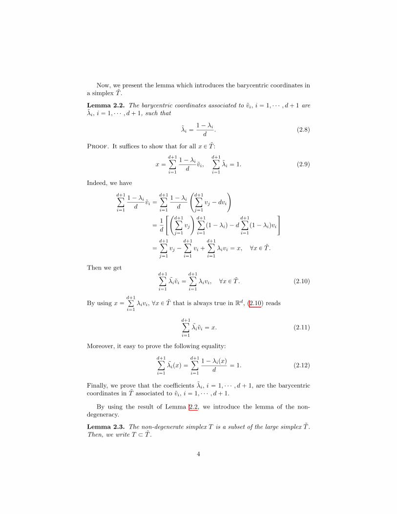
Now, we present the lemma which introduces the barycentric coordinates ina simplex T .

Lemma 2.2. The barycentric coordinates associated to vi, i “ 1, ¨ ¨ ¨ , d ` 1 are

�i, i “ 1, ¨ ¨ ¨ , d ` 1, such that

�i “ 1 ´ �i

d. (2.8)

Proof. It su�ces to show that for all x P T :

x “d`1ÿ

i“1

1 ´ �i

dvi,

d`1ÿ

i“1

�i “ 1. (2.9)

Indeed, we have

d`1ÿ

i“1

1 ´ �i

dvi “

d`1ÿ

i“1

1 ´ �i

d

˜d`1ÿ

j“1

vj ´ dvi

¸

“ 1

d

«˜d`1ÿ

j“1

vj

¸d`1ÿ

i“1

p1 ´ �iq ´ d

d`1ÿ

i“1

p1 ´ �iqvi�

“d`1ÿ

j“1

vj ´d`1ÿ

i“1

vi `d`1ÿ

i“1

�ivi “ x, @x P T .

Then we getd`1ÿ

i“1

�ivi “d`1ÿ

i“1

�ivi, @x P T . (2.10)

By using x “d`1∞i“1

�ivi, @x P T that is always true in Rd, (2.10) reads

d`1ÿ

i“1

�ivi “ x. (2.11)

Moreover, it easy to prove the following equality:

d`1ÿ

i“1

�ipxq “d`1ÿ

i“1

1 ´ �ipxqd

“ 1. (2.12)

Finally, we prove that the coe�cients �i, i “ 1, ¨ ¨ ¨ , d ` 1, are the barycentriccoordinates in T associated to vi, i “ 1, ¨ ¨ ¨ , d ` 1.

By using the result of Lemma 2.2, we introduce the lemma of the non-degeneracy.

Lemma 2.3. The non-degenerate simplex T is a subset of the large simplex T .

Then, we write T Ä T .

4

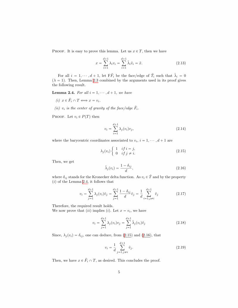
Proof. It is easy to prove this lemma. Let us x P T , then we have

x “d`1ÿ

i“1

�ivi “d`1ÿ

i“1

�ivi “ x. (2.13)

For all i “ 1, ¨ ¨ ¨ , d ` 1, let FFi be the face/edge of Ti such that �i “ 0(� “ 1). Then, Lemma 2.3 combined by the arguments used in its proof givesthe following result.

Lemma 2.4. For all i “ 1, ¨ ¨ ¨ , d ` 1, we have

(i) x P Fi X T ñ x “ vi.

(ii) vi is the center of gravity of the face/edge Fi.

Proof. Let vi P P pT q then

vi “d`1ÿ

i“1

�jpviqvj , (2.14)

where the barycentric coordinates associated to vi, i “ 1, ¨ ¨ ¨ , d ` 1 are

�jpviq"

1 if i “ j,

0 if j ‰ i.(2.15)

Then, we get

�jpviq “ 1 ´ �ij

d, (2.16)

where �ij stands for the Kronecker delta function. As vi P T and by the property(i) of the Lemma 2.4, it follows that

vi “d`1ÿ

j“1

�jpviqvj “d`1ÿ

j“1

1 ´ �ij

dvj “ 1

d

d`1ÿ

i“1,j‰i

vj (2.17)

Therefore, the required result holds.We now prove that (ii) implies (i). Let x “ vi, we have

vi “d`1ÿ

j“1

�jpviqvj “d`1ÿ

j“1

�jpviqvj (2.18)

Since, �jpviq “ �ij , one can deduce, from (2.15) and (2.16), that

vi “ 1

d

d`1ÿ

j“1,j‰i

vj . (2.19)

Then, we have x P Fi X T , as desired. This concludes the proof.

5

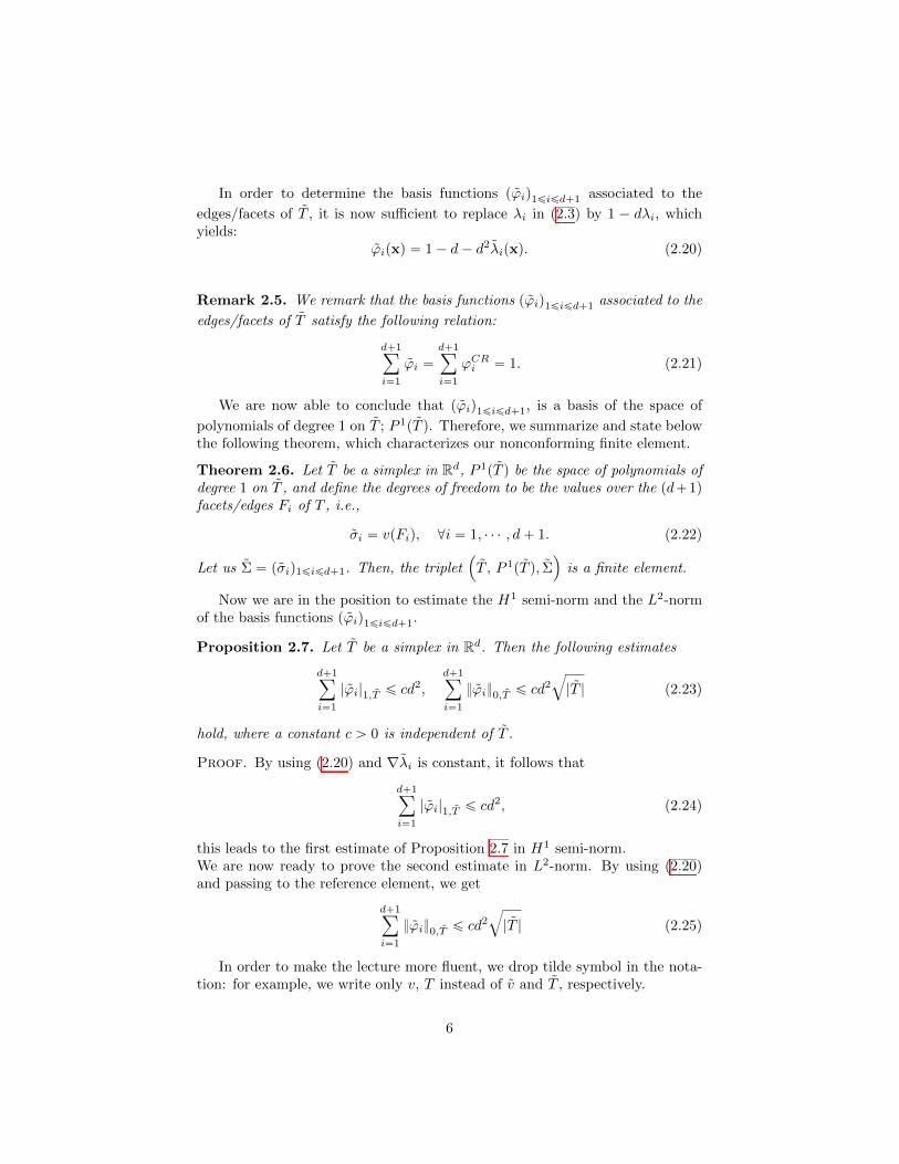
In order to determine the basis functions p'iq1§i§d`1 associated to the

edges/facets of T , it is now su�cient to replace �i in (2.3) by 1 ´ d�i, whichyields:

'ipxq “ 1 ´ d ´ d2�ipxq. (2.20)

Remark 2.5. We remark that the basis functions p'iq1§i§d`1 associated to the

edges/facets of T satisfy the following relation:

d`1ÿ

i“1

'i “d`1ÿ

i“1

'CRi “ 1. (2.21)

We are now able to conclude that p'iq1§i§d`1, is a basis of the space of

polynomials of degree 1 on T ; P 1pT q. Therefore, we summarize and state belowthe following theorem, which characterizes our nonconforming finite element.

Theorem 2.6. Let T be a simplex in Rd, P

1pT q be the space of polynomials of

degree 1 on T , and define the degrees of freedom to be the values over the pd`1qfacets/edges Fi of T , i.e.,

�i “ vpFiq, @i “ 1, ¨ ¨ ¨ , d ` 1. (2.22)

Let us ⌃ “ p�iq1§i§d`1. Then, the triplet

´T , P

1pT q, ⌃¯is a finite element.

Now we are in the position to estimate the H1 semi-norm and the L

2-normof the basis functions p'iq1§i§d`1.

Proposition 2.7. Let T be a simplex in Rd. Then the following estimates

d`1ÿ

i“1

|'i|1,T § cd2,

d`1ÿ

i“1

}'i}0,T § cd2b

|T | (2.23)

hold, where a constant c ° 0 is independent of T .

Proof. By using (2.20) and r�i is constant, it follows that

d`1ÿ

i“1

|'i|1,T § cd2, (2.24)

this leads to the first estimate of Proposition 2.7 in H1 semi-norm.

We are now ready to prove the second estimate in L2-norm. By using (2.20)

and passing to the reference element, we get

d`1ÿ

i“1

}'i}0,T § cd2b

|T | (2.25)

In order to make the lecture more fluent, we drop tilde symbol in the nota-tion: for example, we write only v, T instead of v and T , respectively.

6

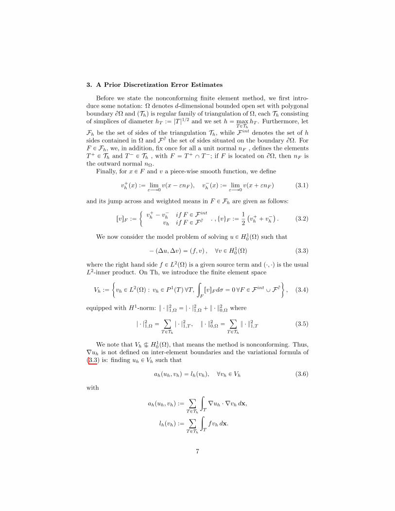
3. A Prior Discretization Error Estimates

Before we state the nonconforming finite element method, we first intro-duce some notation: ⌦ denotes d-dimensional bounded open set with polygonalboundary B⌦ and pThq is regular family of triangulation of ⌦, each Th consistingof simplices of diameter hT :“ |T |1{2 and we set h “ max

TPTh

hT . Furthermore, let

Fh be the set of sides of the triangulation Th, while Fint denotes the set of h

sides contained in ⌦ and FB the set of sides situated on the boundary B⌦. For

F P Fh, we, in addition, fix once for all a unit normal nF , defines the elementsT

` P Th and T´ P Th , with F “ T

` X T´; if F is located on B⌦, then nF is

the outward normal n⌦.Finally, for x P F and v a piece-wise smooth function, we define

v`h pxq :“ lim

"›Ñ0vpx ´ "nF q, v

´h pxq :“ lim

"݄0vpx ` "nF q (3.1)

and its jump across and weighted means in F P Fh are given as follows:

rvsF :“"

v`h ´ v

´h if F P F

int

vh if F P FB . , tvuF :“ 1

2

`v

`h ` v

´h

˘. (3.2)

We now consider the model problem of solving u P H10 p⌦q such that

´ p�u,�vq “ pf, vq , @v P H10 p⌦q (3.3)

where the right hand side f P L2p⌦q is a given source term and p¨, ¨q is the usual

L2-inner product. On Th, we introduce the finite element space

Vh :“"vh P L

2p⌦q : vh P P1pT q @T,

ª

FrvsF d� “ 0@F P F

int Y FB*, (3.4)

equipped with H1-norm: } ¨ }21,⌦ “ | ¨ |21,⌦ ` } ¨ }20,⌦ where

| ¨ |21,⌦ “ÿ

TPTh

| ¨ |21,T , } ¨ }20,⌦ “ÿ

TPTh

} ¨ }21,T (3.5)

We note that Vh Ü H10 p⌦q, that means the method is nonconforming. Thus,

ruh is not defined on inter-element boundaries and the variational formula of(3.3) is: finding uh P Vh such that

ahpuh, vhq “ lhpvhq, @vh P Vh (3.6)

with

ahpuh, vhq :“ÿ

TPTh

ª

Truh ¨ rvh dx,

lhpvhq :“ÿ

TPTh

ª

Tfvh dx.

7

The uniform Vh-stability of ahp¨, ¨q is completely standard. Then, it givesthe well-posedness in the variational formula (3.6). In addition, the a priori

error estimate satisfies the Strang Lemma [6]:

}u ´ uh}1,⌦ § c

ˆinf

vhPVh

}u ´ vh}1,⌦ ` supwhPVh,wh‰0

|ahpu ´ uh, whq|}wh}1,⌦

˙(3.7)

where the constant c is independent of h. In the sequel, we will be interestedin estimating of the interpolation error and the consistency error estimate of(3.7). The first one is estimated by using vh “ Ihv with the suitably definedinterpolation operator Ih, see the section 4 A second one is treated by theGalerkin orthogonality described in section 5.

4. Interpolation error estimates

In this section we establish the interpolation error estimates for both twoand three dimensions under considerations. For our finite element

`T, P

1pT q,�˘,

we denote by IT the local interpolation operator defined from HspT q to P

1pT qwith s “ 1, 2, by means of the previous degrees of freedom, associated to theedges/faces such that:

IT :“d`1ÿ

i“1

ˆ1

measpFiq

ª

Fi

v d�

˙'pxq, x P Rd (4.1)

where ', i “ 1, ¨ ¨ ¨ , d ` 1, are given by .Now, we are in the position to define the global interpolation operator Ih :

Hsp⌦q ›Ñ Vh by its restriction on any T P Th. In what follows, we will be

estimate the H1 semi-norm and L

2-norm on ⌦ of v ´ Ihv. To do this, we needthe following a priori error estimate of v ´ IT v on simplex T :

Lemma 4.1. Let T P Th. There exists a constant c ° 0 independent of h, such

that for all v P H2p⌦q:

|v ´ Ihv|1,T § c hT |v|2,T , }v ´ Ihv}0,T § c h2T |v|2,T . (4.2)

Proof. The proof is analogous to the one given in [9], and it is based on theBramble-Hilbert lemma (cf. [6]) and the passage to the reference simplex T ofcoordinates p0, 0q, p1, 0q and p0, 1q. As usually, let FT : T ›Ñ T be the a�netransformation with the corresponding Jacobian matrix JT , see [6]. Then, thefollowing inequalities

|v|m,T § c}JT }m|detpJT q|´1{2|v|m,T , @v P HmpT q, (4.3)

|v|m,T § c}J´1T }m|detpJT q|1{2|v|m,T , @v P H

mpT q (4.4)

hold, where

}J´1T } § hT

⇢T, }JT } § hT

⇢T

, |detpJT q| “ |T ||T |

.

8

We first interest in the interpolation error in H1 semi-norm on T “ F

´1T pT q.

We can write

|IT v|1,T §d`1ÿ

i“1

1

measpFiq

ˇˇª

Fi

vds

ˇˇ'i|1,T § c

˜d`1ÿ

i“1

|'i|1,T

¸}v}C0pT q. (4.5)

By using the Sobolev embedding theorem H2pT q Ä C

0pT q, we show that thereexists the constant c ° 0 independent of T such that:

|IT v|1,T § c

˜d`1ÿ

i“1

|'i|1,T

¸}v}2,T . (4.6)

We can now apply the Bramble-Hilbert lemma to Fpvq “ |v ´ IT v|1,T , we have:

|v ´ IT v|1,T § c

˜d`1ÿ

i“1

|'i|1,T

¸|v|2,T . (4.7)

where the constant c ° 0 is independent of T .By putting together (4.3), (4.4) and ˆIT v “ IT v, we can get:

|v ´ IT v|1,T § c|v ´ IT v|1,T § c

˜d`1ÿ

i“1

|'i|1,T¸hT |v|2,T . (4.8)

By injecting (2.23) of Proposition 2.7 in (4.8), we deduce existence of a constantc ° 0 such that for any T P Th the following estimate holds:

|v ´ IT v|1,T § cd2hT |v|2,T . (4.9)

In order to estimate the interpolation error in L2 norm, we apply the same

techniques and we use (2.23) from Proposition 2.7, which proves the announcedresult.

By summing each result of Lemma 2.4 over all simplex T P Th, we get theestimate of the global interpolation error as follows.

Theorem 4.2. (global interpolation error). There exists a constant c ° 0 in-

dependent of h, such that for all v P H2p⌦q:

|v ´ Ihv|1,⌦ § c h|v|2,⌦, (4.10)

}v ´ Ihv}0,⌦ § c h2|v|2,⌦. (4.11)

5. Consistency error estimates

In this section we interest in the consistency error estimate for both twoand three dimensions under considerations. To do this, we require the followinglemma of Galerkin Orthogonality.

9

Lemma 5.1. Let u P H2p⌦q be the exact solution of (3.3), and uh be the

approximate solution of the variational formula (3.6). Then, for all vh P Vh,

the following Galerkin Orthogonality holds.

ahpu ´ uh, vhq “ÿ

FPFh

ª

FBnurvhsF ds. (5.1)

Proof. The proof is based on the integration by parts on ⌦ and on the use ofrelation rxysF “ rxsF tyuF ` txuF rysF . Then, we obtain

ahpu, vhq “ lhpvhq `ÿ

FPFh

ª

FrBnuvhsF ds. (5.2)

By putting together rBnusF “ 0 and ahpuh, vhq “ lhpvhq, we conclude with thedesired result.

In the sense of (3.7), it is our aim to derive the consistency error estimateas follows.

Theorem 5.2. (Consistency error). Let u P H2p⌦q be the exact solution of

(3.3). Then the consistency error estimate

supwhPVh, wh‰0

ahpu ´ uh, whq}wh}1,⌦

§ c h|u|2,⌦ (5.3)

holds, with a constant c ° 0 independent of h.

Proof. Estimate (5.3) is easy to proof by using the same steps in [9] and it isbased on the Galerkin Orthogonality Lemma 5.1. One has for any wh P Vh that

ahpu ´ uh, whq “ÿ

FPFh

ª

FBnurwhsF ds. (5.4)

By putting together, the Cauchy-Schwartz, the trace inequalities and the Lemma2.4 for estimating the interpolation operator Ih, one has that:

ÿ

FPFh

ª

FBnurwhsF ds “

ÿ

FPFh

ª

FBn pu ´ Ihq rwhsF ds (5.5)

§˜

ÿ

FPFh

|F |´1}Bnpu ´ Ihuq}20,F¸1{2 ˜

ÿ

FPFh

|F |}rwhs}20,F¸1{2

(5.6)

§ c|u|2,⌦˜

ÿ

TPTh

h2T |wh|21,T

¸1{2

§ c h|u|2,⌦}wh}1,⌦, (5.7)

and the desired result follows readily.

10

We conclude from (3.7) that the a priori error estimate with respect to H1-

norm holds, with a constant c ° 0 independent of h. In addition, by gatheringthe above result and the Aubin-Nitsch duality trick (cf. [2]), the L2-norm ofa priori error holds, where a constant c is independent of h. So, we omit thedetails and we announce the following theorem:

Theorem 5.3. Let u P H2p⌦q be the exact solution of (3.3) and let uh P Vh

be the approximate solution of the variational formula (3.6). Then the a priori

error estimate

}u ´ uh}1,⌦ § c h|u|2,⌦. (5.8)

holds, where c ° 0 is independent of h.

If, in addition, ⌦ is convex and f P L2p⌦q, then we have

}u ´ uh}0,⌦ § c h2|u|2,⌦. (5.9)

6. Numerical experiments

To validate our proposed finite element method inspired by Crouzeix-Ravairtelement method, di↵erent numerical experiments are investigated in two andthree dimensions. Theoretical results for the Poisson’s equation obtained fromthe a priori error analysis with respect to H

1-norm and L2-norm, see Theorem

5.3, will be confirmed by several basic test cases by using the following Poissonmodel in 2D and 3D: " ´�u “ f inı,⌦,

u “ g on B⌦. (6.1)

6.1. Convergence study in 2D

To confirm the optimal order a priori error estimate stated in Theorem 5.3,we study the error convergence for the two-dimensional Poisson’s equation (6.1)in the unit square ⌦ “ p0; 1qˆp0; 1q of R2. We choose the right-hand side f andthe boundary condition g such that the exact solution u of (6.1) is given by:

upx, yq “ 12 ` 11`x2 ` y

2 ` xy˘

` 17x3 ` 20y3. (6.2)

For uniform mesh refinements, we present in Table 1 the computed errors, inH

1 and L2 norms with the convergence rate calculated from the errors on two

consecutive refined meshes, exactly with N and 4N triangles. From the pre-sented table, we numerically obtain the optimal convergence rates (see Theorem5.3) as follows:

}u ´ uh}1,⌦ “ O

´N

´1{2¯

“ O phq , }u ´ uh}0,⌦ “ O`N

´1˘

“ O`h2˘. (6.3)

In Figure 3, we represent these convergence orders in a log ´ log scale. InFigure 4 from a qualitative point of view, we obtain the exact solution is veryclose to the discrete one, computed on the finest mesh with N “ 2084 triangles.

11

6.2. Convergence study in 3D

In this subsection, we present our numerical results to support the theoreticalanalysis also in three dimensions. The Poisson’s equation (6.1), is consideredon the domain p0; 1q ˆ p0; 1q ˆ p´1; 1q, where the volume force f is defined as

fpx, y, zq “ 9⇡3 sinp⇡xq sinp⇡yq sinp⇡zq (6.4)

and the Dirichlet boundary conditions are chosen such that the exact solutionu of (6.1) is given by:

upx, y, zq “ 3⇡ sinp⇡xq sinp⇡yq sinp⇡zq. (6.5)

We show in Table 2 the errors computed in H1 and L

2 norms as in the2D example, but the convergence order is computed from the errors on twoconsecutive refined meshes with N and 4N tetrahedrons. The foregoing tableshow that the optimal orders are hold, that is Ophq for the H1 norm and Oph2qfor the L

2 norm, which confirm the theoretical result in Theorem 5.3.In what follows, the convergence orders of the approximation in 3D by the

tetrahedral finite element are reported in Figure 5. In this case, we presentalso the exact solution and its computed. Upon the comparison of Figure 6, weobtain the exact solution is very close to the computed one, computed on thefinest mesh with N “ 2084 tetrahedrons.

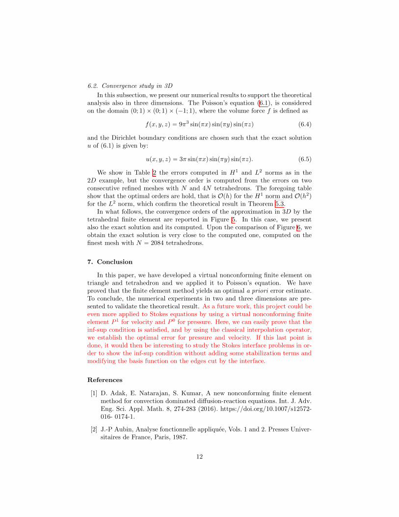
7. Conclusion

In this paper, we have developed a virtual nonconforming finite element ontriangle and tetrahedron and we applied it to Poisson’s equation. We haveproved that the finite element method yields an optimal a priori error estimate.To conclude, the numerical experiments in two and three dimensions are pre-sented to validate the theoretical result. As a future work, this project could beeven more applied to Stokes equations by using a virtual nonconforming finiteelement P 1 for velocity and P

0 for pressure. Here, we can easily prove that theinf-sup condition is satisfied, and by using the classical interpolation operator,we establish the optimal error for pressure and velocity. If this last point isdone, it would then be interesting to study the Stokes interface problems in or-der to show the inf-sup condition without adding some stabilization terms andmodifying the basis function on the edges cut by the interface.

References

[1] D. Adak, E. Natarajan, S. Kumar, A new nonconforming finite elementmethod for convection dominated di↵usion-reaction equations. Int. J. Adv.Eng. Sci. Appl. Math. 8, 274-283 (2016). https://doi.org/10.1007/s12572-016- 0174-1.

[2] J.-P Aubin, Analyse fonctionnelle appliquee, Vols. 1 and 2. Presses Univer-sitaires de France, Paris, 1987.

12

[3] M. Bachar, A. Guessab, A simple necessary and su�cient condition for theenrichment of the Crouzeix-Raviart element. Appl. Anal. Discrete Math.10 (2016), no. 2, 378-393.

[4] G.A. Baker, Finite element methods for elliptic equations using noncon-forming finite elements. Math. Comp. 1977, 31(137), 45-59.

[5] S. C. Brenner, R. L. Scott, The mathematical theory of finite elementmethods. Springer Sc. & Bus. Media, Vol. 15, 2007.

[6] P. G. Ciarlet, The finite element method for elliptic problems, North- Hol-land, Amsterdam, 1978.

[7] P. Ciarlet, Jr., C. F. Dunkl, S. A. Sauter, A Family of Crouzeix-Raviart Finite Elements in 3D. Anal. and Appl. (2017), 16,10.1142/S0219530518500070.

[8] M. Crouzeix, P.-A. Raviart, Conforming and nonconforming finite elementmethods for solving the stationary Stokes equations. I. Rev. Fr. Autom.,Inf. Rech. Oper. Math., 1973, 7(3): 33-75.

[9] A. Ern, J.-L. Guermond, Theory and practice of finite elements. Series:Applied Mathematical Sciences. Vol. 159, Springer, 2004.

[10] B.P. Lamichhane, A nonconforming finite element method for the Stokesequations using the Crouzeix-Raviart element for the velocity and the stan-dard linear element for the pressure. Int. J. Numer. Meth. Fluids, (2014)74: 222-228. doi:10.1002/fld.3848.

[11] R. Lim, D. Sheen, Nonconforming Finite Element Method Applied to theDriven Cavity Problem. Comput. Phys. Commun., (2017) 21(4), 1012-1038.doi:10.4208/cicp.OA-2016-0039.

[12] R.S. Falk, Nonconforming finite element methods for the equations of linearelasticity, Math. Comp., 57 (1991) 529-550.

[13] J. Hu, R. Ma, The Enriched Crouzeix-Raviart Elements are Equiva-lent to the Raviart-Thomas Elements. J Sci Comput 63, 410-425 (2015),https://doi.org/10.1007/s10915-014-9899-9.

[14] K. Kobayashi, T. Tsuchiya, Error analysis of Crouzeix-Raviart and Raviart-Thomas finite element methods. Japan J. Indust. Appl. Math. 35, 1191-1211 (2018). https://doi.org/10.1007/s13160-018-0325-9.

[15] D. Shi, L. Pei, Nonconforming quadrilateral finite element method for aclass of nonlinear sine-Gordon equation, Appl. Math. and Comput. 219(2013) 9447-9460.

[16] D. Shi, L. Wang, X. Liao, Nonconforming finite element analysis for poi- soneigenvalue problem, Computers and Math. with Appl., Volume 70, Issue 5,835-845, (Sept. 2015).

13

[17] D. Shi, H.Wang, The Crouzeix-Raviart type nonconforming finiteelement method for the nonstationary Navier-Stokes equations onanisotropic meshes. Acta Math. Appl. Sin. Engl. Ser. 30, 145-156 (2014),https://doi.org/10.1007/s10255-014-0274-2.

[18] B. Ayuso de Dios, K. Lipnikov, G. Manzini, The nonconforming virtual ele-ment method, ESAIM Math. Model. Numer. Anal., 50 (2016), pp. 879–904.

[19] A. Cangiani, G. Manzini, O.J. Sutton, Conforming and nonconformingvirtual element methods for elliptic problems. IMA J. Numer. Anal. 37(2016), 1317-1354.

[20] X. Liu, Z. Chen, The nonconforming virtual element method forthe Navier-Stokes equations. Adv. Comput. Math. 45, 51–74 (2019).https://doi.org/10.1007/s10444-018-9602-z.

[21] X. Liu, J. Li, Z. Chen, A nonconforming virtual element method for theStokes problem on general meshes, Comput. Method. Appl. M., 320 (2017),pp. 694–711.

[22] L. Beirao da Veiga, C. Lovadina, D. Mora, A virtual element method forelastic and inelastic problems on polytope meshes, Comput. Method. Appl.M., 295 (2015), pp. 327–346.

[23] A. Cangiani, V. Gyrya, G. Manzini, The nonconforming virtual elementmethod for the Stokes equations, SIAM J. Numer. Anal., 54 (2016), pp.3411–3435.

[24] A. Cangiani, G. Manzini, and O. J. Sutton, Conforming and nonconformingvirtual element methods for elliptic problems, IMA J. Numer. Anal., 37(2017), pp. 1317–1354.

[25] A. L. Gain, C. Talischi, G. H. Paulino, On the virtual element methodfor three-dimensional linear elasticity problems on arbitrary polyhedralmeshes., Comput. Method. Appl. M., 282 (2014), pp. 132–160.

[26] B. Zhang, J. Zhao, Y. Yang, S. Chen., The nonconforming vir-tual element method for elasticity problems, J. Comput. Phys. (2018),https://doi.org/10.1016/j.jcp.2018.11.004

[27] H. El-Otmany, Approximation par la methode NXFEM des problemesd’interface et d’interphase dans la mecanique des fluides, PhD thesis, Uni-versity of Pau, 2015.

14

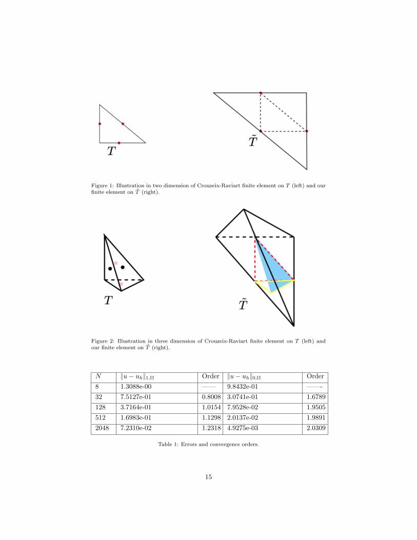
Figure 1: Illustration in two dimension of Crouzeix-Raviart finite element on T (left) and ourfinite element on T (right).

Figure 2: Illustration in three dimension of Crouzeix-Raviart finite element on T (left) andour finite element on T (right).

N }u ´ uh}1,⌦ Order }u ´ uh}0,⌦ Order

8 1.3088e-00 —— 9.8432e-01 ——-

32 7.5127e-01 0.8008 3.0741e-01 1.6789

128 3.7164e-01 1.0154 7.9528e-02 1.9505

512 1.6983e-01 1.1298 2.0137e-02 1.9891

2048 7.2310e-02 1.2318 4.9275e-03 2.0309

Table 1: Errors and convergence orders.

15

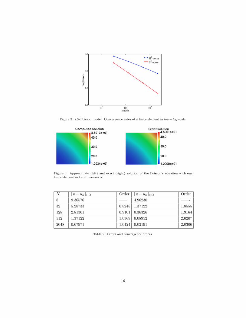
Figure 3: 2D-Poisson model: Convergence rates of a finite element in log ´ log scale.

Figure 4: Approximate (left) and exact (right) solution of the Poisson’s equation with ourfinite element in two dimensions.

N }u ´ uh}1,⌦ Order }u ´ uh}0,⌦ Order

8 9.36576 —— 4.96230 ——-

32 5.28733 0.8248 1.37122 1.8555

128 2.81361 0.9101 0.36326 1.9164

512 1.37122 1.0369 0.08952 2.0207

2048 0.67971 1.0124 0.02191 2.0306

Table 2: Errors and convergence orders.

16

Figure 5: 3D-Poisson model: Convergence rates of a finite element in log ´ log scale.

Figure 6: Approximate (left) and exact (right) solution of the Poisson’s equation with ourfinite element in three dimensions.

17