scuola superiore iuss - ucl.ac.ukucahmca/publications/theses/iuss_msc.pdf · matteo capoferri. 4....
TRANSCRIPT
Scuola Superiore IUSS
Classe Accademica di Scienze e Tecnologie
Corso di Laurea Magistrale in Scienze Fisiche
A Microlocal-Analytic Approachto the Propagator of the Wave Operator
Relatore:
Prof. Dmitri Vassiliev
Correlatore:
Prof. Claudio Dappiaggi
Tesi di Licenza dell’Allievo
Dott. Matteo Capoferri
Anno Accademico 2015-2016


.
Acknowledgements
I owe a debt of gratitude to my supervisor, prof. Dmitri Vassiliev, for intro-
ducing me to the subject and for devoting time and energies to stimulating
discussions and careful supervision.
Special thanks go to Claudio Dappiaggi, my co-supervisor, whose unfailing
encouragement is always source of renewed enthusiasm.
Lastly, I would like to acknowledge the support of the Mathematics Depart-
ment of University College London, where this work has been done.
London, 11 April 2017
Matteo Capoferri

4

Contents
Introduction 7
1 Preliminaries and notation 111.1 Oscillatory integrals . . . . . . . . . . . . . . . . . . . . . . . . 121.2 Fourier Integral Operators . . . . . . . . . . . . . . . . . . . . 151.3 Pseudo-Di↵erential Operators . . . . . . . . . . . . . . . . . . 16
1.3.1 Classical symbols . . . . . . . . . . . . . . . . . . . . . 211.3.2 DOs on manifolds . . . . . . . . . . . . . . . . . . . . 221.3.3 Principal and sub-principal symbol . . . . . . . . . . . 26
1.4 Hamiltonian flow . . . . . . . . . . . . . . . . . . . . . . . . . 281.4.1 Properties of the geodesic flow . . . . . . . . . . . . . . 30
1.5 Scalar functions versus half-densities . . . . . . . . . . . . . . 30
2 Global oscillatory integrals 332.1 The phase function revisited . . . . . . . . . . . . . . . . . . . 34
3 Construction of the propagator 373.1 Outline of the method . . . . . . . . . . . . . . . . . . . . . . 373.2 Solution for small times . . . . . . . . . . . . . . . . . . . . . 403.3 The complex-valued phase function . . . . . . . . . . . . . . . 42
3.3.1 A concrete example: the 2-sphere . . . . . . . . . . . . 453.4 The problem in perspective . . . . . . . . . . . . . . . . . . . 51
A Taylor expansions in normal geodesic coordinates 55
B Weyl coe�cients: a comparison 59
C An insight into amplitude reduction 63
Bibliography 65
5

6 Contents

Introduction
The study of the wave operator
P =@2
@t2��,
first introduced in the seventeenth century in the Euclidean setting, has at-tracted over the years the attention of researchers from the most diverseareas, due to its vast range of applications. Even though at first glance itmay look like a fairly easy operator, a careful analysis reveals that, underthe surface, it possesses very deep, far-reaching properties, which go beyondthe mere description of the propagation of waves. This can be intuitively un-derstood if we observe that it contains the Laplace-Beltrami operator ��,which is known to detect and encode information on the geometric structureof the space it acts upon.
When dealing with the wave operator P , it is often of particular interestto examine its propagator U(t), i.e. the one-parameter family of operators
U(t) : C1(M) ! C1(R⇥M),
satisfying
P U(t)f0 = 0.
If M is a closed Riemannian manifold, i.e. compact without boundary, thepropagator can be constructed in a semi-explicit way resorting to the L2-decomposition of the initial value f0 with respect to the orthonormal basisof the eigenfunctions of the Laplace-Beltrami operator. In fact, let �2
k
be theeigenvalues of �� and let v
k
be the corresponding orthonormalized eigen-functions. The function f0 can be written as
f0(x) =1X
k=0
vk
(x)
Z
M
[vk
(y)]⇤ f0(y) dVolM =1X
k=0
ak
vk
(x).
7
8 Contents
Then, the propagator is given by
U(t)f0(x) = e�i t
p�� f0(x) =
1X
k=0
e�i t�
k vk
(x)
Z
M
[vk
(y)]⇤ f0(y) dVolM .
The reason for which this construction is semi-explicit and not actually ex-plicit, is that, made exception for a few special cases, the eigenvalues and theeigenfunctions of �� for a generic Riemannian manifold are not known.
In order to overcome this issue, we will pursue a di↵erent strategy to theend of approximating the propagator U(t) with a Fourier integral operator.The extent of the approximation is twofold. On the one hand, the symbolof the oscillatory integral we will construct is unique up to smooth terms;this means that it succeeds in fully capturing the singular structure of thepropagator, but it coincides with U(t) modulo a smoothing operator only.On the other hand, the procedure we adopt in reconstructing the amplituderelies on a hierarchy of equations which have to be solved one after the otherto obtain positively homogeneous components of subsequently decreasingorder. We will be interested in studying the first two non-trivial instances ofsuch equations, so as to eventually end up with an explicit formula for thesubleading contribution to the full symbol.
In doing this, we will exploit techniques developed by Safarov and Vas-siliev in [SV96] and [LSV94]. It is worth observing from the very beginningthat, besides being fully explicit, their algorithm allows for a constructionthat is global in time, due to the use of a non-degenerate, complex-valuedphase function. This is, in general, not possible with a real-valued phasefunction because of obstructions originating from the presence of caustics.
As the research is still ongoing, we will not be able to present in ourthesis a full-fledged solution to the problem. Rather, we will formulate itin mathematically precise terms and we will discuss some explicit examples.This will shed light on the construction algorithm and will provide an insighton where the di�culties lie. At the very end, we will make some commentson possible strategies to tackle the problem in the general case.
After having sketched out the framework and motivated the problemwe are going to deal with, let us briefly outline the content of the thesis,articulated into three chapters.
In Chapter 1 we introduce set-up and notation and we present the math-ematical tools needed in the following, with particular attention to the prop-erties of oscillatory integrals and of Hamiltonian flows.
Chapter 2 is mainly concerned with further elaboration on oscillatory

Contents 9
integrals, with a focus on their global properties. Complex-valued phasefunctions are introduced in this chapter.
Chapter 3 represents the original part of our work. After an outline ofthe method, the small-times approximation for a real-valued phase functionis discusses, showing that the adopted approach gives results fully consis-tent with those obtained through other methods (e.g. heat kernel methods).Subsequently, structure and properties of a particular complex-valued phasefunction are analysed, along with the derivation of some useful formulae. Inthe case of the 2-sphere, computations are carried out explicitly, showingthat degeneracy is removed for all times. In the end, additional formulae arediscussed in perspective.
Further material and calculations have been included in Appendix A,Appendix B and Appendix C.

10 Contents
Chapter 1
Preliminaries and notation
In this first chapter we will introduce some definitions and we will establishthe notation that will be used throughout the thesis. In doing this, we willrecall and prove a certain number of well-established properties and resultsregarding the mathematical objects involved, for later use.
Definition 1.1. We call ↵ a multi-index if it is an element ↵ 2 Nk
0 for somek 2 N. In other words, ↵ = (↵1, . . . ,↵k
) is an k�vector whose componentsare natural numbers.
Let x = (x1, . . . , xn
) 2 Rn. We adopt the following notation:
@i
=@
@xi
, j = 1, . . . , n,
@↵ = @↵11 · · · @↵n
n
=@|↵|
@↵11 · · · @↵n
n
,
where the modulus of a multi-index is defined as |↵| :=P
n
i=1 ↵i
. We will write@x
i and @↵x
instead of @i
and @↵ when it is not obvious with respect to whichvariable we are di↵erentiating. Furthermore, we denote by h⇠ , xi := ⇠i x
i
thestandard inner product in Rn.
Unless otherwise specified, we adopt the Einstein convention on repeatedindices.
We recall the definition of some important functional spaces:
C1(X): It is the Frechet space of infinitely di↵erentiable functions f on a do-main X ✓ Rn;
11
12 1. Preliminaries and notation
C10 (X): It is the locally convex vector space of infinitely di↵erentiable functions
f on a domain X ✓ Rn with compact support:
supp(f) ⇢⇢ X;
S(Rn): It is the Frechet space of infinitely di↵erentiable functions f decreasingat infinity faster than any power of |x|:
supx
|x↵ @�f(x)| < +1, 8↵, � 2 Nn
0 ;
L2(X,µ): It is the Hilbert space of square integrable functions f on a X withrespect to the measure µ:
kfk22 :=Z
X
|f(x)|2 dµ < +1.
When it is clear from the context with respect to which measure weare integrating, we drop the second entry and we write L2(X).
D0(X): It is the space of distributions, i.e. continuous linear functionals T :C1
0 (X) ! R;
S 0(X): It is the space of tempered distributions, i.e. continuous linear function-als T : S(X) ! R.
1.1 Oscillatory integrals
Consider the following integral:
I'
(au) =
ZZei'(x,⇠) a(x, ⇠) u(x) dx d⇠. (1.1)
The aim of this section is to study its properties under suitable assump-tions on ', a and u. Fistly, let us introduce two classes of functions whichlay the foundations for a rigorous regularisation of (1.1).
Definition 1.2 (Symbols). Let X be an open subset of Rn, m 2 R and(�, ⇢) 2 [0, 1] ⇥ [0, 1]. The space Sm
⇢,�
(X ⇥ RN) of symbols of order m⇢,�
consists of functions a 2 C1(X ⇥ RN) such that for every multi-indices↵ 2 Nn
0 , � 2 NN
0 and for every compact set K ⇢ X there exists a constantC
↵,�,K
2 R>0 such that:
|@↵✓
@�⇠
a(x, ⇠)| C↵,�,K
(1� |⇠|)m�⇢|↵|+�|�| 8x 2 K, 8⇠ 2 RN . (1.2)
When (⇢, �) = (1, 0), we write Sm(X ⇥ RN) instead of Sm
1,0(X ⇥ RN). Fur-thermore, we define S�1 :=
Tm
Sm(X ⇥ RN).
1.1 Oscillatory integrals 13
Definition 1.3 (Phase function). With the same notation as above, we call' a phase function if it satisfies the properties:
(i) ' 2 C1(X ⇥ RN \ {0});
(ii) '(x, t⇠) = t'(x, ⇠) for every t 2 R>0, i.e. ' is positively homogeneous
in ⇠ of degree 1;
(iii) gradx,⇠
' 6= 0 for all (x, ⇠) 2 X ⇥RN \ {0}, i.e. ' does not have criticalpoints outside {(x, 0) | x 2 X}.
Whenever ' is a phase function, a is a symbol and u is an element inC1
0 (X) the integral (1.1) is called oscillatory integral.The integral (1.1) is not, in general, absolutely convergent. The following
lemma, whose meaning will be clear soon, o↵ers a way of regularising it.
Lemma 1.4 ([Shu87, Lemma 1.1]). Let X be an open domain in Rn. Thereexists a di↵erential operator on C1
0 (X ⇥ RN)
P = aj
(x, ⇠)@⇠
j
+ bk
(x, ⇠) @x
k
+ c(x, ⇠) (1.3)
with coe�cients aj
2 S01,0(X⇥RN), b
k
2 S�11,0(X⇥RN) and c 2 S�1
1,0(X⇥RN)such that
tP�ei'
�= ei', (1.4)
where the formal transposed operator tP is given, for u 2 C10 (X ⇥ RN), by:
tPu = �@⇠
j
(aj
u)� @x
k
(bk
u) + cu.
Proof. Define:
f(x, ⇠) :=
NX
i=1
|⇠|2����@'
@⇠i
����2
+nX
j=1
����@'
@xj
����2!�1
.
We drop, along the proof, the argument (x, ⇠) when there is no confusion,for the sake of clarity. One immediately realises that f 2 C1(X⇥RN \{0}),in view of the fact that the phase function can not be singular for ⇠ 6= 0. fis positively homogeneous in ⇠ of degree �2 and it satisfies:
�if
NX
i=1
|⇠|2 @'@⇠
i
@
@⇠i
+nX
j=1
@'
@xj
@
@xj
!ei' = ei'.
14 1. Preliminaries and notation
We are close to finding a promising candidate for tP ; we only need to curethe potential singularity of f at ⇠ = 0. Pick a bump function ✓ 2 C1
0 (Rn)such that:
✓(⇠) =
(1 for |⇠| < 1/2
0 for |⇠| > 1,
and put:
tP = �i f (1� ✓)
NX
i=1
|⇠|2 @'@⇠
i
@
@⇠i
+nX
j=1
@'
@xj
@
@xj
!+ ✓.
It is a straightforward check that the formal transposition is involutive; hence,the operator P := t(tP ) possesses the required properties, where:
aj
= i f (1� ✓) |⇠|2 @'@⇠
j
,
bk
= i f (1� ✓)@'
@xk
,
c = �NX
j=1
@aj
@⇠j
�nX
k=1
@bk
@xk
+ ✓.
(1.5)
We are now in a position to return to the oscillatory integral. To beginwith, we observe that if the symbol a is of degree m
⇢,�
< �N , then (1.1) iswell-defined and absolutely convergent. If this is not the case, we exploit theoperator P built above. Integrating k times by parts we obtain:
I'
(au) =
ZZei'a u dx d⇠
=
ZZ(tP )k(ei') a u dx d⇠
=
ZZei' P k(au) dx d⇠.
Now, we can safely a�rm that P k(au) 2 Sm�k[min{⇢,1��}]. If � > 0 and⇢ < 1, then s := min{⇢, 1 � �} > 0; we can choose k big enough, so thatm� ks < �N , making the integral absolutely convergent.
Remark 1.5. There is a way of regularising the oscillatory integral also inthe case of symbols in Sm
1,�(X ⇥ RN) or in Sm
⇢,0(X ⇥ RN). See, for instance,[Hor85].

1.2 Fourier Integral Operators 15
The oscillatory integrals induce the following maps, continuous with re-spect to the relevant topologies:
• For fixed ' and a,
A : C10 (X) !R,
u 7! hA , ui := I'
(au)
defines a distribution in D0(X).
An estimate of the singular support of the distribution A is capturedby the singular set of ':
C'
:= {(x, ⇠) 2 X ⇥ RN \ {0} | grad⇠
'(x, ⇠) = 0}. (1.6)
It is easy to see that sing suppu ✓ ⇡(C'
), where ⇡ : X ⇥ RN ! X isthe canonical projection onto the first component.
• For fixed ' and u, I'
( · u) : Sm
⇢,�
(X ⇥ RN) ! R defines a continuouslinear functional on the Frechet space Sm
⇢,�
(X ⇥ RN).
From this perspective, the regularisation of an oscillatory integral isnothing but an extension by continuity of the above linear functionalfor increasing degree m; in fact, it is possible to check that the closureof S�1 in Sm
⇢,�
(X ⇥ RN) contains Sm
0⇢,�
(X ⇥ RN) for m0 < m.
1.2 Fourier Integral Operators
Definition 1.6. Let X ✓ Rn, Y ✓ Rn
0, ' be a phase function and a 2
Sm
⇢,�
(X ⇥ Y ⇥ RN), with ⇢ 6= 1 and � 6= 0. We call Fourier Integral Operator(FIO) a linear map
A : C10 (Y ) ! D0(X)
u 7! Au (1.7)
where A is defined by:
Au(x) =1
(2⇡)n
ZZei'(x,y,⇠) a(x, y, ⇠) u(y) dy d⇠. (1.8)
Remark 1.7. The factor (2⇡)�n in (1.8) is not always present in the standardliterature: we adopt it here merely for a matter of computational convenience,as will be clear in what follows.

16 1. Preliminaries and notation
Observe that if we integrate Au against a smooth, compactly supportedfunction v 2 C1
0 (X), we obtain an ordinary absolutely convergent oscillatoryintegral on eX ⇥ RN , where eX = X ⇥ Y ✓ Rn ⇥ Rn
0:
hAu , vi = 1
(2⇡)n
ZZZei'(x,y,⇠) a(x, y, ⇠) u(y) v(x) dx dy d⇠.
Definition 1.8. We call kernel of the operator A the distribution KA
2D0(X ⇥ Y ) whose integral kernel is given by:
KA
(x, y) =1
(2⇡)n
Zei'(x,y,⇠) a(x, y, ⇠) d⇠.
We will return to Fourier Integral Operators later in Chapter 2, discussingadditional regularity requirements which can be made for the phase functionand the the structure of its singularities.
1.3 Pseudo-Di↵erential Operators
There is a distinguished class of FIOs, of great importance and with vastapplications, characterised by a specific choice of the functional form of thephase function:
Definition 1.9. Let X = Y ✓ Rn, a 2 Sm
⇢,�
(X ⇥ Rn) and let the phasefunction be '(x, y, ⇠) = hx � y , ⇠i. We call Pseudo-Di↵erential Operator( DO) a FIO A : C1
0 (X) ! C1(X) of the form:
Au(x) =1
(2⇡)n
ZZeihx�y , ⇠i a(x, y, ⇠) u(y) dy d⇠. (1.9)
The class of pseudo-di↵erential operators defined by symbols a 2 Sm
⇢,�
(X ⇥X⇥Rn) of order m
⇢,�
is denoted by Lm
⇢,�
(X). We put L�1(X) =T
m
Lm
1,0(X).
Remark 1.10. Note that, unlike a general FIO, the range of a DO A liesin the subspace C1(X) ⇢ D0(X). This is due to the automatic fulfilment ofthe non-degeneracy conditions:
gradx,⇠
'(x, y, ⇠) 6= 0 for (x, y, ⇠) 2 Rn ⇥ Rn ⇥ (Rn \ {0}), (1.10a)
grady,⇠
'(x, y, ⇠) 6= 0 for (x, y, ⇠) 2 Rn ⇥ Rn ⇥ (Rn \ {0}). (1.10b)
See [Shu87, Proposition 2.2] for additional details.

1.3 Pseudo-Di↵erential Operators 17
As above, by Schwartz kernel theorem [Hor83, Theorem 5.2.1] we canassociate to the map:
A : C10 (X) ! D0(X)
u 7! Au
a distribution KA
2 D0(X ⇥ X). KA
is called the kernel of the pseudo-di↵erential operator A. We denote by K
A
(x, y) the integral kernel of KA
.
Proposition 1.11. Let A be a DO. Then A extends by continuity to alinear map:
A : E 0(X) ! D0(X).
Observe that, unlike linear di↵erential operators, DOs do not enjoy thelocality property, i.e. it is not guaranteed that suppAu ✓ supp u for u 2C1
0 (X). Rather, DOs are pseudolocal, namely sing suppAu ✓ sing supp ufor every u in E 0(X). In other words, DOs may enlarge the support of thedistribution they act upon, but they can not worsen its regularity.
Definition 1.12. Let A be a DO. The transposed operator tA is definedby:
Z(Au)(x) v(x) dx =
Zu(x)
�tAv
�(x) dx, 8u, v 2 C1
0 (X).
If A 2 Lm
⇢,�
(X), it is an easy check that also tA 2 Lm
⇢,�
(X). As a matterof fact, writing A as per equation (1.9), with a 2 Sm
⇢,�
(X ⇥ Rn), we have:
tAv(x) =1
(2⇡)n
ZZeihy�x , ⇠i a(x, y,�⇠) v(x) dx d⇠, (1.11)
from which the claim follows.
Definition 1.13 (Full symbol). Let A be a DO. The function:
�A
: X ⇥ Rn ! C(x, ⇠) 7! e�ihx , ⇠i �Aeih· , ⇠i
�(x)
is called full symbol of A.
In terms of the full symbol, a pseudo-di↵erential operator A takes theform:
Au(x) =1
(2⇡)n
Zeihx , ⇠i �
A
(x, ⇠) u(⇠) d⇠, (1.12)

18 1. Preliminaries and notation
where ˆ denotes the Fourier transform. A closer look at equations (1.12) and(1.9) reveals that the full symbol �
A
can be expanded as:
�A
(x, ⇠) =1
(2⇡)n
ZZe�ihz , ⌘i a(x, x+ z, ⇠ + ⌘) dz d⌘. (1.13)
If we are interested in investigating problems in which the singular struc-ture of the operator is the only thing that matters, we can then restrict ouranalysis to a subclass of DOs, namely the properly supported DOs.
Definition 1.14. A pseudo-di↵erential operator A is properly supported ifthe projection maps:
⇡1 : suppKA
! X
(x, y) 7! x,⇡2 : suppKA
! X
(x, y) 7! y,
are proper.
In fact, an arbitrary DO A can be decomposed as A = A + A0, whereA is properly supported and A0 is a smoothing operator [Hor85, Proposition18.1.22]. This means that properly supported operators capture all informa-tion concerning the singularities of DOs. What is more, properly supported DOs are much easier to handle from a technical perspective in proofs andcomputations, in view of the fact that they map C1
0 (X), C1(X), D0(X) andE 0(X) into themselves continuously.
In the properly supported case, it makes complete sense to consider thecomposition of two pseudo-di↵erential operators. Composition, in general,does not induce a homomorphism at the level of symbols; this holds true, aswe shall see in the following, only for the principal symbol, i.e. the leadingorder term of the full symbol. Before discussing composition, let us introducebriefly the notion of asymptotic expansion.
Definition 1.15. Let {mk
} be a real sequence such that limk!1 m
k
= �1.Furthermore, let a
k
2 Sm
k
⇢,�
(X ⇥ Rn) for every k 2 N and a 2 C1(X ⇥ Rn).We write:
a ⇠1X
k=1
ak
(1.14)
if
a�s�1X
k=1
ak
2 Sm
s
⇢,�
(X ⇥X ⇥ Rn)
for every s � 2, where ms
= maxk�s
mk
.

1.3 Pseudo-Di↵erential Operators 19
The following proposition makes it easier to verify whether a given asymp-totic expansion holds:
Proposition 1.16 ([Shu87, Proposition 3.6]). Let a 2 C1(X ⇥ Rn) suchthat for every compact set K ✓ X and for every multi-indices ↵, � 2 Nn
0
there exist constants � and C such that:
|@↵x
@�⇠
a(x, ⇠)| C (1 + |⇠|)�, 8x 2 K. (1.15)
Moreover, let {ak
} be as in Definition 1.15. Then the following are equivalent:
(i) a ⇠P1
k=1 ak;
(ii) For every compact subset K ⇢ X there exists a sequence {�s
} such thatlim
s!1 �s
= �1 and�����a(x, ⇠)�
s�1X
k=1
ak
(x, ⇠)
����� Cs
(1 + |⇠|)�s , 8x 2 K, (1.16)
for some constants {Cs
}.
The previous statement proves extremely useful in establishing the fol-lowing fundamental result:
Proposition 1.17. Let A 2 Lm
⇢,�
(X) be a properly supported DO, let �A
beits symbol and define D↵ := �i@↵. Then:
�A
(x, ⇠) ⇠X
↵2Nn
0
1
↵!@↵⇠
D↵
y
a(x, y, ⇠)|y=x
. (1.17)
Remark 1.18. Sometimes (cfr. [Hor85]) the above result is expressed moreconcisely and e↵ectively as:
�A
(x, ⇠) ⇠ eihDy
, D
⇠
i a(x, y, ⇠)|y=x
.
An analogous result ensues for the full symbol of the transposed operator:
Corollary 1.19. Let A be a properly supported DO and let �A
be its fullsymbol. Then, the full symbol �0
A
of the transposed operator tA admits theexpansion:
�0A
(x, ⇠) ⇠X
↵2Nn
0
1
↵!@↵⇠
D↵
x
�A
(x,�⇠). (1.18)
We are now in a position to state and prove the composition theorem.
20 1. Preliminaries and notation
Theorem 1.20 (Composition theorem). Let A 2 Lm1⇢,�
(X) and B 2 Lm2⇢,�
(X)be properly supported DOs with (full) symbols �
A
and �B
respectively. Then,the operator C = B � A is a properly supported DO in Lm1+m2
⇢,�
(X). Fur-thermore, its full symbol admits the following asymptotic expansion:
�C
(x, ⇠) ⇠X
↵2Nn
0
1
↵!@↵⇠
�B
(x, ⇠)D↵
x
�A
(x, ⇠). (1.19)
Proof. In view of the fact that:
tAu(x) =1
(2⇡)n
ZZeihx�y , ⇠i �
A
(y,�⇠) v(y) dy d⇠,
and observing that the transposition is involutive, A can be expressed as:
Au(x) = t(tA)u(x) =1
(2⇡)n
ZZeihx�y , ⇠i �0
A
(y,�⇠) u(y) dy d⇠,
and its Fourier transform is given by:
cAu(⇠) =Z
e�ihy , ⇠i�0A
(y,�⇠)u(y)dy.
Consequently, the action of B on Au reads:
Cu(x) = B(Au)(x) =1
(2⇡)n
ZZeihx�y , ⇠i �
B
(x, ⇠) �0A
(y,�⇠) u(y) dy d⇠.
(1.20)From the product of symbols in the above equations it ensues that C =B � A 2 Lm1+m2
⇢,�
(X) is properly supported.
As far as the asymptotic expansion is concerned, we have, using Propo-sition 1.17:
�C
(x, ⇠) ⇠X
↵2Nn
0
1
↵!@↵⇠
D↵
y
(�B
(x, ⇠) �0A
(y,�⇠)) |y=x
⇠X
↵2Nn
0
1
↵!@↵⇠
D↵
y
2
4�B
(x, ⇠)
0
@X
�2Nn
0
(�1)|�|
�!@�⇠
D�
⇠
�A
(y, ⇠)
1
A
3
5
������y=x
.
1.3 Pseudo-Di↵erential Operators 21
Invoking the Leibniz rule for multi-indices, we get:
�C
(x, ⇠) ⇠X
↵,�2Nn
0
(�1)|�|
�!
X
�+�=↵
1
�!�!
⇥@�⇠
�B
(x, ⇠)⇤ h@�+�
⇠
D↵+��A
(x, ⇠)i
=X
�,�,�2Nn
0
(�1)|�|
�!�!�!
⇥@�⇠
�B
(x, ⇠)⇤ h@�+�
⇠
D�+�+��A
(x, ⇠)i
=X
�2Nn
0
1
�!
X
2Nn
0
X
�+�=
(�1)|�|
�!�!
!⇥@�⇠
�B
(x, ⇠)⇤ ⇥@⇠
D�+�A
(x, ⇠)⇤.
(1.21)
Define e := (1, 1, . . . , 1) 2 Rn; by virtue of the Newton multinomial formulathe following identity holds:
(e+ (�e)) =X
�+�=
!
�!�!e� (�e)� = !
X
�+�=
(�1)|�|
�!�!=
(1 if || = 0
0 if || > 0.
Therefore, the only non-vanishing contribution to the inner summation inthe last step of (1.21) is the one for || = 0. Eventually, we obtain
�C
(x, ⇠) ⇠X
�2Nn
0
1
�!@�⇠
�B
(x, ⇠)D�
x
�A
(x, ⇠),
which concludes the proof.
Remark 1.21. Again, the above theorem can be reformulated formally in amore concise way (cfr. [Hor85]) as
�C
(x, ⇠) ⇠ eihD⌘
, D
y
i �A
(x, ⌘)�B
(y, ⇠) |⌘=⇠,y=x
.
1.3.1 Classical symbols
In a certain number of problems, it is often convenient to consider a subclassof the class of symbols: the classical symbols.
Definition 1.22. LetX be an open domain in Rn. We say that a is a classicalsymbol of degree m and we write a 2 CSm(X ⇥ RN) if a 2 C1(X ⇥ RN)and it admits the asymptotic expansion:
a ⇠1X
j=0
(⇠) am�j
(x, ⇠), (1.22)
22 1. Preliminaries and notation
where am�j
is positively homogeneous in ⇠ of degree m� j and 2 C1(RN)is such that:
(⇠) =
(0 |⇠| 1/2
1 |⇠| � 1.
We denote by CLm(X) the class of DOs that can be written in the form(1.9) with a 2 CSm(X ⇥X ⇥ Rn).
From Definition 1.22, it follows that CSm(X) ✓ Sm
1,0(X). Furthermore,if we restrict to properly supported operators, it is a straightforward conse-quence of the formulae presented above
• that the full symbol of a classical DO is a classical symbol in the senseof Definition 1.22,
• that the composition of classical DOs yields a classical DO and
• that the transposed and the adjoint of a classical DO are classical DO.
Hence, the space of classical DOs turns out to be a sensible subclass, stableunder the most important operations. In the next section, we will show thatit is also closed under change of coordinates.
1.3.2 DOs on manifolds
Let us now discuss the properties of DOs under change of coordinates. LetX, eX ✓ Rn be open sets and let : X ! eX be a di↵eomorphism. inducesan isomorphism ⇤ : C1( eX) ! C1(X), u 7! ⇤u := u � . We observe that⇤ maps compactly supported functions to compactly supported functions.
Let now A : C10 (X) ! C1(X) be a DO. We aim at defining a new
operator eA on eX, which we would like to interpret as the DO correspondingto A under the change of coordinates described by the di↵eomorphism . Wedefine eA as the operator:
eA := (⇤)�1 A⇤, (1.23)
eAu = [A(u � )] � �1
making the diagram
C10 (X) A // C1(X)
C10 ( eX)
⇤
OO
eA
// C1( eX)
⇤
OO(1.24)
1.3 Pseudo-Di↵erential Operators 23
commutative. We obtain:
eAu(x) = 1
(2⇡)n
ZZeih
�1(x)�y , ⇠i a(�1(x), y, ⇠) u((y)) dy d⇠
=1
(2⇡)n
ZZeih
�1(x)�
�1(z) , ⇠i a(�1(x),�1(z), ⇠) u(z)J dz d⇠,
(1.25)
where we we substituted y = �1(z) and we put J =
����det✓@y
@z
◆����.
Even though eA is evidently a FIO, it is not clear whether it is DO. Weknow that, given a FIO, the phase function and the symbol are not uniquelyassigned; following [Shu87], we will show that it is possible to perform a localchange of coordinate in the ⇠-space, so that the phase function h�1(x) ��1(y) , ⇠i is turned to a phase function of the form hx� y , ⌘i, thus making(1.25) a manifestly well-defined DO.
Proposition 1.23. Let ' be a phase function satisfying the additional con-ditions:
(a) '(x, y, ⇠) is linear in ⇠;
(b) grad⇠
'(x, y, ⇠) = 0 () (x, y) 2 �(X),
where �(X) denotes the diagonal {(x, x) 2 X ⇥ X}. Then there exists aneighbourhood ⌦ � �(X) and a map 2 C1(⌦;GL(n,R)) such that:
'(x, y, (x, y) ⇠) = hx� y , ⇠i, 8(x, y) 2 ⌦
and[det (x, x)] [det'
x
↵
⇠
�
(x, y, ⇠)��x=y
] = 1.
Proof. The assumption (a) tells us that, without loss of generality, the phasefunction can be written as:
'(x, y, ⇠) =nX
k=1
fk
(x, y) ⇠k
for some smooth functions fk
, k = 1, . . . , n. From (b) we deduce that the fk
smust fulfil
fk
(x, y) = 0 () x = y.
It follows that:'(x, x, ⇠) = 0;
24 1. Preliminaries and notation
hence, gradx
'(x, y, ⇠)|x=y
= � grady
'(x, y, ⇠)|x=y
. Since (iii) in Definition1.3 requires grad
x,y,⇠
'(x, y, ⇠) to be non-vanishing for ⇠ 6= 0, this constrainsgrad
x
'(x, y, ⇠)|x=y
to be non-zero. In other words, for every ⇠ 2 Rn \ {0}there exists j 2 {1, . . . , n} such that
nX
k=1
@fj
@xk
����x=y
⇠k
6= 0.
We can apply the Hadamard lemma, which guarantees the existence of aneighbourhood ⌦0 of �(X) such that:
fi
(x, y) =nX
k=1
f(k)i
(x, y)(x� y)k
, x, y 2 ⌦0,
where f(k)j
2 C1(⌦0) and
f(k)i
(x, x) =@f
i
(x, y)
@xk
����x=y
.
Furthermore, by continuity of the determinant, there exists a neighbourhood⌦ ✓ ⌦0 of the diagonal �(X) such that det(f (k)
i
(x, y)) 6= 0 for (x, y) 2 ⌦.Let F 2 C1(⌦, GL(n,R)) be the matrix-valued function whose components
are Fij
= f(j)i
. Define the smooth function:
: ⌦! GL(n,R)(x, y) 7! (x, y) := F (x, y)�1.
Then, for (x, y) 2 ⌦, we have:
'(x, y, (x, y)⇠) =nX
i,k,j=1
F (x, y)ik
(x, y)kj
⇠j
(x� y)i
= hx� y , F (x, y) (x, y) ⇠i= hx� y , ⇠i.
The condition on the determinant is automatically satisfied by our construc-tion.
Theorem 1.24. Let 1� ⇢ � < ⇢ and a 2 Sm
⇢,�
(X⇥X⇥Rn). Furthermore,let ' be a phase function on X ⇥X ⇥Rn satisfying (a) and (b) in Definition1.23. If A is a FIO with phase function ' and symbol a, then A 2 Lm
⇢,�
(X).
1.3 Pseudo-Di↵erential Operators 25
Proof. Without loss of generality, the statement follows if we prove it in thecase a = 0 outside an arbitrary neighbourhood ⌦ � �(X). Choosing ⌦ asin the thesis of the previous theorem and putting ⇠ = (x, y) ⌘ we have:
Au(x) =1
(2⇡)n
ZZeihx�y , ⌘i a(x, y, (x, y)⌘) | det (x, y)| u(y) dy d⌘.
By Lemma [Shu87, Lemma 1.2] we conclude that a1(x, y, ⇠) := a(x, y, (x, y)⇠)is a symbol in Sm
⇢,�
(X). This completes the proof.
We are now in a position to observe that the operator eA defined by (1.25)fulfils the hypotheses of Theorem 1.24; eA is, therefore, a well-defined DO.
As before, we can give an asymptotic expansion for the transformed sym-bol after the change of coordinates:
Proposition 1.25 ([Shu87, Theorem 4.2]). Let : X ! eX be a di↵eomor-phism and let A 2 Lm
⇢,�
(X) be a properly supported DO with 1� ⇢ � < ⇢.
Let eA be given by (1.23). Then the following asymptotic expansion holds:
� eA
(y, ⌘)��y=(x)
⇠X
↵2Nn
0
1
↵!�(↵)A
(x, t grad(x) ⌘)D↵
z
ei x
(z) ⌘��z=x
, (1.26)
where we denote x
(z) = (z) � (x) � grad(x) (z � x) and �(↵)A
(x, ⇠) =@↵⇠
�A
(x, ⇠).
Remark 1.26. We observe that the above asymptotic expansion is welldefined. In fact, as a consequence of
x
(z) having a second-order zero atz = x,
D↵
z
ei x
(z) ⌘��z=x
depends on ⌘ polynomially of a degree at most |↵|/2. All the higher orderterms vanish as soon as we set z = x. Furthermore, the same reasoningentails that the first non-zero term in the sum occurs for |↵| = 2.
At this stage we have at hand all the ingredients to introduce the notionof pseudo-di↵erential operators on manifolds. Let M be a smooth manifoldand consider a linear map:
A : C1(M) ! C10 (M).
For each chart (X,�), we can construct an analogue of diagram (1.24):
C10 (X)
A|X // C1(X)
C10 ( eX)
�
⇤
OO
eA
�
// C1( eX)
�
⇤
OO(1.27)

26 1. Preliminaries and notation
where A|X
denotes the canonical restriction of A to X, �⇤ the pull-back along�, eX is the di↵eomorphic image of X in Rn and eA
�
= (�⇤)�1 A|X
�⇤.
Definition 1.27. A linear operator A : C10 (M) ! C1(M) is called pseudo-
di↵erential operator on M if for every chart (X,�) the operator eA�
is apseudo-di↵erential operator on �(X). For 1 � ⇢ � < ⇢, we denote bySm
⇢,�
(T ⇤M) and Lm
⇢,�
(M) the classes of symbols and associated pseudo-di↵erentialoperators on M obtained by extending in the natural way the analogous def-initions from the Euclidean setting.
Theorem 1.25 guarantees that the above definition is sensible and consis-tent.
1.3.3 Principal and sub-principal symbol
In view of the above discussion, it is possible to associate with pseudo-di↵erential operators two very important invariantly defined objects: theprincipal and the sub-principal symbols.
Definition 1.28. Let A 2 Lm
⇢,�
(X), 1 � ⇢ � < ⇢. We call principalsymbol of the operator A the image �p of the full symbol �
A
in the quotient
Sm
⇢,�
(X ⇥ Rn)/Sm�2(⇢�1/2)⇢,�
(X ⇥ Rn).
Proposition 1.25 and Remark 1.26 entail that:
� eA
(y, ⌘)��A
(�1(y), [t grad(�1)(y)]�1 ⌘) 2 Sm
⇢,�
(X⇥Rn)/Sm�2(⇢�1/2)⇢,�
(X⇥Rn).
Hence, the principal symbol is a well-defined, invariant function on the cotan-gent bundle T ⇤X of X. In fact, given a di↵eomorphism : X ! eX, theprincipal symbol transforms according to:
�p((x), ⇠) = �p(x,t grad(x) ⇠), (1.28)
where �p
denotes the principal symbol of eA. We will show in the followingthat the principal symbol of an operator plays a crucial role in the study ofits asymptotic spectral properties.
In the case of classical operator A 2 CLm(X), ⇢ = 1 and the principalsymbol can be identified with the positively homogeneous function of highestdegree of homogeneity m:
�m
= am
2 CSm(X)/CSm�1(X).
The term after the first one in the asymptotic expansion, either forA 2 Lm
⇢,�
(X) or A 2 CLm(X), is, in general, not invariant under change of

1.3 Pseudo-Di↵erential Operators 27
coordinates and it is not, therefore, a well-defined geometric object. We can,nonetheless, introduce a covariant object combining the sub-leading term andthe principal symbol. Let us focus our attention on classical DOs.
Definition 1.29. Let A 2 CLm(X). We call sub-principal symbol of A thepositively homogeneous function of degree m� 1 defined by:
�sub(x, ⇠) = am�1(x, ⇠) +
i
2
nX
k=1
@x
k@⇠
k
�p
(x, ⇠). (1.29)
It is not di�cult to show that the sub-principal symbol is a well-definedfunction on the cotangent bundle (see [SV96, Sec. 2.1.3], [Hor85, Sec. 18.1]).If : X ! eX is a di↵eomorphism, then:
�sub((x), ⇠) = �sub(x,t grad(x) ⇠).
The principal and the sub-principal symbols define a DO A 2 CLm(X),modulo DOs of order m� 2. In particular, they completely characterise afirst-order di↵erential operator.
Remark 1.30. The definition of sub-principal symbol may look, at firstglance, artificial. However, the definition of sub-principal symbol becomesvery natural in the perspective of Weyl calculus, cfr. [Hor85, Sec. 18.6]. Infact, let A 2 CLm(X) and let:
a ⇠1X
k=0
am�k
be the asymptotic expansion of its symbol. Then, there exists B 2 CLm(X)with symbol
b ⇠1X
k=0
bm�k
,
such that A = Bw, where the superscript w denotes the Weyl quantisationof the operator, and
�p = bm
, �sub = bm�1.
The sub-principal symbol of A emerges then as the invariant sub-leading termof the asymptotic expansion of the symbol of the Weyl quantised operatorBw associated to A. See [Hor85] for further details.

28 1. Preliminaries and notation
1.4 Hamiltonian flow
Let M be a closed manifold, i.e. compact without boundary, equipped witha Riemannian metric. We call Hamiltonian the function on the cotangentbundle T ⇤M \ 0, defined in a local trivialisation by:
h(x, ⇠) =qgµ⌫(x) ⇠
µ
⇠⌫
. (1.30)
Observe that the Hamiltonian is a positively homogeneous function in ⇠ ofdegree 1. For t 2 R, we denote by (x⇤(t; y, ⌘), ⇠⇤(t; y, ⌘)) the Hamiltoniantrajectories, videlicet the solution to the Hamiltonian system:
8>><
>>:
x⇤↵ =@h
@⇠↵
(x⇤, ⇠⇤),
⇠⇤�
= � @h
@x�
(x⇤, ⇠⇤),
(1.31)
with initial conditions (x⇤(0; y, ⌘) = y,
⇠⇤(0; y, ⌘) = ⌘.(1.32)
The dot denotes the derivative with respect to the parameter t. We defineHamiltonian flow as the shift group along the Hamiltonian trajectories:
�t
: T ⇤M \ {0} ! T ⇤M \ {0}(y, ⌘) 7! (x⇤(t; y, ⌘), ⇠⇤(t; y, ⌘)).
By virtue of the properties of h, it ensues that x⇤ is positively homogeneousin ⌘ of degree 0 and ⇠⇤ is positively homogeneous in ⌘ of degree 1. Therefore,the Euler identity holds:
⌘↵
@⌘
↵
x⇤� = 0 � = 1, . . . , n (1.33a)
⌘↵
@⌘
↵
⇠⇤�
= ⇠⇤�
� = 1, . . . , n. (1.33b)
It is an elementary fact that the Hamiltonian is conserved along theHamiltonian flow:
d
dth(x⇤, ⇠⇤) =
@h
@xk
x⇤k +@h
@⇠k
⇠⇤k
=� ⇠⇤k
x⇤k + x⇤k ⇠⇤k
=0.
(1.34)
The importance to the scope of the present thesis of the Hamiltonianflow defined this way is that it is also a (co-)geodesic flow, i.e. its projectiononto the base manifold M results in geodesic curves x⇤( · ; y, ⌘). Recall thata compact Riemannian manifold is always geodesically complete.

1.4 Hamiltonian flow 29
Proposition 1.31. With the above notation, the curves:
x⇤( · ; y, ⌘) : R ! M
are geodesics.
Proof. For the sake of clarity, we will drop the argment (t; y, ⌘) of x⇤ and ⇠⇤
throughout the proof. From (1.31) we have:
⇠⇤j
= h(y, ⌘) gij
(x⇤) x⇤i
and
x⇤i =d
dt
✓1
h(y, ⌘)gij(x⇤) ⇠⇤
j
◆
=1
h(y, ⌘)gij(x⇤) ⇠⇤
j
+1
h(y, ⌘)@k
gij(x⇤) x⇤k
=1
h(y, ⌘)gij(x⇤)
✓� 1
2h(y, ⌘)@j
gkl(x⇤) ⇠k
⇠l
◆+ g
lj
(x⇤) x⇤l @k
gij(x⇤) xk
=1
2gij(x⇤)[�@
j
gsr
(x⇤)] x⇤s x⇤r + gis(x⇤) �rl
@k
gsr
(x⇤) x⇤l x⇤k
=1
2gij(x⇤)[�@
j
gsr
(x⇤)] x⇤s x⇤r + gij(x⇤)[@s
gjr
(x⇤)] x⇤s x⇤r
=1
2gij(x⇤) [�@
j
gsr
(x⇤) + @s
gjr
(x⇤) + @r
gjs
(x⇤)] x⇤s x⇤r
=� �i
sr
(x⇤) x⇤s x⇤r,
where in the second-to-last step we have exploited the symmetry
2 @s
gjr
(x⇤) x⇤s x⇤r = [@s
gjr
(x⇤) + @r
gjs
(x⇤)] x⇤s x⇤r.
We have established that x⇤ satisfies the geodesic equation
x⇤i + �i
sr
(x⇤) x⇤s x⇤r = 0, i = 1, . . . , n.
As a final comment, we would like to stress that the Hamiltonian (1.30)also o↵ers a deeper interpretation: it is the principal symbol of the oper-ator
p�� , i.e. the square root of the Laplace-Beltrami operator on the
Riemannian manifold M .

30 1. Preliminaries and notation
1.4.1 Properties of the geodesic flow
In this section we will recall the main properties of the geodesic flow in-troduced above. We refer the interested reader to [SV96, Sec. 2.3.1] for athorough discussion.
It is well-known that the cotangent bundle T ⇤M can be canonicallyendowed with a symplectic structure, provided by the symplectic 2�formd⇠ ^ dx, which, in turn, can be obtained as the exterior derivative of thecanonical symplectic 1�form ! = ⇠ dx. The geodesic flow
(y, ⌘) 7! (x⇤(t; y, ⌘), ⇠(t; y, ⌘))
is a canonical transformation, namely it preserves the symplectic 2�form.This means that, in particular, the following identities are satisfied:
@y
�x⇤↵ @y
⇢⇠⇤↵
� @y
⇢x⇤↵ @y
�⇠⇤↵
= 0 (1.35)
@⌘
�
x⇤↵ @⌘
⇢
⇠⇤↵
� @⌘
⇢
x⇤↵ @⌘
�
⇠⇤↵
= 0 (1.36)
@y
�x⇤↵ @⌘
⇢
⇠⇤↵
� @⌘
⇢
x⇤↵ @y
�⇠⇤↵
= �⇢�
(1.37)
for all ⇢, � = 1, . . . , n.The derivatives of x⇤ and ⇠⇤ with respect to ⌘ have very di↵erent trans-
formation behaviour. On the one hand, x⇤ transform as a tensor; i.e. , per-forming changes of coordinate x ! x and y ! y we have:
@⌘
x⇤ =
✓@x
@x
◆@⌘
x
✓@y
@y
◆T
.
On the other hand, @⌘
transforms as a tensor with respect to y but it is nota tensor with respect to x; in fact, the following formula holds:
⇠⇤(y, ⌘) =
✓@x
@x
◆T
�����x=x
⇤
⇠⇤(y, ⌘).
For additional details and consequences, we refer the interested reader to[SV96,LSV94].
1.5 Scalar functions versus half-densities
It is a common practice in spectral theory to formulate problems and workwith half-densities, rather than with functions. This is convenient to theextent that it brings about considerable simplifications, both technical andconceptual.
In the following, M will be a closed manifold, endowed with a Riemannianmetric g. Let (U, x) be chart of M and let x(x) a local change of coordinates.

1.5 Scalar functions versus half-densities 31
Definition 1.32. We call f : M ! C a function if it is independent of thechoice of local coordinates. Namely:
f(x) = f(x(x)),
where f is the representation of f in the coordinates x.
Definition 1.33. We call f : M ! C a density if
f(x) =
���� det✓@x
@x
◆���� f(x(x)).
We call g : M ! C a half-density if
h(x) =
���� det✓@x
@x
◆����1/2
h(x(x)).
Once assigned a positive smooth density ⇢ 2 C1(M), given two functionsf, h 2 C1(M), we have a well-defined inner product:
(f, h) =
Z
M
f(x)h(x) ⇢(x) dx,
which depends on the choice of ⇢. In the Riemannian setting, a naturalchoice is ⇢ =
pdet(g). We can analogously define an inner product for half-
densities u, v, with the advantage that, in this case, it does not require anyadditional structures:
(u, v) =
Z
M
u(x) v(x). (1.38)
Hence, self-adjointness of operators on L2(M) is an invariantly defined con-cept for half-densities.
Given a reference density ⇢, it is possible to restate in terms of half-densities a problem formulated in terms of functions. The translation tablefor functions and operators reads:
f 7! ⇢1/2 f (1.39)
A 7! ⇢1/2 A ⇢�1/2. (1.40)
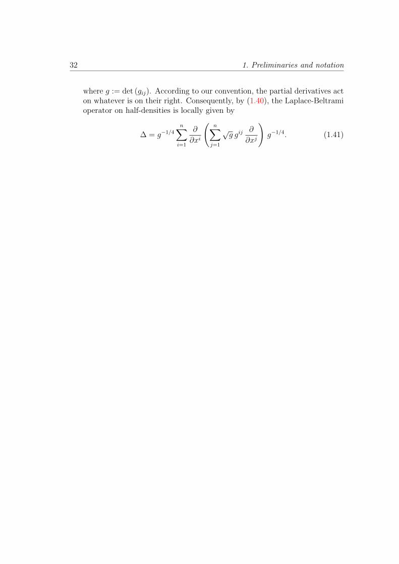
Our results concern the Laplace-Beltrami operator � on half-densities. It iswell-known from elementary di↵erential geometry that, in local coordinates,the Laplace-Beltrami operator on functions is given by
� =1pg
nX
i=1
@
@xi
nX
j=1
pg gij
@
@xj
!,
32 1. Preliminaries and notation
where g := det (gij
). According to our convention, the partial derivatives acton whatever is on their right. Consequently, by (1.40), the Laplace-Beltramioperator on half-densities is locally given by
� = g�1/4nX
i=1
@
@xi
nX
j=1
pg gij
@
@xj
!g�1/4. (1.41)

Chapter 2
Global oscillatory integrals
In the Second Chapter we will discuss how the phase function relates withHamiltonian trajectories and Lagrangian submanifolds, analysing, in partic-ular, global parametrisations with complex phase functions. In doing this,we will mainly rely on [LSV94].
Let h 2 C1(T ⇤(M)) be a Hamiltonian and let (x⇤(t; y, ⌘), ⇠⇤(t; y, ⌘)) bethe Hamiltonian trajectories generated by h. We call Lagrangian submaiofoldgenerated by h the submanifold of T ⇤R⇥ (T ⇤M \ {0})⇥ (T ⇤M \ {0}) definedby:
⇤h
:= {((t, ⌧), (x, ⇠), (y,�⌘)) | ⌧ = �h(y, ⌘), x = x⇤(t; y, ⌘), ⇠ = ⇠⇤(t; y, ⌘)} .(2.1)
Definition 2.1. We say that a phase function ' 2 C1(R⇥M⇥(T ⇤M \{0}))parametrizes the Lagrangian manifold ⇤
h
if it can be written as
⇤h
= {((t,'t
(t, x⇤; y, ⌘)), (x⇤,'x
(t, x⇤; y, ⌘)), (y,'y
(t, x⇤; y, ⌘)))}
for (t, x⇤; y, ⌘) 2 C'
(see Def. (1.6)), where we dropped the argument (t; y, ⌘)of x⇤ for notational convenience.
From this point on, we allow our phase functions to be complex-value, with=' non-negative and =' > 0 outside a small neighbourhood of x⇤(t; y, ⌘). Itis well-established that, in general, it is not possible to globally parametrizea Lagrangian manifold with a real phase function, due to some obstructionsmotivated by the presence of caustics. Laptev, Safarov and Vassiliev [LSV94]proved that the adoption of a complex phase function circumvents the prob-lem and allows one to answer positively the question of the existence of aglobal parametrization.
33

34 2. Global oscillatory integrals
2.1 The phase function revisited
Definition 2.2. Given a Hamiltonian h, we say that a complex phase func-tion ' 2 C1(R ⇥M ⇥ (T ⇤M \ {0})) is of class F
h
if it fulfils the followingadditional conditions:
'(t, x⇤(t; y, ⌘); y, ⌘) = 0; (2.2a)
gradx
'(t, x; y, ⌘)|x=x
⇤(t;y,⌘) = ⇠⇤(t; y, ⌘); (2.2b)
det @x
↵@⌘
�
'(t, x; y, ⌘)��x=x
⇤(t;y,⌘)6= 0. (2.2c)
The condition (2.2c) is called non-degeneracy condition.
The set Fh
is actually non empty and connected. Before proving thisclaim, we state and prove the main property of elements in F
h
that justifiesits introduction.
Theorem 2.3. Let ' 2 Fh
. Then ' globally parametrizes ⇤h
.
Proof. Di↵erentiating (2.2a) with respect to t, we obtain:
@t
'(t, x⇤(t; y, ⌘); y, ⌘) + @x
↵'(t, x⇤(t; y, ⌘); y, ⌘) x⇤↵(t; y, ⌘) = 0
Since by (1.31) x⇤↵(t; y, ⌘) = @⇠
↵
h(y, ⇠), the Euler identity (1.33) yields:
@t
'(t, x⇤(t; y, ⌘); y, ⌘) = �h(y, ⌘). (2.3)
Di↵erentiating (2.2a) with respect to y gives:
@x
↵'(t, x⇤(t; y, ⌘); y, ⌘) @y
x⇤↵(t; y, ⌘) + @y
'(t, x⇤(t; y, ⌘); y, ⌘) = 0.
Using (2.2b) and the fact that the Hamiltonian flow preserves the canonical1�form, we get:
⇠⇤↵
(t; y, ⌘) @y
x⇤↵(t; y, ⌘) + @y
'(t, x⇤(t; y, ⌘); y, ⌘)
=⌘ + @y
'(t, x⇤(t; y, ⌘); y, ⌘) = 0,
from which@y
'(t, x⇤(t; y, ⌘); y, ⌘) = �⌘. (2.4)
In view of (2.2b), (2.3) and (2.4) we arrive at the required result.
Remark 2.4. Observe that the constraint (2.2c) is not redundand, as longas global parametrization is concerned. In fact, we resorted to the non-degeneracy condition in disguise throughout the above proof; it guaranteesthat @
⌘
'(t, x; y, ⌘) = 0 has as unique global solution x = x⇤(t; y, ⌘), makingeverything well-defined.

2.1 The phase function revisited 35
Proposition 2.5. The set Fh
is non empty.
Proof. We will provide a constructive proof, exhibiting a distinguished classof phase functions in F
h
. Let b 2 C1(R⇥M ⇥ T ⇤M) be a positively homo-geneous function of degree 1 in ⌘ satisfying the following conditions:
(a) b(t, x; y, ⌘) = O(kx� x⇤k2k⌘k) in a small neighbourhood of x⇤;
(b) =h@2x
b(t, x; y, ⌘)|x=x
⇤(t;y,⌘)
i> 0;
(c) = b(t, x; y, ⌘) > 0 for x 6= x⇤(t; y, ⌘).
For every x, y,2 M , let �yx
: [0, 1] ! M be the shortest geodesic connectiongx to y, such that �y
x
(0) = x and �yx
(1) = y. We claim that the phase function
'(t, x; y, ⌘) = h⇠⇤(t; y, ⌘) , �xx
⇤(0)i+ b(t, x; y, ⌘) (2.5)
satisfies (2.2a)�(2.2c).Indeed, in any coordinate system, we can expand ' in Taylor series about
x = x⇤(t; y, ⌘):
'(t, x; y, ⌘) = (x�x⇤)↵⇠↵
+1
2@2x
↵
x
�
'��x=x
⇤ (x�x⇤)↵(x�x⇤)�+o(kx�x⇤k2 k⌘k).(2.6)
We see that (2.2a) and (2.2b) hold. We only need to show that (2.2c) holds.By direct inspection of (2.6), we have:
< @x
↵@⌘
�
'��x=x
⇤ = @⌘
�
⇠⇤↵
�< @2x
↵
x
�
'��x=x
⇤ @⌘�
x⇤ �,
= @x
↵@⌘
�
'��x=x
⇤ = �= @2x
↵
x
�
'��x=x
⇤ @⌘�
x⇤ � = �= @2x
↵
x
�
b��x=x
⇤ @⌘�
x⇤ �.
Introducing the notation
Z↵�
:= < @x
↵
⌘
�
'��x=x
⇤ + i= @x
↵
⌘
�
'��x=x
⇤ ,
and resorting to (1.36), we get
Z⇢↵
= (@2x
⇢
x
�
'��x=x
⇤)�1 Z
��
= < @x
⇢
⌘
↵
'|x=x
⇤ = (@2x
⇢
x
�
'��x=x
⇤)�1 < @
x
�
⌘
�
'��x=x
⇤
+ = @x
⇢
⌘
↵
'|x=x
⇤ = (@2x
⇢
x
�
'��x=x
⇤)�1 = @
x
�
⌘
�
'��x=x
⇤
(2.7)
Now, the matrix on the right-hand side is positive definite; if we can showthat its determinant is non-vanishing, then we will get the required result viaBinet’s Theorem. Let us prove that its kernel contains only the zero vector.Plugging in the definition of all of the objects involved, it is easy to see that

36 2. Global oscillatory integrals
⇥< @
x
⇢
⌘
↵
'|x=x
⇤ = (@2x
⇢
x
�
'��x=x
⇤)�1 < @
x
�
⌘
�
'��x=x
⇤
+= @x
⇢
⌘
↵
'|x=x
⇤ = (@2x
⇢
x
�
'��x=x
⇤)�1 = @
x
�
⌘
�
'��x=x
⇤
⇤v� = 0 (2.8)
if and only ifh@
⌘
x⇤ , v i = 0 ^ h @⌘
⇠⇤ , v i = 0.
As the canonical transformation is non-degenerate, then v = 0.
Chapter 3
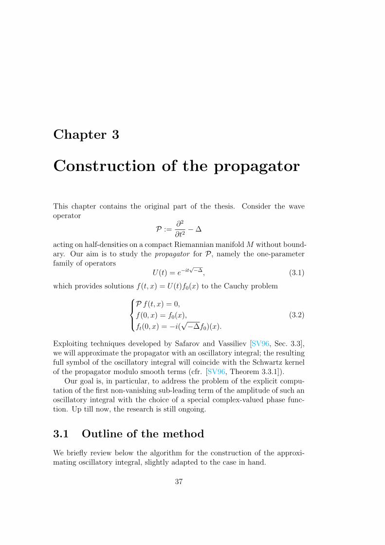
Construction of the propagator
This chapter contains the original part of the thesis. Consider the waveoperator
P :=@2
@t2��
acting on half-densities on a compact Riemannian manifoldM without bound-ary. Our aim is to study the propagator for P , namely the one-parameterfamily of operators
U(t) = e�it
p��, (3.1)
which provides solutions f(t, x) = U(t)f0(x) to the Cauchy problem
8><
>:
P f(t, x) = 0,
f(0, x) = f0(x),
ft
(0, x) = �i(p��f0)(x).
(3.2)
Exploiting techniques developed by Safarov and Vassiliev [SV96, Sec. 3.3],we will approximate the propagator with an oscillatory integral; the resultingfull symbol of the oscillatory integral will coincide with the Schwartz kernelof the propagator modulo smooth terms (cfr. [SV96, Theorem 3.3.1]).
Our goal is, in particular, to address the problem of the explicit compu-tation of the first non-vanishing sub-leading term of the amplitude of such anoscillatory integral with the choice of a special complex-valued phase func-tion. Up till now, the research is still ongoing.
3.1 Outline of the method
We briefly review below the algorithm for the construction of the approxi-mating oscillatory integral, slightly adapted to the case in hand.
37

38 3. Construction of the propagator
Step One Start with the oscillatory integral:
U(t) =1
(2⇡)n
Zei'(✏;t,x;y,⌘) · 1 · µ(t, x; y, ⌘) d
'
(✏; t, x; y, ⌘) d⌘, (3.3)
where:
• The phase function ' : [0,+1)⇥R⇥M ⇥ (T ⇤M \ {0}) ! C is chosento be
'(✏; t, x; y, ⌘) =
Zx
x
⇤⇣ dz +
i✏h(y, ⌘)
2[dist(x⇤, x)]2 . (3.4)
In the above equation, the path of integration is the shortest geodesicfrom x⇤(t; y, ⌘) to x and ⇣ is the result of parallel transport of ⇠⇤(t; y, ⌘)along this path. Furthermore, dist denotes the Riemann geodesic dis-tance, h(y, ⌘) is the Hamiltonian and ✏ a positive parameter. Observethat ' is of class F
h
.
• It is well-known in the subject literature that the principal symbol ofthe operator P is 1. This justifies our initial choice for the amplitude ofthe oscillatory integral. At a later stage, we will compute a correction.
• The function µ : R⇥M ⇥ (T ⇤M \ {0}) is a smooth cut-o↵ such that
(i) µ(t, x; y, ⌘) = 0 on {(t, x; y, ⌘) | |h(y, ⌘)| 1/2};(ii) µ(t, x; t, ⌘) = 1 on the intersection of {(t, x; y, ⌘) | |h(y, ⌘)| � 1}
with some conical neighbourhood of {(t, x⇤(t; t, ⌘); y, ⌘)};(iii) µ(t, x; y,↵⌘) = µ(t, x; y, ⌘) for ↵ � 1 on {(t, x; y, ⌘) | |h(y, ⌘)| � 1}.
In what follows, we will neglect the cut-o↵ µ, setting it to 1 in ourcalculations. This can safely be done because we will always workunder the assumption that x lies in a geodesic neighbourhood of x⇤
small enough.
• d'
: [0,+1)⇥ R⇥M ⇥ (T ⇤M \ {0}) ! C is defined by:
d'
(✏; t, x; y, ⌘) =⇥det2
�'x
↵
⌘
�
�⇤1/4. (3.5)
It is easy to see that d'
behaves as a half-density in x and as the inverseof a half-density in y. Its presence is required to guarantee that the fullsymbol is a scalar and that the principal symbol is independent of thechoice of the phase function.

3.1 Outline of the method 39
Step Two Let the wave operator P act on U(t); we obtain a new oscillatoryintegral with amplitude
a(✏; t, x; y, ⌘) = e�i'(✏;t,x;y,⌘) (d'
(✏; t, x; y, ⌘))�1 P�ei'(✏;t,x;y,⌘) d
'
(✏; t, x; y, ⌘)�.
(3.6)The amplitude a can be decomposed as
a(✏; t, x; y, ⌘) = a2(✏; t, x; y, ⌘) + a1(✏; t, x; y, ⌘) + a0(✏; t, x; y, ⌘),
where the subscripts in the right-hand side refer to the degree of homogeneityin ⌘.
Step Three Exclude the dependence of a on x. This procedure is calledreduction of the amplitude. It can be done by means of special operatorslocally defined as follows (cfr. [CDV13, Sec. 2], [SV96] for further details).Let
�↵
� := [('x
µ
⌘
⌫
(✏; t, x; y, ⌘))�1]↵
�
and introduce the first-order linear partial di↵erential operators given by
L↵
:= �↵
�
@
@x�
, ↵ = 1, . . . , n := dimM. (3.7)
Subsequently, by combining these operators and di↵erentiation with respectto ⌘, define:
B�1,r := i(d'
)�1 @
@⌘�
d'
0
@1 +X
1|↵|2r�1
(�'⌘
)↵
↵!(|↵|+ 1)L↵
1
A L�
. (3.8)
Lastly, define:
S�r
:=
(( · )|
x=x
⇤ r = 0,
S0 (B�1,r)r r 2 Z
>0.(3.9)
Let a = a2 + a1 + a0 + . . . be the reduced amplitude, called (full) symbolof the oscillatory integral, where, as usual, the subscripts label the degreeof homogeneity in ⌘. The homogeneous components are obtained by thefollowing formulae:
a2 = S0 a2, (3.10)
a1 = S�1 a2 +S0 a1, (3.11)
a0 = S�2 a2 +S�1 a1 +S0 a0, (3.12)
. . . (3.13)
40 3. Construction of the propagator
The procedure for excluding the x-dependence acts, albeit in disguise, as amultiple integration by parts. We will show this fact in our first example.
Step Four The amplitude of the oscillatory integral approximating U(t) isobtained by adding an unknown correction independent of x to the originalamplitude:
1 + f�1(t; y, ⌘) + f�2(t; y, ⌘) + . . . ,
subsequently determined by solving the transport equations, degree of ho-mogeneity by degree of homogeneity, with appropriate initial conditions att = 0. In particular, f�1(0; y, ⌘) = 0. Step Four can be avoided by adoptinga general amplitude directly in Step One, instead of carrying out the compu-tation with amplitude 1 beforehand. Nonetheless, although slightly longer,our strategy has the advantage of making calculations easier.
3.2 Solution for small times
Before tackling the problem in a general fashion, in order to get a betterfeeling of how the method works, we will discuss the case in which the timeparameter t is small. Under such an assumption, we can drop the imaginarypart of the phase function and work with a real-valued, linear phase function.In fact, if t is su�ciently small, we are guaranteed that the geodesics do notcross. In particular, we will show that the above procedure adds up, for theleading term, to a result that matches what we would obtain through heatkernel methods.
Consider the real-valued phase function
'(0; t, x; y, ⌘) =
Zx
x
⇤⇣ dz. (3.14)
See paragraph below formula (3.4) for a precise definition. In geodesic normalcoordinates centred at x⇤(t; y, ⌘), the phase function has a particularly simpleexpression:
'(0; t, x; y, ⌘) = (x� x⇤(t; y, ⌘))↵ ⇠⇤↵
(t; y, ⌘).
The amplitude can be written as
a(t, x; y, ⌘) = (d'
)�1 e�i'(t,x;y,⌘)
@2
@t2��
�ei'(t,x;y,⌘) d
'
.
From now on in this section, unless otherwise stated, arguments (t; y, ⌘) for⇠⇤ and x⇤ and (t, x; y, ⌘) for ' will be understood. Furthermore, Riemann

3.2 Solution for small times 41
tensors, Ricci tensors and Ricci scalars are always assumed to be evaluated atx⇤. Singling out its component positively homogeneous in ⌘, the amplitudewill read
a(t, x; y, ⌘) = a2(t, x; y, ⌘) + a1(t, x; y, ⌘) + a0(t, x; y, ⌘),
where, resorting to the decomposition (A.8), we have
a2(t, x; y, ⌘) = �('t
)2 + Aµ⌫ 'x
µ 'x
⌫ ,
a1(t, x; y, ⌘) = i['tt
+ 2't
(ln d'
)t
� Aµ⌫'x
µ
x
⌫ � 2Aµ⌫ 'x
µ (ln d'
)x
⌫ � Bµ 'x
µ ],
a0(t, x; y, ⌘) = d�1'
[(d'
)tt
� Aµ⌫ (d'
)x
µ
x
⌫ ]� Bµ(ln d'
)x
⌫ � C.
The subscript denotes the degree of positive homogeneity in ⌘. We stressonce again that a2, a1 and a0 are scalars.
Detailed calculations that will be provided in a separate paper, relyingon Taylor expansions about t = 0 and integration by parts, lead us to thefollowing result.
Proposition 3.1. The reduced amplitude a0(t; y, ⌘) at the leading order isgiven by:
a0(t; y, ⌘) = �1
6R(y) +O(t). (3.15)
In particular,
(a) S�2 a2(t; y, ⌘) =13R(y) +O(t),
(b) S�1 a1(t; y, ⌘) = �13R(y) +O(t),
(c) S0 a0(t; y, ⌘) = �16R(y) +O(t),
where the operators S�r
are defined in accordance with (3.9).
We now look for a correction to the symbol of the propagator of the form
1 + f�1(t; y, ⌘).
In view of the above discussion, the transport equation reads
�2i h(y, ⌘)df�1
dt(t; y, ⌘)� 1
6R(y) +O(t) = 0,
with initial conditionf�1(0; y, ⌘) = 0.
42 3. Construction of the propagator
The solution is given by
f�1(t; y, ⌘) =i
12h(y, ⌘)R(y) t+O(t2).
We arrive in the end at a formula for the sought amplitude
A(t; y, ⌘) = 1 +i
12h(y, ⌘)R(y) t+O(t2). (3.16)
It can be shown that the Weyl coe�cients computed out of (3.16) and theWeyl coe�cients obtained through heat kernel methods coincide. We referthe reader to Appendix B for further details and calculations.
3.3 The complex-valued phase function
The previous example shows how the construction goes through in the simpli-fied case of real-valued phase function. As soon as we move to a more generalsetting, considering the complex-valued phase function (3.4) in its entirety,non-trivial computational issues arise, calling for deeper analysis and under-standing. In this section, we will investigate the property of the Levi-Civitaphase function (3.4) in an arbitrary coordinate system. Subsequently, wewill apply our analysis to the case where M is a 2�sphere equipped with thestandard metric.
One of the advantages of (3.4) is that it is written in coordinate-free form,making it very versatile. Nonetheless, when carrying out computations, weneed an explicit local representation for ' in some coordinate patch. Tobegin with, let us concentrate on the real part of ':
'(0; t, x; y, ⌘) =
Zx
x
⇤⇣ dz.
Let �xx
⇤ : [0, 1] ! M be the (unique) shortest geodesic connecting x⇤ tox. The uniqueness is guaranteed by taking x in a geodesic neighbourhoodof x⇤. Let r denote the Levi-Civita connection on the tangent bundle TM .With slight abuse of notation, we denote by the same symbol the inducedconnection on the cotangent bundle T ⇤M . We have
'(t, x; y, ⌘) =
Zx
x
⇤⇣ dz =
Z 1
0
hP [�xx
⇤ , s] ⇠⇤(t; y, ⌘) , �xx
⇤(s)i ds
=
Z 1
0
h ⇠⇤(t; y, ⌘) , �xx
⇤(0) i ds
= h ⇠⇤(t; y, ⌘) , �xx
⇤(0) i,
(3.17)

3.3 The complex-valued phase function 43
where P [�xx
⇤ , s] : T ⇤Mx
⇤ ! T ⇤M�
x
x
⇤ (s) denotes the parallel transport alongthe geodesic �x
x⇤ . h · , · i denotes the (point-wise) canonical pairing betweentangent and cotangent space. We observe that the scalar function
hP [�xx
⇤ , s] ⇠⇤(t; y, ⌘) , �xx
⇤(s)i
is actually independent of s. In fact, as the Levi-Civita connection is metric-compatible, we have
d
dshP [�x
x
⇤ , s] ⇠⇤(t; y, ⌘) , �xx
⇤(s)i =hr⇤�
x
x
⇤ (s)P [�x
x
⇤ , s] ⇠⇤(t; y, ⌘) , �xx
⇤(s)i
+ hP [�xx
⇤ , s] ⇠⇤(t; y, ⌘) , r�
x
x
⇤ (s)�x
x
⇤(s)i=0.
(3.18)
In the last step we used the definition of parallel transport and the fact thatthe tangent vector to a geodesic is auto-parallel.
Remark 3.2. Two observations are in order:
(i) (3.17) reduces to'(t, x; y, ⌘) = (x� x⇤)↵⇠⇤
↵
(3.19)
when we choose normal geodesic coordinates. In such coordinates,�xx
⇤(s) = (x� x⇤) s and �xx
⇤(s) = �xx
⇤(0) = (x� x⇤);
(ii) From (3.17), it is clear that the Levi-Civita phase function is well-defined as long as we are not connecting two conjugate points. Formula(3.17) “feels” the path along which we are integrating, to the extentthat it depends on the initial velocity: caustics bring about ambiguity.Again, by constraining x to lie in a geodesic neighbourhood of x⇤ weput ourselves on the safe side.
Let us now include the imaginary part. With the above notation, (3.4)becomes
'(✏; t, x; y, ⌘) = h⇠⇤ , �xx
⇤(0)i+i ✏h
2
✓Z 1
0
qg↵�
(�xx
⇤(s)) �xx
⇤(0) �xx
⇤(0) ds
◆2
.
(3.20)Our aim is to obtain an expansion of (3.20) in powers of (x� x⇤). To beginwith, let us seek an approximate expression for �x
x
⇤(s). Our �xx
⇤ will be of theform
�xx
⇤(s) = x⇤ + (x� x⇤)s+ ⇢(s),
44 3. Construction of the propagator
where ⇢ is a correction term of order o(kx � x⇤k). Our ⇢ has to satisfy thegeodesic equation; this amounts to requiring:
⇢↵(s) + �↵
��
(�xx
⇤(s)) (x� x⇤)� (x� x⇤)� = 0 + o(kx� x⇤k2).
Hence:
⇢↵(s) = ��↵
��
(�xx
⇤(s)) (x� x⇤)� (x� x⇤)� + o(kx� x⇤k2).
Taking an expansion of the Christo↵el symbols in powers of (x � x⇤) andretaining the first order term only (higher orders terms are reabsorbed in theremainder), we obtain
⇢↵(s) =s(1� s)
2�↵
��
(x⇤) (x� x⇤)� (x� x⇤)�
where the coe�cient has been chosen so that the boundary conditions �xx
⇤(0) =x⇤, �x
x
⇤(1) = x are satisfied. All in all, we get:
(�xx
⇤(s))↵ = x⇤↵+s (x�x⇤)↵+s(1� s)
2�↵
��
(x⇤) (x�x⇤)� (x�x⇤)�+o(kx�x⇤k2).(3.21)
The Riemann distance function becomes
dist(x⇤, x) =
Z 1
0
qg↵�
(x⇤) (x� x⇤)↵ (x� x⇤)� ds+ o(kx� x⇤k2)
=q
g↵�
(x⇤) (x� x⇤)↵ (x� x⇤)� + o(kx� x⇤k2).(3.22)
and the phase function (3.20), in turn, reads
'(✏; t, x; y, ⌘) =(x� x⇤)↵⇠⇤↵
+1
2�↵
��
(x⇤) ⇠⇤↵
(x� x⇤)� (x� x⇤)�
+i ✏h
2g↵�
(x⇤) (x� x⇤)↵ (x� x⇤)� + o(kx� x⇤k2).(3.23)
We are now in a position to compute 'x
↵
⌘
�
��x=x
⇤ :
'x
↵
⌘
�
��x=x
⇤ = (⇠⇤⌘
�
)↵
+@
@⌘�
✓1
2�µ
↵⌫
(x⇤) ⇠⇤µ
+i ✏h
2gµ⌫
(x⇤) 2 �↵µ
◆(x� x⇤)⌫
�����x=x
⇤
= (⇠⇤⌘
�
)↵
� �µ
↵⌫
⇠⇤µ
@(x⇤)⌫
@⌘�
� i ✏hg↵⌫
(x⇤)@(x⇤)⌫
@⌘�
.
(3.24)
Remark 3.3. It is worth stressing that in the derivation of (3.23) and (3.24)we did not exploit the properties of any particular coordinate system. Theseformulae are, therefore, true in any coordinate system and we are free tochoose the most convenient one according to the peculiarities of the problemunder consideration.
3.3 The complex-valued phase function 45
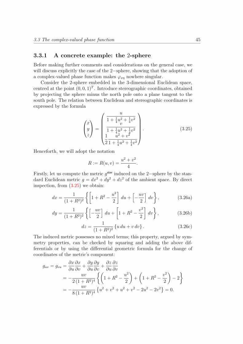
3.3.1 A concrete example: the 2-sphere
Before making further comments and considerations on the general case, wewill discuss explicitly the case of the 2�sphere, showing that the adoption ofa complex-valued phase function makes '
x⌘
nowhere singular.Consider the 2-sphere embedded in the 3-dimensional Euclidean space,
centred at the point (0, 0, 1)T . Introduce stereographic coordinates, obtainedby projecting the sphere minus the north pole onto a plane tangent to thesouth pole. The relation between Euclidean and stereographic coordinates isexpressed by the formula
0
@xyz
1
A =
0
BBBBB@
u
1 + 14u
2 + 14v
2
v
1 + 14u
2 + 14v
2
1
2
u2 + v2
1 + 14u
2 + 14v
2
1
CCCCCA. (3.25)
Henceforth, we will adopt the notation
R := R(u, v) =u2 + v2
4.
Firstly, let us compute the metric gster induced on the 2�sphere by the stan-dard Euclidean metric g = dx2 + dy2 + dz2 of the ambient space. By directinspection, from (3.25) we obtain:
dx =1
(1 +R2)2
⇢1 +R2 � u2
2
�du+
h�uv
2
idv
�, (3.26a)
dy =1
(1 +R2)2
⇢h�uv
2
idu+
1 +R2 � v2
2
�dv
�, (3.26b)
dz =1
(1 +R2)2{u du+ v dv} . (3.26c)
The induced metric possesses no mixed terms; this property, argued by sym-metry properties, can be checked by squaring and adding the above dif-ferentials or by using the di↵erential geometric formula for the change ofcoordinates of the metric’s component:
guv
= gvu
=@x
@u
@x
@v+@y
@u
@y
@v+@z
@u
@z
@v
= � uv
2 (1 +R2)4
⇢✓1 +R2 � u2
2
◆+
✓1 +R2 � v2
2
◆� 2
�
= � uv
8 (1 +R2)4�u2 + v2 + u2 + v2 � 2u2 � 2v2
= 0.
46 3. Construction of the propagator
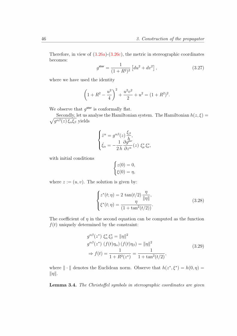
Therefore, in view of (3.26a)-(3.26c), the metric in stereographic coordinatesbecomes:
gster =1
(1 +R2)2⇥du2 + dv2
⇤, (3.27)
where we have used the identity
✓1 +R2 � u2
4
◆2
+u2v2
2+ u2 = (1 +R2)2.
We observe that gster is conformally flat.Secondly, let us analyse the Hamiltonian system. The Hamiltonian h(z, ⇠) =pg↵�(z) ⇠
↵
⇠�
yields
8><
>:
z↵ = g↵�(z)⇠�
h,
⇠↵
= � 1
2h
@gµ⌫
@z↵(z) ⇠⇤
µ
⇠⇤⌫
,
with initial conditions (z(0) = 0,
⇠(0) = ⌘,
where z := (u, v). The solution is given by:
8><
>:
z⇤(t; ⌘) = 2 tan(t/2)⌘
k⌘k ,
⇠⇤(t; ⌘) =⌘
(1 + tan2(t/2)).
(3.28)
The coe�cient of ⌘ in the second equation can be computed as the functionf(t) uniquely determined by the constraint:
g↵�(z⇤) ⇠⇤↵
⇠⇤�
= k⌘k2
g↵�(z⇤) (f(t)⌘↵
) (f(t)⌘�
) = k⌘k2
) f(t) =1
1 +R2(z⇤)=
1
1 + tan2(t/2),
(3.29)
where k · k denotes the Euclidean norm. Observe that h(z⇤, ⇠⇤) = h(0, ⌘) =k⌘k.
Lemma 3.4. The Christo↵el symbols in stereographic coordinates are given

3.3 The complex-valued phase function 47
by the formulae
�u
uu
(u, v) = � u
2(1 +R2),
�u
uv
(u, v) = �u
vu
(u, v) = � v
2(1 +R2),
�u
vv
(u, v) =u
2(1 +R2),
�v
vv
(u, v) = � v
2(1 +R2),
�v
vu
(u, v) = �v
uv
(u, v) = � u
2(1 +R2),
�v
uu
(u, v) =v
2(1 +R2).
(3.30)
Proof. As an example, we prove the formula for first Christo↵el symbol. Forthe others, the reasoning goes the same way, modulo very small adaptations.The formula for the Christo↵el symbol of the Levi-Civita connection reads
��
µ⌫
=1
2g��
✓@
@xµ
g⌫�
+@
@x⌫
gµ�
� @
@x�
gµ⌫
◆. (3.31)
Exploiting heavily the fact that the metric is diagonal, most of the termsdrop out, and we are left with
�u
uu
(u, v) =1
2guu (@
u
guu
+ @u
guu
� @u
guu
)
=1
2(1 +R2)2@
u
⇥(1 +R2)�2
⇤= �(1 +R2)�1
✓2u
4
◆
=� u
2 (1 +R2).
(3.32)
Remark 3.5. Observe that u and v label the coordinates: no summation isimplied when they appear as repeated indices.
We list below, for the sake of completeness and for later convenience, the

48 3. Construction of the propagator
expressions for the Christo↵el symbols computed at z = z⇤:
�u
uu
(u⇤, v⇤) = � tan(t/2)
1 + tan2(t/2)
⌘u
k⌘k ,
�u
uv
(u⇤, v⇤) = �u
vu
(u⇤, v⇤) = � tan(t/2)
1 + tan2(t/2)
⌘v
k⌘k ,
�u
vv
(u⇤, v⇤) =tan(t/2)
1 + tan2(t/2)
⌘u
k⌘k ,
�v
vv
(u⇤, v⇤) = � tan(t/2)
1 + tan2(t/2)
⌘v
k⌘k ,
�v
vu
(u⇤, v⇤) = �v
uv
(u⇤, v⇤) = � tan(t/2)
1 + tan2(t/2)
⌘u
k⌘k ,
�v
uu
(u⇤, v⇤) =tan(t/2)
1 + tan2(t/2)
⌘v
k⌘k .
(3.33)
u
v
•y
•x⇤
•x
Figure 3.1: Diagrammatic picture of the geometric setting in stereographiccoordinates.
Let us decompose the phase function ' = � + �✏ into real and purelyimaginary parts:
�(t, z; y, ⌘) = '(0; t, z; y, ⌘),
�✏(t, z; y, ⌘) =i ✏h
2g↵�
(z⇤) (z � z⇤)↵ (z � z⇤)� + o(kz � z⇤k2).
Equation (3.24) tells us that:
�z
↵
⌘
�
��z=z
⇤ (⇠⇤⌘
�
)↵
� �µ
↵⌫
⇠⇤µ
@(z⇤)⌫
@⌘�
, (3.34a)
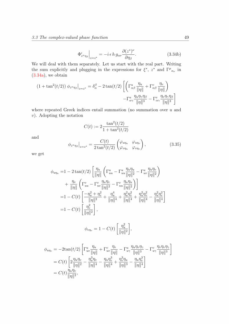
3.3 The complex-valued phase function 49
�✏
z
↵
⌘
�
���z=z
⇤= �i ✏h g
↵⌫
@(z⇤)⌫
@⌘�
. (3.34b)
We will deal with them separately. Let us start with the real part. Writingthe sum explicitly and plugging in the expressions for ⇠⇤, z⇤ and �µ
↵
⌫
in(3.34a), we obtain
(1 + tan2(t/2)) �z
↵
⌘
�
��z=z
⇤ = ��↵
� 2 tan(t/2)
✓�u
↵�
⌘u
k⌘k + �v
↵�
⌘v
k⌘k
◆
��u
↵�
⌘u
⌘�
⌘�
k⌘k3 � �v
↵�
⌘v
⌘�
⌘�
k⌘k3
�
where repeated Greek indices entail summation (no summation over u andv). Adopting the notation
C(t) := 2tan2(t/2)
1 + tan2(t/2)
and
�z
↵
⌘
�
��z=z
⇤ =C(t)
2 tan2(t/2)
✓'u⌘
u
'u⌘
v
'v⌘
u
'v⌘
v
◆, (3.35)
we get
�u⌘
u
=1� 2 tan(t/2)
⌘u
k⌘k
✓�u
uu
� �u
uu
⌘u
⌘u
k⌘k2 � �u
uv
⌘u
⌘v
k⌘k2
◆
+⌘v
k⌘k
✓�v
uu
� �v
uv
⌘u
⌘v
k⌘k2 � �v
uu
⌘u
⌘u
k⌘k2
◆�
=1� C(t)
�⌘2
u
+ ⌘2v
k⌘k2 +⌘4u
k⌘k4 +⌘2u
⌘2v
k⌘k4 +⌘2u
⌘2v
k⌘k4 � ⌘2u
⌘2v
k⌘k4
�
=1� C(t)
⌘2v
k⌘k2
�,
�v⌘
v
= 1� C(t)
⌘2u
k⌘k2
�,
�u⌘
v
= �2tan(t/2)
�u
uv
⌘u
k⌘k + �v
uv
⌘v
k⌘k � �u
u�
⌘u
⌘v
⌘�
k⌘k3 � �v
u�
⌘v
⌘v
⌘�
k⌘k3
�
= C(t)
2⌘u
⌘v
k⌘k2 � ⌘3u
⌘v
k⌘k4 � ⌘u
⌘3v
k⌘k4 +⌘3v
⌘u
k⌘k3 � ⌘u
⌘3v
k⌘k4
�
= C(t)⌘u
⌘v
k⌘k2 ,

50 3. Construction of the propagator
�v⌘
u
= C(t)⌘u
⌘v
k⌘k2 .
Summing up, we have established that
(1 + tan2(t/2)) (�z
↵
⌘
�
��z=z
⇤) = 1+ C(t)
0
BB@� ⌘2
v
k⌘k2⌘u
⌘v
k⌘k2⌘u
⌘v
k⌘k2 � ⌘2u
k⌘k2
1
CCA . (3.36)
Let us move to the purely imaginary part. Substituting (3.33) into (3.34b),one obtains
(1 + tan2(t/2))�(�✏)
z
↵
⌘
�
��z=z
⇤
�=
✓�2i✏k⌘k tan(t/2)
1 + tan2(t/2)�↵⌫
��⌫
k⌘k � ⌘⌫⌘�
k⌘k3
�◆
=
✓�2i✏
tan2(t/2)
1 + tan2(t/2)
��↵
� ⌘↵
⌘�
k⌘k2
�◆
=C(t)
0
BB@�i✏+ i✏
⌘2u
k⌘k2 i✏⌘u
⌘v
k⌘k2
i✏⌘u
⌘v
k⌘k2 �i✏+ i✏⌘2v
k⌘k2
1
CCA ,
(3.37)
where ✏ = ✏
tan(t/2) . Combining (3.36) and (3.37) we end up with
('z↵⌘�
��z=z⇤) =
1
1 + tan2(t/2)
0
BB@1 + C(t)
�i✏+ i✏
⌘2uk⌘k2 � ⌘v
k⌘k2
�C(t)
⌘u⌘vk⌘k2 (1 + i✏)
�
C(t)
⌘u⌘vk⌘k2 (1 + i✏)
�1 + C(t)
�i✏+ i✏
⌘2vk⌘k2 � ⌘u
k⌘k2
�
1
CCA
= :1
1 + tan2(t/2)M.
(3.38)
With the determinant in mind, we compute the following auxiliary products:
M11 M22 =1 + C(t)
�i✏+ i✏
⌘2u
k⌘k2 � ⌘v
k⌘k2 � i✏+ i✏⌘2v
k⌘k2 � ⌘u
k⌘k2
�
+ C(t)2�i✏+ i✏
⌘2u
k⌘k2 � ⌘v
k⌘k2
� �i✏+ i✏
⌘2v
k⌘k2 � ⌘u
k⌘k2
�
=1 + C(t) [�2i✏+ i✏� 1] + C(t)2�✏2 + ✏2
⌘2v
k⌘k2 + i✏⌘2u
k⌘k2
+✏2⌘2u
k⌘k2 � ✏2⌘2u
⌘2v
k⌘k4 � i✏⌘4u
k⌘k4 + i✏⌘2v
k⌘k2 � i✏⌘4v
k⌘k4 +⌘2u
⌘2v
k⌘k4
�
=1� C(t) (1 + i✏) + C(t)2 (1 + i✏)2⌘2u
⌘2v
k⌘k4 ,
3.4 The problem in perspective 51
M12 M21 = C(t)2 (1 + ✏)2⌘2u
⌘2v
k⌘k4 .
Hence, finally, we have a formula for the determinant:
det'z
↵
⌘
�
��x=x
⇤ =1
(1 + tan2(t/2))2(cos t� i ✏ sin t) . (3.39)
Remark 3.6. (a) The computation shows that the terms with ✏2 cancel out.In principle, it is not obvious that this should happen.
(b) Looking at (3.39), we observe that, if ✏ = 0, the determinant vanishesfor t = ⇡/2. This corresponds to the fact that the geodesics, origi-nating from the south pole, reach the equator, becoming parallel: thismimics the presence of a caustic. Here we can see how the adoptionof a complex-valued phase function allows to circumvent the singularity,making det'
z
↵
⌘
�
everywhere non-zero.
(c) We know from the general theory that d'
is a half-density in x andthe inverse of a half-density in y. The complication in the forthcomingcomputations will actually derive from d
'
. Therefore, we may pursue thestrategy of isolating the purely scalar part of d
'
factoring out a suitablepre-factor. We define:
f(✏; t, x; y, ⌘) :=det g(y)
det g(x)
�det'
x
↵
⌘
�
�2.
Recall that the determinant of the covariant metric tensor is a 2�density.We need to square the determinant of '
x
↵
⌘
�
on the right-hand side, ratherthan taking fractional powers of the determinant of the metric, becausethis makes f a proper scalar (note that '
x
↵
⌘
�
changes sign under inversionof the x- coordinates). Thus, d
'
becomes
d'
(✏; t, x; y, ⌘) =[det g(x)]1/4
[det g(y)]1/4f 1/4(✏; t, x; y, ⌘). (3.40)
Hence, for the 2-sphere we have:
f ⇤(✏; t; y, ⌘) := f(✏; t, z⇤(t; y, ⌘); y, ⌘) = (cos t� i ✏ sin t)2 . (3.41)
3.4 The problem in perspective
In this last section we will discuss the principal features of the general prob-lem, by writing full-fledged equations, pointing out the main di�culties and

52 3. Construction of the propagator
outlining possible strategies. We do not have, at the moment, a completesolution to the problem, since the research is still ongoing.
The Laplace-Beltrami operator (1.41) can be recast as follows:
� =g↵�@
@x↵
@
@x�
+⇥g�1/2
�g↵� g1/2
�x
↵
+ g1/4 g↵��g�1/4
�x
↵
⇤ @
@x�
+g�1/4�g↵� g1/2
�x
↵
�g�1/4
�x
�
+ g1/4 g↵��g�1/4
�x
↵
x
�
.
(3.42)
Hence, according to the prescriptions given in Step Two, we obtain
a2(✏; t, x; y, ⌘) = �(@t
')2 + g↵� r↵
'r�
', (3.43a)
a1(✏; t, x; y, ⌘) =i�'tt
� g↵� r↵
r�
'+ (log f 1/2)t
't
� g↵� (log f 1/2)x
↵ 'x
�
,
(3.43b)
a0(✏; t, x; y, ⌘) =(d'
)�1⇥(d
'
)tt
� g↵� r↵
r�
d'
⇤� g1/4 g↵� r
↵
r�
g�1/4,
(3.43c)
where f is the scalar function introduced in Remark 3.6. Observe that so farwe have not used the special form of our phase function: formulae (3.43a)-(3.43c) are true for a generic phase function of class F
h
. Furthermore, itemerges clearly that the components homogeneous in ⌘ of the amplitude areproper scalars. This would not be the case without the introduction of thed'
factor in the original oscillatory integral.Let us analyse the first non-trivial equation in (3.10):
a1 = S�1 a2 +S0 a1. (3.44)
Plugging (A.9) and (3.23) into (3.43a)-(3.43b) and adopting normal geodesiccoordinates, after lengthy computations we get an explicit expression fora2 and a1. Whereas S0 is nothing but the evaluation at x = x⇤, S�1 has arather complicated expression. Defining �
↵
� := ('�1x⌘
)↵
�, it is straightforwardto check that
S�1 a2 = iS0
⇢(d
'
)�1
✓@
@⌘�
d'
◆�
�
� � 1
2'⌘
k
⌘
�
�k
� (��
�)x
� + @⌘
�
��
�
�@
@x�
� 1
2'⌘
k
⌘
�
�k
� ��
�
@
@x�
@
@x�
+ ��
�
@
@⌘�
@
@x�
�a2.
(3.45)

3.4 The problem in perspective 53
In principle, all the ingredients for the computation are known. In fact, wehave
det'x⌘
=1
n!
X
{ik
},{jk
}
"i1,...,inj1,...,jn
('x⌘
)i1j1 . . . ('
x⌘
)i
n
j
n , (3.46)
and
�↵
� =(�1)↵+�
(n� 1)! det'x⌘
X
{ik
}\↵, {jk
}\�
"i1,...,in�1
j1,...,jn�1('
x⌘
)i1j1 . . . ('
x⌘
)i
n�1j
n�1 ,
(3.47)where " is the totally antisymmetric Levi-Civita symbol and ('
x⌘
)↵
� can beobtained, according to the case in hand, from (3.23) or (3.24). In practice,already at this stage, the computational di�culty is substantial. This ismainly due to the lack of compact formulae for d
'
, �↵
� and their derivatives.The various terms appearing in (3.44) are not involute from a conceptualviewpoint; rather, they are hard to handle at a practical level. For instance,(�
↵
�)x
� is given by
(�↵
�)x
� =
✓@
@x�
1
det'x⌘
◆ X
i
k
6=↵, j
k
6=�
(�1)↵+�
(n� 1)!✏i1,...,in�1
j1,...,jn�1
n�1Y
s=1
�i
s
j
s
+1
det'x⌘
X
i
k
6=↵, j
k
6=�
(�1)↵+�
(n� 1)!✏i1,...,in�1
j1,...,jn�1
n�1X
p=1
✓@
@x�
�i
p
j
p
◆Y
s 6=p
�i
s
j
s
where, to be consistent, we need to push further the expansion in powers of(x � x⇤) for '
x⌘
, up to the third order. If we resort to formula (3.24) only,in fact, we end up with incorrect and inconsistent results. As one can easilysee, things become even worse as soon as S�2 gets involved.
If we want to tackle the problem without employing computer software,we need alternative strategies. A possible way could be to try and rewriteStep Three in a more geometric way. Safarov and Vassiliev’s results do notexploit the geometric structure provided by the metric in their construction,which encompasses a high degree of generality. Some simplifications mayoccur if the Levi-Civita metric connection is taken into account.
We expect the first transport equation to give a vanishing contribution.This fact can be argued from the subprincipal symbol of the Laplace-Beltramioperator being zero. Still, understanding what actually makes it zero wouldgive a deeper insight into the general problem. All in all, seeking an ex-pression for the subleading term of the full symbol, amounts eventually tolooking for a solution to the second transport equation. This is currently thesubject of our research.

54 3. Construction of the propagator

Appendix A
Taylor expansions in normal geodesiccoordinates
In our thesis, we mainly work in normal geodesic coordinates centred atx⇤(t, x; t, ⌘), due to computational convenience. We list in this appendixsome useful formulae concerning the Taylor expansion of relevant geometricobject about x = x⇤(t, x; y, ⌘), so as to lighten the main text.
To begin with, we give a list of formulae for the metric gij
and for se-lected powers of the determinant of the metric g = det g
µ⌫
. For notationalsimplicity, we provide expansions about x = 0.
gµ⌫
=�µ⌫
+1
3R
�µ⌫⇢
x�x⇢ +1
6(r
�
R�µ⌫⇢
)x�x�x⇢
+
✓1
20(r
�
r⌧
R�µ⌫⇢
) +2
45R
�µ⇢
R �
�⌫⌧
��
◆x�x⇢x�x⌧ +O(kxk4),
(A.1)
gµ⌫ =�µ⌫ � 1
3R µ⌫
� ⇢
x�x⇢ � 1
6(r
�
R µ⌫
� ⇢
)x�x�x⇢
�✓
1
20(r
�
r⌧
R µ⌫
� ⇢
) +2
45R µ
� ⇢
R ⌫ �
� ⌧
��
+1
9R µ⌫
� ⇢
R µ⌫
� ⌧
◆x�x⇢x�x⌧
+O(kxk4),(A.2)
55
56 A. Taylor expansions in normal geodesic coordinates
g =1� 1
3R
�⇢
x�x⇢ � 1
6(r
�
R�⇢
)x�x�x⇢
�✓
1
20(r
�
r⌧
R�⇢
) +1
90R
�µ⇢
R �
�⌫⌧
��
�µ⌫ � 1
18R
�⇢
R�⌧
◆x�x⇢x�x⌧
+O(kxk4),(A.3)
g12 =1� 1
6R
�⇢
x�x⇢ � 1
12(r
�
R�⇢
)x�x�x⇢
�✓
1
40(r
�
r⌧
R�⇢
) +1
180R
�µ⇢
R �
�⌫⌧
��
�µ⌫ � 1
72R
�⇢
R�⌧
◆x�x⇢x�x⌧
+O(kxk4),(A.4)
g�12 =1 +
1
6R
�⇢
x�x⇢ +1
12(r
�
R�⇢
)x�x�x⇢
+
✓1
40(r
�
r⌧
R�⇢
) +1
180R
�µ⇢
R �
�⌫⌧
��
�µ⌫ +1
72R
�⇢
R�⌧
◆x�x⇢x�x⌧
+O(kxk4),(A.5)
g14 =1� 1
12R
�⇢
x�x⇢ � 1
24(r
�
R�⇢
)x�x�x⇢
�✓
1
80(r
�
r⌧
R�⇢
) +1
360R
�µ⇢
R �
�⌫⌧
��
�µ⌫ � 1
288R
�⇢
R�⌧
◆x�x⇢x�x⌧
+O(kxk4),(A.6)
g�14 =1 +
1
12R
�⇢
x�x⇢ +1
24(r
�
R�⇢
)x�x�x⇢
+
✓1
80(r
�
r⌧
R�⇢
) +1
360R
�µ⇢
R �
�⌫⌧
��
�µ⌫ +1
288R
�⇢
R�⌧
◆x�x⇢x�x⌧
+O(kxk4),(A.7)
All the coe�cients in the above formulae are evaluated at x = 0.

57
Plugging (A.1)-(A.7) into (1.41), we obtain, with the obvious substitutionx ! (x � x⇤), an expansion in powers of (x � x⇤) for the Laplace-Beltramioperator (1.41). From a computational perspective, it is convenient to writethe Laplacian as
� = Aµ⌫ @x
µ@x
⌫ +B⌫ @x
⌫ + C, (A.8)
and expand into Taylor series the coe�cients Aµ⌫ , B⌫ and C separately. Bydirect inspection, we get:
Aµ⌫ = �µ⌫ � 1
3R µ⌫
↵ �
(x� x⇤)↵ (x� x⇤)� +O(kx� x⇤k3), (A.9a)
B⌫ =� 1
3�µ⌫ Ric
µ�
(x� x⇤)� � 1
6[r
µ
R µ⌫
k �
+ �⌫sr
Ric�s
](x� x⇤)�(x� x⇤)
+O(kx� x⇤k3),(A.9b)
C =1
6R+
1
12[2�µ⌫r
µ
Ric⌫�
+r�
R] (x� x⇤)� +O(kx� x⇤k2). (A.9c)
58 A. Taylor expansions in normal geodesic coordinates
Appendix B
Weyl coe�cients: a comparison
The aim of this appendix is to perform a comparison between the Weyl co-e�cients computed out of (3.16) and the Weyl coe�cients predicted by heatkernel methods. We will show that they, actually, coincide.
Let �k
be the eigenvalues of the operatorp�� and let v
k
be correspond-ing orthonormal eigenfunctions. Let n � 3 be the dimension of our manifoldM . Formula (3.16) implies that the trace of the kernel of the propagator ofP is given by:
X
k
|vk
(y)|2 e�it�
k ⇡ 1
(2⇡)n
Z ✓1 +
i
12h(y, ⌘)R(y) t+O(t2)
◆e�it h(y,⌘) d⌘.
(B.1)The above formula is an approximate equality; a precise meaning can beassigned in terms of the theory of distributions. Let
N(y;�) =X
�
k
<�
|vk
(y)|2
be the local counting function. When integrated over the manifold, N(y;�)is an integer describing the number of eigenvalues smaller than �. We referthe reader to [Shu87] for a rigorous definition and detailed exposition of thespectral-theoretic objects used in this appendix.
The local counting function is useful if one wants to express, in a weaksense, the discrete sum (B.1) as an integral (again, see [Shu87]):
Z +1
0
e�it�
dN
d�(y;�) d� ' 1
(2⇡)n
Z ✓1 +
i
12h(y, ⌘)R(y) t+O(t2)
◆e�it h(y,⌘) d⌘.
(B.2)
59

60 B. Weyl coe�cients: a comparison
In light of well-known results from the literature (cfr. [Min53,MP49, Ivr98,Ros97]), we put:
N(y;�) = a(y)�n + b(y)�n�1 + c(y)�n�2 + . . . , �! +1. (B.3)
The coe�cients in the above expansion are called Weyl coe�cients.We can put forward a similar analysis for the trace of the heat kernel,
which has been very well studied over the years. In particular, it admits thefollowing expansion for t ! 0+:
Z +1
0
e�t�
2 dN
d�(y;�) d� =
1
(4⇡t)n/2
✓1 +
1
6R(y) t+O(t2)
◆ pdet g(y).
(B.4)A comparison between (B.4) and (B.2) is made possible by plugging (B.3) inthe integral in the left-hand side and collating the resulting Weyl coe�cients.
Fact B.1. The first three Weyl coe�cients computed from (B.4) are:
ah
(y) =1
4n
2
2
n�(n2 ) ⇡n
2,
bh
(y) = 0,
ch
(y) =1
4n
2
R(y)
6�(n2 ) ⇡n
2.
Here the subscript h emphasises the fact that these Weyl coe�cients havebeen computed on the basis of (B.4).
Proof.
Z +1
0
e�t�
2 �na(y)�n�1 + (n� 1)b(y)�n�2 + (n� 2)c(y)�n�3
�d� =
=n a(y)
Z +1
0
e�t�
2�n�1 d�+ (n� 1) b(y)
Z +1
0
e�t�
2�n�2 d�
+ (n� 2) c(y)
Z +1
0
e�t�
2�n�3 d�
=n a(y)
tn
2
Z 1
0
e�z
2zn�1 dz +
(n� 1) b(y)
tn
2�12
Z 1
0
e�z
2zn�2 dz
+(n� 2) c(y)
tn
2�1
Z 1
0
e�z
2zn�3 dz
=a(y)
n�(n2 )
2tn
2
�+ b(y)
(n� 1)�(n�1
2 )
2tn
2�12
�+ c(y)
�(n2 )
tn
2�1
�.

61
In the last step we made use of the known resultZ 1
0
e�z
2zn�1 dz =
�(n2 )
2,
and of the following property of the Gamma function:
�(z + 1) = z�(z) ) �⇣n2� 1
⌘=
�(n2 )
(n2 � 1)=
2�(n2 )
(n� 2).
Equating the coe�cients of the same powers of t on the two sides of (B.4),we get:
a(y)
n�(n2 )
2tn
2
�=
1
(4⇡)n
2 tn
2,
b(y)
(n� 1)�(n�1
2 )
2tn
2�12
�= 0,
c(y)
�(n2 )
tn
2�1
�=
R(y)
6 (4⇡)n
2 tn
2�1,
from which the clam ensues.
Fact B.2. The first three Weyl coe�cients computed from (B.2) are:
a(y) =1
2n2
n�(n2 ) ⇡n
2,
b(y) = 0,
c(y) =1
2nR(y)
6�(n2 ) ⇡n
2.
Proof. After the substitution, the left-hand side in (B.2) readsZ 1
0
⇥n a(y) ⇢n�1 + (n� 1) b(y) ⇢n�2 + (n� 2) c(y) ⇢n�3
⇤e�it⇢ d⇢.
As far as the right-hand side is concerned, after observing that in our co-ordinate system h(y, ⌘) =
p⌘21 + . . .+ ⌘2
n
= |⌘|, we can switch to (hyper-)spherical coordinates for ⌘ and write:
1
(2⇡)n
Z ✓1 +
i
12h(y, ⌘)R(y) t
◆e�it h(y,⌘) d⌘
=1
(2⇡)n2⇡
n
2
�(n2 )
Z 1
0
✓1 +
itR(y)
12⇢
◆e�it⇢ ⇢n�1 d⇢
=1
2n2
⇡n
2�(n2 )
Z 1
0
✓⇢n�1 +
itR(y)
12⇢n�2
◆e�it⇢ d⇢
=1
2n2
⇡n
2�(n2 )
Z 1
0
✓⇢n�1 + (n� 2)
R(y)
12⇢n�3
◆e�it⇢ d⇢,
62 B. Weyl coe�cients: a comparison
where in the last passage we got rid of the factor it by performing integrationby parts. Reading o↵ the coe�cients yields the desired result.
All in all, we have established that ah
(y) = a(y), bh
(y) = b(y) and ch
(y) =c(y).
Appendix C
An insight into amplitude reduc-tion
In this appendix we show that the procedure for the amplitude reductionoutlined in Section 3.1 gives the same result as the integration by parts inthe case of small time parameter t.
When t ! 0, (3.7) and (3.8) become:
L↵
' ��↵
@
@x�
=@
@x↵
, (C.1)
B�1,r ' i@
@⌘�
0
@1 +X
1|↵|2r�1
(�'⌘
)↵
↵!(|↵|+ 1)
@
@x↵
1
A @
@x�
. (C.2)
Since
'⌘
�
' @
@⌘�
[(x� y)↵ ⌘↵
] = (x� y)�,
we have:
S0 B�1,1 = i@
@⌘�
@
@x�
,
from which we get
S�1 a1 ' i@
@⌘�
@
@x�
i
3�µ⌫ Ric
µ↵
⌘⌫
(x� y)↵�
= �1
3�µ⌫ Ric
µ↵
��⌫
�↵�
= �1
3R.
(C.3)
63
64 C. An insight into amplitude reduction
As far as the case r = 2 is concerned in (C.2), we observe that, upon eval-uation against S0, the only non-vanishing contribution to the sum on theright-hand side comes from |↵| = 1. Namely,
B�1,2 = B�1,1 +O(|x� y|).
Therefore
S�2 = S0 (B�1,2)2 = � @
@⌘�
@
@x�
@
@⌘�
@
@x�
.
We conclude that the contribution to the symbol coming from the termpositively homogeneous in ⌘ of degree 2 is given by
S�2 a2 ' � @
@⌘�
@
@x�
@
@⌘�
@
@x�
�1
3R µ⌫
↵ ⇢
⌘µ
⌘⌫
(x� y)↵ (x� y)⇢�
=1
3R.
(C.4)
Formulae (C.3) and (C.4) coincide respectively with (b) and (a) in Propo-sition 3.1.

Bibliography
[CDV13] O. Chervova, R. Downes, and D. Vassiliev, The spectral function of a first orderelliptic system, Journal of Spectral Theory 3 (2013), 317–360.
[GS94] A. Grigis and J. Sjostrand, Microlocal analysis for di↵erential operators: Anintroduction, Cambridge University Press, 1994.
[Hor83] L. Hormander, The analysis of linear partial di↵erential operators I: Distributiontheory and fourier analysis, Springer-Verlag, 1983.
[Hor85] , The analysis of linear partial di↵erential operators III: Pseudo-di↵erential operators, Springer-Verlag, 1985.
[Ivr98] V. Ivrii, Microlocal analysis and precise spectral asymptotics, Springer, 1998.
[LSV94] A. Laptev, Yu. Safarov, and D. Vassiliev, On global representation of lagrangiandistributions and solutions of hyperbolic equations, Communications on Pure andApplied Mathematics 47 (1994), no. 11.
[Min53] S. Minakshisundaram, Eigenfunctions on Riemannian manifolds, Journal of In-dian Mathematical Society 17 (1953), 158–165.
[MP49] S. Minakshisundaram and A. Pleijiel, Some properties of the eigenfunctions ofthe Laplace-operator on Riemannian manifolds, Canadian Journal of Mathemat-ics 1 (1949), 242–256.
[Ros97] S. Rosenberg, The Laplacian on a Riemannian manifold, Cambridge UniversityPress, 1997.
[Shu87] M. A. Shubin, Pseudodi↵erential operators and spectral thery, Springer-Verlag,1987.
[SV96] Yu. Safarov and D. Vassiliev, The asymptotic distribution of eigenvalues of par-tial di↵erential operators, American Mathematical Society, 1996.
65