ATMOSPHERIC OPTICS GROUP January 2010

Scientific Report on Whole Sky Imager Characterization

Of Sky Obscuration by Clouds For the Starfire Optical Range

Scientific Report for AFRL Contract

Contract FA9451-008-C-0226

Janet E. Shields Monette E. Karr

Art R. Burden Vincent W. Mikuls

Jacob R. Streeter Richard W. Johnson William S. Hodgkiss

Justin G. Baker

UNIVERSITY OF

CALIFORNIA SAN DIEGO

SCRIPPS INSTITUTION

OF OCEANOGRAPHY MARINE PHYSICAL LAB San Diego, CA 92152-6400

Standard Form 298 (Rev. 8/98)

REPORT DOCUMENTATION PAGE

Prescribed by ANSI Std. Z39.18

Form Approved OMB No. 0704-0188

The public reporting burden for this collection of information is estimated to average 1 hour per response, including the time for reviewing instructions, searching existing data sources, gathering and maintaining the data needed, and completing and reviewing the collection of information. Send comments regarding this burden estimate or any other aspect of this collection of information, including suggestions for reducing the burden, to Department of Defense, Washington Headquarters Services, Directorate for Information Operations and Reports (0704-0188), 1215 Jefferson Davis Highway, Suite 1204, Arlington, VA 22202-4302. Respondents should be aware that notwithstanding any other provision of law, no person shall be subject to any penalty for failing to comply with a collection of information if it does not display a currently valid OMB control number. PLEASE DO NOT RETURN YOUR FORM TO THE ABOVE ADDRESS. 1. REPORT DATE (DD-MM-YYYY) 2. REPORT TYPE 3. DATES COVERED (From - To)

4. TITLE AND SUBTITLE 5a. CONTRACT NUMBER

5b. GRANT NUMBER

5c. PROGRAM ELEMENT NUMBER

5d. PROJECT NUMBER

5e. TASK NUMBER

5f. WORK UNIT NUMBER

6. AUTHOR(S)

7. PERFORMING ORGANIZATION NAME(S) AND ADDRESS(ES) 8. PERFORMING ORGANIZATION REPORT NUMBER

9. SPONSORING/MONITORING AGENCY NAME(S) AND ADDRESS(ES) 10. SPONSOR/MONITOR'S ACRONYM(S)

11. SPONSOR/MONITOR'S REPORT NUMBER(S)

12. DISTRIBUTION/AVAILABILITY STATEMENT

13. SUPPLEMENTARY NOTES

14. ABSTRACT

15. SUBJECT TERMS

16. SECURITY CLASSIFICATION OF: a. REPORT b. ABSTRACT c. THIS PAGE

17. LIMITATION OF ABSTRACT

18. NUMBER OF PAGES

19a. NAME OF RESPONSIBLE PERSON

19b. TELEPHONE NUMBER (Include area code)

01/31/10 Final Report 2/1/08-10/1/09

Scientific Report on the Whole Sky Imager Characterization of Sky Obscuration by Clouds for the Starfire Optical Range

FA9451-008-C-0226

Shields, Janet E. Karr, Monette E. Burden, Art B. Mikuls, Vincent W. Streeter, Jacob R. Johnson, Richard W. Hodgkiss, William S.

Marine Physical Laboratory of the Scripps Institution of Oceanography University of California, San Diego 291 Rosecrans Street San Diego, California 92106

AF Research Laboratory (DET 8) 2251 Maxwell Street, SE KIRTLAND AFB, NM 87117-5773 Attn: Kyle Dufaud, kyle.dufaud@afmc.af.smil.mil

AFRL/RDKL

Distribution unlimited; per contract conditions, the data and reports generated from this project are deemed unclassified with unlimited distribution, while the meetings with USAF representatives and contractors that took place as part of the project were deemed classified, they have been excluded from the contents of this report.

This report summarizes work conducted for the Airforce Research Lab (AFRL) at Kirtland Airforce base on contract FA9451-008-C-0226 by the Atmospheric Optics Group of the Marine Physical Laboratory at the Scripps Institution of Oceanography, UC San Diego. The primary goal of this project was to gather a multi-site data base of cloud distribution over the whole sky, in order to study the effect of sky obscuration by clouds. There are numerous applications that require looking either up or down through the cloud deck, including satellite tracking, detecting ground targets from the air, and so on. For many of these applications, it would be useful to have a large high quality data base with which we could study questions such as: how often do clouds block the line of sight; how persistent is the blockage; how well do models based on satellite imagery truly represent the impact of clouds; how often does the satellite imagery detect small or very thin clouds and what is their impact; and so on.

Whole Sky Imager, Clouds, Sky, Obscuration

Unclassified Unclassified Unclassified None 98

Anne J. Footer

858-534-1802

Reset

COORDINATION RECORD FOR SECURITY & POLICY REVIEW

377th Air Base Wing

Office of Public Affairs

Release #: 377ABW-2011-1183

OPS #: OPS-11-1571

Request public release clearance for:

Title:

Author(s):

Name of publication, symposium, or conference:

Date to be presented/published:

Location:

Requestor's suspense date:

7/1/2011

Is another organization funding/involved with this program?

Is coordination required?

Funding Level:

If applicable, provide PA case # of previously cleared document(s):

Higher Headquarters review is required for material concerning national interests, foreign policy, DOD or U.S. Government policy, subjects of potential controversy among DOD components or with other federal agencies, or the degree of success of intelligence efforts.Additionally, review is required for the following subject areas: New weapons, weapon systems, or significant modification or improvements to existing weapons or system, equipment, or techniques, and use of weapons on the battlefield, as well as presentations conducted at NATO conferences.

Name Office Symbol Phone Email

Shields, Janet University of California, San Diego

505-846-4646 jshields@ucsd.edu

Name Office Symbol Phone Email

Dufaud, Kyle RDSOT 246-4646 Kyle.Dufaud@kirtland.af.mil

Paper

Whole Sky Imager CharacterizationOf Sky Obscuration by CloudsFor the Starfire Optical Range

Whole Sky Imager Characterization of Sky Obscuration by Clouds

AFRL/RDS

01/11/2010

No

Yes

6.1x 6.2o 6.3o 6.4o 6.5o SBIRo Othero N/Ao

If yes, name of organization:

PA #

Certification

The security classification guide for this technology/program has been reviewed.

N/A

x

x

o

Name Status Review Date Comments

Kyle Dufaud, RDSO, 246-4646 Open 6/3/2011 10:49:00 AM

Kyle Dufaud, RDSO, 246-4646 Submitted 7/20/2011 9:09:00 AM

Kyle Dufaud, RDSO, 246-4646 Program Manager Approved 7/20/2011 9:11:00 AM

Dennis Montera, RDSAM, 246-5130 Technical OPSEC Approved 7/21/2011 10:33:00 AM

Charles Matson, RDS, 246-2049 Technical Advisor Approved 7/21/2011 3:57:00 PM

Lori Everitt, RDSO, 246-4050 Branch Approved 7/25/2011 12:50:00 PM

Kent Wood, RDS, 246-6783 Division Approved 7/25/2011 2:30:00 PM

Iris Puentes, RDOS, 246-4710 Program OPSEC Approved 7/25/2011 3:36:00 PM

Michael Kleiman, 377 ABW/PA, 246-4704

Public Affairs Approved 8/11/2011 10:27:00 AM

Approved for public release on 11 Aug 11.

The material has been reviewed for sensitivities associated with ITAR (export control) regulations, Commerce Control List (CCL), USML (U.S. Munitions List), MCTL (Military Critical Technology List).

This document is accurate, technically correct, unclassified, does not violate proprietary rights, and does not contain information from limited distribution documents.

This document does not reveal enough detailed information that will help enable an adversary/competitor to duplicate/apply/deny/counter the technology, in accordance with AFI 10-1101.

Does this material contain technology or information listed in the Critical Information List (CIL)?

a. Explain the impact of the material if the item listed in the CIL is removed.

b. Can the item be re-worded/modified to minimize lost of Critical Information?

N/A

N/A

N/A

No

If yes, answer questions below:

No

x

x

o

o

o

Reviewers Electronic Signatures

N/A

N/A

What are the potential military applications of the technology or information contained in this material?

What are the commercial applications of the technology or information contained in this material?

TABLE OF CONTENTS

Section Page 1.0 SUMMARY OF THE PROJECT 2 2.0 INTRODUCTION 4 2.1 Overview of the WSI 4 2.2 A Brief Description of the WSI Hardware 5 2.3 The Cloud Algorithms and their Development at MPL 6 2.4 Summary of Most Recent Work Prior to the Contract 7 2.5 Purpose of the Current Contract 8 2.6 A Note on References 8 3.0 INSTRUMENTATION AND FIELDING 9 4.0 DAY ALGORITHM FOR CLOUD DETERMINATION 11 4.1 Overview of the Day Cloud Algorithm for Opaque and Thin Clouds 11 4.2 The Adaptive Algorithm Update for Haze 13 4.3 Evaluation of the Adaptive Algorithm Results 15 5.0 NIGHT ALGORITHM FOR CLOUD DETERMINATION 18 5.1 Overview of the Night Cloud Algorithm Development and Logic 18 5.2 Using the Radiance Distribution to extend to High Resolution 20 5.3 Summary of the Night Algorithm 23 6.0 NIGHT BEAM TRANSMITTANCE PRODUCT AND OPTICAL FADE 25 6.1 Definition of Transmittance-related Terms 25 6.2 Sample Transmittance Maps and Discussion 26 6.3 Evaluation of the Fade Corresponding to the Cloud Thresholds 30 6.4 The Transmittance Output Product 32 7.0 PROCESSING OF DATA ARCHIVE AND REAL TIME ALGORITHM DELIVERY 33 7.1 Summary of Processed Archive 33 7.2 Site 2 Archival Processing Results 36 7.3 Site 3 Archival Processing Results 39 7.4 Site 5 Archival Processing Results 41 7.5 Site 7 Archival Processing Results 44 8.0 TESTS OF ALGORITHM ACCURACY 47 8.1 Program SORCloudAssess 48 8.2 Assessment using Blind Tests 53 9.0 RECOMMENDED FURTHER DEVELOPMENTS 57 9.1 Hardware Upgrades 57

ii

9.2 Adding Optical Fade Parameters 58 9.3 Further Algorithm Development and Evaluation 58 9.4 Analysis of the Data Base 58 10.0 DISCUSSION OF CONTRACT REQUIREMENTS 59 10.1 Overview of CDRL Requirements 59 10.2 Discussion of the SOW Sections 3.4 through 3.7 60 10.3 Discussion of the SOR Sections 3.1 through 3.3, 3.8, and 3.9 61 11.0 SUMMARY OF THE REPORT 63 12.0 ACKNOWLEDGEMENTS 64 13.0 REFERENCES 65 APPENDIX 1: Related Technical Memos 68 APPENDIX 2: Contents of Memo AV08-037t, documenting the format of the Delivered data archive 78 APPENDIX 3: Contents of Memo AV09-090, documenting the real time Algorithm at Site 7 87

iii

LIST OF FIGURES

Figure Page 1 Some of the WSI Systems develop at MPL that contributed to the Development of the Day/Night WSI 5 2 Raw and cloud decision images Day/Night WSI take under sunlight 7 3 Color code for Figure 2 7 4 Raw image, cloud decision image, and transmittance map from The D/N WSI taken under starlight, i.e. no moon 7 5 Sensor and Controller Configuration for Unit 7 10 6 Reference Values, or Normalization values, for clear sky ratios During several cloud-free (or nearly cloud-free) days at Site 5 13 7 Sample results for an image on a cloud-free day with high haze amount 14 8 Red/blue ratio for the current image (green line) and its nominal clear Sky background (purple line) 15 9 Sample results for broken clouds, 9 May 08 1700 16 10 Sample cloud transmittance extraction result 19 11 Transmittance map for 2 June 2008 0530 20 12 Transmittance map for 2 June 2008 0626 20 13 Key for Transmittance maps 20 14 Raw Image and Cloud Algorithm Results for Site 5, 2 June 2007, 0656 21 15 Model and Measured Radiances, with Adaptive Corr 1.13 For Site 5, 2 June 2007, 0656 GMT 22 16 Raw Image and Cloud Algorithm Results for case with no moon, Site 5 20 June 2007, 0716 GMT 22 17 Model and Measured Radiances, with Adaptive Corr 1.24 for the Clear shell and 0.50 for the opaque cloud shell for Site 5, 2 June 2007 0716 GMT 23 18 Transmittance map, No moon, clear sky, Site 5 Feb 12 2008 0800 27 19 Transmittance map, No moon, variable clouds, Site 5 Feb 10 2008 0200 27 20 Transmittance map, No moon, broken clouds, Site 5 Feb 14 2008 0900 28 21 Transmittance map, Moonlight, clear sky, Site 5 Feb 3 2008 0700 28 22 Transmittance map, Moonlight, thin clouds, Site 5 Feb 8 2008 1200 29 23 Transmittance map, Moonlight, broken clouds, Site 5 Feb 2 2008 0800 29 24 Cloud Algorithm Results, Moonlight, broken clouds, Site 5 Feb 2 2008 0800 30 25 A test sample for evaluating the thin cloud threshold 31 26 The resulting thin cloud thresholds for the image in Fig. 25 31 27 Site 2 Daytime, Hourly time series, 22 June 06 1400 – 2200 37 28 Site 2 Daytime, Nice mixed cloud result, 19 November 07 1700 37 29 Raw Image and Cloud Algorithm Results for Site 2, 15 April 2008, 0620 GMT 38 30 Raw Image and Cloud Algorithm Results for Site 2, 16 April 2008, 0500 GMT 38 31 Raw Image and Cloud Algorithm Results for Site 2, 22 January 2008,

iv

0600 GMT 38 32 Site 3 Day, Hourly time series, 23 May 08 1400 – 2200 39 33 Site 3 Day, Nice mixed cloud result, 30 June 09 2300 40 34 Site 3 Night No Moon, Raw Image and Cloud Algorithm Results, 2 October 2008, 0600 GMT 40 35 Site 3 Night Moonlight Raw Image and Cloud Algorithm Results, 15 April 2008, 0600 GMT 41 36 Site 3 Night Moonlight Raw Image and Cloud Algorithm Results, 15 April 2008, 0900 GMT 41 37 Site 5 Day, Hourly time series, 10 April 09 1400 – 2200 42 38 Site 5 Day, Clouds on the horizon, 23 June 09 2000 GMT 43 39 Site 5 Day, Sample results for structured haze, which we prefer to

identify as not being cloud, 7/16/08 at 2100 GMT 43 40 Site 5 Day, Sample results for overcast, 07/23/08 at 1600 GMT 43 41 Site 5 Night without Stray Light, Raw Image and Cloud Algorithm

Results for 30 April 2007, 0500 GMT 44 42 Site 5 Night with stray light, Raw Image and Cloud Algorithm Results for 23 January 208 0702 GMT 44 43 Site 7 Day, Hourly time series, 18 Feb 09 1500 – 2300 45 44 Site 7 Day, Clear day with “dirt-effect”, 04 January 06 2000 46 45 Site 7 Night, Raw Image and Cloud Algorithm Results for 13 April

2009, 0500 GMT 46 46 Site 7 Night, Raw Image and Cloud Algorithm Results, 18 February

2009 1200 GMT 46 47 Slide from Dec 05 talk showing the format of the SORCloudAssess

Display 48 48 Fraction of correct answers, in percent, for each ROI for SOR Day Test

Bed Processing 49 49 Fraction of correct answers, in percent, for each ROI for SOR Night

Test Bed for Region of Sight 50 50 Site 2 Night results for no moon, 3 May – 27 June 2006 52 51 Site 5 Night results for all conditions, with hi res’l algorithm that

handles moon and no moon 52

v

LIST OF TABLES

Table Page 1 Comparison of Various Transmittance-related Parameters 25 2 Data Periods and Processing for Sites 2, 3, 5, and 7 33 3 Summary of Estimated Accuracy for the Day Cloud Algorithm Using SORCloudAssess for the SOR and Hazy Test Site Test Bed Data Sets 50 4 Summary of Estimated Accuracy for the Night Cloud Algorithm Using SORCloudAssess for the SOR Test Bed Data Set 51 5 Comparison of Blind Test and Earlier Results 53 6 Summary of Results with New Blind Test Programs 55

vi

GLOSSARY

ACP Accessory Control Panel AOG Atmospheric Optics Group CCD Charge Coupled Device CDRL Contract Data Requirements List CFLOS Cloud Free Line of Sight CID Charge Injection Device D/N WSI Day/Night Whole Sky Imager DOE Department of Energy GMT Greenwich Mean Time GPS Global Positioning System IR Infrared LOS Line of Sight MPL Marine Physical Laboratory NIR Near Infrared NPS Naval Postgraduate School QC Quality Control ROI Region of Interest ROS Region of Sight SOR Starfire Optical Range SOW Statement of Work STD Standard Deviation SZA Solar Zenith Angle

vii

WSI Whole Sky Imager

viii

1

Scientific Report on Whole Sky Imager Characterization

Of Sky Obscuration by Clouds For the Starfire Optical Range

Janet E. Shields, Monette E. Karr, Art R. Burden, Vincent W. Mikuls,

Jacob R. Streeter, Richard W. Johnson and William S. Hodgkiss We have recently completed a final report discussing the completion of a project on Whole Sky Imagers done by the Marine Physical Lab at the University of California San Diego, for the Air Force’s Starfire Optical Range. Due to the restrictions of the contract, the final report could not be released to the public. However, the content of the report was not classified. As a result, this Scientific Report is being provided, so that this information can be used by the public.

2

1.0 SUMMARY OF THE PROJECT

The primary goal of this project is to gather a multi-site data base of cloud distribution over the whole sky, in order to study the effect of sky obscuration by clouds. There are numerous applications that require looking either up or down through the cloud deck, including satellite tracking, detecting ground targets from the air, and so on. For many of these applications, it would be useful to have a large high quality data base with which we could study questions such as: how often do clouds block the line of sight; how persistent is the blockage; how well do models based on satellite imagery truly represent the impact of clouds; how often does the satellite imagery detect small or very thin clouds and what is their impact; and so on. The Atmospheric Optics Group at the Marine Physical Lab at Scripps Institution of Oceanography, University of California San Diego, has worked with the SOR sponsors for a number of years, developing Whole Sky Imagers (WSI) designed to detect the cloud distribution over the whole sky night and day. In addition, over a period of more than a decade, we have developed and improved cloud algorithms designed to identify the presence of clouds in the imagery. This project funded us to support the fielding of WSI systems at several sites, and acquire the necessary data base for these studies. Much of the effort of the program was directed toward support of the instruments (which are old), but the primary push was for the development of fully mature algorithms, and then the processing of the data base. All of these tasks were completed successfully. We had also intended to do significant data analysis of the resulting data base. However the program was cancelled due to funding constraints and through no fault of either MPL or SOR, only a year into the 5-year contract. We were enabled by SOR to complete 1 year and 11 months of work (and were funded for 1.2 years of the original budget). As a result, we were not able to address significant analysis of the data beyond quality checking. Also, we did not have time, as we had hoped, to design and build the next generation system. However, we did complete acquisition and processing of a large data base consisting of 17 to 33 months of good data at each of the primary 3 sites, plus an additional 41 months of daytime data and 8 months of night data from a fourth site (some of these data were acquired prior to the start of the contract). We completed the full level daytime cloud algorithm, which has all the features of the previous algorithm, but also checks and adjusts for haze amount, so that heavy haze is not identified as thin cloud. We completed the full level nighttime cloud algorithm, which is now a high resolution algorithm that works for both starlight and moonlight. By “full level” we mean that although there are always ideas for improving algorithms, we feel these two algorithms are fully mature, and provide excellent results most of the time. In addition, we processed and evaluated the full data archive, and documented its use and delivered it to the sponsors. It should be noted that the archival data all have an indicator in the header indicating “valid”, “uncertain”, or “invalid”. Only the valid data should be used, as invalid data indicate data acquisition problems that affect the data quality.

3

In addition, we completed development of an automated transmittance product for the nighttime. The processing program now has an option to create a file of results for earth-to-space beam transmittance in the direction of numerous stars. These results can also be converted to optical fade through clouds, if an estimate can be made of the zenith cloud-free aerosol losses. We developed concepts for providing a similar product for the daytime, but did not have the funding to complete the development of this product. In addition, we developed a new blind test method for testing the accuracy of the algorithms. The tests themselves are not completely accurate, because we have a fairly large number of cases we identify as “uncertain”. For example, when there are very thin clouds present, and we are not able to visually identify whether these are above or below the thin cloud optical fade threshold, we call them “uncertain” in the blind test. However, of those cases which were not identified as uncertain, we typically found that the algorithm agreed with the visual assessment over 98% of the time at night and 99% of the time in the daytime, with a limited test set and the latest algorithms. With a more extensive test set and earlier versions of the algorithms, the results averaged just under 99% in the daytime, and about 95% for night for zenith angles of 60 degrees or less, and slightly worse for the whole sky. We were very pleased to complete these major accomplishments in the available time. Although we regret the cancelling of the program, we feel we reached a good closure point, having provided a truly unique data base to our sponsors.

4

2.0 INTRODUCTION The Atmospheric Optics Group (AOG) at the Marine Physical Laboratory (MPL), Scripps Institution of Oceanography, University of California, San Diego has been developing Whole Sky Imagers (WSI) for over 20 years. The WSI is a research instrument that acquires ground-based digital imagery of the full sky dome 24 hours a day, through daylight, moonlight, and starlight conditions. MPL developed the WSI systems currently in use by the Air Force Starfire Optical Range. In the family of WSIs developed by MPL, the instruments used by the Air Force are the Day/Night Whole Sky Imagers (D/N WSI), however in this context we will refer to them as the WSI. This report will provide background on the instruments, and discuss the work done under Contract FA9451-008-C-0226. Under this contract, we acquired sky images at 3 primary sites, and one secondary site, completed development of algorithms for identifying the presence of clouds in the images, and then completed processing of all acquired data. 2.1 Overview of the WSI The Whole Sky Imagers are ground-based sensors that have been used in military support, global climate research, and other applications. They are designed to automatically provide high quality digital imagery of the sky under all conditions, including full sunlight, moonlight and starlight conditions. These data, when combined with appropriate algorithms, provide assessment of cloud cover and location within the scene and along a line of sight. They can also be used to provide absolute radiance distribution and related atmospheric parameters including night beam transmittance. The first WSI systems using digital imaging technology were developed by MPL and deployed in the early 1980’s. They were followed by fully automated systems in the mid to late 1980s1,2,3. WSI systems capable of full 24-hour autonomous operation for acquisition of day and night sky parameters were developed by MPL and fielded in the early 90’s, and have continued to evolve in capability4,5. These concepts evolved out of earlier work by this group in measuring and modeling atmospheric parameters6,7,8. The WSI systems were designed to address a need for determining Cloud Free Line of Sight statistics for ground-based laser programs.

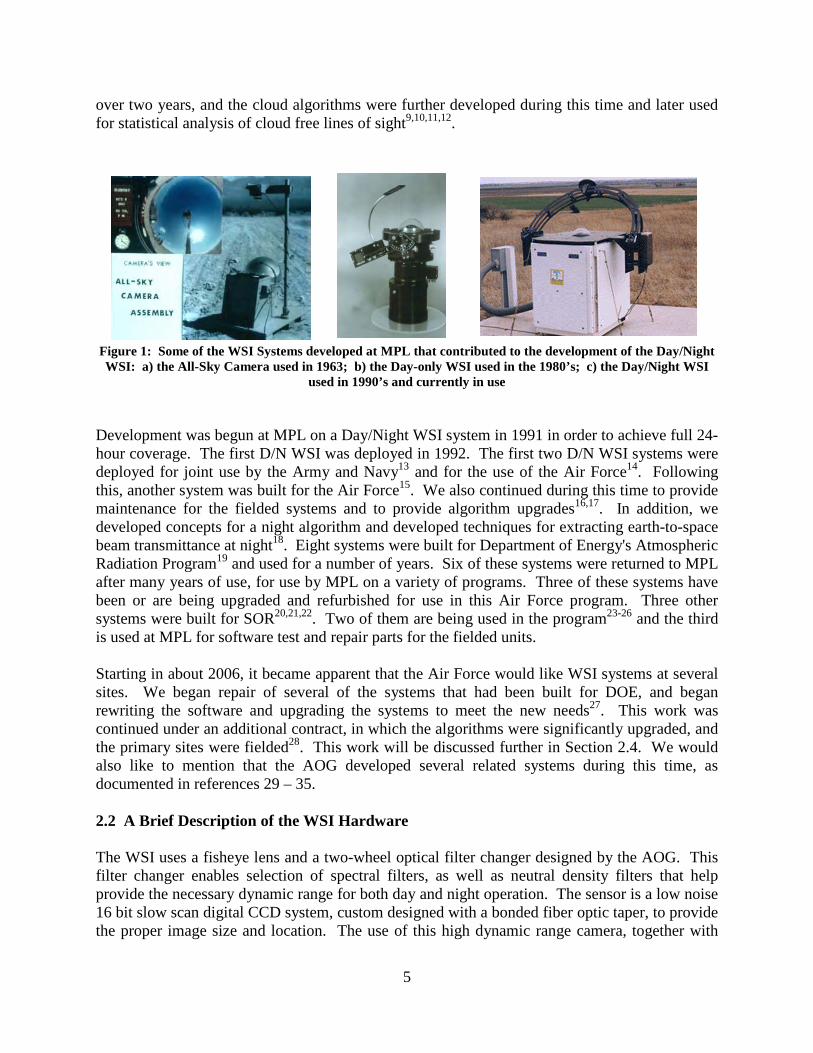
The MPL group used all-sky cameras using film and a silvered mirror in the 1960's (Figure 1a), and then used film cameras with fisheye lenses in the 1970's. The automated Day-only WSI developed in the early and mid-1980’s based on CID technology is shown in Figure 1b, and the Day/Night WSI used starting in the 1990's is shown in Figure 1c. To the best of our knowledge, the systems developed by the MPL group were the first digital or automated WSI systems, and the Day/Night WSI systems were the first, and remain the only visible WSI systems with full diurnal coverage. The first MPL digital WSI was fielded at White Sands Missile Range in 1984. Cloud algorithms based on the red/blue ratio at each pixel were developed in 19861. The Day WSI system shown in Figure 1b was hardened and automated, and fielded at 7 sites starting in 19881,2,3. Data were acquired at several sites at 1-minute intervals for

5

over two years, and the cloud algorithms were further developed during this time and later used for statistical analysis of cloud free lines of sight9,10,11,12.

Figure 1: Some of the WSI Systems developed at MPL that contributed to the development of the Day/Night WSI: a) the All-Sky Camera used in 1963; b) the Day-only WSI used in the 1980’s; c) the Day/Night WSI

used in 1990’s and currently in use Development was begun at MPL on a Day/Night WSI system in 1991 in order to achieve full 24-hour coverage. The first D/N WSI was deployed in 1992. The first two D/N WSI systems were deployed for joint use by the Army and Navy13 and for the use of the Air Force14. Following this, another system was built for the Air Force15. We also continued during this time to provide maintenance for the fielded systems and to provide algorithm upgrades16,17. In addition, we developed concepts for a night algorithm and developed techniques for extracting earth-to-space beam transmittance at night18. Eight systems were built for Department of Energy's Atmospheric Radiation Program19 and used for a number of years. Six of these systems were returned to MPL after many years of use, for use by MPL on a variety of programs. Three of these systems have been or are being upgraded and refurbished for use in this Air Force program. Three other systems were built for SOR20,21,22. Two of them are being used in the program23-26 and the third is used at MPL for software test and repair parts for the fielded units. Starting in about 2006, it became apparent that the Air Force would like WSI systems at several sites. We began repair of several of the systems that had been built for DOE, and began rewriting the software and upgrading the systems to meet the new needs27. This work was continued under an additional contract, in which the algorithms were significantly upgraded, and the primary sites were fielded28. This work will be discussed further in Section 2.4. We would also like to mention that the AOG developed several related systems during this time, as documented in references 29 – 35. 2.2 A Brief Description of the WSI Hardware The WSI uses a fisheye lens and a two-wheel optical filter changer designed by the AOG. This filter changer enables selection of spectral filters, as well as neutral density filters that help provide the necessary dynamic range for both day and night operation. The sensor is a low noise 16 bit slow scan digital CCD system, custom designed with a bonded fiber optic taper, to provide the proper image size and location. The use of this high dynamic range camera, together with

6

the changes in exposure and neutral density and spectral filters enables a net dynamic range of over 10 logs (1010). An environmental housing provides protection for the camera electronics unit, the camera cooling elements, and other components that provide real time readout of system conditions. A solar/lunar occultor provides shading for the lens and dome. The occultor operates with an arc that moves East to West. Some of the WSI systems have a trolley system that moves from North to South, to cover the sun or moon, and others have a shade that covers the north-south extent of the sun and moon positions. System electronics called the Accessory Control Panels (ACP) enable both manual and computer control of the filter changer and occultor, as well as system readouts such as camera chip temperature and camera housing temperature. Custom system control software designed and developed by MPL controls the occultor, determining sun or moon location with GPS input to determine time and location. The software controls the exposures and filter settings, according to sun and moon position, moon phase, and other related parameters. The software provides all control functions including data acquisition and checking of status parameters that allow the computer to turn off the camera if it is too hot or otherwise at risk. A separate processing computer on each system provides real time application of the cloud algorithms that generate the cloud decision (or “cloud mask”). In addition, the computer provides additional automated QC designed to provide assessments of data presence and quality. It sends the data by ftp to SOR as well as providing separate archival. It monitors the control computer and will reboot if necessary. 2.3 The Cloud Algorithms and their Development at MPL The first cloud algorithm developed in 1984-86 was based on ratios of red and blue images1. Initial cloud algorithms used a fixed threshold for red/blue calibrated ratio9. In the late 80’s, a thin cloud algorithm was developed to better account for variations in thin cloud spectral signature10. In recent years, the algorithm has been updated to include a night algorithm, upgrades to the day algorithm, and evaluation of cloud free line of sight23,24,25,26. Day algorithm upgrades included adapting it for the current hardware configuration, identifying the occultor and obstructions in the image as “no data”, providing better handling of the calibration characteristics, and providing better handling of haze. One of the important changes was to optionally use Near Infrared (NIR) images, as this wave band receives less scattered light from the small droplet haze or aerosols, in comparison with the large droplet thin clouds. The first night algorithm concepts were based on detecting stars by evaluating the contrast between stars in the image and the sky background. Later versions were based on determining the absolute transmittance Tr of the atmosphere in the direction of the stars. A high resolution night algorithm was developed and fielded in early 2007 based on the earlier techniques combined with the use of the radiance distribution. At the start of this contract, this version was still in development, particularly for moonlight. Sample algorithm results are provided in Figures 2 – 4. In the cloud decision images, blue indicates no cloud, and white-to-grey indicates opaque cloud. Thin cloud is indicated with yellow in the day and green at night, and black indicates no data.

7

Figure 2: Raw and cloud decision images Day/Night WSI taken Figure 3: Color code for Fig. 2 under sunlight (19 May 06 1700Z)

2.4 Summary of Most Recent Work Prior to the Contract The most recent work prior to the start of this contract was done for the Naval Post Graduate School (NPS) and in association with Starfire Optical Range (SOR), Kirtland Air Force Base, under NPS/FISC Grant N00244-07-1-0009, between 28 June 2007 and 31 October 2008. Under this prior contract, we completed the refurbishment of 3 WSI systems, and completed deployment of the units to the 3 primary test sites. We completed the upgrade of the daytime cloud algorithm in order to include an adaptive feature that adjusted for haze amount. We completed the upgrade of the nighttime cloud algorithm in order to provide results at high resolution under both starlight and moonlight, although additional features were added later. This work, as well as a detailed summary of previous contract work, is reported in the report for that contract28.

Figure 4: Raw image, cloud decision image, and transmittance map from the D/N WSI taken under starlight,

i.e. no moon, (26 May 06 1918Z)

Tr with Aerosol

correction> 1.0

0.8 – 1.0 0.6 - 0.8 0.4 - 0.6 0.2 - 0.4 0.0 - 0.2 Star Not

detected

8

2.5 Purpose of the Current Contract Under the current contract, our initial goals were to acquire a good data base of cloud images, at 3 primary data sites, and two secondary sites, with data acquired once a minute during the day time and every two minutes at night. We developed high accuracy algorithms to enable us to process the raw imagery to provide cloud decision results similar to the cloud images shown in Figures 3 and 4, and to provide the data in digital format. (Much of the algorithm development was completed under the previous contract). Then we processed all of the data acquired at the primary three sites, and much of the data acquired at one of the secondary sites. Initially, the contract was set up as a 5-year contract, and additional development was intended. . However the program was cancelled due to funding constraints and through no fault of either MPL or SOR, only a year into the 5-year contract. We were enabled by SOR to complete 1 year and 11 months of work (and were funded for 1.2 years of the original budget). In spite of this, we are very pleased to have completed the development of the algorithms, and providing the large data base of processed data. This will be discussed in this report, as well as other tasks that were completed. While we had intended to use the data base for analysis including forecasting of cloud free line of sight, studies of typical optical fade through clouds, and so on, it is good to have the data available in case these studies are needed in the future. 2.6 A Note on References One of the requirements of this contract is to provide short reports on the algorithm analysis for the various data periods at each site, on software upgrades, on repair procedures, and so on. These reports were generally provided in the form of technical memoranda. In addition, we wrote technical memoranda documenting things like software that’s used in-house, trip reports, and other areas we felt were important to the program. Although these memos cannot be listed as formal references, because they are not readily available to the public, we have listed them in Appendix 1, and will refer to them in the text. The memos are available to the sponsors, and we are happy to evaluate requests from others.

9

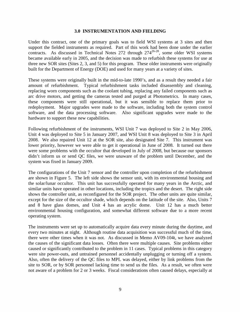
3.0 INSTRUMENTATION AND FIELDING Under this contract, one of the primary goals was to field WSI systems at 3 sites and then support the fielded instruments as required. Part of this work had been done under the earlier contracts. As discussed in Technical Notes 272 through 27426-28, some older WSI systems became available early in 2005, and the decision was made to refurbish these systems for use at three new SOR sites (Sites 2, 3, and 5) for this program. These older instruments were originally built for the Department of Energy (DOE) and used for many years at a variety of sites. These systems were originally built in the mid-to-late 1990’s, and as a result they needed a fair amount of refurbishment. Typical refurbishment tasks included disassembly and cleaning, replacing worn components such as the coolant tubing, replacing any failed components such as arc drive motors, and getting the cameras tested and purged at Photometrics. In many cases, these components were still operational, but it was sensible to replace them prior to redeployment. Major upgrades were made to the software, including both the system control software, and the data processing software. Also significant upgrades were made to the hardware to support these new capabilities. Following refurbishment of the instruments, WSI Unit 7 was deployed to Site 2 in May 2006, Unit 4 was deployed to Site 5 in January 2007, and WSI Unit 8 was deployed to Site 3 in April 2008. We also repaired Unit 12 at the SOR site, also designated Site 7. This instrument was lower priority, however we were able to get it operational in June of 2008. It turned out there were some problems with the occultor that developed in July of 2008, but because our sponsors didn’t inform us or send QC files, we were unaware of the problem until December, and the system was fixed in January 2009. The configurations of the Unit 7 sensor and the controller upon completion of the refurbishment are shown in Figure 5. The left side shows the sensor unit, with its environmental housing and the solar/lunar occultor. This unit has successfully operated for many years in the Arctic, and similar units have operated in other locations, including the tropics and the desert. The right side shows the controller unit, as reconfigured for the SOR project. The other units are quite similar, except for the size of the occultor shade, which depends on the latitude of the site. Also, Units 7 and 8 have glass domes, and Unit 4 has an acrylic dome. Unit 12 has a much better environmental housing configuration, and somewhat different software due to a more recent operating system. The instruments were set up to automatically acquire data every minute during the daytime, and every two minutes at night. Although routine data acquisition was successful much of the time, there were other times when it was not. As discussed in Memo AV09-104t, we have analyzed the causes of the significant data losses. Often there were multiple causes. Site problems either caused or significantly contributed to the problem in 11 cases. Typical problems in this category were site power-outs, and untrained personnel accidentally unplugging or turning off a system. Also, often the delivery of the QC files to MPL was delayed, either by link problems from the site to SOR, or by SOR personnel lacking time to send us the files. As a result, we often were not aware of a problem for 2 or 3 weeks. Fiscal considerations often caused delays, especially at

10

the beginning of the contract, when we didn’t have repaired spares built up yet, and for the last year of the contract, when we had to curtail spending.

Figure 5: Sensor and Controller Configuration for Unit 7

In less than 20% of the cases with significant loss was the loss caused by WSI hardware problems, and not severely exacerbated by either site of fiscal issues. Of these cases, the most severe WSI instrumentation problem was caused by failures of the occultor or the occultor electronics. We had begun to address this problem with the design of a new occultor concept, which we felt would be more robust and also occult less of the sky. The other primary problem we had was that we fielded Unit 7 with one of the older style coolers, which has worked at several sites, but we found it was not adequate for Site 3, which had temperatures sometimes exceeding 120°. We had already converted some of the instruments to use a better cooler, but this experience certainly tells us that the better coolers are a necessity at some sites. In terms of problems we didn’t have any control over, e.g. site problems and fiscal problems, the recommendations we would make would be to first provide us direct access to the QC files, if feasible, so that we could determine immediately when there is a problem, and fix it promptly. Also, we feel that at least with these older instruments, it would have been helpful to have funding levels that permitted the trained personnel in our team to do the repairs. In general, we feel that the hardware worked quite well, acquiring excellent imagery much of the time. We were working on designs for a new system when the program funding was curtailed, but the old systems operated reasonably well in spite of their age and the site and funding issues.

11

4.0 DAY ALGORITHM FOR CLOUD DETERMINATION One of the goals of this contract was to complete an upgraded daytime cloud algorithm that would handle haze better. Most of this work was completed under the previous contract. The new algorithm was documented in Memo AV09-040t and Technical Note 27428, and described in somewhat less detail in this section. This section provides an overview of the day cloud algorithm, as well as the adaptive algorithm upgrade to handle variations in haze amount. The cloud algorithm is the algorithm that identifies the presence of opaque and thin clouds in each pixel. There are separate day and night algorithms; a sunset algorithm has not yet been developed. Both the day and the night algorithm are based on the following: a) The anticipated response of the atmospheric optical properties to clouds, based on atmospheric optical theory. b) The anticipated impact of the sensor system on the measurements. c) Modification as required based on the empirical behavior of the data. The driving design of the algorithm has always been the theoretical behavior of the atmospheric optics, but the algorithm also includes calibration corrections, because we recognize that no sensor is perfect, and it will have an impact on the acquired data. As we have developed the algorithm, we have also found that it is necessary to use empirical data to fine-tune the algorithm, partly because the altitude differs from one site to another. As will be described below, the day algorithm is based on either the red/blue image ratios or NIR/blue image ratios. We find that fixed ratio thresholds can be used to identify the opaque clouds, once certain calibration corrections are applied. To identify thin clouds, we characterize the typical clear sky ratio as a function of solar position and look angle in the sky, and then determine the thin clouds based on the comparison with this clear sky. Finally, a haze algorithm feature is used to detect haze amount, and adjust the algorithm accordingly. 4.1 Overview of the Day Cloud Algorithm for Opaque and Thin Clouds The day cloud algorithm uses the imagery of the sky measured with blue filters and either red or NIR filters. The initial steps in the algorithm are essentially calibration corrections, which include dark correction and non-uniformity correction. We have found that non-linearity correction is not necessary with this system, because the corrections are so small. From the corrected data, either Red/blue or NIR/blue ratios are computed at each pixel. The algorithm for opaque clouds depends on the opaque clouds having a red/blue or NIR/blue ratio greater than or equal to a given threshold, which is well above the values typically encountered for thin clouds or no clouds. This is logically equivalent to saying that opaque clouds are less blue than thin clouds, because of the enhanced multiple scattering within the clouds. Thus the ratios can be thresholded to provide detection of opaque clouds. We also check for pixels that are offscale bright or dark, or that have ratios that are offscale. In our early research, we found that this fixed threshold worked quite well for opaque clouds for all solar zenith angles, and all conditions we have encountered. Originally, we had to apply a

12

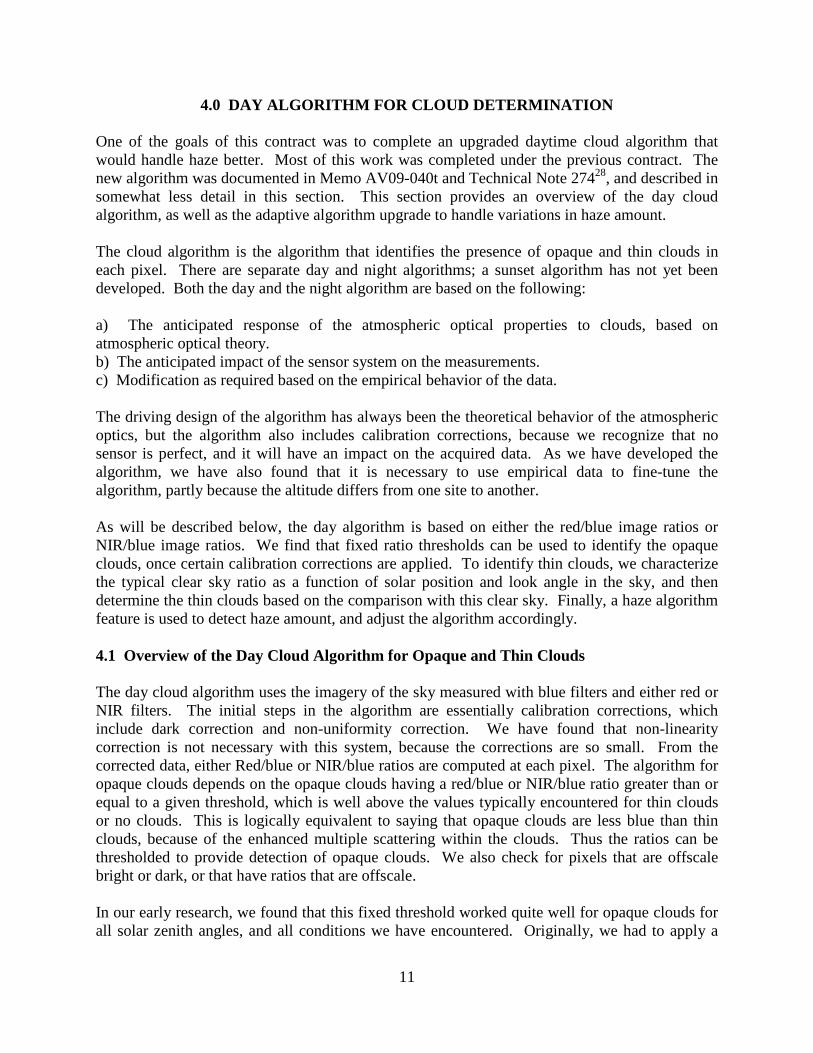
zenith-angle-dependent correction. However under the previous contract, we added the non-uniformity calibration correction, and as a result we no longer have to apply an additional zenith-angle-dependent correction. Thus the zenith-dependent correction we applied previously appears to be due to filter and lens effects that are corrected with the uniformity correction, rather than atmospheric optical effects. Thin clouds can be better described as having a ratio that’s slightly higher than the normal clear sky ratio (as opposed to a fixed ratio such as is used with the opaque clouds). Accordingly, techniques were developed several years ago to characterize the clear sky ratio as a function of look angle and solar zenith angle. This clear sky background ratio is extracted from cloud-free images acquired at the site in the field, and stored as a file of normalized ratios as a function of solar zenith angle and look angle. When field data are processed, a clear sky background ratio image is generated for each field image, based on the current solar zenith angle. This clear sky background image is also normally adjusted in magnitude as a function of solar zenith angle. As we extract the clear sky background, we normalize these images based on the average ratio at two points in each image. These two points are at the intersection of the circle around the sun representing a scattering angle beta of 45 degrees and a circle in the image representing a zenith angle theta of 45 degrees. We refer to these as the “beta points”. In extracting these normalization points used in the clear sky background, we visually ensure that only cloud-free points are extracted. Figure 6 shows the magnitude of the average ratio at the two beta points, for a number of reasonably cloud-free (both clear and hazy) days, and as a function of solar zenith angle. It rises very strongly near sunrise and sunset, corresponding with the whiter (or redder) skies we encounter at these times. Also note that the magnitude of the curve varies somewhat from one day to another. It turns out that this variation is a result of variations in haze amount. When the sky is hazier, the ratios at these beta points are higher. In Figure 6, there are 3 best fit curves, corresponding with a hazy sky, a typical sky, and a very clear sky (relative to conditions encountered at the site). In the previous version of the algorithm, we could choose a single best fit curve to use for the data set. As a result, the changes in the normalization constant as a function of Solar Zenith Angle (SZA) were well handled, but the day-to-day changes resulting from changing haze amount were not handled. Once the clear sky background image has been generated, those pixels in the current ratio image that are not identified as opaque or offscale are compared with the clear sky ratio. A perturbation ratio is computed for each pixel. This perturbation ratio is the ratio of the current pixel red/blue or NIR/blue ratio divided by the clear sky background library ratio. (The perturbation ratio shows how much the current ratio is perturbed or changed with respect to a the clear sky background library ratio for this site, time, and direction.) If the perturbation ratio exceeds a threshold (typically 1.2 or a 20% change), then the pixel is identified as thin cloud. Also, if the clear sky background ratio is higher than the opaque threshold, the pixel will be identified as “indeterminate”, meaning that the clear sky ratio in this direction for this solar zenith angle is anticipated to be higher than the ratio for opaque clouds, and thus we can’t identify whether there are clouds there based on spectral signature alone. Memos AV06-018t and -020t show results of this earlier algorithm for two sites.

13

Figure 6: Reference Values, or Normalization Values, for clear sky ratios during several cloud-free

(or nearly cloud-free) days at Site 5. 4.2 The Adaptive Algorithm Upgrade for Haze In the past, we have found that occasionally under heavy haze, the algorithm identifies the cloud-free sky as thin cloud. Haze will in fact attenuate the signal of anything such as a laser going through the atmosphere, just as thin clouds will, but unlike clouds, it attenuates much less in the Short Wave IR than in the visible due to the smaller drop sizes. As a result, we want to be able to distinguish haze from thin cloud, since many applications are in non-visible wavelengths. We have found that enhanced haze causes the radiances to be higher in both filters, and also causes the ratio to be higher, as illustrated in Figure 6. Although haze impacts the magnitude of the clear sky background ratio, we have found from both modeling and image evaluation that it does not significantly affect the shape of the clear sky background (i.e. its variation with look angle), except for modest changes in the aureole and near the horizon. To take advantage of this behavior, we developed logic that evaluates the perturbation ratio along a line in the image between the two beta points in order to determine whether the clear sky ratio should be adjusted up or down for that image. The logic is somewhat complex, as it includes logic to only use segments of the line free of either opaque of thin cloud. It also includes

14

logic to avoid the solar aureole, where the perturbation ratios may be atypical due to variations in the drop size distribution. Based on the results in these line segments, a correction is determined if possible, and applied to the clear sky background for the whole image. If we are unable to determine a correction for a given image, then the most recent correction is adjusted for the change in SZA (using the curves in Figure 6), and applied to the current image. Also in Figure 6 note that in general if a given image has a higher or lower reference value than average, it tends to stay that way, to a first approximation, throughout a day. That is, the green curves all stay somewhere near the upper curve, and the blue curve stays near the middle curve, with occasional exceptions as demonstrated by the bottom orange curve. This implies that in general optical characteristics as influenced by the haze amount tend to persist for at least a few hours. As a result, using the most recent correction adjusted for SZA generally works quite well. We find that when there are significant errors, it’s because the haze has changed somewhat, but there are thin clouds present that prevent a new determination, so the thin clouds threshold is not quite right. This means that some thin cloud is erroneously identified as no cloud, or some of the clear sky is erroneously identified as cloud. This only happens rarely, and it may be possible to further improve the algorithm in the future to handle this situation. Figure 7 shows a sample when the day was significantly hazier than the nominal clear day. The green curve shows the magnitude of the field image red/blue ratio along the line, and the purple curve shows the magnitude of the clear sky library ratio along the line. The algorithm chose a correction factor of 1.42 for this case.

Figure 7: Sample results for an image on a cloud-free day with high haze amount

15

The next question is how well the haze correction factor determined from the beta line applies to the whole image. In Figure 8, we have shown the field ratio and the clear sky ratio, both for the beta line, and for a line going through the sun. As can be seen in Figure 8, the separation between the green and purple lines for the beta line (plot on the left) appears to be reasonably representative of the separation that occurs on a line through the sun and the horizon. That is, the perturbation ratio along the beta line appears to represent the perturbation for other parts of the image quite well. This indicates that the haze correction determined using the beta line should apply reasonably well to the full image. We found that this was the case; that is, the correction works quite well over the whole image in most cases.

Figure 8: Red/blue ratio for the current image (green line) and its nominal clear sky background

(purple line); plot on left is for beta line, and plot on right is for line through the sun; this is for a relatively high haze case

4.3 Evaluation of the Adaptive Algorithm Results Although the adaptive algorithm was developed mostly under the previous contract, we had the opportunity to evaluate extensive data from several sites under this contract. We found that the new algorithm worked quite well nearly all the time for clear skies, hazy skies, thin cloud conditions, broken, and overcast conditions. Several examples will be shown in later sections. One example for a hazy day with broken clouds is shown in Figure 9, which shows a raw image, the result without use of the adaptive algorithm and the much-improved result with the adaptive algorithm. Note in the bottom right image of Figure 9 that there is a grey circle around the sun.

16

This is a region characterized as “indeterminate”. In these pixels, the clear sky background, as adjusted for the high haze, has a high enough ratio that it cannot readily be separated from opaque cloud, so the small region is identified as indeterminate.

Raw image, 9 May 08 1700

Result without adaptive feature of algorithm Result with adaptive algorithm

Figure 9: Sample result for broken clouds, 9 May 08 1700 The Site 5 Jan – May 2008 data set was used to develop the adaptive algorithm. To further test the results of the adaptive algorithm, we ran an additional run with the same input parameters, but with the adaptive feature of the algorithm turned off. We evaluated the hourly data, and found that out of 1401 cases we evaluated, approximately 24% of the cases were significantly better with the adaptive algorithm turned on. Approximately 74% were good with either algorithm, and approximately 2% of the cases were significantly worse with the adaptive

17

algorithm turned on. Most of the cases in which the algorithm did better were in April and May, and were the heavy haze cases. We would not expect this much improvement at relatively haze-free sites. Most of the cases in which the algorithm results were not as good were cases in which there was cirrus, and the algorithm did not pick up as much of the cirrus as it should have, although it generally picked up some. In summary, the new adaptive algorithm evaluates the images on a case by case basis, to adjust for the impact of haze on the image. If it cannot make a current determination, it uses the most recent determination, as corrected for changing solar zenith angle. We found that the new algorithm is not perfect, but is much better than the previous version, and generally does a very nice job under all conditions. Further examples will be shown in Section 7, and evaluation of the accuracy is further discussed in Section 8. It should also be noted that during this contract, we updated many of the programs used to handle the data, extract the day algorithm inputs, process the data, and test and evaluate the results. These upgrades are documented in various memos listed in Appendix 1.

18

5.0 NIGHT ALGORITHM FOR CLOUD DETERMINATION One of the goals in this contract was to complete the night algorithm. Most of this work was completed under the previous contract, although we did add additional logic to handle stray lights and to handle the Milky Way better at very dark sites under this contract. The new algorithm was documented in Memo AV09-056t and Technical Note 27428, and described in somewhat less detail in this section. This section provides an overview of the night cloud algorithm, as well as the additions to handle moonlight at high resolution. 5.1 Overview of the Night Cloud Algorithm Development and Logic Early versions of the night algorithm were based on evaluating the presence of stars within small regions of the sky. These algorithms used star libraries and high accuracy angular calibration to identify the presence (or lack thereof) of stars in the image. Results were provided in each of 357 cells over the sky. More recently, the algorithm was upgraded to provide nearly full resolution results. Although the result is at full pixel resolution, a 5 x 5 smoothing of the image is used during part of the processing, so we refer to it as a “high resolution” algorithm. We initially fielded a version at Site 2 that worked for starlight, but was not yet adapted for moonlight. Under the previous contract, we developed the moonlight feature. Under this contract, we further improved the high resolution algorithm, as we were able to evaluate large data sets from several sites. The night cloud algorithm is based on the “open hole” images that are acquired at night. These images are filtered by the response curve of the CCD, as well as a NIR blocking filter, but they are relatively broad band, in comparison with the daytime images which use 70 nm passband spectral filters. The first major step in the algorithm is applying the absolute radiance calibration. This step converts the raw image to absolute radiance floating point values, based on the radiometric calibrations acquired in the lab. This also includes the dark image correction and uniformity correction. Linearity corrections are not applied at the present time, as they are generally quite small (typically 1%, worst case about 4%). The 5th edition NSSDC Bright Star Catalog36 is used to provide the location, magnitude, and color temperature of the stars. We developed techniques to use the star magnitude and color temperature, and determine the inherent radiance of the star (above the atmosphere) in the WSI passband. These techniques are documented in earlier memos and reports18, 21, 23. Techniques were developed to provide a high accuracy angular calibration of the WSI imagery, typically accurate to about half a pixel or 1/6 degree. Using the anticipated angular position of stars, and the angular calibration of the imagery, we detect the stars in the images, and compute their apparent irradiance, i.e. irradiance as measured from the ground. This apparent irradiance is determined using a best fit routine that models the signal in the vicinity of the star as a Gaussian with a point spread function of approximately 0.4 pixel width. From this best fit, and the radiances of each pixel, the algorithm removes the background radiance, and determines the apparent irradiance of the star.

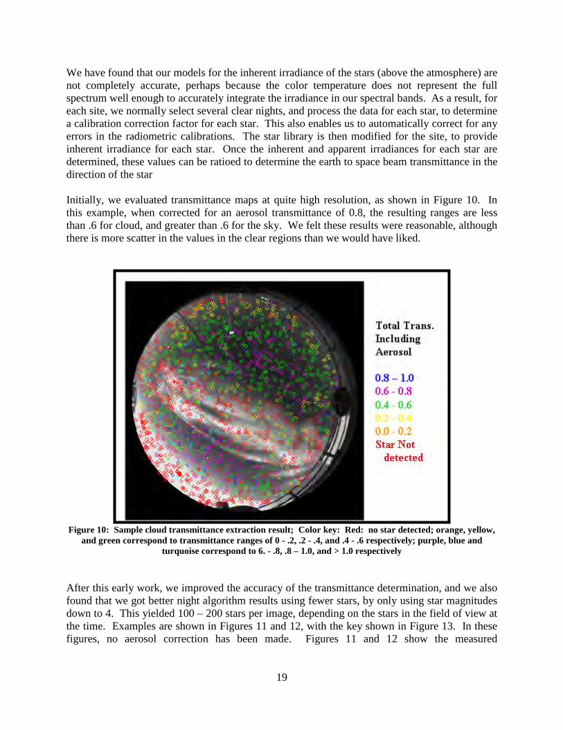
19

We have found that our models for the inherent irradiance of the stars (above the atmosphere) are not completely accurate, perhaps because the color temperature does not represent the full spectrum well enough to accurately integrate the irradiance in our spectral bands. As a result, for each site, we normally select several clear nights, and process the data for each star, to determine a calibration correction factor for each star. This also enables us to automatically correct for any errors in the radiometric calibrations. The star library is then modified for the site, to provide inherent irradiance for each star. Once the inherent and apparent irradiances for each star are determined, these values can be ratioed to determine the earth to space beam transmittance in the direction of the star Initially, we evaluated transmittance maps at quite high resolution, as shown in Figure 10. In this example, when corrected for an aerosol transmittance of 0.8, the resulting ranges are less than .6 for cloud, and greater than .6 for the sky. We felt these results were reasonable, although there is more scatter in the values in the clear regions than we would have liked.

Figure 10: Sample cloud transmittance extraction result; Color key: Red: no star detected; orange, yellow,

and green correspond to transmittance ranges of 0 - .2, .2 - .4, and .4 - .6 respectively; purple, blue and turquoise correspond to 6. - .8, .8 – 1.0, and > 1.0 respectively

After this early work, we improved the accuracy of the transmittance determination, and we also found that we got better night algorithm results using fewer stars, by only using star magnitudes down to 4. This yielded 100 – 200 stars per image, depending on the stars in the field of view at the time. Examples are shown in Figures 11 and 12, with the key shown in Figure 13. In these figures, no aerosol correction has been made. Figures 11 and 12 show the measured

20

transmittances for the stars for two cases at 0530 and 0626, on 2 June 2008 at Site 5. There is some thin cloud in Figure 11, and more in Figure 12, with correspondingly lower transmittances.

Figure 11: Transmittance map for 2 June 2008 0530 Figure 12: Transmittance map for 2 June 2008 0626

Figure 13: Key for Transmittance maps

Once the earth-to-space beam transmittance is determined for each star (or it is determined that the star cannot be detected), complicated logic and thresholds are used to label each star location as either no cloud, thin cloud, or opaque cloud. 5.2 Using the Radiance Distribution to extend to High Resolution In order to extend these determinations made at the star positions to all pixels, it is necessary to use the calibrated radiances. Prior to processing the field data, as part of setting up the

21

algorithm, we do extensive analysis of the calibrated radiance images for clear and cloudy skies, for no moon and for moonlight. It is beyond the scope of this report to provide the details of this procedure, although some details are provided below, and more are in Technical Note 27428. As a result of this pre-analysis procedure, we characterize the typical anticipated shape of the sky radiance distribution, for the above-named conditions. For the starlight case, the no-cloud distribution is also a function of the hour angle, and for the moonlight case, the no-cloud distribution also depends strongly on the moon position, phase, and earth-to-moon distance. We refer to these radiance distributions as “shells”. Samples of these shells will be illustrated below, but first we need to explain one more feature of the algorithm. At each star location, once we identify it as no cloud, thin cloud, or opaque cloud, then we also determine the background radiance at that location, i.e. the radiance of the sky or cloud near the star. If the star location was identified as clear sky, these background radiances are used, for each image, to adaptively adjust the clear sky shell. Similarly, if the star location was identified as opaque cloud, the background radiance is used to adaptively adjust the opaque cloud shell. Once current shells for no cloud and cloud have been determined for the current image, then the radiance at each pixel can be compared with the shell radiances to determine whether that pixel should be identified as no cloud, thin cloud, or opaque cloud. In Figure 14, we show the raw image on the left, and the algorithm result on the right. In Figure 15, we show the shells and the measured radiances. The orange curve is the anticipated radiance for no moon (starlight) and no cloud, for Column 255, through the approximate center of the image. The green curve shows the anticipated radiance, or shell, for the moon alone for the same column. The sum of these two curves forms the nominal shell for no cloud, prior to the adaptive adjustment, and is not shown in the figure.

Figure 14: Raw Image and Cloud Algorithm Results for Site 5, 2 June 2007, 0656 GMT

The black curve shows the measured radiance for the same central column. From those stars that were identified as no cloud, for this image, an adaptive correction factor of 1.13 was determined.

22

The blue curve shows the clear sky shell with the adaptive factor applied. In the algorithm, any pixel with a radiance 15% higher than the clear sky shell was identified as thin cloud.

Figure 15: Model and Measured Radiances, with Adaptive Corr 1.13 for Site 5, 2 June 2007, 0656 GMT

In the above example, the opaque cloud shell was well above the level of the measured radiances, and was not shown in the plot. A second example, this time with no moon, is provided below, and includes the opaque cloud shell. In Figure 16, we see the raw image and the cloud decision image for a no moon case with mixed clouds.

Figure 16: Raw Image and Cloud Algorithm Results

for a case with no moon, Site 5, 20 June 2007, 0716 GMT Figure 17 shows the plots of the cloud shells for this example. In this case, since there is no moon, the clear shell consists only of the starlight no moon shell for the appropriate hour angle. (It is not shown.) Using the background radiance in the region of the stars identified as no cloud,

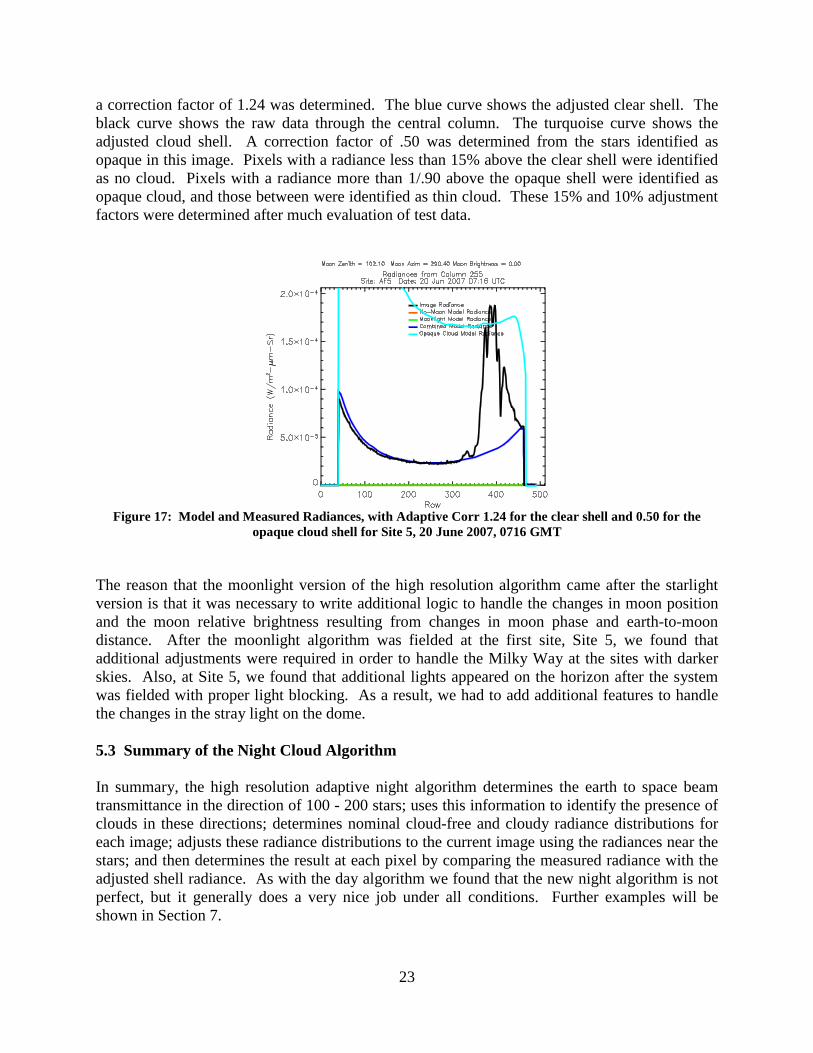
23

a correction factor of 1.24 was determined. The blue curve shows the adjusted clear shell. The black curve shows the raw data through the central column. The turquoise curve shows the adjusted cloud shell. A correction factor of .50 was determined from the stars identified as opaque in this image. Pixels with a radiance less than 15% above the clear shell were identified as no cloud. Pixels with a radiance more than 1/.90 above the opaque shell were identified as opaque cloud, and those between were identified as thin cloud. These 15% and 10% adjustment factors were determined after much evaluation of test data.

Figure 17: Model and Measured Radiances, with Adaptive Corr 1.24 for the clear shell and 0.50 for the

opaque cloud shell for Site 5, 20 June 2007, 0716 GMT The reason that the moonlight version of the high resolution algorithm came after the starlight version is that it was necessary to write additional logic to handle the changes in moon position and the moon relative brightness resulting from changes in moon phase and earth-to-moon distance. After the moonlight algorithm was fielded at the first site, Site 5, we found that additional adjustments were required in order to handle the Milky Way at the sites with darker skies. Also, at Site 5, we found that additional lights appeared on the horizon after the system was fielded with proper light blocking. As a result, we had to add additional features to handle the changes in the stray light on the dome. 5.3 Summary of the Night Cloud Algorithm In summary, the high resolution adaptive night algorithm determines the earth to space beam transmittance in the direction of 100 - 200 stars; uses this information to identify the presence of clouds in these directions; determines nominal cloud-free and cloudy radiance distributions for each image; adjusts these radiance distributions to the current image using the radiances near the stars; and then determines the result at each pixel by comparing the measured radiance with the adjusted shell radiance. As with the day algorithm we found that the new night algorithm is not perfect, but it generally does a very nice job under all conditions. Further examples will be shown in Section 7.

24

Further details on most steps of the algorithm can be found in the references below provided earlier, including the more recent technical reports26, 27, 28 and several of the technical memos listed in Appendix 1.

25

6.0 NIGHT BEAM TRANSMITTANCE PRODUCT AND OPTICAL FADE Our SOR sponsors have been interested in using the WSI to determine the optical density of the clouds, night and day. We developed this capability for nighttime, and presented the results in May 2008. The results were not automated as part of the archive processing until toward the end of the program, however, because this was lower priority than getting the data archive processed. For daytime, we developed concepts to extract the optical density, as documented in Memo AV08-053t, but were told that this should not be a priority. In this section, we present sample night transmittance results. 6.1 Definition of Transmittance-related Terms To define our terms, if a laser beam with power P1 is incident on a cloud, and power P2 is successfully transmitted through the cloud, then the transmittance, optical fade, and optical depth can be defined by Equations 1 – 3. (1) (2) (3) In these equations, RT is defined as transmittance over path length R, n is defined as optical fade in dB, and δ is defined as optical depth. Sample values of these parameters are shown in Table 1. The first 3 rows show the transmittance and optical depth associated with a dB fade of 1, 2, and 3 dB. The last 3 rows show values associated with comments made in meetings, related to the definition of nominal thin clouds, the pyranometer threshold, and the definition of opaque clouds. The last comes from a casual remark that 6 dB is considered “not quite opaque by some”.

Table 1 Comparison of Various Transmittance-related Parameters

dB Fade Trans Opt Depth Comment

1 .794 .23 2 .631 .46 3 .501 .69

.13 – 1.3 .97 - .74 .03 - 0 .3 Nominal thin cirrus 2 – 4 .63 - .40 .46 - .92 Nominal Pyranometer threshold

6 .25 1.4 “Not quite opaque” An overview of the development of the night transmittance capability is discussed in Memo AV09-097t, and much of it is discussed in more detail in Technical Note 27428. In this earlier

δ−− === ePPT nR

1012 10)(

)log(10 12 PPn =

rTln−=δ

26

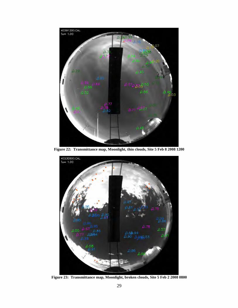
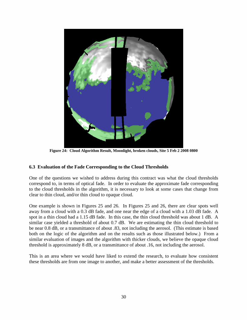
report, we report the initial transmittance maps generated in 2004 (such as shown in Figure 10 of this technical note), and tests done in 2005 to test the accuracy of these results. For bright stars, we determined that the transmittances were valid to an uncertainty of approximately ±5% over a range from about .05 to .95 transmittance (13 to 0.2 dB). We also evaluated time series, and found them to be reasonable. These results were presented to the sponsors in January 2006, and are documented in Technical Note 27327. 6.2 Sample Transmittance Maps and Discussion At the present time, we are using stars with magnitude down to 4, which typically yields 100 to 200 stars, depending on which stars are in the image. Several sample results are shown below, and additional cases are shown in Memo AV09-097t. These maps show total transmittance, not corrected for aerosol, and not corrected for zenith angle. That is, they show the actual loss in the given direction, as opposed to the loss that might have occurred if the cloud had been overhead, because for this program we care about actual losses, not the theoretical overhead losses. From the data shown below and similar data, we believe that we are measuring losses up to at least 10 dB. Based on the observed standard deviations for specific stars on clear nights, we believe our accuracy for stars to magnitude 4 is approximately 0.4 dB, or a transmittance of 0.94. We feel these results are excellent. Sample no-moon or starlight results are shown in Figures 18 - 20. Figure 18 shows a clear result. The aerosol transmittance near the zenith is about .88 to .91, or -0.5 dB (or 0.5 dB loss). Other results appear to be reasonable, and the transmittance drops off at slant angles as the path of sight goes through more atmosphere. Figure 19 shows a case with variable cloud. The orange asterisks represent stars that were not detected. The transmittances marked in yellow have fades ranging from about 7 to 15 dB relative to the aerosol. Figure 20 shows a broken cloud case, in which most of the stars were not detected, and their line of sight would be identified as opaque cloud. The threshold corresponding with “not detected” depends on the magnitude of the star, but this logic has not yet been formalized. Sample moonlight results are shown in Figures 21 - 23. Figure 21 shows a clear sky case. Like the no moon case shown in Figure 18, it resulted in aerosol losses of about 0.5 dB near the zenith. Figures 22 and 23 show cases with thin cloud and with broken opaque cloud. In Figure 22, the thin clouds have fades of about 0.3 to 4 dB relative to the aerosol over most of the sky. We show the cloud decision result corresponding to Figure 23 in Figure 24. This result is not unusual in any way, but it is such a pretty case, we felt it was worth including.

27

Figure 18: Transmittance map, No moon, clear sky, Site 5 Feb 12 2008 0800

Figure 19: Transmittance map, No moon, variable clouds, Site 5 Feb 10 2008 0200

28

Figure 20: Transmittance map, No moon, broken clouds, Site 5 Feb 14 2008 0900

Figure 21: Transmittance map, Moonlight, clear sky, Site 5 Feb 3 2008 0700

29

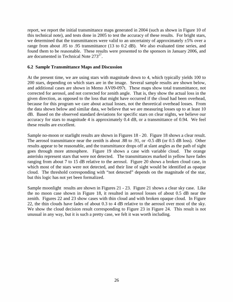
Figure 22: Transmittance map, Moonlight, thin clouds, Site 5 Feb 8 2008 1200

Figure 23: Transmittance map, Moonlight, broken clouds, Site 5 Feb 2 2008 0800

30

Figure 24: Cloud Algorithm Result, Moonlight, broken clouds, Site 5 Feb 2 2008 0800

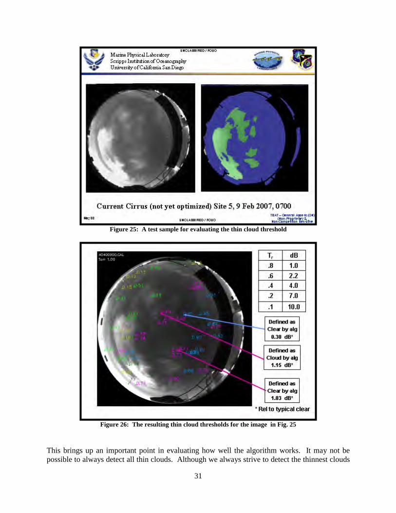
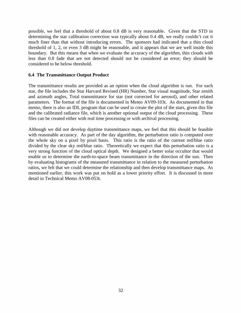
6.3 Evaluation of the Fade Corresponding to the Cloud Thresholds One of the questions we wished to address during this contract was what the cloud thresholds correspond to, in terms of optical fade. In order to evaluate the approximate fade corresponding to the cloud thresholds in the algorithm, it is necessary to look at some cases that change from clear to thin cloud, and/or thin cloud to opaque cloud. One example is shown in Figures 25 and 26. In Figures 25 and 26, there are clear spots well away from a cloud with a 0.3 dB fade, and one near the edge of a cloud with a 1.03 dB fade. A spot in a thin cloud had a 1.15 dB fade. In this case, the thin cloud threshold was about 1 dB. A similar case yielded a threshold of about 0.7 dB. We are estimating the thin cloud threshold to be near 0.8 dB, or a transmittance of about .83, not including the aerosol. (This estimate is based both on the logic of the algorithm and on the results such as those illustrated below.) From a similar evaluation of images and the algorithm with thicker clouds, we believe the opaque cloud threshold is approximately 8 dB, or a transmittance of about .16, not including the aerosol. This is an area where we would have liked to extend the research, to evaluate how consistent these thresholds are from one image to another, and make a better assessment of the thresholds.

31

Figure 25: A test sample for evaluating the thin cloud threshold

Figure 26: The resulting thin cloud thresholds for the image in Fig. 25

This brings up an important point in evaluating how well the algorithm works. It may not be possible to always detect all thin clouds. Although we always strive to detect the thinnest clouds

32

possible, we feel that a threshold of about 0.8 dB is very reasonable. Given that the STD in determining the star calibration correction was typically about 0.4 dB, we really couldn’t cut it much finer than that without introducing errors. The sponsors had indicated that a thin cloud threshold of 1, 2, or even 3 dB might be reasonable, and it appears that we are well inside this boundary. But this means that when we evaluate the accuracy of the algorithm, thin clouds with less than 0.8 fade that are not detected should not be considered an error; they should be considered to be below threshold. 6.4 The Transmittance Output Product The transmittance results are provided as an option when the cloud algorithm is run. For each star, the file includes the Star Harvard Revised (HR) Number, Star visual magnitude, Star zenith and azimuth angles, Total transmittance for star (not corrected for aerosol), and other related parameters. The format of the file is documented in Memo AV09-103t. As documented in that memo, there is also an IDL program that can be used to create the plot of the stars, given this file and the calibrated radiance file, which is another optional output of the cloud processing. These files can be created either with real time processing or with archival processing. Although we did not develop daytime transmittance maps, we feel that this should be feasible with reasonable accuracy. As part of the day algorithm, the perturbation ratio is computed over the whole sky on a pixel by pixel basis. This ratio is the ratio of the current red/blue ratio divided by the clear sky red/blue ratio. Theoretically we expect that this perturbation ratio is a very strong function of the cloud optical depth. We designed a better solar occultor that would enable us to determine the earth-to-space beam transmittance in the direction of the sun. Then by evaluating histograms of the measured transmittance in relation to the measured perturbation ratios, we felt that we could determine the relationship and then develop transmittance maps. As mentioned earlier, this work was put on hold as a lower priority effort. It is discussed in more detail in Technical Memo AV08-053t.

33

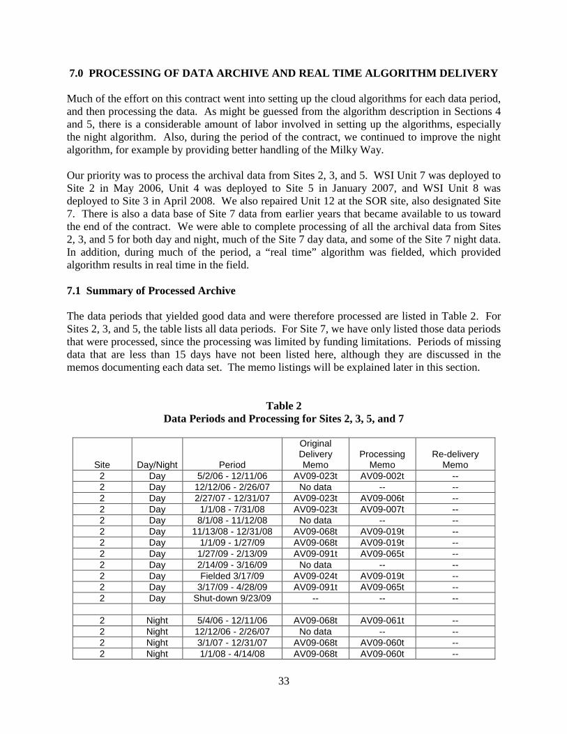
7.0 PROCESSING OF DATA ARCHIVE AND REAL TIME ALGORITHM DELIVERY Much of the effort on this contract went into setting up the cloud algorithms for each data period, and then processing the data. As might be guessed from the algorithm description in Sections 4 and 5, there is a considerable amount of labor involved in setting up the algorithms, especially the night algorithm. Also, during the period of the contract, we continued to improve the night algorithm, for example by providing better handling of the Milky Way. Our priority was to process the archival data from Sites 2, 3, and 5. WSI Unit 7 was deployed to Site 2 in May 2006, Unit 4 was deployed to Site 5 in January 2007, and WSI Unit 8 was deployed to Site 3 in April 2008. We also repaired Unit 12 at the SOR site, also designated Site 7. There is also a data base of Site 7 data from earlier years that became available to us toward the end of the contract. We were able to complete processing of all the archival data from Sites 2, 3, and 5 for both day and night, much of the Site 7 day data, and some of the Site 7 night data. In addition, during much of the period, a “real time” algorithm was fielded, which provided algorithm results in real time in the field. 7.1 Summary of Processed Archive The data periods that yielded good data and were therefore processed are listed in Table 2. For Sites 2, 3, and 5, the table lists all data periods. For Site 7, we have only listed those data periods that were processed, since the processing was limited by funding limitations. Periods of missing data that are less than 15 days have not been listed here, although they are discussed in the memos documenting each data set. The memo listings will be explained later in this section.

Table 2

Data Periods and Processing for Sites 2, 3, 5, and 7

Site Day/Night Period

Original Delivery Memo

Processing Memo

Re-delivery Memo

2 Day 5/2/06 - 12/11/06 AV09-023t AV09-002t -- 2 Day 12/12/06 - 2/26/07 No data -- -- 2 Day 2/27/07 - 12/31/07 AV09-023t AV09-006t -- 2 Day 1/1/08 - 7/31/08 AV09-023t AV09-007t -- 2 Day 8/1/08 - 11/12/08 No data -- -- 2 Day 11/13/08 - 12/31/08 AV09-068t AV09-019t -- 2 Day 1/1/09 - 1/27/09 AV09-068t AV09-019t -- 2 Day 1/27/09 - 2/13/09 AV09-091t AV09-065t -- 2 Day 2/14/09 - 3/16/09 No data -- -- 2 Day Fielded 3/17/09 AV09-024t AV09-019t -- 2 Day 3/17/09 - 4/28/09 AV09-091t AV09-065t -- 2 Day Shut-down 9/23/09 -- -- -- 2 Night 5/4/06 - 12/11/06 AV09-068t AV09-061t -- 2 Night 12/12/06 - 2/26/07 No data -- -- 2 Night 3/1/07 - 12/31/07 AV09-068t AV09-060t -- 2 Night 1/1/08 - 4/14/08 AV09-068t AV09-060t --

34

2 Night 4/15/08 - 7/31/08 AV09-068t AV09-059t -- 2 Night 8/1/08 - 11/12/08 No data -- -- 2 Night 11/14/08 - 12/31/08 AV09-068t AV09-058t -- 2 Night 1/1/09 - 1/27/09 AV09-068t AV09-058t -- 2 Night 1/28/09 - 2/13/09 AV09-091t AV09-058t -- 2 Night 2/14/09 - 3/17/09 No data -- -- 2 Night 3/18/09 - 3/31/09 AV09-091t AV09-058t -- 2 Night Fielded 3/17/09 AV09-024t AV09-058t 2 Night 4/1/09 – 9/23/09 AV09-024t AV09-058t AV09-091t 2 Night Shut-down 9/23/09 -- -- - 3 Day 4/9/08 - 8/4/08 AV08-038t AV09-008t -- 3 Day 8/5/08 - 12/31/08 AV09-068t AV09-046 -- 3 Day Fielded 10/14/08 AV09-024t AV09-057t -- 3 Day 2/18/09 – 7/1/09 AV09-091t AV09-075t -- 3 Day 7/2/09 – 7/13/09 No data -- -- 3 Day 7/14/09 – 8/15/09 AV09-091t AV09-075t -- 3 Day 8/16/09 – 9/10/09 Data bad -- -- 3 Day 9/10/09 – 9/23/09 No data -- -- 3 Day 9/24/09 Data bad -- -- 3 Day 9/25/09 – 10/25/09 No data -- -- 3 Day Shut-down 10/25/09 -- -- -- 3 Night 4/9/08 - 7/31/08 AV09-023t AV09-048t AV09-068t 3 Night 8/1/08 - 9/1/08 AV09-023t AV09-049t AV09-068t 3 Night 9/2/08 - 10/28/08 AV09-023t AV09-050t AV09-068t 3 Night 10/1/08 AV09-068t AV09-062t -- 3 Night 10/29/08- 12/31/08 AV09-068t AV09-062t -- 3 Night Fielded 12/15/08 AV09-024t AV09-050t AV09-091t 3 Night 1/1/09 – 7/1/09 AV09-024t AV09-050t AV09-091t 3 Night 7/2/09 – 7/13/09 No data -- -- 3 Night 7/14/09 – 8/15/09 AV09-024t AV09-050t AV09-091t 3 Night 8/16/09 – 9/10/09 Moon bad AV09-050t AV09-091t 3 Night 9/10/09 – 9/23/09 No Data -- -- 3 Night 9/24/09 AV09-024t AV09-050t AV09-091t 3 Night 9/25/09 – 10/25/09 No Data -- -- 3 Night Shut-down 10/25/09 -- -- -- 5 Day 2/1/07 - 7/13/07 AV09-023t AV09-009t -- 5 Day 7/14/07 - 1/15/08 No data -- -- 5 Day 1/16/08 - 5/20/08 AV08-038t AV09-042t -- 5 Day 5/21/08 - 5/22/08 AV09-023t AV09-042t -- 5 Day 5/23/08 - 6/30/08 No data -- -- 5 Day 7/1/08 - 10/31/08 AV09-023t AV09-043t -- 5 Day Fielded 10/14/08 AV09-024t AV09-043t -- 5 Day 10/31/08 – 7/7/09 AV09-091t AV09-074t -- 5 Day 5/19/09 – 6/14/09 No data -- -- 5 Day 7/8/09 – 7/16/09 No data -- -- 5 Day 7/17/09 – 9/8/09 AV09-091t AV09-074t -- 5 Day Shut-down 9/8/09 -- -- -- 5 Night 2/1/07- 7/12/07 AV08-038t AV09-051t AV09-068t 5 Night 7/14/07 - 1/15/08 No data -- --

35

5 Night 1/17/08 - 2/20/08 AV09-023t AV09-052t AV09-068t 5 Night 2/21/08 - 6/30/08 AV08-038t AV09-052t AV09-068t 5 Night 7/1/08 - 8/4/08 AV08-038t AV09-053t AV09-068t 5 Night 8/5/08 - 9/30/08 AV09-068t AV09-063t -- 5 Night Fielded 9/23/08 AV09-024t AV09-053t AV09-091t 5 Night 10/1/08 – 7/7/09 AV09-024t AV09-053t AV09-091t 5 Night 5/19/09 – 6/15/09 No data -- -- 5 Night 7/8/09 – 7/16/09 No data -- -- 5 Night 7/17/09 – 9/8/09 AV09-024t AV09-053t AV09-091t 5 Night Shut-down 9/8/09 -- -- --

Note, only the Site 7 data which has been processed is listed below. 7 Day 2/1/01 – 11/10/01 AV09-091t AV09-089t -- 7 Day 12/7/01 – 12/31/01 AV09-091t AV09-080t -- 7 Day 1/1/02 – 3/30/02 AV09-091t AV09-080t -- 7 Day 6/14/02 – 12/31/02 AV09-091t AV09-080t -- 7 Day 1/1/03 – 8/6/03 AV09-091t AV09-080t -- 7 Day 1/1/06 – 10/27/06 AV09-091t AV09-098t -- 7 Day 1/30/09 – 4/13/09 AV09-091t AV09-069t -- 7 Day Fielded 10/29/09 AV09-090t AV09-069t -- 7 Night 6/20/08 – 9/13/08 AV09-091t AV09-081t -- 7 Night 11/1/08 – 11/30/08 Moon bad AV09-081t -- 7 Night 1/1/09 – 1/9/09 AV09-091t AV09-081t -- 7 Night 1/31/09 – 4/13/09 AV09-091t AV09-081t -- 7 Night 4/13/09 – 5/31/09 Moon bad AV09-081t -- 7 Night Fielded 10/29/09 AV09-090t AV09-081t --

For Site 2 Day, we processed approximately 28 months of data, and another 5 months were processed in the field, yielding 33 months of valid and documented processed data. For Site 2 Night, all 33 months were processed in archival mode, as the real time algorithm that was fielded was the version without the moonlight algorithm. For Site 3 Day, 17 data months were processed, either in archival mode or in the field. For Site 3 Night, 18 months were processed. The additional month was a period when the occultor was bad, so the day data are bad, but the starlight data are good. For Site 5 Day and Night, we processed approximately 23 months of data. This completed the processing of all the good archival data from these three sites. In addition, we were able to get some of the Site 7 data processed. This instrument was fielded in 1999, but the data record is intermittent. There was no requirement for the instrument to run continuously, and during much of the period, we were not funded support SOR, or else we were funded, but other sites were higher priorities. Thus, at times it was only turned on when it was needed to support field tests, and at other times it was in need of repair and we were not funded to support the instrument. Still, there was quite a bit of good data available from this site. We were able to process approximately 41 months of Day data, and approximately 8 months of Night data. The night data from Site 7 is the only data that provides the automated transmittance output files. We did not process as much night data only because we ran out of time to extract the inputs and process the data.

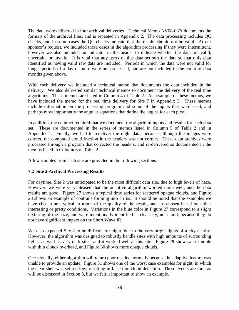
36

The data were delivered in four archival deliveries. Technical Memo AV08-037t documents the formats of the archival files, and is repeated in Appendix 2. The data processing includes QC checks, and in some cases the QC checks indicate that the results should not be valid. At our sponsor’s request, we included these cases in the algorithm processing if they were intermittent, however we also included an indicator in the header to indicate whether the data are valid, uncertain, or invalid. It is vital that any users of this data set sort the data so that only data identified as having valid raw data are included. Periods in which the data were not valid for longer periods of a day or more were not processed, and are not included in the count of data months given above. With each delivery we included a technical memo that documents the data included in the delivery. We also delivered similar technical memos to document the delivery of the real time algorithms. These memos are listed in Column 4 of Table 2. As a sample of these memos, we have included the memo for the real time delivery for Site 7 in Appendix 3. These memos include information on the processing program and some of the inputs that were used, and perhaps most importantly the angular equations that define the angles for each pixel. In addition, the contract required that we document the algorithm inputs and results for each data set. These are documented in the series of memos listed in Column 5 of Table 2 and in Appendix 1. Finally, we had to redeliver the night data, because although the images were correct, the computed cloud fraction in the headers was not correct. These data archives were processed through a program that corrected the headers, and re-delivered as documented in the memos listed in Column 6 of Table 2. A few samples from each site are provided in the following sections. 7.2 Site 2 Archival Processing Results For daytime, Site 2 was anticipated to be the most difficult data site, due to high levels of haze. However, we were very pleased that the adaptive algorithm worked quite well, and the data results are good. Figure 27 shows a typical time series for scattered opaque clouds, and Figure 28 shows an example of contrails forming into cirrus. It should be noted that the examples we have chosen are typical in terms of the quality of the result, and are chosen based on either interesting or pretty conditions. Variations in the blue color in Figure 27 correspond to a slight texturing of the haze, and were intentionally identified as clear sky, not cloud, because they do not have significant impact on the Short Wave IR. We also expected Site 2 to be difficult for night, due to the very bright lights of a city nearby. However, the algorithm was designed to robustly handle sites with high amounts of surrounding lights, as well as very dark sites, and it worked well at this site. Figure 29 shows an example with thin clouds overhead, and Figure 30 shows more opaque clouds. Occasionally, either algorithm will return poor results, normally because the adaptive feature was unable to provide an update. Figure 31 shows one of the worst case examples for night, in which the clear shell was set too low, resulting in false thin cloud detection. These events are rare, as will be discussed in Section 8, but we felt it important to show an example.

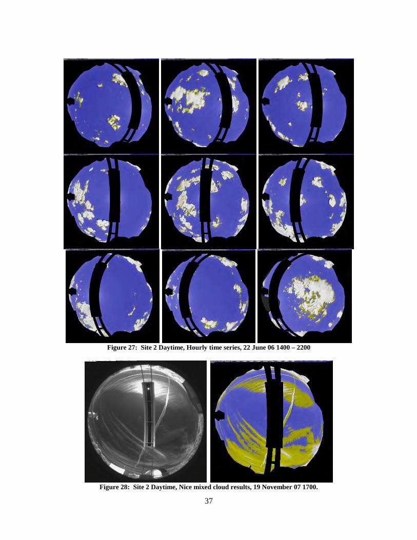
37

Figure 27: Site 2 Daytime, Hourly time series, 22 June 06 1400 – 2200

Figure 28: Site 2 Daytime, Nice mixed cloud results, 19 November 07 1700.

38

Figure 29: Raw Image and Cloud Algorithm Results for Site 2, 15 April 2008, 0620 GMT

Figure 30: Raw Image and Cloud Algorithm Results for Site 2, 16 April 2007, 0500 GMT

Figure 31: Raw Image and Cloud Algorithm Results for Site 2, 22 January 2008, 0600 GMT

39

7.3 Site 3 Archival Processing Results Site 3 was the last site installed, and had a shorter data base as a result. In addition, there were problems with both the cooler and the occultor that shortened the available data record. In spite of this, a reasonable data base was processed. Figure 32 shows a time series of day algorithm results at hourly intervals, and Figure 33 shows a nice case with both thin and opaque clouds and fine cloud structure. In Figure 33 we can also see some haze structure that was successfully identified as no cloud.

Figure 32: Site 3 Day, Hourly time series, 23 May 08 1400 – 2200.

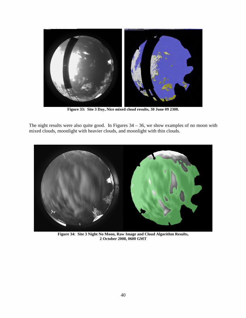
40

Figure 33: Site 3 Day, Nice mixed cloud results, 30 June 09 2300.

The night results were also quite good. In Figures 34 – 36, we show examples of no moon with mixed clouds, moonlight with heavier clouds, and moonlight with thin clouds.

Figure 34: Site 3 Night No Moon, Raw Image and Cloud Algorithm Results,

2 October 2008, 0600 GMT

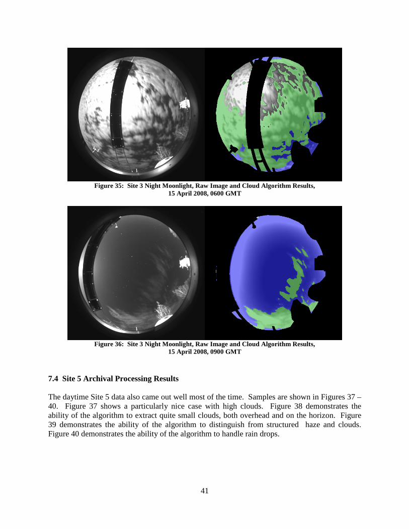
41

Figure 35: Site 3 Night Moonlight, Raw Image and Cloud Algorithm Results,

15 April 2008, 0600 GMT

Figure 36: Site 3 Night Moonlight, Raw Image and Cloud Algorithm Results,

15 April 2008, 0900 GMT 7.4 Site 5 Archival Processing Results The daytime Site 5 data also came out well most of the time. Samples are shown in Figures 37 – 40. Figure 37 shows a particularly nice case with high clouds. Figure 38 demonstrates the ability of the algorithm to extract quite small clouds, both overhead and on the horizon. Figure 39 demonstrates the ability of the algorithm to distinguish from structured haze and clouds. Figure 40 demonstrates the ability of the algorithm to handle rain drops.

42

Figure 37: Site 5 Day, Hourly time series, 10 April 09 1400 – 2200

The night algorithm at Site 5 was somewhat trickier, because part way through the first year, new lights showed up on the horizon, and caused considerable stray light. The algorithm was improved to handle this situation, and we were successful in handling most of the cases well, as illustrated in Figures 41 and 42.

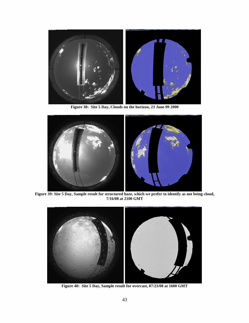
43

Figure 38: Site 5 Day, Clouds on the horizon, 23 June 09 2000

Figure 39: Site 5 Day, Sample result for structured haze, which we prefer to identify as not being cloud,

7/16/08 at 2100 GMT

Figure 40: Site 5 Day, Sample result for overcast, 07/23/08 at 1600 GMT

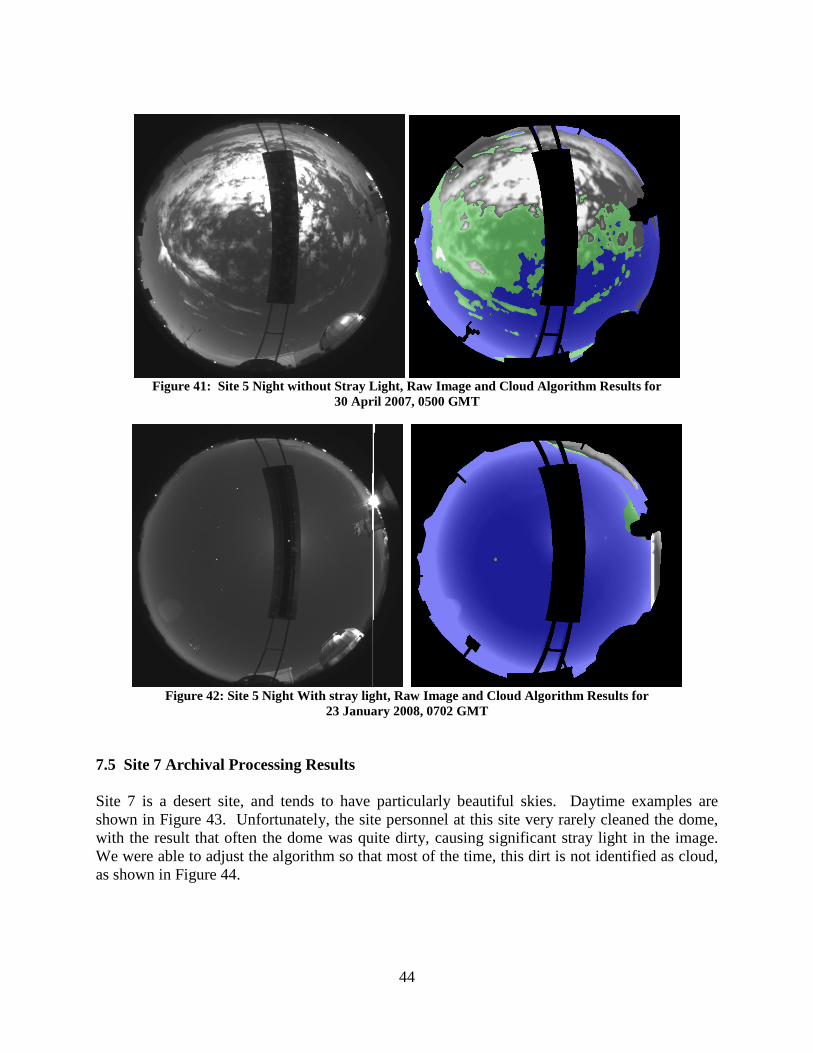
44

Figure 41: Site 5 Night without Stray Light, Raw Image and Cloud Algorithm Results for

30 April 2007, 0500 GMT

Figure 42: Site 5 Night With stray light, Raw Image and Cloud Algorithm Results for

23 January 2008, 0702 GMT 7.5 Site 7 Archival Processing Results Site 7 is a desert site, and tends to have particularly beautiful skies. Daytime examples are shown in Figure 43. Unfortunately, the site personnel at this site very rarely cleaned the dome, with the result that often the dome was quite dirty, causing significant stray light in the image. We were able to adjust the algorithm so that most of the time, this dirt is not identified as cloud, as shown in Figure 44.

45

Figure 43: Site 7 Day, Hourly time series, 18 February 09 1500 – 2300.

The night algorithm for Site 7 presented one special problem. Because this site is quite dark, additional upgrades to the algorithm were required to handle the Milky Way. This was actually required at some of the other sites also, but Site 7 required the largest adjustment. This adjustment was successful, and two sample results are shown in Figures 45 and 46. The Milky Way adjustment was written in such a way that it would work at all sites, including the bright sky sites.

46

Figure 44: Site 7 Day, Clear day with “dirt-effect”, 04 January 06 2000.

Figure 45: Site 7 Night, Raw Image and Cloud Algorithm Results for 13 April 2009, 0500 GMT

Figure 46: Site 7 Night, Raw Image and Cloud Algorithm Results, 18 February 2009, 1200GMT

47

8.0 TESTS OF ALGORITHM ACCURACY One of the more challenging aspects of this program is assessment of the accuracy of the algorithm. This work is documented in Memo AV09-099t, and summarized below. In general, we felt that by scanning large amounts of raw and processed data, we can find the main problems with the algorithm. As a result, our time is far better spent solving these problems than assessing the accuracy of the algorithm. However, some means to assess the accuracy of the algorithm can be very helpful. In general, we feel that both algorithms are quite good, although not perfect. The day algorithm has handled opaque clouds well for years, all the way down to the horizon, and under essentially all conditions we have encountered. The day thin cloud algorithm has worked very well except in heavy haze, when haze tends to be identified as thin cloud. In the last year, we have improved the thin cloud algorithm to include an adaptive feature that checks for haze amount and adjusts the algorithm. In this way, haze is not typically identified as thin clouds. Similarly, we feel that the night algorithm is quite good, although not perfect. For several years we used a contrast-based algorithm that provided good results but at lower resolution. In the last year we completed the high resolution version that works for both starlight and moonlight. It also includes an adaptive feature, so that as lighting levels change, the algorithm adjusts to it. We have not developed a sunrise/set algorithm at this time. Looking at the raw data, it appears that a sunrise/set algorithm should be possible but not trivial, and it never rose to the top of the priority pile. One reason we believe that these algorithms are good is that if one looks at either a 1-minute time series for a period of a few hours, or looks at hourly data for a period of a month or more, most of the cases look almost perfect. There will be a few cases where the results are not good in portions of the sky, and these are generally associated with a thin cloud field that was mostly missed. This generally happens when the adaptive algorithm is unable to provide a good update. Some of this loss of thin cloud is legitimate: we do not expect all thin clouds to be detected, because there is a threshold for the thin cloud identification. That is, it is acceptable to our sponsors that clouds with more than 1dB fade (or some other threshold) are identified as thin cloud, and clouds with less than 1 dB be identified as no cloud. As a result, thin clouds that we can see visually in the image may or may not be identified, because they may or may not be more attenuating than our threshold. The cloud algorithms generally do well if we’ve had an opportunity to update the algorithm inputs within the last year or two. For the night algorithm, it is also important that the alignment has not been changed within the data processing interval, because it needs to find the stars. Beginning about 2005, we worked on providing a more quantitative assessment of the accuracy of the algorithms, partly so that we could assess whether our algorithms were improving. Although this was never as high priority as actually improving the algorithms, we have assessed the cloud algorithm quantitatively in a few ways over the years. This section provides an overview of these results, as well as the most recent results using a blind test.

48

8.1 Program SORCloudAssess Our first significant attempt to provide a quantitative assessment of the accuracy of the cloud algorithms was done with the program SORCloudAssess. In 2005, we were being encouraged to find some method to assess the accuracy. Our sponsors had tried to compare the WSI results with a lidar, but there were too many problems with pointing, with the lidar accuracy, and perhaps with manpower, for this to be practical. One problem with a lidar comparison is that the lidar may identify extremely thin clouds (below our threshold) at lower altitudes, and yet miss significant clouds at higher altitudes, depending on the type of lidar or ceilometer used. In response, we wrote a program that would allow us to show the raw image in a display beside the processed image, highlight a few Regions of Interest (ROI), and have a user make a visual assessment of whether the answers appeared to be correct or incorrect. The typical display, with arrows to show the locations of the ROI’s, is shown in Figure 47.

Figure 47: Slide from Dec 05 talk showing the format of the SORCloudAssess Display

The program is documented in Technical Note 27226. The initial day algorithm sample results are also in Tech Note 272, and shown in Figure 48. These results were for a test set from the SOR site. Figure 48 shows the overall fraction assessed to have correct results, for 3401 Regions of Interest (ROI), from 310 images acquired during the July and August 2005 period.

49

Figure 48: Fraction of correct answers, in percent, for each ROI for SOR Day Test Bed Processing

This analysis showed that at least within the limits of the analyst’s ability to assess the raw images, the algorithm is quite accurate overhead (99%), and less accurate on the horizons (about 95%). Soon after this, we also processed a daytime set from a very test hazy test site. At that time, we did not have the adaptive algorithm (for either the SOR processing or the test site processing), but we found that if we were allowed to make one adjustment similar to the anticipated adaptive adjustment, we got quite good results. The results are summarized for both sites in Table 3, and a figure similar to Figure 48 is shown in Tech Note 27226. The night was not quite so straightforward to evaluate, because at that time the night algorithm was not a high resolution algorithm, i.e. there was not a specific result for each pixel, but only for each 5˚ zenith by 15˚ azimuthal cell. As explained in Tech Note 27226, we assessed the line of sight, as well as the region of sight, using the methods documented in Memo AV05-037t. The results for assessing the region of sight are shown in Figure 49, and the results for both methods of assessment are shown in Table 4. We did not process night data from the hazy test site.

99.0

97.6

98.6

97.7

97.7

97.9

96.5

94.8

94.9

97.8

98.3

50

Table 3

Summary of Estimated Accuracy for the Day Cloud Algorithm Using SORCloudAssess

For the SOR and Hazy Test Site Test Bed Data Sets

Region SOR Results Haze Results Overall 98.4% 98.1% Zenith 99.5% 97.5%

Horizons 98.5% 98.8% 90% Correct? 96.7% 96.7%

Figure 49: Fraction of correct answers, in percent, for each ROI for SOR Night Test Bed for Region of Sight We were encouraged by these results. When one is working hard to make the algorithm as good as possible, it’s easy to notice only the bad results. However, it appeared that the day algorithm was accurate to about 98%, and the night algorithm using the region of sight was accurate to about 95%. This was before we had developed the latest versions of the algorithms, and it was when we judged any miss of a thin cloud as an error. It was not a blind test, but a major effort

97.9

98.4

97.9

96.8

96.3

98.9

99.5

99.5

95.7

87.2

81.4

51

was made to be honest and not introduce bias. Also, in making the assessments, if the sky condition was not obvious from the raw image, we could zoom it, enhance it, and bring in the ratio image to further assess it. The assessments were all done by the primary author, who had years of experience looking the actual sky in the field and the concurrent image.

Table 4 Summary of Estimated Accuracy for the Night Cloud Algorithm

Using SORCloudAssess For the SOR Test Bed Data Set

Region LOS Results ROS Results Overall 87.7% 95.5% Zenith 93.1% 97.9%

Eastern Horizon 87.8% 99.5% Western Horizon 70.2% 81.4%

70% Correct? 95.2% In September 2006, we presented the high resolution night algorithm that handled starlight well, but did not yet handle moonlight. At that time, we evaluated some of the data using SORCloudAssess. Figure 50 shows the results for no moon. We were very pleased with these results also. The sponsor no longer cared so much about the horizons, and if the horizons were not counted, we estimated about 95.7% accuracy with this method. If the horizons are included, then the estimate was about 94.3%. For moonlight, the results were 77%, i.e. not nearly as good, as we expected, since the moonlight algorithm was yet to be developed. These results were presented in Technical Note 27327, although Figure 35 of that report has an error, and is corrected in Memo AV06-033t and in Figure 50. Once the moonlight algorithm was completed, we evaluated data for Site 5. The estimated accuracy for both moonlight and starlight conditions combined was 93.1% for the whole sky, and 95.3% for angles above 60 degrees. The results are shown in Figure 51. For the whole sky, the starlight and moonlight results were very similar, being 92.4% for moonlight and 93.8% for no moon. The algorithms were improved slightly before we did the final processing, but we didn’t have the time to go back and reassess the accuracy.

52

99.2

95.9

98.3

94.2

58.3

97.5

88.4

92.6

88.1% 99.0% 96.7

Figure 50: Site 2 Night results for no moon, 3 May – 27 June 2006

Figure 51: Site 5 Night results for all conditions, with hi resl algorithm that handles moon and no moon

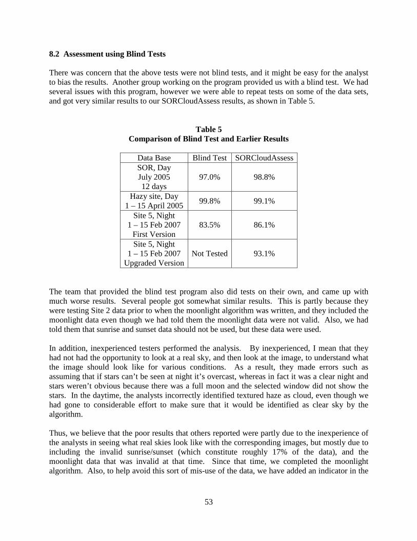
53

8.2 Assessment using Blind Tests There was concern that the above tests were not blind tests, and it might be easy for the analyst to bias the results. Another group working on the program provided us with a blind test. We had several issues with this program, however we were able to repeat tests on some of the data sets, and got very similar results to our SORCloudAssess results, as shown in Table 5.

Table 5 Comparison of Blind Test and Earlier Results

Data Base Blind Test SORCloudAssess SOR, Day July 2005 12 days

97.0% 98.8%

Hazy site, Day 1 – 15 April 2005 99.8% 99.1%

Site 5, Night 1 – 15 Feb 2007

First Version 83.5% 86.1%

Site 5, Night 1 – 15 Feb 2007

Upgraded Version Not Tested 93.1%

The team that provided the blind test program also did tests on their own, and came up with much worse results. Several people got somewhat similar results. This is partly because they were testing Site 2 data prior to when the moonlight algorithm was written, and they included the moonlight data even though we had told them the moonlight data were not valid. Also, we had told them that sunrise and sunset data should not be used, but these data were used. In addition, inexperienced testers performed the analysis. By inexperienced, I mean that they had not had the opportunity to look at a real sky, and then look at the image, to understand what the image should look like for various conditions. As a result, they made errors such as assuming that if stars can’t be seen at night it’s overcast, whereas in fact it was a clear night and stars weren’t obvious because there was a full moon and the selected window did not show the stars. In the daytime, the analysts incorrectly identified textured haze as cloud, even though we had gone to considerable effort to make sure that it would be identified as clear sky by the algorithm. Thus, we believe that the poor results that others reported were partly due to the inexperience of the analysts in seeing what real skies look like with the corresponding images, but mostly due to including the invalid sunrise/sunset (which constitute roughly 17% of the data), and the moonlight data that was invalid at that time. Since that time, we completed the moonlight algorithm. Also, to help avoid this sort of mis-use of the data, we have added an indicator in the

54

header to indicate if the algorithm result is expected to be valid or not, and we also do not process the sunrise and sunset data. More recently, we also developed new programs, AssessRaw and AssessProcCloud, that provide a blind test, but avoid the problems we were concerned about with the other blind tests. Program AssessRaw was designed to allow the analyst to indicate whether the ROI’s in a raw image were opaque cloud, thin cloud, no cloud, uncertain, or no data. The program is documented in Memo AV08-042t, and AV09-099t. The program saves the analyst’s results in a file. In this way, we only have to assess the raw data once, and can easily test multiple versions of processed algorithm results. The saved file also includes the solar and lunar zenith angle, so that we can more easily evaluate the conditions under which the algorithm does well and poorly. The program also allows the user to use any of the V++ image processing program features, including zooming, re-windowing, and so on. Also, this program uses an ROI of 9 x 9 pixels, so it’s easier to see what’s going on within the ROI. (Later, it might be better to use 3 x 3 regions however.) Program AssessProcCloud is documented in Memo AV08-043t and AV09-099t. This program takes a data set of processed cloud algorithm results, and compares it with the tables output from AssessRaw to determine how often the analyst and the algorithm agreed. The statistics are presented such that the analyst can either look separately at the results for opaque and thin cloud, or can look at the net result. By the time these programs were written, the sponsors were convinced that the algorithms did reasonably well, from looking at samples, time lapse series, and the statistics shown in Table 5. As a result, their priority was to get as much data processed as possible, so we limited the amount of analysis done with these programs. We were able to analyze small samples of data processed with the new algorithms. The biggest challenge with processing these tests was to decide what to call “uncertain”. Any test like this should ideally test the accuracy of the algorithm, not the human error associated with the test. Also, we decided to take into account the fact that the sponsors feel that a non-zero fade threshold thin clouds is reasonable. (As discussed in Section 6, if the thin clouds are only detected if the fade is 1dB or more, that is a good result.) The rules we used for identifying ROI’s as uncertain were the following: a) For the reasons discussed above, the analyst identified areas where there are very thin clouds as uncertain, if it was not easy to tell if they are more or less thin than the thresholds. b) In holes or near edges of Cumulus clouds, there is often cloud debris within these regions. This doesn’t always happen, but it does sometimes. This effect appears to be real, and we have observed it visually from airplanes. We can't always tell visually from the raw image if there's cloud debris in the small holes and near cloud edges. Also, often it’s a challenge to tell if there are higher thin layers that could be detected in the small holes. So we called these regions uncertain.

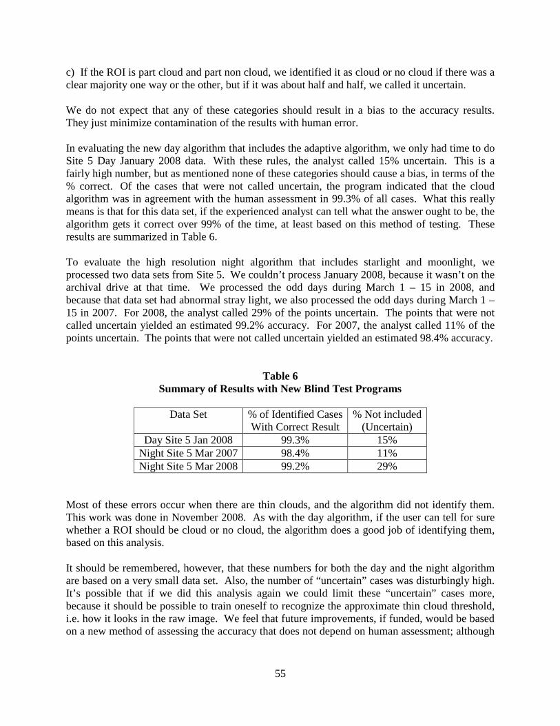
55

c) If the ROI is part cloud and part non cloud, we identified it as cloud or no cloud if there was a clear majority one way or the other, but if it was about half and half, we called it uncertain. We do not expect that any of these categories should result in a bias to the accuracy results. They just minimize contamination of the results with human error. In evaluating the new day algorithm that includes the adaptive algorithm, we only had time to do Site 5 Day January 2008 data. With these rules, the analyst called 15% uncertain. This is a fairly high number, but as mentioned none of these categories should cause a bias, in terms of the % correct. Of the cases that were not called uncertain, the program indicated that the cloud algorithm was in agreement with the human assessment in 99.3% of all cases. What this really means is that for this data set, if the experienced analyst can tell what the answer ought to be, the algorithm gets it correct over 99% of the time, at least based on this method of testing. These results are summarized in Table 6. To evaluate the high resolution night algorithm that includes starlight and moonlight, we processed two data sets from Site 5. We couldn’t process January 2008, because it wasn’t on the archival drive at that time. We processed the odd days during March 1 – 15 in 2008, and because that data set had abnormal stray light, we also processed the odd days during March 1 – 15 in 2007. For 2008, the analyst called 29% of the points uncertain. The points that were not called uncertain yielded an estimated 99.2% accuracy. For 2007, the analyst called 11% of the points uncertain. The points that were not called uncertain yielded an estimated 98.4% accuracy.

Table 6 Summary of Results with New Blind Test Programs

Data Set % of Identified Cases

With Correct Result % Not included

(Uncertain) Day Site 5 Jan 2008 99.3% 15%

Night Site 5 Mar 2007 98.4% 11% Night Site 5 Mar 2008 99.2% 29%

Most of these errors occur when there are thin clouds, and the algorithm did not identify them. This work was done in November 2008. As with the day algorithm, if the user can tell for sure whether a ROI should be cloud or no cloud, the algorithm does a good job of identifying them, based on this analysis. It should be remembered, however, that these numbers for both the day and the night algorithm are based on a very small data set. Also, the number of “uncertain” cases was disturbingly high. It’s possible that if we did this analysis again we could limit these “uncertain” cases more, because it should be possible to train oneself to recognize the approximate thin cloud threshold, i.e. how it looks in the raw image. We feel that future improvements, if funded, would be based on a new method of assessing the accuracy that does not depend on human assessment; although

56

human visual assessment will always be a useful backup, and a convenient way to assess the different data sites and periods.

57

9.0 RECOMMENDED FURTHER DEVELOPMENTS As noted earlier, originally this program was intended to be a five-year program. However, due to changing priorities at higher levels, the program that this contract was a part of was cancelled early in this period. Fiscally, we received the funding from the first year and a small fraction of the second year. In calendar time, we were able to extend the period to 1 year and 11 months. Although we were very pleased to get the instruments fielded, and to process the full data archival for the 3 primary sites, there was much work that remained that would benefit the use of Whole Sky Imagers in documenting the environment and supporting applications and research. This section gives a brief overview of the recommended next steps. 9.1 Hardware Upgrades The Day/Night WSI systems are fairly old, having been built in the mid- to late-nineties. We feel that if a major program were planned using this type of system, it would be appropriate to develop a design upgrade. As discussed in Section 3, the subassembly that had the most failures was the solar/lunar occultor. This is a fairly large device, out in the open. It is complex, because in order to handle both sun and moon, it must have two degrees of freedom, i.e. rotate east-to-west and move north-to-south, or have similar motion. Also, it must be fairly large, because we must shade the whole dome for optimum data quality, and that means that the shade must be reasonably far from the optics so that the blocked angle is not unreasonably large. Prior to this contract, we had created a design mock-up for the next generation occultor, and during this contract we began work on the design drawings. This work was halted when we had to curtail the spending rate about 10 months into the program. This new design included an arc, similar to the existing arc, but it was mounted on a rotating bearing to provide the second degree of freedom. We felt this design would be much more robust, as it avoids having to use the trolley. The design also would have included upgrades to avoid the mechanical problems that sometimes affected the arc drive. Another major upgrade would be nearly eliminating the Accessory Control Panels. These ACP units were designed to allow either manual or computer control of all the components. At this point, it would be far less costly and more robust to use modern techniques to connect directly to the computer, and use manual or automated computer control and readout. Other ACP simplifications were envisioned; for example, by using encoders rather than potentiometers to monitor the occultor position, then the electronic design became much simpler. There were a number of other upgrades and simplifications that we had in mind, that are beyond the scope of this report to discuss.

58

9.2 Adding Optical Fade Parameters As discussed in Section 6, we developed an automated product to provide the earth-to-space beam transmittance at night. Additional products could readily be developed to provide the transmittance corrected for the aerosol amount, and to compute the optical fade through the clouds. In addition, as discussed in Memo AV08-053t, we developed concepts and methods to determine optical fade in the daytime, but did not have the time to do this work. This could be a very valuable data product. 9.3 Further Algorithm Development and Evaluation Although the algorithms are generally quite good, there are times when the results are not good. We would have liked to further evaluate these cases. For example, in the daytime, when the results are bad, it’s generally because the program was unable to find an adaptive correction along the beta line. If the logic were expanded to allow the algorithm to try to identify an adaptive correction in broader areas of the image, this might take care of this issue. Another logical next step is to develop the sunrise/sunset algorithm. We evaluated the raw data, and felt that this should be feasible, although it may be more complicated than the day algorithm. More importantly, we would like to evaluate what the optical fade is that’s associated with the thin cloud and opaque cloud thresholds, and evaluate how consistent it is. We would expect the threshold to be approximately associated with a given level of fade, but do not expect the relationship to be precise. Determination of the average, mean and STD values of optical fade associated with the thresholds would be very valuable. 9.4 Analysis of the Data Base As part of this contract, we have created a large data base of cloud images, taken every 1 minute in the daytime and 2 minutes at night, for at least 17 months (up to 41 months) at each of 4 sites. Also, we have developed and polished the algorithms to make additional data processing of prior data acquired with the WSI systems much easier. These data should be very valuable for a number of studies, such as evaluation of the accuracy of satellite data (how often can they detect the thin clouds that the WSI detects). It would be useful to extract cloud free line of sight (CFLS) statistics, as well as related statistics such as CFLOS persistence. We have previously extracted these statistics for other more limited data bases37. Also, at one point we had started doing analysis of forecasting of CFLOS, as discussed in Memo AV05-036t. In general, we feel we made tremendous progress on this contract, in terms of development of algorithms and processing of data archives. We appreciate having had this opportunity.

59

10.0 DISCUSSION OF CONTRACT REQUIREMENTS At this time, the requirements of the Contract Data Requirements List (CDRL) and of the Statement of Work (SOW) have been completed to the best of our knowledge. Section 10.1 provides a brief overview of the CDRL requirements. It should be noted that since we received only 24% of the original budgeted amount, we had to compromise in some cases on items such as formats of CDRL items. In all cases, these compromises were provided many months before the close of the contract, and we received no objections from the sponsors. Section 10.2 discusses the SOW items that must be discussed in the report according to CDRL A001, and Section 10.3 discusses the other SOW items in the technical requirements list. 10.1 Overview of CDRL Requirements CDRL A001 is a requirement to complete a final report. This report constitutes that report. As a part of this report, we are required to discuss part of the SOW. This will be discussed below in Section 10.2. CDRL A002 requires presentations at meetings. Presentations were made at meetings in May 2008, September 2008, and October 2008. Letters of Transmittal were sent to document these presentations, as well as any meetings for which no presentations were made, due to priorities from the sponsors. No presentations were made in 2009, because meetings were cancelled due to the funding restrictions. Letters A002.1 through A002.7 document meeting this requirement. CDRL A003 requires a software user manual. Due to the funding limitations, we delivered this information in the form technical memos documenting the use of the software and any changes to the software, rather than the format indicated in the CDRL list. This provided the sponsors with the information they needed, but at lower cost. These memos are listed in Appendix 1. Letters A003.1 through A003.9 document meeting this requirement. CDRL A004 requires “Test/Inspection Reports”, which are actually documentation of the results of setting up the algorithm inputs. Due to the funding limitations, we delivered this information in the form of technical memos documenting the algorithm input extraction and results rather than the format indicated in the CDRL list. This provided the sponsors with the information they needed, but at lower cost. These memos are listed in Appendix 1. Letters A004.1 through A004.11 document meeting this requirement. CDRL A005 requires monthly status reports. These were delivered every month, in the format required by the CDRL. Letters A005.1 through A005.16 document meeting this requirement. CDRL A006 requires technical management and work plans. These were delivered in 2008, as documented in Letter A006.1 and A006.2. CDRL A007 requires delivery of the computer software product end items. These were delivered in 2009, as documented in Letter A007.1.

60

CDRL A008 requires delivery of an operations manual. Due to the funding limitation, it was not possible to create a formal manuscript in the format specified in the original CDRL. However, we delivered technical memos documenting the use and repair of the instrument throughout the program, and toward the end of the program we provided another technical memo that referenced all of these memos, as suggested by the sponsors. This work was documented in Letter A008.1. 10.2 Discussion of the SOW Sections 3.4 through 3.7 The CDRL for Item A001 (for the final report) requires that we discuss the SOW Items 3.4 through 3.7. SOW Item 3.4 is stated as follows. Perform calibration of the five fielded instruments and quality control of data acquired by the WSI and the performance of the cloud decision algorithm. Calibration consists of two parts 1) clear sky background determination in order to accurately detect clouds in the daytime and 2) geocal within two (2) degrees to ensure instrument alignment has not drifted in order to accurately detect clouds at night The government will supply raw camera imagery and/or processed cloud masks from the WSIs as required to accomplish this task. Upon receipt of the data, the contractor shall, within 30 days, complete the calibration analysis, update the control software with the calibration files, supply the updated software to the government, and install the updated software in the fielded WSIs. At a minimum, calibrations shall be evaluated twice per year for each instrument and updated as necessary to provide the highest quality cloud masks. The contractor shall request, at least quarterly, data from the WSIs to perform quality control of the cloud mask results and system performance. The contractor shall maintain the cloud decision algorithm code used to create the cloud masks and provide documentation of the code to the government. The clear sky background extraction, and the geo cal extraction, as well as all the other required model extractions, were completed on all systems. As the inputs were extracted, they were put in the field, and also archival data were processed. This work is discussed in Section 7 and in numerous memos listed in Appendix 1. At the time the program closed, 4 of the 5 systems had been fielded, so these comments only apply to these 4 systems. SOW Item 3.5 is stated as follows. Evaluate WSI capabilities. Areas to be evaluated include, but are not limited to: 1) day and night cloud decision algorithm performance – for this task, the government may provide “truth” data to use for extraction, 2) applicability of data to cloud forecasting problems, 3) capability to extract atmospheric transmission both day and night, 4) dynamic clear sky background calibrations; 5) operation in stressing conditions such as high light levels at night, twilight, and heavy haze, and 6) any other area that both the contractor and government feel to be beneficial to government programs.

61

Regarding the algorithm performance, we evaluated each site in some detail, as reported in the memos listed in Appendix 1. We also did some development of assessment methods, and further assessed the results, as discussed in Section 8. We feel that the day algorithm is accurate to within about 98% or better and the night algorithm within about 95 % or better. Regarding item 2, applicability to the cloud forecasting problems, this was not funded. Regarding item 3, ability to extract atmospheric transmission both day and night, this capability was completed for night, as documented in Section 6, but the capability for day was not funded. Regarding dynamic clear sky background calibrations, this feature was completed in both the day and night algorithm, as discussed in Sections 4 and 5. Regarding operation in stressing conditions, Site 2 had high light levels at night, and the results were very good, as discussed in Section 7. The development for twilight was not funded. And the development for heavy haze was completed. Site 2 had heavy haze, and the results were very good, as discussed in Section 7. SOW Item 3.6 is stated as follows. Implement system upgrades resulting from work accomplished under item 3.5 as coordinated with the government program manager. The quantity and delivery instructions will be set forth in contract modification. This contract modification was not funded. SOR Item 3.7 is stated as follows. Build and deploy additional WSIs at locations to be determined by the government, providing training to on-site caretakers if required. The quantity and delivery instructions will be set forth in contract modification. This contract modification was not funded. 10.3 Discussion of the SOW Sections 3.1 through 3.3, 3.8, and 3.9 Although discussion of the other SOW technical requirements is not required in the CDRLs, we will provide a brief overview of these requirements as well. SOW Item 3.1 requires that 5 sites be supported, and that system failures be repaired in a timely manner. At the time the program ended, we had accomplished the fielding of 4 sites. The program was curtailed before a fifth site location was selected by the sponsors. When we first bid the proposal, we had included in the budget funding for two hardware people, so that we could repair systems in a timely way. During the negotiations, we were requested to decrease the budget to have only one hardware person, with the understanding that repairs would not be quite as fast. In spite of this, we were generally able to complete repairs in a timely way. The detailed repair record is discussed in Memo AV09-104t. SOW Item 3.2 requires that a cloud decision algorithm capable of achieving 80% accuracy be provided. The new day and night algorithms are discussed in Sections 4 and 5, and their accuracy is illustrated in Section 7. Tests of the accuracy are discussed in Section 9. Although

62

none of the tests is perfect, we believe that the night algorithm is accurate to 95% or better, and the day algorithm is accurate to 98% or better. SOW Item 3.3 basically required us to get spare parts operational at MPL, and to monitor the instrument operational statistics. We got a full up spare system running in 2008, and improved QC programs to enable convenient monitoring. Sometimes the QC effort was compromised because the SOR team either lost connectivity with the instruments, or lacked the time to pull the QC files. When we had access to the files however, we monitored them promptly. Results were reported on a monthly basis when the QC files had been provided by the SOR team. SOW Items 3.4 through 3.7 are discussed in Section 10.2, as their discussion is required by the CDRL. SOW Item 3.8 required evaluation of new wavelength imaging benefits. Most of the interest was in evaluating the pros and cons of using an IR system. This work was completed under the previous contract (after the Request for Proposal was written, but before this current contract was funded). It was reported to the sponsors in January 2008, and also in the previous contract report, Technical Note 27428. SOW Item 3.9 was an open task to enable the sponsors to provide new funding for additional tasks as required. This contract modification was not funded. We believe we have met all funded contract requirements as stated in the SOW or CDRLs at this time.

63

11.0 SUMMARY OF THE REPORT In this report, we have provided an overview of the Whole Sky Imager system and its data base. A summary of the work is provided in Section 1. In the body of the report, we have provided overviews of both the day and the night algorithm, and discussed in more detail the final upgrades that make these algorithms mature. New developments that are discussed include the further development of the night transmittance product, and the further development of algorithm accuracy analysis methods. We have discussed the processing of the full data archive, and provided many examples of results. Finally, we have discussed the contract requirements listed in the CDRLS. As stated in that section, we believe we have completed all funded contract requirements with the completion of this report.

64

12.0 ACKNOWLEDGEMENTS We would like to express our appreciation to the personnel of Starfire Optical Range and their contractors from Boeing. Capt. Douglas MacPherson and Lt. Lyrica Phelps were our contract monitors, and were very helpful and supportive. Marjorie Shoemake and Darielle Dexheimer worked with us regularly providing data, QC files, and helping diagnose hardware problems. They were always a pleasure to work with. Ann Slavin has worked with us for many years on this project, and has always been tremendously helpful. The SOR team is always a pleasure to work with. We feel this WSI work is valuable, and very much appreciate having had the chance to advance the state of the art, as well as meet our sponsor’s specific needs.

65

13.0 REFERENCES 1. Johnson, R. W., Koehler, T. L., and Shields, J. E., “A Multi-Station Set of Whole Sky Imagers and A Preliminary Assessment of the Emerging Data Base”, Proc. of the Cloud Impacts on DOD Operations and Systems, 1988 Workshop pp. 159 – 162 1988. 2. Johnson, R. W., Hering, W. S., and Shields, J. E., Automated Visibility and Cloud Cover Measurements with a Solid State Imaging System, University of California, San Diego, Scripps Institution of Oceanography, Marine Physical Laboratory, SIO 89-7, GL-TR-89-0061, NTIS No. ADA216906, 1989. 3. Shields, J. E., Johnson, R. W., and Koehler, T. L., “Automated Whole Sky Imaging Systems for Cloud Field Assessment”, Fourth Symposium on Global Change Studies, American Meteorological Society, 1993. 4. Shields, J. E., Johnson, R. W., Karr, M. E., and Wertz, J. L., “Automated Day/Night Whole Sky Imagers for Field Assessment of Cloud Cover Distributions and Radiance Distributions”, Tenth Symposium on Meteorological Observations and Instrumentation, American Meteorological Society, pp165 – 170, 1998. 5. Shields, J. E., Johnson, R. W., Karr, M. E., Burden, A. R., and Baker, J. G., “Whole Sky Imagers for Real-time Cloud Assessment, Cloud Free Line of Sight Determinations and Potential Tactical Applications”, The Battlespace Atmospheric and Cloud Impacts on Military Operations (BACIMO) Conference, Monterey, CA. http://www.nrlmry.navy.mil/bacimo.html, 2003. 6. Duntley, S. Q., Johnson, R. W., and Gordon, J. I., Airborne Measurements of Optical Atmospheric Properties in Southern Illinois, University of California, San Diego, Scripps Institution of Oceanography, Visibility Laboratory, SIO Ref. 73-24, AFCRL- TR-0422, NTIS No. AD-774-597, 1973. 7. Duntley, S. Q., Johnson, R. W., and Gordon, J. I., Airborne Measurements of Optical Atmospheric Properties in Northern Germany, University of California, San Diego, Scripps Institution of Oceanography, Visibility Laboratory, SIO Ref. 76-17, AFGL- TR-0188, NTIS No. ADA-035-571, 1976. 8. Johnson, R. W., Hering, W. S., Gordon, J. I., Fitch, B. W., and Shields, J. E., Preliminary Analysis and Modeling Based Upon Project OPAQUE Profile and Surface Data, University of California, San Diego, Scripps Institution of Oceanography, Visibility Laboratory, SIO Ref. 80-5, AFGL- TR-0285, NTIS No. ADB-052-1721, 1980. 9. Shields, J. E., Koehler, T. L., and Johnson, R. W., “Whole Sky Imager”, Proceedings of the Cloud Impacts on DOD Operations and Systems, 1989/90 Conference, 1990. 10. Koehler, T. L., Johnson, R. W. and Shields, J. E., “Status of the Whole Sky Imager Database”, Proceedings of the Cloud Impacts on DOD Operations and Systems, 1991 Conference, 1991. 11. Johnson, R. W., Shields, J. E. and Koehler, T. L., Analysis and Interpretation of Simultaneous Multi-Station Whole Sky Imagery, University of California, San Diego, Scripps Institution of Oceanography, Marine Physical Laboratory, SIO 91-33, PL-91-2214, NTIS No. ADA253658, 1991. 12. Shields, J. E., Burden, A. R., Johnson, R. W., Karr, M. E., and Baker, J. G., “New cloud free line of sight statistics measured with digital Whole Sky Imagers”, International Symposium on Optical Science and Technology, SPIE the International Society for Optical Engineering, August 2005. 13. K. M. Watson, Shields, J. E., Johnson, R. W., Koehler, T. L., and Karr, M. E., Upgrade of the LIMDAS Day/Night Whole Sky Imager, Final Report to the Office of Naval Research Contract N00014-89-D-0142 (DO #28), University of California, San Diego, Scripps Institution of Oceanography, Marine Physical Laboratory, MPL-U-30/93, NTIS No. ADA265871, 1993. 14. Shields, J. E., Johnson, R. W., and Karr, M. E., Upgrading the Day/Night Whole Sky Imager from Manual/Interactive to Full Automatic Control, Final Report to the Office of Naval Research Contract N00014-89-D-

66

0142 (DO #18), University of California, San Diego, Scripps Institution of Oceanography, Marine Physical Laboratory, MPL-U-140/94, NTIS No. ADA292296, 1994. 15. Shields, J. E., Johnson, R. W., Karr, M. E., R. A. Weymouth, and D. S. Sauer, Delivery and Development of a Day/Night Whole Sky Imager with Enhanced Angular Alignment for Full 24 Hour Cloud Distribution Assessment, Final Report to the Office of Naval Research Contract N00014-93-D-0141 (DO #11), University of California, San Diego, Scripps Institution of Oceanography, Marine Physical Laboratory, MPL-U-8-97, NTIS No. ADA333269, 1997. 16. Shields, J. E., Karr, M. E., and Johnson, R. W., Service Support for the Phillips Laboratory Whole Sky Image, Final Report to the Office of Naval Research Contract N00014-96-D-0065 (DO #3), University of California, San Diego, Scripps Institution of Oceanography, Marine Physical Laboratory, MPL-U-10-97, NTIS No. ADA333283, 1997. 17. Shields, J. E., Johnson, R. W., and Karr, M. E., Continued Upgrade of the LIMDAS Day/Night Whole Sky Imager for Night Cloud Monitoring, Final Report to the Office of Naval Research Contract N00014-93-D-0141 (DO #1), University of California, San Diego, Scripps Institution of Oceanography, Marine Physical Laboratory, MPL-U-1-98, 1998. 18. Shields, J. E., Karr, M. E., Burden, A. R., Johnson, R. W., and J. B. Baker, Analytic Support of the Phillips Lab Whole Sky Imager1997-2001, Final Report to the Office of Naval Research Contract N00014-97-C-0385, University of California, San Diego, Scripps Institution of Oceanography, Marine Physical Laboratory, ADA425323, MPL AOG TN 257, 2002. 19. Shields, J. E., Karr, M. E., Tooman, T. P., Sowle, D. H., and Moore, S. T., “The Whole Sky Imager – A Year of Progress”, Proceedings of the Eighth Atmospheric Radiation Measurement (ARM) Science Team Meeting, 1998. 20. Shields, J. E., Karr, M. E., Burden, A. R., Johnson, R. W., and J. B. Baker, Analysis and Measurement of Cloud Free Line of Sight and Related Cloud Statistical Behavior, Final Report to the Office of Naval Research Contract N00014-89-D-0142 (DO #2), University of California, San Diego, Scripps Institution of Oceanography, Marine Physical Laboratory, ADA425400, MPL AOG TN 262, 2003. 21. Shields, J. E., Karr, M. E., Burden, A. R., Johnson, R. W., and J. B. Baker, Project Report for Providing Two Day/Night Whole Sky Imagers and Related Development Work for Starfire Optical Range, Final Report to the Office of Naval Research Contract N00014-97-D-0350 (DO #6), University of California, San Diego, Scripps Institution of Oceanography, Marine Physical Laboratory, ADA not assigned, MPL AOG TN 265, 2004. 22. Shields, J. E., Burden, A. R., Karr, M. E., Johnson, R. W., and J. B. Baker, Development of Techniques for Determination of Nighttime Atmospheric Transmittance and Related Analytic Support for the Whole Sky Imager, Final Report to the Office of Naval Research Contract N00014-01-D-0043 (DO #5), University of California, San Diego, Scripps Institution of Oceanography, Marine Physical Laboratory, ADA not assigned, MPL AOG TN 263, 2004. 23. Shields, J. E., Burden, A. R., Johnson, R. W., Karr, M. E., and Baker, J. G., “Measurement and Evaluation of Cloud Free Line of Sight with Digital Whole Sky Imagers”, The Battlespace Atmospheric and Cloud Impacts on Military Operations (BACIMO) Conference, Monterey, CA. http://www.nrlmry.navy.mil/bacimo.html, 2005. 24. Shields, J. E., Burden, A. R., Johnson, R. W., Karr, M. E., and Baker, J. G., Cloud Free Line of Sight Probabilities and Persistence Probabilities from Whole Sky Imager Data, University of California, San Diego, Scripps Institution of Oceanography, Marine Physical Laboratory, MPL AOG TN 266, 2006. 25. Shields, J. E., Karr, M. E., Burden, A. R., Johnson, R. W., and Hodgkiss, W. S., Enhancement of Near-Real-Time Cloud Analysis and Related Analytic Support for Whole Sky Imagers, Final Report for ONR Contract N00014-01-D-0043 DO #4, Marine Physical Laboratory, Scripps Institution of Oceanography, University of California San Diego, Technical Note 271, May 2007.

67

26. Shields, J. E., Karr, M. E., Burden, A. R., Johnson, R. W., and Hodgkiss, W. S., Whole Sky Imaging of Clouds in the Visible and IR for Starfire Optical Range, Final Report for ONR Contract N00014-01-D-0043 DO #11, Marine Physical Laboratory, Scripps Institution of Oceanography, University of California San Diego, Technical Note 272, July 2007. 27. Shields, J. E., Karr, M. E., Burden, A. R., Johnson, R. W., and Hodgkiss, W. S., Continuing Support of Cloud Free Line of Sight Determination including Whole Sky Imaging of Clouds, Final Report for ONR Contract N00014-01-D-0043 DO #13, Marine Physical Laboratory, Scripps Institution of Oceanography, University of California San Diego, Technical Note 273, November 2007. 28. Shields, J. E., Karr, M. E., Burden, A. R., Johnson, R. W., Mikuls, V. W., Streeter, J. R., and Hodgkiss, W. S., Research toward Multi-Site Characterization of Sky Obscuration by Clouds, Final Report for Grant N00244-07-1-009, Marine Physical Laboratory, Scripps Institution of Oceanography, University of California San Diego, Technical Note 274, July 2009. 29. Shields, J. E., Johnson, R. W., Karr, M. E., Burden, A. R., and Baker, J. G., “Daylight Visible/NIR Whole Sky Imagers for Cloud and Radiance Monitoring in Support of UV Research Programs”, International Symposium on Optical Science and Technology, SPIE the International Society for Optical Engineering, 2003. 30. Feister, U., Shields, J., Karr, M., Johnson, R. and Woldt, M., “Ground-based Cloud Images and Sky Radiances in the Visible and Near Infrared Region from Whole Sky Imager Measurements”, EUMP31, EUMETSAT Satellite Application Facility Workshop, Dresden Germany, 20-22 November 2000, 79-88, 2000. 31. Feister, U. and Shields, J., “Cloud and radiance measurements with the VIS/NIR Daylight Whole Sky Imager at Lindenberg (Germany)”, Meteorologische Zeitschrift, Vol. 14, No. 5, 627 - 639, 2005. 32. Shields, J. E., Johnson, R. W., Karr, M. E., Burden, A. R., and Baker, J. G., “Calibrated Fisheye Imaging Systems for Determination of Cloud Top Radiances from a UAV”, International Symposium on Optical Science and Technology, SPIE the International Society for Optical Engineering, 2003. 33. Shields, J. E., Baker, J. G., Karr, M. E., Johnson, R. W., and Burden, A. R., “Visibility Measurement along Extended Paths over the Ocean Surface”, International Symposium on Optical Science and Technology, SPIE the International Society for Optical Engineering, August 2005. 34. Shields, J. E., Johnson, R. W., Baker, J. G., Karr, M. E., and Burden, A. R., “Multispectral Scattering Measurements along Extended Paths over the Ocean Surface using an Imaging System”, International Symposium on Optical Science and Technology, SPIE the International Society for Optical Engineering, August 2006. 35. Shields, J. E., Johnson, R. W., Karr, M. E., Burden, A. R. and J. B. Baker, WSI Field Calibration System Operations Manual, University of California, San Diego, Scripps Institution of Oceanography, Marine Physical Laboratory, MPL AOG TN 252, 2003. 36. Hoffleit, E.D., and Warren, W. H. Jr., “The Bright Star Catalogue. 5th ed.” New Haven,Conn.: Astronomical Data Center and Yale University Observatory, 1991. 37. Shields, J. E., Burden, A. R., Johnson, R. W., Karr, M. E., and Baker, J. G., Cloud Free Line of Sight Probabilities and persistence Probabilities from Whole Sky Imager Data, Marine Physical Laboratory, Scripps Institution of Oceanography, University of California San Diego, Technical Note 266, 2005.

68

Appendix 1: Related Technical Memoranda This section includes memos written with funding from this contract, as well as memos written under other contracts that are referenced in this report. Other memos written prior to the period of this contract but during the period of the previous contract are listed in Section 12.1 of Technical Note 274 and in previous Technical Notes. Although these notes are generally intended as in-house documentation, most of them have been delivered to the sponsor. They are available to the sponsor on request, and we will be happy to consider requests from others. Shields, J. and M. Karr, “Cloud Free Line of Sight Forecast Test-Bed Program”, Atmospheric Optics Group Technical Memorandum AV08-008t, 31 March 2008 Shields, J., “Night Algorithm Results from SOR Test Data Set”, Atmospheric Optics Group Technical Memorandum AV05-037t, 2 November 2005 Shields, J., “Processing of the VA Apr 05 Data Set”, Atmospheric Optics Group Technical Memorandum AV06-018t, 18 September 2006 Shields, J., “Processing of the Site 2 May – June 06 Daytime Data Set”, Atmospheric Optics Group Technical Memorandum AV06-020t, 19 September 2006 Burden, A., “AF2 Night Cloud Image Processing – May/June 2006”, Atmospheric Optics Group Technical Memorandum AV06-033t, 10 August 2007 Karr, M., “15 – 17 Jan. 08 Site 5, Unit 4 Trip Report”, Atmospheric Optics Group Technical Memorandum AV08-002t, 13 March 2008 Karr, M., “WSI Quick Checklist, Emergency Shutdown/Startup Procedures and Reboot Instructions – Unit 8, Site 3”, Atmospheric Optics Group Technical Memorandum AV08-004t, 19 March 2008 Karr, M., “WSI Field Check List for Unit 8”, Atmospheric Optics Group Technical Memorandum AV08-005t, 26 March 2008 Karr, M., “Control Computer operations overview for WSI Unit 8, Site3”, Atmospheric Optics Group Technical Memorandum AV08-006t, 18 March 2008 Karr, M., “Processing Computer operations overview for WSI Unit 8, Site 3”, Atmospheric Optics Group Technical Memorandum AV08-007t, 18 March 2008 Shields, J. and M. Karr, “Set-Up Instructions for WSI Unit 8, Site 3”, Atmospheric Optics Group Technical Memorandum AV08-008t, 31 March 2008 Shields, J., “Unit 8 System Focus and Calibration, Site 3”, Atmospheric Optics Group Technical Memorandum AV08-009t, 4 April 2008

69

Shields, J. and M. Karr, “Unit 8 System Overview and Parts List, Site 3”, Atmospheric Optics Group Technical Memorandum AV08-010t, 31 March 2008 Shields, J., “Camera Drawing and O-rings”, Atmospheric Optics Group Technical Memorandum AV08-011t, 4 April 2008 Shields, J., “Field Calibration Update”, Atmospheric Optics Group Technical Memorandum AV08-012t, 16 April 2008 Karr, M., “8 – 10 April 2008 Unit 8, Site 3 Installation Report”, Atmospheric Optics Group Technical Memorandum AV08-013t, 2 May 2008 Karr, M., “13-16 April 2008 Unit 7, Site 2 Repair Trip”, Atmospheric Optics Group Technical Memorandum AV08-014t, 5 May 2008 Shields, J., “Return of D/N WSI Unit 10 from SGP Site on Loan to MPL”, Atmospheric Optics Group Technical Memorandum AV08-017t, 13 June 2008 Shields, J., “Unit 3 and 9 CEU’s (Camera Electronics Unit)”, Atmospheric Optics Group Technical Memorandum AV08-018t, 12 June 2008 Shields, J., “Unit 9 Camera Housing Status”, Atmospheric Optics Group Technical Memorandum AV08-019t, 13 June 2008 Mikuls, V., “3 -5 June 08 Site 3, Unit 8 Trip Report”, Atmospheric Optics Group Technical Memorandum AV08-020t, 13 June 2008 Shields, J. “WSI and MSI Coolers”, Atmospheric Optics Group Technical Memorandum AV08-021t, 17 June 2008 Shields, J., “Photometrics Camera Components Status”, Atmospheric Optics Group Technical Memorandum AV08-022t, 17 June 2008 Shields, J., “WSI Main Components Status”, Atmospheric Optics Group Technical Memorandum AV08-023t, 17 June 2008 Karr, M., “3-5 June 08 Site 2 Trip report”, Atmospheric Optics Group Technical Memorandum AV08-024t, 11 July 2008 Karr, M., “16-18 June 08 Unit 12, SOR Trip Report”, Atmospheric Optics Group Technical Memorandum AV08-025t, 14 July 2008 Mikuls, V., “30 June to 2 July 2008 Site 5, Unit 4 Trip Report”, Atmospheric Optics Group Technical Memorandum AV08-026t, 8 July 2008

70

Mikuls, V., “Site 5, Unit 4 Occultor ACP Power Supply Adjustment Procedure”, Atmospheric Optics Group Technical Memorandum AV08-027t, 8 July 2008 Cameron, J., “Software Update: SortWSIFiles Version 1.2”, Atmospheric Optics Group Technical Memorandum AV08-029t, 25 July 2008 Karr, M., “28 - 30 July 2008 Site 3, Unit 8 Trip Report”, Atmospheric Optics Group Technical Memorandum AV08-030t, 15 August 2008 Cameron, J., “Software Update: ClearBackgroundUnit7.v Version 1.2”, Atmospheric Optics Group Technical Memorandum AV08-031t, 28 August 2008 Cameron, J., “Software Update: SortWSIFiles Version 1.3”, Atmospheric Optics Group Technical Memorandum AV08-032t, 3 September 2008 Cameron, J., “Software Update: AutoProcWSI Version 2.1”, Atmospheric Optics Group Technical Memorandum AV08-033t, 18 September 2008 Cameron, J., “Software Update: ClearBackgroundUnit7.v Version 1.3”, Atmospheric Optics Group Technical Memorandum AV08-034t, 22 September 2008 Cameron, J., “Software Update: AutoProcWSI Version 2.2-20 and AutoProcWSI Version 2.4-20”, Atmospheric Optics Group Technical Memorandum AV08-035t, 23 September 2008 Cameron, J., “Software Update: CombNorm Version 1.2”, Atmospheric Optics Group Technical Memorandum AV08-036t, 31 December 2008 (the work was done earlier) Shields, J., M. Karr, and A. Burden, “WSI Cloud Product Data Archive Format Overview”, Atmospheric Optics Group Technical Memorandum AV08-037t, 21 October 2008 Shields, J., M. Karr, A. Burden, and J. Streeter “Delivery of WSI Cloud Data Archival External Drive Serial Number L80QDGFG”, Atmospheric Optics Group Technical Memorandum AV08-038t, 21 October 2008 Cameron, J., “Software Update: WSIImageLoop Version 1.2”, Atmospheric Optics Group Technical Memorandum AV08-039t, 27 October 2008 Shields, J., “Return of D/N WSI Unit 11 from SGP Site on Loan to MPL”, Atmospheric Optics Group Technical Memorandum AV08-040t, 31 October 2008 Shields, J., “Refurbishment of D/N WSI Unit 11”, Atmospheric Optics Group Technical Memorandum AV08-041t, 31 October 2008 Cameron, J., “Software Update: AssessRaw v: 1.0”, Atmospheric Optics Group Technical Memorandum AV08-042t, 10 November 2008

71

Cameron, J., “Software Update: AssessProcCloud v: 1.0”, Atmospheric Optics Group Technical Memorandum AV08-043t, 10 November 2008 Shields, J., “Occultor Arc Potentiometer Replacement and Calibration”, Atmospheric Optics Group Technical Memorandum AV08-044t, 17 November 2008 Shields, J., “Site 3 Trip Report 13 – 14 November 2008”, Atmospheric Optics Group Technical Memorandum AV08-045t, 17 November 2008 Karr, M., “11- 14 November 2008 Site 2, Unit 7 Trip Report”, Atmospheric Optics Group Technical Memorandum AV08-046t, 26 November 2008 Cameron, J., “Software Update: SORCloudAssess v: 1.3”, Atmospheric Optics Group Technical Memorandum AV08-047t, 21 November 2008 Cameron, J., “Software Update: AutoProcWSI v: 3.0”, Atmospheric Optics Group Technical Memorandum AV08-048t, 01 December 2008 Cameron, J., “Software Update: CreateClearLibrary v: 1.1”, Atmospheric Optics Group Technical Memorandum AV08-049t, 10 December 2008 Cameron, J., “Software Update: CloudDecQC v: 1.0”, Atmospheric Optics Group Technical Memorandum AV08-050t, 11 December 2008 Karr, M., “Software updates ProcWSID Version 3.0 – 3.4”, Atmospheric Optics Group Technical Memorandum AV08-051t, 31 December 2008 Shields, J., “Site 3 Trip Report 15 December 2008”, Atmospheric Optics Group Technical Memorandum AV08-052t, 31 December 2008 Shields, J., “Optical Density Techniques for Daytime”, Atmospheric Optics Group Technical Memorandum AV08-053t, 31 December 2008 Streeter, J. “Method to set up the inputs for the Daytime WSI cloud algorithm”, Atmospheric Optics Group Technical Memorandum AV09-001t, 8 January 2009 Streeter, J. “Processing of the Site 2 May – Dec 06 Daytime Data Set”, Atmospheric Optics Group Technical Memorandum AV09-002t, 13 January 2009 Wixom, B., “WSI Occultor Modernization CD from Wixom Engineering”, Atmospheric Optics Group Technical Memorandum AV09-004t, 26 January 2009 Karr, M., “Software Summary for fielded D/N WSI Units”, Atmospheric Optics Group Technical Memorandum AV09-005t, 29 January 2009

72

Streeter, J. “Processing of the Site 2 Mar – Dec 07 Daytime Data Set”, Atmospheric Optics Group Technical Memorandum AV09-006t, 5 February 2009 Streeter, J. “Processing of the Site 2 Jan – Jul 08 Daytime Data Set”, Atmospheric Optics Group Technical Memorandum AV09-007t, 9 February 2009 Streeter, J. “Processing of the Site 3 April – August 08 Daytime Data Set”, Atmospheric Optics Group Technical Memorandum AV09-008t, 9 February 2009 Streeter, J. “Processing of the Site 5 Feb – Jul 07 Daytime Data Set”, Atmospheric Optics Group Technical Memorandum AV09-009t, 26 January 2009 Karr, M., “GPS 76 Settings”, Atmospheric Optics Group Technical Memorandum AV09-011t, 9 February 2009 Karr, M., “Unit 4 Site 5 Controller Hardware Updates” Atmospheric Optics Group Technical Memorandum AV09-012t, 9 February 2009 Shields, J., “Uninterruptible Power Supply Considerations for the WSI”, Atmospheric Optics Group Technical Memorandum AV09-016t, 16 February 2009 Shields, J., “SOR Site 2 Unit 7 Trip Report for January and February 2009”, Atmospheric Optics Group Technical Memorandum AV09-017t, 17 February 2009 Shields, J., “SOR Site 7 Unit 12 Trip Report for January 2009”, Atmospheric Optics Group Technical Memorandum AV09-018t, 17 February 2009 Streeter, J. “Processing of the Site 2 Nov – Dec 08, Jan 09 Daytime Data Set”, Atmospheric Optics Group Technical Memorandum AV09-019t, 20 February 2009 Mikuls, V., “Site 3 Trip Report 17 – 19 February 2009”, Atmospheric Optics Group Technical Memorandum AV08-021t, 25 February 2009 Burden, A., “Unit 4v5b Star-Based Geometric Calibration Summary”, Atmospheric Optics Group Technical Memorandum AV09-022t, 25 February 2009 Shields, J., M. Karr, A. Burden, and J. Streeter “Delivery of WSI Cloud Data Archival”, Atmospheric Optics Group Technical Memorandum AV09-023t, 4 March 2009 Shields, J., M. Karr, A. Burden, and J. Streeter “Delivery of Real Time Cloud Algorithms”, Atmospheric Optics Group Technical Memorandum AV09-024t, 9 March 2009 Burden, A., “Unit 7 Star-Based Geometric Calibration Summary”, Atmospheric Optics Group Technical Memorandum AV09-026t, 10 March 2009

73

Burden, A., “Unit 8 Star-Based Geometric Calibration Summary”, Atmospheric Optics Group Technical Memorandum AV09-027t, 12 March 2009 Burden, A., “Unit 8v3 Effective Lamp Radiances for Field Calibration”, Atmospheric Optics Group Technical Memorandum AV09-028t, 18 March 2008 Burden, A., “Unit 8v3 Field Calibration Results For Site 3”, Atmospheric Optics Group Technical Memorandum AV09-029t, 18 March 2009 Burden, A., “Unit 4v6 Field Calibration Results For Site 5”, Atmospheric Optics Group Technical Memorandum AV09-039t, 22 April 2009 Shields, J., “WSI Daytime Cloud Decision Adaptive Algorithm Overview”, Atmospheric Optics Group Technical Memorandum AV09-040t, 30 April 2009 Shields, J., “WSI Daytime Cloud Decision Adaptive Algorithm Development Details”, Atmospheric Optics Group Technical Memorandum AV09-041t, 30 April 2009 Shields, J., “Processing of the Site 5 January – May 2008 Daytime Data Set”, Atmospheric Optics Group Technical Memorandum AV09-042t, 30 April 2009 Shields, J., “Processing of the Site 5 July – October 2008 Daytime Data Set, and Realtime Algorithm Inputs starting October 2008”, Atmospheric Optics Group Technical Memorandum AV09-043t, 30 April 2009 Burden, A., “Unit 12v3 Effective Lamp Radiances for Field Calibration”, Atmospheric Optics Group Technical Memorandum AV09-044t, 1 May 2009 Burden, A., “Unit 12v3 Field Calibration Results for Site 7”, Atmospheric Optics Group Technical Memorandum AV09-045t, 1 May 2009 Streeter, J., “Processing of the Site 3 August - December 08 Daytime Data Set”, Atmospheric Optics Group Technical Memorandum AV09-046t, 2 June 2009 Karr, M., A. Burden, and J. Shields “Processing of Site 3 April 9 – July 31 2008 Night Data Set”, Atmospheric Optics Group Technical Memorandum AV09-048t, 12 June 2009 Karr, M., A. Burden, and J. Shields “Processing of Site 3 August 1 – September 1 2008 Night Data Set”, Atmospheric Optics Group Technical Memorandum AV09-049t, 12 June 2009 Karr, M., A. Burden, and J. Shields “Processing of Site 3 September 2 – October 28, 2008 Night Data Set and Real Time Algorithm Inputs starting December 2008”, Atmospheric Optics Group Technical Memorandum AV09-050t, 12 June 2009 Karr, M., A. Burden, and J. Shields “Processing of Site 5 February 1 – July 12, 2007 Night Data Set”, Atmospheric Optics Group Technical Memorandum AV09-051t, 12 June 2009

74

Karr, M., A. Burden, and J. Shields “Processing of Site 5 January 17 – June 30, 2008 Night Data Set”, Atmospheric Optics Group Technical Memorandum AV09-052t, 12 June 2009 Karr, M., A. Burden, and J. Shields “Processing of Site 5 July 1 – August 4, 2008 Night Data Set and Real Time Algorithm Inputs starting October 2008.”, Atmospheric Optics Group Technical Memorandum AV09-053t, 12 June 2009 Shields, J., “WSI Ring Shade at Sites 3 and 5”, Atmospheric Optics Group Technical Memorandum AV09-054t, 4 June 2009 Mikuls, V., “SOR Site 2 Unit 7 Trip Report 1 – 3 June 2009”, Atmospheric Optics Group Technical Memorandum AV09-055t, 4 June 2009 Shields, J. and A. Burden, “Night moonlight algorithm concepts”, Atmospheric Optics Group Technical Memorandum AV09-056t, 12 June 2009 Streeter, J., “Fielded Site 3 Daytime 2008 Inputs”, Atmospheric Optics Group Technical Memorandum AV09-057t, 15 June 2009 Burden, A. and Karr, M., “Processing of Site 2 November 14, 2008 – January 27, 2009 Night Data Set and Real Time Algorithm Inputs starting March 2009”, Atmospheric Optics Group Technical Memorandum AV09-058t, 6 August 2009 Burden, A. and Karr, M., “Processing of Site 2 April 15 – July 31, 2008 Night Data Set”, Atmospheric Optics Group Technical Memorandum AV09-059t, 6 August 2009 Burden, A. and Karr, M., “Processing of Site 2 1 March 2007 – 14 April 2008 Night Data Set”, Atmospheric Optics Group Technical Memorandum AV09-060t, 6 August 2009 Burden, A. and Karr, M., “Processing of Site 2 May 4 – December 11 2006 Night Data Set”, Atmospheric Optics Group Technical Memorandum AV09-061t, 6 August 2009 Burden, A. and Karr, M., “Processing of Site 3 October 1, October 29 – December 31 2008 Night Data Set”, Atmospheric Optics Group Technical Memorandum AV09-062t, 6 August 2009 Burden, A. and Karr, M., “Processing of Site 5 August 5 – September 30, 2008 Night Data Set”, Atmospheric Optics Group Technical Memorandum AV09-063t, 6 August 2009 Karr, M., and Burden, A., “ProcWSID Version 3.5” Atmospheric Optics Group Technical Memorandum AV09-064t, 28 July 2009 Streeter, J., “Processing of the Site 2 January – April 09 Daytime Data Set”, Atmospheric Optics Group Technical Memorandum AV09-065t, 7 July 2009

75

Mikuls, V., “29 June – 1 July, 2009 SOR Site 2 Unit 7 Trip Report”, Atmospheric Optics Group Technical Memorandum AV09-066t, 7 July 2009 Shields, J., M. Karr, A. Burden, and J. Streeter “Third Delivery of WSI Cloud Data Archival”, Atmospheric Optics Group Technical Memorandum AV09-068t, 30 July 2009 Streeter, J., “Processing of SOR Site 7, January 30 2009 – April 12 2009 Daytime Data Set”, Atmospheric Optics Group Technical Memorandum AV09-069t, 24 July 2009 Karr, M., “Software Update AutoProcWSI version 2.3” Atmospheric Optics Group Technical Memorandum AV09-070t, 4 August 2009 Burden, A., “Visual Assessment of Night cloud Archive Results”, Atmospheric Optics Group Technical Memorandum AV09-071t, 4 August 2009 Karr, M., “Unit 8, Site 3 Trip Report, 13 July 09” Atmospheric Optics Group Technical Memorandum AV09-072t, 10 August 2009 Streeter, J., “Processing of SOR Site 5, October 31 2008 – July 7 2009 Daytime Data Set”, Atmospheric Optics Group Technical Memorandum AV09-074t, 2 September 2009 Streeter, J., “Processing of SOR Site 3, February 2 2009 – July 1 2009 Daytime Data Set”, Atmospheric Optics Group Technical Memorandum AV09-075t, 9 September 2009 Mikuls, V., “Site 5 Unit 4 Trip Report, 8 – 10 Sep 2009”, Atmospheric Optics Group Technical Memorandum AV09-076t, 14 September 2009 Burden, A., “Nighttime Cloud Algorithm Setup: Cloud-free and Opaque Background Imagery”, Atmospheric Optics Group Technical Memorandum AV09-077t, 22 September 2009 Shields, J., “WSI Hardware Documentation, Units 12 - 14”, Atmospheric Optics Group Technical Memorandum AV09-078t, 22 September 2009 Burden, A., “Nighttime Cloud Algorithm Setup: Creating Horizon and Occultor Masks”, Atmospheric Optics Group Technical Memorandum AV09-079t, 22 September 2009 Streeter, J., “Processing of SOR Site 7, December 7 2001 – August 6 2003 Daytime Data Set”, Atmospheric Optics Group Technical Memorandum AV09-080t, 19 October 2009 Streeter, J., “Processing of SOR Site 7, 20 June – 30 Nov 2008 and 1 Jan – 31 May 2009 Daytime Data Set”, Atmospheric Optics Group Technical Memorandum AV09-081t, 27 October 2009 Karr, M., “ProcWSID Version 3.6” Atmospheric Optics Group Technical Memorandum AV09-082t, 27 October 2009

76

Burden, A., “Visual Assessment of Field-Processed Night Cloud Results for Sites 2, 3, and 5”, Atmospheric Optics Group Technical Memorandum AV09-083t, 13 October 2009 Burden, A., “ImgCal Software Revisions”, Atmospheric Optics Group Technical Memorandum AV09-084t, 16 October 2009 Burden, A., “Nighttime Cloud Algorithm Setup: Geometric Calibration Check”, Atmospheric Optics Group Technical Memorandum AV09-085t, 19 October 2009 Karr, M., “Site 2 Unit 7 Trip Report 22 – 25 Sep 09”, Atmospheric Optics Group Technical Memorandum AV09-086t, 27 October 2009 Burden, A., “Nighttime Cloud Algorithm Setup: Miscellaneous Inputs”, Atmospheric Optics Group Technical Memorandum AV09-087t, 28 October 2009 Burden, A., “Nighttime Cloud Algorithm Setup: Raw Image Setup and Calibration”, Atmospheric Optics Group Technical Memorandum AV09-088t, 27 October 2009 Streeter, J., “Processing of SOR Site 7, Feb 1 2001 – Nov 10 2001 Daytime Data Set”, Atmospheric Optics Group Technical Memorandum AV09-089t, 31 October 2009 Shields, J., M. Karr, A. Burden, and J. Streeter “Delivery of Real Time Algorithm to Site 7”, Atmospheric Optics Group Technical Memorandum AV09-090t, 16 November 2009 Shields, J., M. Karr, A. Burden, and J. Streeter “Fourth Delivery of WSI Cloud Data Archival”, Atmospheric Optics Group Technical Memorandum AV09-091t, 18 November 2009 Karr, M., “RunWSI Version 3.1”, Atmospheric Optics Group Technical Memorandum AV09-092t, 6 November 2009 Karr, M., “Delivery of WSI Control and Processing Computer Executable Software”, Atmospheric Optics Group Technical Memorandum AV09-093t, 9 November 2009 Mikuls, V., “21 – 23 October 2009 Site 3 Unit 8 Trip Report”, Atmospheric Optics Group Technical Memorandum AV09-094t, 6 November 2009 Mikuls, V., “3 – 5 November 2009 Site 7 Unit 12 Trip Report”, Atmospheric Optics Group Technical Memorandum AV09-095t, 18 November 2009 Shields, J., M. Karr, and V. Mikuls “WSI Units 13 and 14 Delivery to SOR”, Atmospheric Optics Group Technical Memorandum AV09-096t, 19 November 2009 Shields, J. and A. Burden “Night Transmittance and Optical Fade Analysis”, Atmospheric Optics Group Technical Memorandum AV09-097t, 13 November 2009 Streeter, J., “Processing of Site 7, Jan 1 2006 – Oct 26 2006 Daytime Data Set”, Atmospheric Optics Group Technical Memorandum AV09-098t, 17 November 2009

77

Shields, J., “Cloud Algorithm Assessment”, Atmospheric Optics Group Technical Memorandum AV09-099t, 19 November 2009 Streeter, J., “Site 7 Archival Status”, Atmospheric Optics Group Technical Memorandum AV09-100t, 19 November 2009 Karr, M., “ProcWSI Version 1.2 for Units 13/14”, Atmospheric Optics Group Technical Memorandum AV09-101t, 23 November 2009 Burden, A., “WSI Processed Night Transmittance Product”, Atmospheric Optics Group Technical Memorandum AV09-103t, 1 December 2009 Shields, J., “SOR WSI Hardware Operational Record”, Atmospheric Optics Group Technical Memorandum AV09-104t, 2 December 2009 Burden, A., “Reference Value Modeling for Daytime Adaptive Cloud Algorithm”, Atmospheric Optics Group Technical Memorandum AV09-105t, 8 December 2009 Burden, A., “Methods for Crating Moon Radiance Models for Nighttime Cloud Decision”, Atmospheric Optics Group Technical Memorandum AV09-106t, 10 December 2009

78

Appendix 2: Contents of Memo AV08-037, documenting the format of the delivered data archive. Note: In order to be reasonably clear within the context of this report, all of the technical memo section numbers have had “A2.” added to them, so that Section 1 becomes Section A2.1. If the memo refers to a given section X, then it should be understood that in the context of this report, this becomes Section A2.X. Subject: WSI Cloud Product Data Archive Format Overview Having recently completed the night cloud algorithm with high resolution for both starlight and moonlight, as well as the day cloud algorithm with an adaptive algorithm that corrects for haze, we are in the process of getting the required inputs for all sites, and processing (or reprocessing) the archival data. This memo is intended to enable users to extract the cloud decision results from the archival drives that we are generating. The memo will document the directory structure, file format, header format, how to sort the data using the headers, the meaning of the data levels, how to display them, and the approximate geometry of the image. The specific site, dates, geometric equations, and comments, will be provided in separate memoranda that are associated with each drive delivered to the sponsors. Memo AV08-038t documents the first archive drive. A2.1. Directory Structure The directory structure is based on the one that the SOR team uses when they download data from the field. The data will have a directory name such as “Site 5”. The next subdirectory down will be something descriptive, such as “Archival2008DaySet1Proc13Oct08”. Under this will be the standard format used by SOR, i.e. the next subdirectory will be the year, such as “2008”. Below that will be the month in the format “01”, and below that will be the day in the format “01”. Within this directory will be the cloud decision images and a single additional file for each day indicating the confidence level for each cloud decision image in the directory. In the near future, for night images, we will add transmittance or optical fade data files as soon as feasible, although we are putting priority on the cloud results for the moment. Similarly, we anticipate adding an optical fade product for the daytime in the longer term. A2.2. File Format The files are named WSIUUUDDDDYYYYTTTT.cld, where UUU is unit number, DDDD is calendar day (month and day), YYYY is year, and TTTT is time in GMT. The images are 512 x 512, 8 bits deep. Although the raw data are 16 bits deep, the algorithm results are mapped into an 8-bit image, as discussed in section 5. Most of the pixels represent algorithm results, as documented in Section 5, although some near the top represent header values, as documented in Section 3.

79

A2.3. Header Format There are 9 header lines in the cloud decision images. The headers include information that enables us to trace back to the measurement conditions, as well as processing parameters. Most of the items in the headers are for internal use, however some may be useful to the data users. We have documented those parameters we feel may be useful. In some cases, header parameters are obsolete and not updated, so please do not attempt to use parameters that are not documented here. This section documents the headers for Units 4, 7, and 8, which are at Air Force Sites 5, 2, and 3 respectively. Other systems may have other formats, and will be documented when we begin archival processing. Line 1: Line 1 documents the site, date and time, as well as various hardware readings. The parameters relevant to data users are the Site, date, time, and file (type). The other parameters are for internal use. For Site, we have used “AFT” for Site 2, and “AF3” and “AF5” for Sites 3 and 5. The SOR site currently has a different header format. If funds permit, we hope to update this in the future. The file type is given as CldNR or CldRD for the day cloud decision, depending on whether it was derived with Near Infrared (NIR) or red images. The night cloud decision images are identified as “CLR”, because the data were derived from the Clear, or Open hole, data. A sample of Line 1 is shown below. Site:AFT Bd= 27.9Cew= 82.48 File:CldNR mage Day=14 Month= 9 Year=2006 Time=1615Z G Exposure= 100ms ND=3 SP=9 Occultor Destination: Arc= 70.8 Trle=113.2 Housing Temp=26 Hware Ver: 7.30 Sware Ver: 1.20 Time Stat: 4 N2 pressure= 5 Flow rate= 0.39 Env. Housing Temp= 23 CCD Chip Temp=-29 Occultor Position: Arc= 70.6 Trolley=999.0 Rel. Humidity= 68 Red flags: 00000000000 Yellow flags 0000000000000000 Line 2: Line 2 includes the sun and moon position, that the user may wish to use. The user should not use the image position values shown in the header; these values are estimated values before fielding, used in the field acquisition code, but should not be used for the precise image geometry. (The image geometry will be provided with each archival drive.) The remainder of the line contains obsolete parameters that should not be used. A sample of Line 2 is shown below. Sun Position: Azimuth=142.5 Zenith= 29.8 Moon Position: Azimuth=289.3 Zenith= 62.6 Source=Sun Azimuth Offsets: Camera= 0.0 Field= 0.0 Occultor Offsets: Azimuth= 0.0 Zenith= 0.0 Image Center: Col=254 Row=254 Radius=244 Field Azm. update time: 0909:09 Line 3, 4, and 5: Lines 3, 4, and 5 provide details of the data acquisition and processing that are used internally by MPL.

80

Line 6: Parts of Line 6 pertain to the processing, and other parts are obsolete, as they refer to features not used by the SOR program. The obsolete portions are not checked for accuracy. However, the parameters starting at pixel 418 may be useful to the data user. These parameters list the percent of the full image identified as clear, thin, opaque, no decision, indeterminate, and offscale bright. To determine clear fraction, divide the clear by the sum of clear, thin, and opaque. To determine cloud fraction, divide the sum of thin and opaque by the sum of clear, thin, and opaque. The no decision value is very high, because at the time these instruments were fielded, the funding levels were very low, and we had to use fixed occultor shades. New occultor shades that are much smaller are in design. A sample of Line 6 starting at Pixel 418 is given below. Clear= 4% Thin= 3% Opaque= 68% No Dec= 24% Indeter= 0% Off Brt= 0% Line 7: Line 7 is used internally by MPL. Line 8: Line 8 contains the error strings, and bit 18 is very important to the user. Bits 0 through 11 are used to annotate abnormalities in data acquisition. Bits 12 and 13 are saved positions, in case we wish to add additional parameters in the future. Bits 14 – 17 are blank. Bit 18 is the most important to the user, as it identifies images that we feel should not be used. The decision was made to go ahead and provide a cloud decision even when there is a known error in the raw data, but to identify it in the header as an image that is probably bad. If bits 0-11 are all 0’s, the quality value in bit 19 will be set to 1. This indicates a high level of confidence in the cloud decision image. If any of the flags in the table above are set, the quality bit value will be set to 2. This indicates that the cloud decision image should be examined because it may be compromised due to a system error. If bits 0 or 5 are set to 1, the quality bit value will be set to 3. This indicates that the cloud decision image results are not valid and should not be included in routine data analysis. The data bits are listed below. Bit 0 Spectral filter error Bit 1 Neutral density filter error Bit 2 Arc position off by >= 8 deg. Bit 3 Trolley position off by >= 8 deg. Bit 4 Flux level – 5% of pixels offscale bright Bit 5 Flux level – offscale dark Bit 6 Flux level – 1% of pixels offscale bright Bit 7 Flux level – Possible shutter malfunction Bit 8 Flow < .09 Bit 9 Env. Housing temp > 49 Bit 10 Cam. Housing temp. > 49 Bit 11 CCD chip temp. > -1 Bit 12 Not used (always 0) Bit 13 Not used (always 0)

81

Bits 14 – 17 are blank Bit 18 Cloud Decision QC bit A sample of Line 8 is given below. 00000000000000 1 Line 9: Line 9 is for internal use. It exists in images created after Sept.6, 2006 The remainder of the image is non-header data, as described in Section 5. A2.4. Sorting the Data for cases expected to be valid As noted earlier, the decision was made at SOR that we should include cloud decision images that may not be valid due to instrumental problems, but should identify them in the headers as being not valid. An example might be if the occultor hangs, and there is stray light present in the image. There are two ways for the user to identify and remove these images. The user can read the header, line 8 pixel 18. If the value is 3, this image should not be used. If the value is 2, we will try to advise you in the specific memos. For example, if the “2” is caused by an arc error, as in bit 2, then the images should not be used. On the other hand, if the “2’ is caused by too many offscale bright pixels, as in bit 6, that doesn’t matter because the algorithm will handle the bad pixels and reject them. As we have more opportunity to evaluate the processed data, we will try to update the criteria to make them more definitive. The second way the user can remove the images is by use of the CloudDecQCReport.txt files. There is a file for each day, provided in the subdirectory for each day, that provides the result of sorting the QC pixel discussed above. A portion of a sample output file is shown in Figure 1.

Figure 1 A portion of File CloudDecQCReport.txt

CloudDecQC v1.0 Cloud Decision Confidence Level Report Page: 1 Sort By: Name Date: 10/16/08 Atmospheric Optics Group (UCSD) Time: 15:35:20 ==================================================================================================== Directory: G:\Site 5\Archival 2008 Day Set 1 Proc 13 Oct 08\2008\01\17\ ==================================================================================================== Cloud File Name Confidence Level ---------------------- ---------------- WSI004011720080000.CLD 1 - Valid WSI004011720080001.CLD 1 - Valid WSI004011720080002.CLD 1 - Valid WSI004011720080003.CLD 1 - Valid

82

WSI004011720080004.CLD 1 - Valid WSI004011720080005.CLD 1 - Valid WSI004011720080006.CLD 1 - Valid WSI004011720080007.CLD 1 - Valid At the present time, times that are not expected to be valid due to sunrise or sunset are not processed. Typically, the day is processed for all Solar Zenith angles (SZA) of 85 degrees or less. The night data are processed for all SZA values of 104 or higher. We will indicate what angles were used in the memos that go with specific data. It should be noted that the QC checks are continuing to mature. If we find problems that we feel will significantly affect the statistics, but that are not identified by the QC parameters, we reserve the right to remove these data from the archival directory. In such a case, we will document this decision in the memo that goes along with the delivery. A2.5. Data format The raw data have been processed to yield cloud decisions, and the results of the decisions are coded into 8 bits in the following way. The color code refers to the colors used in the displays that MPL produces. For the day algorithm: Numeric Range Decision Color Code 0 No data Black 1 – 99 Clear or Haze Blue 100 – 139 Thin cloud Yellow 140 – 200 Opaque cloud Grey to White 201 Offscale bright Bright White 202 Indeterminate Dark Grey For the night algorithm: Numeric Range Decision Color Code 0 - 49 No data Black 50 – 119 Clear or Haze Blue 120 – 179 Thin cloud Green 180 – 249 Opaque cloud Grey to White A range of values is used for each category such as "opaque", such that we can retain characteristics of the original image for ease in viewing. For example, once a pixel is identified as day opaque cloud, its value is assigned within the range of 140 – 200 based on the relationship between the pixel's actual ratio and the threshold ratio. At the present time, variations within each category are not technically meaningful, but are only used in creating the display image. The color look-up tables for displaying the images are given in Appendices 1 and 2. These color tables are for the version that shows solid blue in the “clear or haze” category. For night, the threshold between “clear or haze” and “thin cloud” is approximately 0.8 dB. The threshold between “thin cloud” and “opaque cloud” is approximately 8 dB. For daytime, we

83

have not yet extracted these thresholds; however the same values are good working numbers. That is, we expect the thresholds to be similar, because the appearance of the thin clouds that are missed by the night and the day algorithms are similar. As mentioned earlier, we plan to add the transmittance or optical fade table data product at night as soon as feasible, and plan to follow up with work to provide optical fade for the daytime. A2.6. Image Geometry Because the images are acquired looking up, they do not have the same directions as looking down on a map. Specifically, North is at the bottom of the image, South at the top, East on the right edge, and West on the left. The image typically has about a 181.5 degree field of view, and each pixel is about 1/3 degree. The specific equations relating pixel location to angular location and visa versa will be documented with each data set. A2.7. Upgrades There may be additional upgrades to the algorithms in the future. As an example, occasionally a very small rim of opaque cloud is identified near the aureole. We chose to get this data out now, rather than take the time to fix it. But if it causes problems with the data analysis, we would plan to fix it and reissue the archival data. For this reason, if the users find problems with these data sets, we appreciate being politely alerted so that we can make the necessary upgrades. Sub-Appendix 1.1: Code for Color Table for Day Algorithm Colors /* ---------------------- DECIDE function VgaViewDecision ---------------- */ void SetCldPalette (imgdes *image) { int j,jt3; /* Set the cloud decision color palette - First set up gray scale */ image->palette[0].rgbRed = 0; /* Set no data (0) to black {0,0,0}*/ image->palette[0].rgbGreen = 0; image->palette[0].rgbBlue = 0; /* Set the clear sky range, Make it solid blue */ for (j = 1 ; j < 100 ; j++) { image->palette[j].rgbRed = 90; image->palette[j].rgbGreen = 90; image->palette[j].rgbBlue = 194; } /* Set the thin cloud range */

84

for (j = 100 ; j < 140 ; j++) /* make it yellow */ { jt3 = j * 3; image->palette[j].rgbRed = (UCHAR) 20 + (UCHAR) ( (float ) 1.3 * (float ) j + (float ) .5); /* Red value */ image->palette[j].rgbGreen = image->palette[j].rgbRed; /* Green value */ image->palette[j].rgbBlue = 0; /* Blue value */ } /* Set the opaque cloud range */ for (j = 140 ; j < 201 ; j++) { jt3 = j * 3; image->palette[j].rgbRed = (UCHAR) 68 + (UCHAR) ( (float ) .8 * (float ) j + (float ) .5); /* Red value */ image->palette[j].rgbGreen = image->palette[j].rgbRed; /* Green value */ image->palette[j].rgbBlue = image->palette[j].rgbRed; /* Blue value */ } image->palette[201].rgbRed = 240; /* Set off scale (201) to {240,240,240} */ image->palette[201].rgbGreen = 240; image->palette[201].rgbBlue = 240; image->palette[202].rgbRed = 40; /* Set indeterminate (202) to {40,40,40} */ image->palette[202].rgbGreen = 40; image->palette[202].rgbBlue = 40; for (j = 203 ; j < 256 ; j++) image->palette[j].rgbRed = (UCHAR) (j); for (j = 203 ; j < 256 ; j++) image->palette[j].rgbGreen = (UCHAR) (j); for (j = 203 ; j < 256 ; j++) image->palette[j].rgbBlue = (UCHAR) (j); } /* End function SetCldPalette */ Sub-Appendix 1.2: Code for Color Table for Night Algorithm Colors void SetNightCldPalette (imgdes *image) { int j,jt3; /* Set the cloud decision color palette - First set up gray

85

scale */ for (j = 0; j < 50; j++) { image->palette[j].rgbRed = 0; /* Set no data (0) to black {0,0,0}*/ image->palette[j].rgbGreen = 0; image->palette[j].rgbBlue = 0; } /* Set the clear sky range */ for (j = 50 ; j < 120 ; j++) { //Below is for varying shades of blue //jt3 = j * 3; //image->palette[j].rgbRed = (unsigned int) ((j-50) * 100./70.) + 60; /* Red value */ //image->palette[j].rgbGreen = image->palette[j].rgbRed; /* Green value */ //image->palette[j].rgbBlue = (unsigned int) ((j - 50) * 100./70.) + 150; /* Blue value */ //Version with solid blue image->palette[j].rgbRed = ( unsigned int ) 60; /* Red value */ image->palette[j].rgbGreen = image->palette[j].rgbRed; /* Green value */ image->palette[j].rgbBlue = 150; /* Blue value */ } /* Set the thin cloud range, Make it green*/ for (j = 120 ; j < 180 ; j++) { jt3 = j * 3; image->palette[j].rgbRed = ( unsigned int ) ((j - 120) * 70./60.) + 80; /* Red value */ image->palette[j].rgbGreen = ( unsigned int ) ((j - 120) * 70./60.) + 150;; /* Green value */ image->palette[j].rgbBlue = image->palette[j].rgbRed; /* Blue value */ } /* Set the opaque cloud range */ for (j = 180 ; j < 250 ; j++) { jt3 = j * 3; //Oldimage->palette[j].rgbRed = (unsigned int) ((j - 180) * 170./70.) + 80; image->palette[j].rgbRed = ( unsigned int ) ((j - 180) * 50./70.) + 180; //New per JS 22Sep06 Red value */ image->palette[j].rgbGreen = image->palette[j].rgbRed; /* Green value */ image->palette[j].rgbBlue = image->palette[j].rgbRed; /* Blue value */ }

86

} /* End function SetNightCldPalette */

87

Appendix 3: Contents of Memo AV09-090, documenting the real time algorithm at Site 7. Note: In order to be reasonably clear within the context of this report, all of the technical memo section numbers have had “A3.” added to them, so that Section 1 because Section A3.1. If the memo refers to a given section X, then it should be understood that in the context of this report, this becomes Section A3.X. Subject: Delivery of Real Time Cloud Algorithm to Site 7 We recently fielded the real time algorithm for Site 7. The real time algorithms were delivered to other sites earlier, and documented in Memo AV09-024t. This memo documents the supporting information needed for use of the data processed in the field. A3.1. Site 7 Day Real Time Cloud Algorithm A3.1.1 Overview of Earlier Deliveries: The first version of the day algorithm was installed in July 1999 as part of the RunWSI program, as documented in Memo AV01-033t. The system was converted to run the algorithm in near real-time in 2001, as documented in Memos Memos AV01-029t, -031t and -034t. The algorithm inputs were updated on 10 Nov. 2005. The day algorithm extraction is documented in Memo AV05-032t. The algorithm was further updated as documented in Memo AV06-006t. More recently, the day algorithm was upgraded to include the adaptive algorithm, to better handle haze, and the inputs have been updated. The rest of this section documents this version of the code. A3.1.2. Date Installed: The real time algorithm with the new adaptive algorithm was installed on October 29 2009. Much of the data prior to this date have been processed and will be delivered as archival data. Data starting on this date may be considered valid, although it should be evaluated every 6 months or so by the sponsor, to see if conditions have remained stable. If the system is bumped or moved, it should have a small impact. A3.1.3 Solar Zenith Angles Processed: 0 - 85 A3.1.4 Algorithm Used: This algorithm is ProcWSID Version 3.6, which is documented in Memo AV09-082t. There were no significant updates to the day algorithm between versions 3.5 and 3.6. Version 3.5 was documented in Memo AV09-064t. (Version 3.5 was not installed at Site 7.) A3.1.5 General Comments: These algorithm inputs are extracted using the data from Jan 1 – Apr 12 2009. The inputs for the real time algorithm are the same as for the archival data documented in Memo AV09-069t.

88

A3.1.6 Equations to relate Pixel Position to Angle: The following equations may be used to convert between image coordinates and spherical coordinates. The zenith and azimuth are in degrees, and azimuth is clockwise with respect to True North in real space (not in image space). That is, the bottom of the image is North, and the right side is East, as explained in Memo AV08-037t.

(1) (2)

where ( )( )

−−

=center

center

yyxx

arctan0φ and ( ) ( )22centercenter yyxx −+−=ρ . (3)

For Site 7 data collected on and after June 22, 2008, centerx = 247.0 and centery = 249.1. To derive the x,y pixel position corresponding to a given angular position θ, φ, in degrees, the equations are:

(4) (5) where (6) (7) A3.2. Site 7 Night Real Time Cloud Algorithm This section documents the Site 2 Night real time cloud algorithm status. A3.2.1 Overview of Earlier Deliveries: The first version of the night algorithm was installed in 2001, as documented in Memos AV01-029t, -031t and -034t. The next major improvement was installed on 10 Nov. 2005. The night algorithm extraction is documented in Memo AV05-012t. This version did not handle moonlight well, and only the starlight data were intended for use. More recently, the night algorithm was upgraded to include moonlight, and the inputs have been updated. The rest of this section documents this version of the code.

90)/Sin( 0.002635 90)/Cos( 0.002360 1.512 00 φπρφπρρφ +−+−=

90)/Sin( 0.002681 90)/Cos( 0.003086 105.366 0.00001366 0.3399 3-72

φπρφπρρρρθ −−×+−=

90)/Sin( 0.01941 90)/Cos( 0.02259 0.00002222 0.0008039 961.2 32

φπθφπθθθθ ++−−=Ρ

90))/Sin( 0.002635 90)/Cos( 0.002360 1.512( p φπφπφφ Ρ+Ρ−−−=

)180/( PC SinPXX πφ×+=

)180/( PC CosPYY πφ×+=

89

A3.2.2 Date Installed: The real time algorithm with the new moonlight algorithm was installed on October 29 2009. This is the only site to also include automated transmittance results. The transmittance results will be documented in a separate memo. Some of the night data prior to this date have been processed and will be delivered as archival data; the rest will not be processed at this time due to lack of funding. Data starting on this date may be considered valid, although it should be evaluated every 6 months or so by the sponsor, to see if conditions have remained stable. If the system is bumped or moved, it generally has a major impact on the night algorithm, and the data generally cannot be used without updating the geometric calibration inputs. A3.2.3 Solar Zenith Angles Processed: 104 and greater A3.2.4 Moon Zenith Angles Processed: 0 and greater. A3.2.5 Algorithm Used: This algorithm is ProcWSID Version 3.6. The updates to the night algorithm are documented in Memo AV09-082t. A3.2.6 General Comments: These algorithm inputs are extracted using data from 20 June 2008 – 31 May 2009, and the results are documented in Memo AV09-081t. A3.2.7 Equations to relate Pixel Position to Angle: The same equations used for the day algorithm, and provided in Section 1.6, may be used for the night algorithm.