ScientiaVol 7 Spring 2016

Undergraduate Journal of Scientific ResearchUniversity of Notre Dame

PhysicsBrandon Roach, Section Editor

Michael Foley

BiologyDennis Lee, Section EditorJune Tome, Section Editor

Candice Park, Junior Section EditorBarry Bryant

Patrick DoneganYoo Jin JungNorbert Kuc

Matthew McGoldrickChristina Murphy

Lily YuGrace Zhou

Chemistry and BiochemistryToby Turney, Section Editor

Jackson Howell

MathematicsJustin Skycak, Section EditorEdel Sah

HealthLaura Anderson, Section EditorElizabeth McGough, Junior Section EditorPatrick DoneganJackson HowellLeigh Anne TangGrace Zhou

NewsLuke Maillie, Section Editor Casey O’Donnell

Layout, Design & PublishingDaniel Pape, Section EditorGrace Reilly, Junior Section EditorSarah Cate BakerEric Sah

Acknowledgments: Scientia, comprised exclusively of undergraduate work, is sincerely thankful to the students who have submitted their research. Additionally, the Editorial Board expresses its gratitude for the dedication and guidance of Dominic Chaloner, Ph.D., our faculty advisor, and Dean Mary Galvin, Ph.D., the dean of the College of Science for her inspiration, enthusiasm, and support for our mission, Marissa Gebhard and Lotta Barnes for helping us through the publication process, and the College of Science and the Charles Edison Fund for their financial support.

Editorial Board 2015-2016Editors-in-Chief

Michael Dinh Kaitlin Jacobson

Managing EditorsLuke Maillie Daniel Pape

Photo CreditsMatt Cashore, Barbara Johnston, Morten Eskildsen, Christian Gorski, and Charles Xu

A Letter From Dean Galvin

Undergraduate research is a hallmark of a University of Notre Dame College of Science education. More than half of our students are directly involved in such research, and the number is growing. For us, today’s students are not just tomorrow’s scientists—they are already scientists with opportunities to make a significant impact on the present. They bring their dedication, their passion, their insights, and their diligence into our laboratories as important collaborators. This experience will make them even more effective throughout their careers.

Scientia provides a forum for communicating important news and research to the whole college, uniting us across the broad range of fields where this learning and discovery take place. This issue includes articles about discoveries that will have impact in areas from health to nuclear physics. You will read about mathematical theorems and new ways to estimate stock volatility. So much exciting work is going on, both in the departments and across the disciplines. Scientia brings it together.

It would be difficult to overstate the educational and developmental value of conducting such research as an undergraduate. The sophisticated technical skills and expertise that come from hands-on collaboration with senior researchers are just the beginning. In our laboratories, undergraduates learn the joy of discovery. They learn to think clearly and critically. They develop the character and capacity to deal with unexpected challenges, to persevere through difficulties, to contribute their own insights and welcome the perspectives of others dedicated to the common goal. These qualities will serve them well no matter what career they might pursue.

Each issue of Scientia is an opportunity to learn about and celebrate the success of these undergraduate researchers. It is also a reminder of the hard work and dedication of the students who organize and produce this excellent journal for all of us. I am proud to be the dean of a college where undergraduates play such a vital role in our research labs and in our community life.

Yours in Notre Dame,

Mary Galvin, Ph.D.William K. Warren Foundation Dean of the College of ScienceProfessor of Chemistry and Biochemistry

1

ScientiaVol. 7 Spring 2016

Undergraduate Journal of Scientific ResearchUniversity of Notre Dame

On the Front & Back CoversChris Steiner ’14 works on the scanning tunneling microscope in the lab of Morten Eskildsen, Ph.D., in the Department of Physics. The device, which is now mounted inside an ultrahigh vacuum cryostat in the Deployable Auxiliary Vacuum Enclosure (D.A.V.E.) (pictured on the back cover), allows the group to measure samples while avoiding contamination and degradation. The D.A.V.E. was designed and constructed by David Vidovich ‘16 and graduate student David Green.

ContentsNews

Biology

4 College of Science New Faculty Spotlight Mary Brinkman, Patrick Donegan, and Sarah Fracci

6 Five things you did not know about Dean Galvin Sarah Cate Baker

6 DNA Learning Center educates citizen–scientists Sarah Cate Baker

7 McCourtney Hall set for completion this summer Luke Maillie

8 Undergraduate Research Spotlight: Christian Gorski Michelle Kim

8 Warren Research Center fights NGLY-1 deficiency Charley Jang

10 Cahillane helps discover gravitational waves Luke Maillie

11 Notre Dame to eliminate coal usage by 2020 Lauren O’Donnell

12 Xu develops methods for discovering new species Kate Girdhar

13 Physics team creates Milky Way galaxy map Rachel Lombard

3

PhysicsIn the words of Sir Francis Bacon, ipsa scientia potestas est. That is to say, “knowledge itself is power.” Bacon understood that there exists a fundamental partnership between power and knowledge of the natural world, and it is from this idea that the name of our journal, Scientia, is derived. At Notre Dame, and especially in the College of Science, we strive to use knowledge and innovation as tools to benefit society, and Scientia works to showcase that pursuit at the undergraduate level.

As such, we are pleased to present the seventh volume of Scientia, Notre Dame’s Undergraduate Journal of Scientific Research. In this 2016 edition of Scientia, you will find papers that represent only a portion of the research done by undergraduates across the College of Science, from an analysis of an exercise program for those with Parkinson’s disease to the evaluation of an algorithm to identify particle tracks in the Compact Muon Solenoid at the Large Hadron Collider.

The mission of Scientia is rooted in its focus on promoting undergraduate research and promoting scientific discussion across the College of Science. We accomplish this through our publication process, run entirely by undergraduate students, and our monthly “Talk Science” seminars. These seminars, currently in their sixth year, provided undergraduate students with the opportunity to present their research in an informal setting and gave professors the chance to talk to students about their career in science and the importance of engaging undergraduates in research. We thank the students and faculty members who presented this year, whose names are listed on the final page of the journal.

We would like to thank all the people who have supported Scientia. We would especially like to thank and welcome Mary Galvin, Dean of the College of Science, the staff of the dean’s office, and Professor Dom Chaloner, our faculty advisor. We appreciate the students who submitted their papers for review, as well as their faculty mentors who aided in this process. Finally, we thank all of our staff members, especially our section editors, for all of their work throughout the year. Without them, Scientia would not be possible.

The thought of graduating from Notre Dame this year is bittersweet, but we hope that our work with Scientia will stand as a testament to the pride that we have in our University and its continued emphasis on undergraduate research experiences. As we look forward to the future, we are excited to announce Scientia’s next editors-in-chief as Luke Maillie and Daniel Pape. Both Luke and Daniel joined Scientia as first-year students and have gone above and beyond this year as managing editors in facilitating the organization of this journal. We know that Scientia is in good hands.

In Notre Dame,

Michael Dinh

Kaitlin JacobsonScientia Editors-in-Chief

From the Editors

40 Comparing the Presence of Environmental DNA in Water and Ice Samples through PCR Nicole Keller

23 Understanding phenotypes of lung cancer using the Cancer Genome Atlas Edel Sah

14 Working with field-programmable gate array emulation code for the compact muon solenoid upgrade John Charters and Kaitlin Salyer

Math

17 Effectiveness of an intensive exercise program for Parkinson’s Disease Atticus Coscia

32 Urysohn’s lemma and the Tietze extension theorem Christian Gorski

26 Alternative estimators for stock volatility Melissa Krumdick

Health

4 5scientia.nd.edu SCIENTIA Vol 7 - Spring 2016 scientia.nd.edu SCIENTIA Vol 7 - Spring 2016

news Newsdemonstrates the widespread applicability of statistical analysis. Jin is particularly excited about his collaboration work, which involves the use of statistical analysis to determine the optimum dose of chemotherapy drugs for a range of cancers accounting for both toxicity and efficacy. Jin founded the late outset outcome model, which is being used in clinical trials of chemotherapy drugs.

Abigail Mechtenberg, Ph.D., assistant teaching professor in physics, received her bachelor’s degree from Texas A&M University and her master’s in educational psychology from the University of California, Santa Barbara. She earned her master’s in Physics and Ph.D. in applied physics from the University of Michigan. Before

coming to the University, Mechtenberg taught physics and environmental science at Colgate University. As founder and current CEO of Empower Design, Mechtenberg created an engineering education program that works with engineers and technicians in Uganda. She has won the American Society of Mechanical Engineers “Paper of the Year” award as well as being nominated for the Best Paper of the Year in energy and sustainable development in Africa. Additionally, Mechtenberg has spoken on the floor of the United Nations about “Sustainable Energy for All.”

Bruce Melancon, Ph.D., managing director of the Warren Family Chemical Synthesis and Drug Discovery Facility, earned his undergraduate degree in chemistry at Louisiana State University in 2002. He then received his Ph.D. in organic chemistry from the University of Notre Dame in 2008. Following his time at Notre Dame, he went on

to a postdoctoral position in chemical probe development at Vanderbilt University. During his time at Vanderbilt, Melancon worked on treatments for schizophrenia at the Vanderbilt Center for Neuroscience Drug Discovery. Melancon’s team at Vanderbilt published extensively each year in many areas of neuroscience research including pharmacology, chemistry, biology and drug development. The extensive efforts of Melancon in this field are demonstrated by his role as co-inventor on nine patents related to discoveries in medicinal chemistry. Notre Dame is pleased to welcome Melancon back to the Notre Dame campus as he brings his extensive experience and knowledge in medicinal chemistry to faculty and students. As the director of the Chemical Synthesis and Drug Discovery Facility, Melancon supports many faculty and staff that need the services of the core facility to carry out their own research. These services include, but are not limited to, synthetic chemistry support, analytical instrumentation for use, and purification of compounds (isolated, synthesized, or obtained commercially). Melancon and his team are currently

Marie Donahue, an experienced global health professional and medical caregiver, has joined Notre Dame in its efforts to fight global health issues in the developing world as the director of the Notre Dame Haiti Program. Donahue received her B.S. in nursing from The Catholic University of America, her M.S. in pediatric primary care

from Columbia University School of Nursing, and her masters in public management and community health with a maternal and child health concentration from Harvard School of Public Health. Donahue has worked at the Children’s Hospital of Philadelphia as a staff nurse in the infant/toddler medial unit, and as a nurse practitioner at Memorial Sloan-Kettering Cancer Center, the South Boston Community Health Center and the Children’s Hospital in Boston. Following these positions, Donahue moved back to Columbia and was responsible for coordination of all NIH-sponsored prenatal and pediatric clinical HIV trials. Donahue began working in international health care as a HIV Clinical Mentor by leading the development of HIV prevention and treatment centers in different regions of Africa. She worked at the Maternal and Pediatric HIV Care and Treatment Programs in Nigeria. She returned to Africa during the Ebola outbreak in 2015 where she provided clinical care to women and infants at the Princess Christian Maternity Hospital Ebola Holding Center. Donahue has also taken on the project of eliminating lymphatic filariasis, commonly known as elephantiasis, in Haiti by 2020. The Notre Dame community and global health community are excited to learn from and work with the Haiti Program. Donahue expresses great interest not only in her work through the Haiti Program, but also by engaging both the graduate and undergraduate communities at Notre Dame interested in tackling global health issues.

Ick Hoon Jin, Ph.D., assistant professor in applied and computational mathematics and statistics, received both his B.S. and M.S. in business and statistics at Yonsei University in the Republic of Korea. He then obtained his Ph.D. in applied statistics at Texas A&M University in 2011. Jin’s research interests include statistical

analysis of networks, Bayesian spatial data analysis, Markov Chain Monte Carlos Methods and Bayesian Adaptive Clinical Trials. Jin’s research focuses on the development of data intensive computing and its applications to complex data analysis. The application of his research ranges from dental carries assessment data to human behavior systems (social network data). Jin’s research in such a wide variety of fields

College of Science New Faculty SpotlightMARY BRINKMAN, PATRICK DONEGAN, SARAH FRACCI

College of Science New Faculty Spotlight

Daniela Carollo, Ph.D., research professor of physics, earned her B.S. and M.S. at the University of Turin in Italy and her Ph.D. in astrophysics at the Australian National University in Canberra, Australia. Carollo studies new field cosmology or galactic archaeology, in which the details of various stellar components of the Milky Way

and other local galaxies are examined in order to reveal their history. Carollo’s expertise on galactic archaeology began during her time at Macquarie University in Sydney, Australia, where she spent her time before coming to Notre Dame. One of Carollo’s many major accomplishments includes the discovery of the dual halo structure of the Milky Way, the inner- and outer-halos. She also found that the inner- and the outer-halos possess different chemical compositions in addition to distinct spatial distributions, kinematic and orbital parameters. This novel discovery re-oriented the field of galactic studies in the last nine years and has motivated many observational and theoretical works as a result; it is deemed a milestone in the comprehension of the galaxy formation. Carollo was the recipient of the 2010 Humboldt Award, which funded much of her research in galactic archaeology. The Notre Dame Physics Department is thrilled to welcome Carollo as a faculty member who expresses extensive enthusiasm and knowledge in both her research and academic endeavors.

Anjuli Datta, assistant teaching professor in biological sciences, obtained her B.S. in microbiology from Texas A&M University, and her M.S. in biomedical sciences from the University of North Texas Health Science Center. In her past eight years at Penn State University, she taught a variety of undergraduate courses, including biochemistry,

medical microbiology, and cell structure and function. Alongside teaching, Datta also implemented a new advising structure, directed the Nittany Lion MD camp for five years, and received the Paul M. Althouse Outstanding Teaching Award in 2013. At Notre Dame, she plans to provide opportunities for undergraduates to get teaching experience with elementary and middle school children, as well as incorporating new technology and methods to promote student discussion and engagement. Datta is joined at Notre Dame by her husband, Suman Datta, Chang Family Chair Professor in the Department of Electrical Engineering.

working on several exciting projects including a project co-funded by the Warren Center and the Ara Parseghian Medical Research Foundation, the synthesis of chemical probes for Niemann-Pick Type C disease.

Vinicius Placco, Ph.D., research assistant professor of physics, received his bachelor’s degree in physics and astronomy as well as earned his master’s degree and Ph.D. in astronomy from the Universidade de São Paulo (USP) in Brazil. He completed postdoctoral fellowships at USP and the National Optical Astronomy Observatory in Tucson,

Arizona. Placco was also a science fellow at the Gemini Observatory in Hawaii. Prior to his work at the University of Notre Dame, Placco studied the chemical composition of old stars and their evolution. At the Joint Institute for Nuclear Astrophysics—Center for the Evolution of Elements (JINA-CEE), an NSF program hosted at Notre Dame, Placco collaborates with astrophysicists and nuclear physicists to study the chemical evolution of the universe. As an author on 26 publications, Dr. Placco’s recent research includes “Hubble Space Telescope Near-Ultraviolet Spectroscopy of Bright CEMP-s Stars” and “Carbon-Enhanced Metal-Poor Star Frequencies in the Galaxy.”

Jeffrey Zheng, Ph.D., assistant professor of the practice in the applied and computational mathematics and statistics, received his bachelor’s degree in actuarial science and economics as well as his master’s degree in accountancy from the University of Michigan and his master’s degree in education from Harvard University. Before

coming to the University of Notre Dame, Zheng worked for CNA insurance in Chicago as well as Roosevelt University. With experience in both industry and education as well as being a fellow of both Actuarial Societies, Zheng now has the opportunity to work with the Notre Dame actuarial program. He hopes to create more opportunities for students and more contact with employers.

6 7scientia.nd.edu SCIENTIA Vol 7 - Spring 2016 scientia.nd.edu SCIENTIA Vol 7 - Spring 2016

news NewsFive things you did not know about Dean GalvinSARAH CATE BAKER

were across the hall, down the hall, it was a very exciting place to be. And you just did fundamental research.”

Galvin spent fourteen years at Bell Labs before taking a faculty position at the University of Delaware. Delaware had just opened a brand-new materials science department, and Galvin worked with the chair to build it up from the ground. After eight years, she took a position on the technology leadership team at Air Products and Chemicals, where she learned a lot about management. Next, she worked for the government, as division director for materials research at the National Science Foundation. Finally, in August 2015, she brought all that experience to Notre Dame’s College of Science. 2. She came to Notre Dame for some of the same reasons you did.

“I came because I thought I could make a difference,” Galvin said. “I got convinced that the University is very serious about being a real world-class research university. And I thought I could help.”

Like most undergraduates, Dean Galvin appreciates the University’s commitment to making real-world impact, as well as its tight-knit community. “When I was interviewing, Notre Dame talked about being a family, and I was a little skeptical.But it’s true. [Notre Dame] is friendlier, and everyone here is worried about what are we doing right for the world, are we

DNA Learning Center educates citizen–scientists SARAH CATE BAKER

“So what are you setting up for?”“This is our forensics lab, where the leprechaun gets

kidnapped and the kids have to do a gel to figure out which mascot did it—the Michigan Wolverine or Chief Osceola from Florida State University.”

Christy Lucas, a senior science preprofessional major, is a volunteer at Notre Dame’s DNA Learning Center. As she labels and sorts a few dozen microcentrifuge tubes, Lucas explains that the forensic lab is only one of many ways the center teaches kids about genetics.

Located on the first floor of Jordan Hall of Science, the DNA Learning Center (DNALC) opened its doors in November of 2014. Since then, it has delivered creative programming and

authentic lab experiences to over 1500 students.At the head of the operation stands Amy Stark, Ph.D. Stark

received her Ph.D. in genetics from the University of Chicago, and spent an additional three years there before becoming director of the DNA Learning Center. For her, the center stands as a unique opportunity to educate and inspire people of all ages about science.

“[The DNALC] is really an education and genetics resource for non-scientists of all ages,” Stark said. “So that means K through 12, that means adults, that means college-aged non-science majors. It’s really hoping to educate people and get [them] less fearful about genetics, and encourage them to think about science more positively.”

As an undergraduate Stark split her studies between biology and political science, and in graduate school she met with legislators in Washington about science funding and policies. Now, she hopes to continue that work through the DNALC.

“You can make genetics and science sound really scary,” Stark said. “You can talk about cloning yourself, be science fiction-y and push on people’s fears…it creates this general distrust. I think as scientists we have a tremendous responsibility to push away from that fear.”

The DNALC is doing exactly that. In its first year and a half, the center has coordinated field trips, summer camps, community outreach programs, research experiences for undergraduates

and high schoolers, and museum events. Moving forward, Stark wants to build the center’s reputation, create adult education classes, and grow mentorship opportunities for undergraduate students.

Glen McClain, an undergraduate studying neuroscience, worked at DNALC summer camps last year. For him, the mentorship aspect was the best part.

“At the end of the week [the kids] did a presentation. Seeing how excited they became, and how cool they thought it was, it kind of brought me back to back when I was their age…it’s one of the best things I’ve done in my summers.”

While McClain worked primarily with the summer camps, Christy Lucas works during the school year. Lucas has aspirations to work in pediatric oncology, and the DNALC presents a perfect opportunity to work with kids. It also allows her to do a different kind of service. “It gives me a chance to be creative, and also it’s a really good experience to be able to volunteer during the week,” she said. “I have a busy schedule but this is really easy, it’s just right here in Jordan.”

The DNALC is currently seeking undergraduates to help run field trips, create programs and educational materials, work in the summer camps, and do laboratory research. Interested students can learn more at dnacenter.nd.edu, or contact Stark directly for more information.

McCourtney Hall set for completion this summerLUKE MAILLIE

Thanks to a generous $35 million donation from Ted and Tracy McCourtney, construction of McCourtney Hall, a world-class research facility, is close to completion. The building, establishing the East Campus Research Complex, is set to be home to both disciplinary and interdisciplinary efforts, centered mainly molecular sciences and engineering. Efforts such as the Warren Family Research Center for Drug Discovery and Advancing our Vision Initiatives in both Analytical Science and Engineering (ASEND) as well as Chemical and Biomolecular Engineering, will be able to expand thanks to the facility. The three story, 220,000-square-foot building is also set to provide wet lab space, and core facilities, including nuclear magnetic resonance (NMR) and mass spectrometry and proteomics as well as office space for up to forty faculty and more than 200 students and staff. It is the layout of the building, however, that makes McCourtney, a next generation research facility.

McCourtney Hall has been designed to naturally facilitate collaboration between research groups. This entails the construction of open labs—that is, limited number of walls dividing researchers in different groups. And this lack of traditional boundaries expands beyond the lab spaces, so that office spaces are clustered. Graduate students will not be separated into rooms, but instead seated near other graduate students from different lab groups in large open areas. Faculty offices are in suites that also include professors from a range of different disciplines and projects. In this way, multidisciplinary programs like drug discovery, which require collaborations in chemistry and biology, will be able to arise naturally to meet the

requirements of projects.The construction is set to be completed by May of this year,

and professors and their labs will begin to move in very shortly, with an expected completion by the end of July. The building is not to be filled, given that approximately forty percent of the space will be left unoccupied to enable the hiring of additional faculty-led research teams. When hired, they will be placed in areas best found to encourage synergistic collaboration. McCourtney Hall is set to be overseen by Notre Dame Research led by Bob Bernhard, Ph.D., vice president for research. It is the hope of Notre Dame researchers that the building will be just the first of many in the East Research Campus Complex.

McCourtney Hall, which will be home to multiple initiatives in molecular science, chemistry, and engineering, will be completed this summer and open in the fall.

The DNA Learning Center educates students on genetics.

1. She’s wicked smart.Dean Galvin began her career

studying organic electronics at MIT, eventually receiving her Ph.D. in materials science. She went immediately into fundamental research at Bell Labs, a premier research institute. “The best people in my area were there,” Galvin said. “It was at that point full of Nobel Laureates. They

helping the environment, are we improving the condition of people’s lives, and that’s very unique. That doesn’t happen elsewhere.”3. She wants to grow Notre Dame’s research programs.

“I think being dean means you’re responsible for the academic programs at the college,” Galvin said. “Your real responsibility is to maintain the excellence of the programs and you do it by the faculty you hire, paying attention to the teaching, the research quality, the student quality. I think you have to create a vision of where you want to take the place to, and get everyone aligned behind you...[for myself] that vision is still developing, but I really want us to increase the research stature, in every single department.”4. She likes country music, French food, and the ocean.

Dean Galvin grew up in Rhode Island, and when she travels she prefers to go to the water. “Sometimes I kayak, I like to just go and swim, when I go to Hawaii I love to snorkel. Even just walking a beach for me is just wonderful.”

Despite her New England roots, Dean Galvin has a soft spot for country music. While she doesn’t currently have a favorite band, in college it was probably The Beatles.

And if you ask her the best meal she has ever had, she has an immediate answer. “It was our honeymoon, in the Cote d’Azur region. We had a seven course dinner…they had fish, but not a lot of sauce, beautifully prepared and tender, and every course had their own wine…The food is never bad in France.”5. She wants to meet you.

“It’s my favorite part, when students get to come talk to me,” Galvin said. She enjoys the mentorship aspect of working with people just starting their careers, and wants students to know that she is accessible. At the beginning of this year she stood outside and served ice cream to passing students. She loved the interaction, and hopes to have more of it in the future. “Come talk to me, about anything you want!”

8 9scientia.nd.edu SCIENTIA Vol 7 - Spring 2016 scientia.nd.edu SCIENTIA Vol 7 - Spring 2016

news NewsUndergraduate Research Spotlight: Christian GorksiMICHELLE KIM

Christian Gorski, a junior living in Fisher Hall, is an Honors Mathematics major from Mokena, Illinois. He began research during his sophomore year under Frank Connolly, Ph.D., who has become Gorksi’s mentor in applying for research opportunities and scholarships. Gorski also partook in an REU (Research Experience for

Undergraduates) internship at Louisiana State University this past summer advised by Neal Stoltzfus, Ph.D., working on knot theory.

Gorski began his math research doing readings in algebraic topology with Professor Connolly. Algebraic topology, Gorski explains, “is one way of determining, in a loose sense, how some space is ‘shaped.’ Usually (at least at the basic level), it’s about what kind of ‘holes’ are in the space. (The surface of a donut has different kinds of ‘holes’ than the surface of a sphere). The way one accomplishes this in algebraic topology is by turning shapes into algebraic tools; you might define a way to multiply loops in a space or add vertices, lines, or faces. Then, the algebraic structure should tell you something about the topological structure (how the space is ‘shaped’).”

At the end of his sophomore year, Gorski shifted his focus a little from reading algebraic topology to working on the open problem of characterizing unordered n-point configuration spaces of graphs. Together, Gorski and Professor Connolly were trying to find ‘deformation retracts’ of n-point configuration spaces (i.e. subset of the spaces that we can sort of continuously collapse the space down onto). They were able to gain a tiny result about 2- and 3-point configuration space of trees, but the results were not substantial enough to publish, and the research has not been returned to since.

During the summer of 2015, Gorski, under his mentor Professor Neal Stoltzfus at Louisiana State University, worked

on knot theory. He describes mathematical knots as “pretty much what you think of when you think of ordinary knots, except the ends of your ‘rope’ are fused together, so you can’t untie it without cutting the rope. Much of knot theory consists of analyzing the topological properties of the ‘knot complement’—what you get when you cut your knot out of 3-dimensional space.” He worked on calculating the ‘knot group’ for a certain family of knots and the ‘Kauffman bracket skein module’ for another family of knots.

This past semester, Gorski helped Connolly by lecturing for his introductory topology reading group. He also started taking a graduate course in topology. Despite Gorski’s expansive knowledge on topology, he also wants to learn more about geometry, including the study of curvature, area, volume, etc. To prepare for his senior thesis, Gorski has been doing readings in minimal surfaces with Associate Professor Gabor Szekelyhidi, who does geometric analysis. “Minimal surfaces are just surfaces that minimize area subject to some constraint,” Gorski explains. He is hoping that this will lead to some possible work on open problems, but his present focus is to acquire more background in geometry and partial differential equations because he hopes to become a math professor and do research in geometry and/or topology.

When Gorski is not exploring math, he sings for Notre Dame’s Glee Club and a cappella group Halftime as a baritone. He has been singing since fourth grade, being surrounded by proper vocal technique from a talented older sister who is an opera vocal performance major. His favorite songs to sing in the Glee Club are “She Moved through the Fair” and “Crossing the Bar,” both of which are going to be sung at Glee Club’s upcoming concert. He has also notably enjoyed singing “Water Fountain” by Tune-Yards, which he arranged, this past semester. Gorski says that socially and musically, singing for Glee Club and Halftime have been some of his most valuable and enriching experiences at Notre Dame. “They’re certainly my favorite things to do, outside of math.”

Warren Research Center fights NGLY-1 deficiencyCHARLEY JANG

“The Warren Family Research Center for Drug Discovery and Development is excited to be a part of an international collaboration to better understand and search for a cure of this terrible rare disease, NGLY-1 deficiency,” stated Richard Taylor, Ph.D., interim director of the center and associate vice president for research.

The Warren Family Research Center at the University of Notre Dame serves as a state-of-the art resource for research focused on the discovery and development of novel therapeutic treatments in areas involving infectious and rare diseases, cancer, and nervous system disorders. The center bridges faculty within Notre Dame’s biomedical research centers such as the Harper Cancer Research Institute, Eck Institute for Global Health, and the Boler-Parseghian Center for Rare and Neglected Diseases with external partners including the Indiana Clinical Translational Sciences Institute, regional and international academic laboratories, and pharmaceutical companies.

Recently, the Warren Family Research Center has established a research collaboration with the Grace Wilsey Foundation, which will provide funding for Retrophin, Inc. to partner with Notre Dame researchers focused on the search for a specific novel molecular lead relevant to NGLY-1 deficiency. Retrophin is a pharmaceutical company which aims to develop and commercialize drugs for rare and neglected diseases that lack treatment options for patients.

NGLY-1 deficiency is an extremely rare genetic disorder characterized by defects in the NGLY-1 gene leading to an inability to synthesize the enzyme N-glycanase 1. This enzyme is responsible for the cleavage of N-linked glycans in misfolded glycoproteins allowing the body to recycle these proteins. As a result, these misfolded glycoproteins accumulate in the cells

causing harm to the patients, which include symptoms of a lack of tears, liver dysfunction, seizures, diminished reflexes, and global developmental delay. NGLY-1 plays a critical role in cell metabolism but much is still unknown about its deficiency and how and why it causes these severe symptoms.

“Currently, we are working with our partners at Retrophin on the development of a high-throughput biological assay with

hopes of identifying lead compounds that may reverse many of the symptoms observed in patients. Some aspects of the project is being carried out in the center’s core facilities. In the Computer-Aided Molecule Design Facility, in silico screening of the biological target has been initiated under the direction of Olaf Wiest,

Ph.D. The medicinal chemistry needs of the project will be accomplished in the Chemical Synthesis and Drug Discovery directed by Bruce Melancon, Ph.D.,” said Taylor. Paul Helquist, Ph.D., and Tony Serianni, Ph.D., are also actively participating in the collaboration.

The Grace Wilsey Foundation was founded by Kristen and Matt Wilsey after their daughter was diagnosed with NGLY1 deficiency and they noticed a lack of resources devoted to this condition. Through the foundation, the Wilseys have assembled a team of researchers from across the world and provided financial support that enables the team to work to better understand this very rare disease. The ND-Retrophin partnership combines a wealth of knowledge and resources in scientific and drug development in effort to positively impact the lives of those suffering from this condition.

“This research effort continues Notre Dame’s strong tradition in drug discovery, well-aligned with our Catholic mission and focused on indications that afflict the most vulnerable among us,” stated Taylor.

Christian Gorski completed algebraic topology readings with Professor Emeritus Frank Connolly.

The Warren Family Research Center for Drug Discovery and Development partners with the Grace Wilsey Foundation and Retrophin Inc. to develop novel therapeutics for NGLY-1 deficiency.

10 11scientia.nd.edu SCIENTIA Vol 7 - Spring 2016 scientia.nd.edu SCIENTIA Vol 7 - Spring 2016

news NewsCahillane helps discover gravitational wavesLUKE MAILLIE

On September 14, 2015, gravitational waves were detected by LIGO for the first time in history. Gravitational waves (GWs) are ripples in spacetime caused by violent astrophysical events such as binary black hole mergers. The existence of GWs was predicted by Einstein a century ago from his theory of general relativity. LIGO, which stands for Laser Interferometer Gravitational-Wave Observatory, is a set of two detectors in Hanford, Washington and Livingston, Louisiana run by a joint collaboration between Caltech, MIT, and a number of other universities dedicated to observing GWs. On February 11 of this year, LIGO announced it had finally detected gravitational waves from a binary black hole merger 1.3 billion light years away with >5.1 sigma confidence.

Craig Cahillane, a Notre Dame student who graduated in 2014, is one of the many authors on the LIGO detection paper. Cahillane graduated from Notre Dame with a double major in Computer Science and Advanced Physics. He started doing research his junior year in Morten Eskildsen’s laboratory where he worked with superconducting vortex lattice reflections. He found the work challenging and extremely complex. He learned how to conduct a research project from Eskildsen, and that research often does not take the path one expects it to take. That summer, he received one of Caltech’s Summer Undergraduate Research Fellowships (SURF), and he became set on going to graduate school.

In his senior year, Cahillane received the Outstanding Physics Major Award and was accepted to Caltech’s graduate physics program where he would join the LIGO group. Cahillane’s ability to code and his basic understanding of how to build and test computational models, both skills he had acquired in Eskildsen’s lab, helped him adjust to graduate level research.

At LIGO, as the gravitational waves hit the detector, the detector outputs counts, which must be translated into something meaningful. This task, conducted by the calibration group, is where Cahillane played a role. He claims the work was often humbling at the beginning, but he quickly caught on. For his first year and a half as a graduate student at Caltech,

Notre Dame to eliminate coal usage by 2020LAUREN O’DONNELL

Pope Francis’ most recent, environment-focused encyclical, Laudato Si: On Care for Our Common Home, dominated the year 2015, and since the public release of the document on the intricacies of the future of our planet, the University of Notre Dame has been working hard to create a culture of environmental activism and intentional thought on campus. From weekly “Laudato Lunches” hosted by the Center for Social Concerns on Friday afternoons to the removal of Styrofoam cups in the dining halls with the support of the Office of Sustainability, there has been a significant effort to engage students, faculty, community members, and resources in the efforts towards more sustainable living.

In his homily during the Academic Year Welcome Back Mass of August 2015, Notre Dame President Rev. John I. Jenkins, C.S.C., boldly told the student body that, in response to the Pope’s call to foster dialogue about the problems we face in the Anthropocene, “We at Notre Dame, as a Catholic research university, have a particularly important role to play…and we will look for other ways to respond.” His words focused on encouraging the Notre Dame student body to take a second look at the challenges we face in both mind and heart. But, most importantly, his homily left a glimmer of hope for large scale changes to the University’s actions in the field of energy.

Only one month later, in September 2015, Father Jenkins and the Office of the President publicly released an announcement that will likely change the future of Notre Dame’s investments and involvements: a commitment to eliminate coal as an energy source by the year 2020. In just five years, the University—after meeting several established milestones to track progress—will ideally have switched entirely to non-coal energy sources along with many other important changes to the energy plan. These commitments and proposed sustainable energy projects range from an intention to invest $113 million in renewable energy sources including solar, biomass, and hydroelectric in order to reduce University CO2 emissions by 47,500 tons

per year and to the installation of at least one geothermal system site on campus. Many of these initiatives, including the geothermal plans, have already moved to the active stages of the projects, while others, like the installation of photovoltaic solar panels, are still in the planning stages. Over the course of the next few years and along with the new additions to campus through Campus Crossroads, Notre Dame will slowly shift its energy consumption levels and sources as well as the overall emissions rates.

Interestingly, Notre Dame was the first university in the country to generate its own electricity with an on-campus power plant. The power plant began as a small scale project to power a few lights in Main Building and since has transformed into a massive coal-burning energy source on which the smooth function of the entire campus depends.

Peter Burns, Ph.D., the current director of ND-Energy and a member of the University sustainability committee, explained during an informal interview, “Now we have this huge campus and huge energy needs.” The growth of the University certainly has presented its own challenges in setting the standard for energy efficient construction and building maintenance, but in comparison to previous energy demands and needs, Burns assures that, “although we maybe have further to go in sustainability, things have gotten a whole lot better than they were in points in the past. Things have gotten a lot better in terms of CO2 emissions because of the drop in natural gas prices…and the key is to prevent it from going back.” At the moment, only 15 percent of our energy needs come from coal (14 percent) and fuel oil (1 percent), so this final portion is the true challenge Father Jenkins is addressing. The final 15 percent is what Notre Dame depends on for back up energy when the natural gas supply is turned off, so the push is to find a new resource that is reliable enough to take over in these instances.

Notre Dame is constantly striving to match its higher education counterparts, but when it comes to geography, the University is not always situated in the most obvious natural resource rich locations. While solar panels are helpful, our opportunity to channel the solar energy is limited. So, ultimately, Notre Dame is working to diversify its energy sources. The multi-pronged approach of Father Jenkins’s new energy plan will allow Notre Dame to have a variety of sources while recognizing the moral and ethical responsibilities of caring for the planet. It creatively addresses the issue of sustainability by ensuring new buildings on campus are built with the latest green energy technologies, by installing new equipment to catch and reuse the heat used by science lab fume hoods in Stepan and Stinson Remick, and by moving away from unrecyclable materials such as Styrofoam among many other approaches. The complexity of the energy plan illustrates the realities of sustainability and the challenges that come along with it.

The University of Notre Dame’s Power Plant, shown above, currently utilizes coal as an energy source. The University has launched an initiative to eliminate coal usage by 2020.

Cahillane worked in this calibration group.On the morning of September 14, Cahillane went to work

at the LIGO Hanford Observatory. Both of the LIGO detectors were already online for Engineering Run 8, essentially a practice run for the upcoming Observation Run. Upon arrival, a fellow graduate student told Cahillane, “You can just go home for today, we’ve already detected gravitational waves.” Assuming he was joking, Cahillane continued into the control room, where he was first shown the signal spectrogram. This signal translated to a mere chirp, but the cause was something much greater: a binary black hole merger 1.3 billion light years away.

This event was the most luminous event ever detected in the Universe, outputting 100,000 times more energy per second than a supernova, and it had taken the most sensitive detectors ever created by man to detect it. To give some idea of scale, the LIGO detectors are capable of detecting the stretching and squeezing of spacetime down to 1/1000 of the diameter of a proton. Cahillane quoted Executive Director of LIGO Dave Reitze, who claimed “This was a scientific moonshot, and the fact that it landed is almost unbelievable.”

The fact that this moonshot landed also means the LIGO group is now considered a slam-dunk for the Nobel Prize this year. And Cahillane was not only an author on the detection paper, but he actually produced four of the figures used in the calibration companion paper showing how the detector was calibrated as accurately and precisely as possible.

The discovery produced an enormous response, both within and outside of the scientific community. Even President Obama tweeted congratulations to the group. Now LIGO is on the upswing, and hopes to have another interferometer in India in a few years. The group is also currently optimizing the detectors and powering them up to be able to detect with even greater clarity, an undertaking that Cahillane says he is extremely excited for. They expect to be able to detect even more black holes, and even binary neutron star collisions. Cahillane said he thinks the most exciting detection, however, would be of something unexpected.

Courtesy Caltech/MIT/LIGO Laboratory.Courtesy Caltech/MIT/LIGO Laboratory.

12 13scientia.nd.edu SCIENTIA Vol 7 - Spring 2016 scientia.nd.edu SCIENTIA Vol 7 - Spring 2016

news News

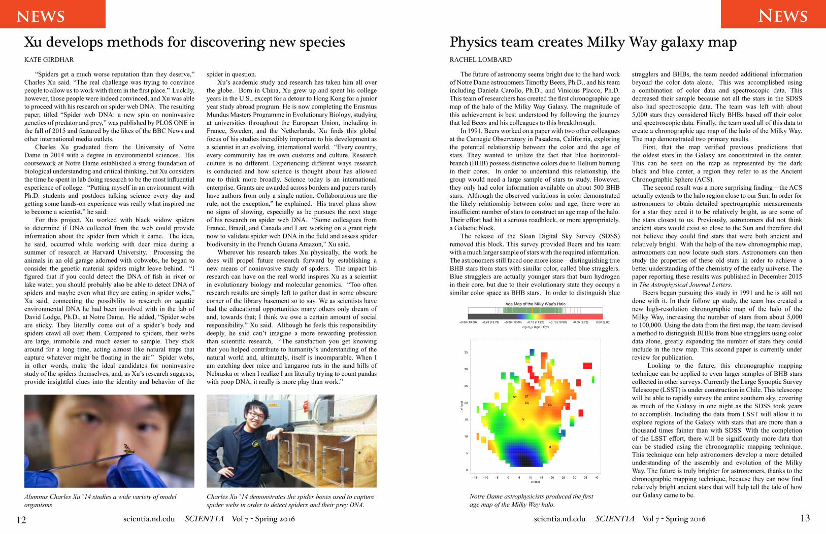
Charles Xu ’14 demonstrates the spider boxes used to capture spider webs in order to detect spiders and their prey DNA.

Alumnus Charles Xu ’14 studies a wide variety of model organisms

Xu develops methods for discovering new speciesKATE GIRDHAR

“Spiders get a much worse reputation than they deserve,” Charles Xu said. “The real challenge was trying to convince people to allow us to work with them in the first place.” Luckily, however, those people were indeed convinced, and Xu was able to proceed with his research on spider web DNA. The resulting paper, titled “Spider web DNA: a new spin on noninvasive genetics of predator and prey,” was published by PLOS ONE in the fall of 2015 and featured by the likes of the BBC News and other international media outlets.

Charles Xu graduated from the University of Notre Dame in 2014 with a degree in environmental sciences. His coursework at Notre Dame established a strong foundation of biological understanding and critical thinking, but Xu considers the time he spent in lab doing research to be the most influential experience of college. “Putting myself in an environment with Ph.D. students and postdocs talking science every day and getting some hands-on experience was really what inspired me to become a scientist,” he said.

For this project, Xu worked with black widow spiders to determine if DNA collected from the web could provide information about the spider from which it came. The idea, he said, occurred while working with deer mice during a summer of research at Harvard University. Processing the animals in an old garage adorned with cobwebs, he began to consider the genetic material spiders might leave behind. “I figured that if you could detect the DNA of fish in river or lake water, you should probably also be able to detect DNA of spiders and maybe even what they are eating in spider webs,” Xu said, connecting the possibility to research on aquatic environmental DNA he had been involved with in the lab of David Lodge, Ph.D., at Notre Dame. He added, “Spider webs are sticky. They literally come out of a spider’s body and spiders crawl all over them. Compared to spiders, their webs are large, immobile and much easier to sample. They stick around for a long time, acting almost like natural traps that capture whatever might be floating in the air.” Spider webs, in other words, make the ideal candidates for noninvasive study of the spiders themselves, and, as Xu’s research suggests, provide insightful clues into the identity and behavior of the

spider in question. Xu’s academic study and research has taken him all over

the globe. Born in China, Xu grew up and spent his college years in the U.S., except for a detour to Hong Kong for a junior year study abroad program. He is now completing the Erasmus Mundus Masters Programme in Evolutionary Biology, studying at universities throughout the European Union, including in France, Sweden, and the Netherlands. Xu finds this global focus of his studies incredibly important to his development as a scientist in an evolving, international world. “Every country, every community has its own customs and culture. Research culture is no different. Experiencing different ways research is conducted and how science is thought about has allowed me to think more broadly. Science today is an international enterprise. Grants are awarded across borders and papers rarely have authors from only a single nation. Collaborations are the rule, not the exception,” he explained. His travel plans show no signs of slowing, especially as he pursues the next stage of his research on spider web DNA. “Some colleagues from France, Brazil, and Canada and I are working on a grant right now to validate spider web DNA in the field and assess spider biodiversity in the French Guiana Amazon,” Xu said.

Wherever his research takes Xu physically, the work he does will propel future research forward by establishing a new means of noninvasive study of spiders. The impact his research can have on the real world inspires Xu as a scientist in evolutionary biology and molecular genomics. “Too often research results are simply left to gather dust in some obscure corner of the library basement so to say. We as scientists have had the educational opportunities many others only dream of and, towards that; I think we owe a certain amount of social responsibility,” Xu said. Although he feels this responsibility deeply, he said can’t imagine a more rewarding profession than scientific research, “The satisfaction you get knowing that you helped contribute to humanity’s understanding of the natural world and, ultimately, itself is incomparable. When I am catching deer mice and kangaroo rats in the sand hills of Nebraska or when I realize I am literally trying to count pandas with poop DNA, it really is more play than work.”

Physics team creates Milky Way galaxy mapRACHEL LOMBARD

The future of astronomy seems bright due to the hard work of Notre Dame astronomers Timothy Beers, Ph.D., and his team including Daniela Carollo, Ph.D., and Vinicius Placco, Ph.D. This team of researchers has created the first chronographic age map of the halo of the Milky Way Galaxy. The magnitude of this achievement is best understood by following the journey that led Beers and his colleagues to this breakthrough.

In 1991, Beers worked on a paper with two other colleagues at the Carnegie Observatory in Pasadena, California, exploring the potential relationship between the color and the age of stars. They wanted to utilize the fact that blue horizontal-branch (BHB) possess distinctive colors due to Helium burning in their cores. In order to understand this relationship, the group would need a large sample of stars to study. However, they only had color information available on about 500 BHB stars. Although the observed variations in color demonstrated the likely relationship between color and age, there were an insufficient number of stars to construct an age map of the halo. Their effort had hit a serious roadblock, or more appropriately, a Galactic block.

The release of the Sloan Digital Sky Survey (SDSS) removed this block. This survey provided Beers and his team with a much larger sample of stars with the required information. The astronomers still faced one more issue—distinguishing true BHB stars from stars with similar color, called blue stragglers. Blue stragglers are actually younger stars that burn hydrogen in their core, but due to their evolutionary state they occupy a similar color space as BHB stars. In order to distinguish blue

stragglers and BHBs, the team needed additional information beyond the color data alone. This was accomplished using a combination of color data and spectroscopic data. This decreased their sample because not all the stars in the SDSS also had spectroscopic data. The team was left with about 5,000 stars they considered likely BHBs based off their color and spectroscopic data. Finally, the team used all of this data to create a chronographic age map of the halo of the Milky Way. The map demonstrated two primary results.

First, that the map verified previous predictions that the oldest stars in the Galaxy are concentrated in the center. This can be seen on the map as represented by the dark black and blue center, a region they refer to as the Ancient Chronographic Sphere (ACS).

The second result was a more surprising finding—the ACS actually extends to the halo region close to our Sun. In order for astronomers to obtain detailed spectrographic measurements for a star they need it to be relatively bright, as are some of the stars closest to us. Previously, astronomers did not think ancient stars would exist so close to the Sun and therefore did not believe they could find stars that were both ancient and relatively bright. With the help of the new chronographic map, astronomers can now locate such stars. Astronomers can then study the properties of these old stars in order to achieve a better understanding of the chemistry of the early universe. The paper reporting these results was published in December 2015 in The Astrophysical Journal Letters.

Beers began pursuing this study in 1991 and he is still not done with it. In their follow up study, the team has created a new high-resolution chronographic map of the halo of the Milky Way, increasing the number of stars from about 5,000 to 100,000. Using the data from the first map, the team devised a method to distinguish BHBs from blue stragglers using color data alone, greatly expanding the number of stars they could include in the new map. This second paper is currently under review for publication.

Looking to the future, this chronographic mapping technique can be applied to even larger samples of BHB stars collected in other surveys. Currently the Large Synoptic Survey Telescope (LSST) is under construction in Chile. This telescope will be able to rapidly survey the entire southern sky, covering as much of the Galaxy in one night as the SDSS took years to accomplish. Including the data from LSST will allow it to explore regions of the Galaxy with stars that are more than a thousand times fainter than with SDSS. With the completion of the LSST effort, there will be significantly more data that can be studied using the chronographic mapping technique. This technique can help astronomers develop a more detailed understanding of the assembly and evolution of the Milky Way. The future is truly brighter for astronomers, thanks to the chronographic mapping technique, because they can now find relatively bright ancient stars that will help tell the tale of how our Galaxy came to be. Notre Dame astrophysicists produced the first

age map of the Milky Way halo.

14 15scientia.nd.edu SCIENTIA Vol 7 - Spring 2016 scientia.nd.edu SCIENTIA Vol 7 - Spring 2016

Physics PhysicsThe means and RMS are nearly identical for each parameter, which tells us that the algorithm works equally well for pileup. Additionally, we compared the efficiencies, with the restrictions 10.0<|pr|<100.0 and |η|<1.0:

Figure 4. Efficiencies for Pileup and No Pileup.

Since more tracks are found with pileup samples, we expected that the pileup efficiencies might actually be greater. In theory, if all possible tracks are found, the algorithm will yield one hundred percent efficiency, but this includes fake rates in which every false track is constructed. Here the pileup efficiencies are slightly worse, but this is not statistically significant.

Restricting η In order to learn more about the geometry of the tracker, I

input code restricting the values of η for the simulated events and left every seeding layer turned on. This allowed for us to understand which sections of the tracker (barrel, end-cap, or overlap) had the best resolutions, efficiencies, and abilities at matching stubs to the final track. Figure 5 shows the resolution plots for pr and ϕ compared by η range. 0 < |η| < 1 was used for the barrel, 1 < |η| < 1.8 was for overlap, and 1.8 < |η| was for the end-cap only. The important information to take from this study is definitely the fact that the barrel performs the best: its bell curve is not as wide as the other η ranges.

Seeding StudyThe next step was to turn off all but one section of the tracker and plot the efficiency versus η for each layer of the barrel and

calorimeters, a superconducting solenoid, and a tracker placed in a series of muon chambers to detect muons (3); our results use μ- samples. In order to accommodate for the HL-LHC upgrade, CMS will upgrade its trigger systems. We are focused on the Level 1 Trigger, which is employed in dedicated hardware and currently receives information from the calorimeter and muon triggers. The purpose of a trigger is to determine which collisions are the most interesting to analyze (out of around one billion proton collisions per second) and to store only those events (around 100 per second), thus significantly reducing the data processed. Due to higher luminosity and more overlapping collisions, L1 Trigger rates will increase from 100 kHz to 750 kHz. The overarching project is to instrument the tracking detector with the L1 Trigger, which will be crucial in handling the larger amounts of data. We are in the design and prototyping stage, estimated to end around 2018.

Field-Programmable Gate Array Emulation CodeThe tracklet project is part of a collaboration between

five universities, including Notre Dame. The code that the project shares emulates a field-programmable gate array (FPGA) that will be implemented in the CMS upgrades. FPGA circuits used in the trigger will analyze one event’s worth of data in approximately one microsecond. Using a track trigger algorithm, the emulator constructs tracks based on event data from an input text file. The first step in the algorithm is to find pairs of hits in each layer of the detector, known as stubs. The trigger only cares about stubs indicating high-momentum tracks. The second step is to find a tracklet, or a pair of stubs, in two adjacent layers, called seeding layers. Given this tracklet, the final step is to extrapolate the particle’s entire path. The L1 Trigger uses a linearized chi-squared fit to compare the path with nearby, consistent stubs. It determines four parameters: transverse momentum pT, initial azimuthal angle ϕ, pseudorapidity η, and initial coordinate along the beam axis z0. Pseudorapidity is related to polar angle θ by:

η ≡ -ln[tan(θ/2)]

In order to measure the algorithm’s performance, we created resolution plots, which essentially compare the constructed track parameters with their actual values. We ran the code four times, varying the seeding layer used for track reconstruction. Below are the normalized distributions:

Figure 1. Resolutions by seeding layer.

Working with field-programmable gate array emulation code for the compact muon solenoid upgradeJOHN CHARTERS1, KAITLIN SALYER1

Advisors: Kevin Lannon1, Michael Hildreth1

1University of Notre Dame, Department of Physics

AbstractWithin the next decade, the Large Hadron Collider (LHC)

will be upgraded to the High Luminosity LHC (HL-LHC). The upgrades will increase the number of particles in the accelerator in order to produce more collisions. The Compact Muon Solenoid (CMS) will require an enhanced trigger system to manage all of these interactions and determine which events to save. Primarily, we are trying to apply the tracking detector algorithms with the Level 1 Trigger. Our project relied on event simulations using an FPGA Emulation code developed by a team of physicists. The first half of this research involved evaluating the effectiveness of the algorithm to correctly identify particle tracks, provided samples with or without pileup. The other studies search for answers to a series of questions about the geometry of the detector and which seeding options were best at reconstructing the full tracks of particles after collisions. Much of this resulted from studying resolution of four track parameters and efficiency after restricting the pseudorapitidy, η.

The Large Hadron Collider and High Luminosity LHCThe Large Hadron Collider (LHC) is a particle accelerator

located at the European Organization for Nuclear Research (CERN). With a 27 kilometer circumference, the LHC is the largest and most powerful accelerator in the world. The collider consists of two particle beams traveling in opposite directions at nearly the speed of light, guided by superconducting electromagnets (1). As of April 2015, the beams collide at unprecedented energies of 13 TeV. The High Luminosity LHC is an ongoing project aimed at increasing the luminosity, a measure of the number of particles per unit area per unit time, to 10 times its current design value of 1034 cm-2 sec-1. The upgrades will improve the accuracy of the accelerator and allow for the detection of rare collisions (2). The HL-LHC is estimated to be installed around 2025, and will likely lead to physics discoveries beyond the Standard Model, such as more information on dark matter and supersymmetry.

Compact Muon Solenoid UpgradesThe Compact Muon Solenoid (CMS) is a detector at the

LHC that observes a range of particles in order to help answer the most fundamental questions in physics. Among other components, it consists of both electromagnetic and hadron

The performances of the first and second layers and all layers seeded almost completely match. Notice that the resolution for the outer layers is worse for η and z0. Initial attempts to improve these resolutions have been unsuccessful. Interestingly, the root mean square (RMS) for the fifth and sixth seeding layers is slightly smaller than that of all layers for pr and ϕ, signifying better results. It is also still unclear as to whether the resolution should depend on seeding layer at all. These questions are still being investigated. Next we plotted corresponding efficiencies for all parameters. We set the restrictions |pr |>10.0 and |η|<1.0:

Figure 2. Efficiencies by Seeding Layer.

The fifth and sixth layers have worse efficiencies than the other layers do. In general, we observed that the efficiencies are independent of parameter value, besides the fifth and sixth layer dip as η approaches 0. Overall the resolutions and efficiencies display great performance for the emulation code.

Comparison with Pileup SamplesOur previous studies used text files that represented single

muon samples without pileup. Pileup is a term used to indicate that multiple interactions are taking place per event in the same beam collision. Given the expected increase in collisions at higher luminosities, a more realistic sample includes pileup, where for each event the tracker finds thousands of stubs with hundreds of corresponding tracks. The tracking algorithm has more difficulty matching stubs with tracks, and consequently pileup events are harder to analyze. In order to evaluate the tracker’s precision with pileup samples, we compared the resolutions with no pileup samples. We turned all seeding layers on for these plots:

Figure 3. Resolutions for Pileup and No Pileup.Figure 5. Plots comparing the resolution of pr and ϕ for different ranges of η.

17scientia.nd.edu SCIENTIA Vol 7 - Spring 2016

HEALTH

16 scientia.nd.edu SCIENTIA Vol 7 - Spring 2016

Physicsthe end-cap. Figure 6 shows the plot resulting from that. L12 of the barrel gives the broadest coverage of the tracker, maintaining high efficiency in regions which would otherwise be missed by other combinations of the tracker. From this plot, the ranges of highest efficiency for each region were selected for further investigation.

Figure 6. Tracking efficiency plotted against η for each seeding option.

Running the emulation code with only one seeding option turned on and a restriction in η corresponding to the range of its highest efficiency, provided the ability to compare resolutions for each parameter in the most basic form. Figure 7 shows these resolution plots, but one further step could be taken: plotting only the tracks with six stubs matched to the final track. Figure 8 shows these results. The major difference between the plots with all tracks and those with only the full track reconstruction is that all the layers of the barrel perform about the same when all six stubs are matched.

Figure 7. The resolution plots for each seeding option with its respective restrictions in η. (FB34 not shown because the code provided empty files).

Figure 8. Resolution plots for pr ϕ for each seeding option with its respective η range and full track reconstruction.

Conclusion and Further WorkThe main studies on the algorithm’s performance have

shown that the FPGA Emulation code can successfully construct the path of a particle over the course of thousands of events. While there is some dependence on the layers used to seed, the results are overall favorable. Outer layer seeds tend to be less efficient and precise as one varies η and z0. We attempted to resolve the issue by making small changes to the code; this task proved futile, but it helped the code writers better understand alternative methods we could try in the future. We might also return to more in-depth pileup studies for further comparisons. From our other investigations, we can determine that the best seeding comes from the barrel, especially L12. By comparing the seeds based on their respective η ranges of highest efficiency, much of the extraneous information that clouded our initial studies was removed and this conclusion became clear. The next studies might include looking at nmatch as a function of η. This would help us understand simultaneously the geometry of the tracker and its abilities to match stubs to final tracks.

Acknowledgments We would like to give thanks to our advisors, Professor

Lannon and Professor Hildreth, for providing us with this research experience and the knowledge we have received from them. We would also like to thanks the CMS group whom we have been working with for providing us with questions and ideas to keep doing our research. Finally, we would like to thank Professor Garg for letting us be part of the Notre Dame 2015 Physics REU and for taking care of all the students from the REU.

References1.“The Large Hadron Collider.” CERN, n.d. Web. 28 July 2015.2. “The High Luminosity Large Hadron Collider.” CERN, n.d. Web. 28 July 2015.3.“Detector Overview.” CMS, 23 Nov. 2011. Web. 28 July 2015.

Effectiveness of an intensive exercise program for Parkinson’s DiseaseATTICUS COSCIA1

Advisors: Jennifer Robichaud1, Elizabeth Zauber2

1University of Notre Dame, Department of Biological Sciences2Indiana University School of Medicine, Department of Neurology

Abstract Parkinson’s disease (PD) is a common neurological

disease with no known cure. Rock Steady Boxing, a community-based exercise program for individuals with PD was studied to analyze the effects that this program has on its participants. Baseline evaluations of general strength, flexibility, coordination, balance, motor skills and quality of life were conducted when participants entered the program. Participants were then re-evaluated using the same measures at six month intervals for up to 24 months to determine the effect of the exercise program on PD symptoms and general fitness. For the 91 subjects that participated, at the one and two year follow-ups there were statistically significant improvements in upper and lower body strength, coordination, balance, and motor skills. General flexibility and quality of life were unchanged. Despite the expected worsening over time that traditionally accompanies a neurodegenerative disease such as PD, the Rock Steady participants who completed these assessments not only maintained physical function but showed improvements on the majority of the measures. While there are some limitations to the study design, these results suggest that exercise may be affecting neuroplastic changes in the PD brain, with possible neuroprotective effects.

IntroductionParkinson’s disease (PD) is a common neurodegenerative

disease with no known cure. PD is characterized by postural instability and rigidity, tremors, and decreased amplitude and speed of movement, termed bradykinesia. These symptoms are caused by a loss of dopaminergic neurons in the brain (1). While there are medical treatments for the disease, including pharmacological approaches and deep brain stimulation surgical procedures, none have been shown to slow the progression of the disease. Until recently, exercise was not recommended for PD patients as it was not known to have any effect upon the pathology of the disease. Recent studies, however, have shown that exercise holds a great deal of promise as a treatment for PD. Research focused upon traditional forms of exercise such as aerobic exercise and strength training have found that these activities can be successful therapeutic approaches to combating many of the clinical manifestations of PD (2-6). Aerobic exercise has been shown to have immediate beneficial effects in the improvement of gait, balance, and motor function,

with some studies noting significant changes in as little as 3 to 4 weeks of aerobic training (2, 7-8). Strength training has been shown to significantly improve mobility (3). The PD symptom of impaired gait has been improved using physical therapy (6). Exercise has also been correlated with improvement in non-motor symptoms associated with PD such as anxiety, depression, and fatigue (9-10).

Other studies have suggested that exercise may be able to alter the progression of PD. Preliminary data from animal studies suggests that exercise may slow the rate of neurodegeneration (1). The most effective forms of exercise for those with PD have also been investigated. Exercise has been shown to be especially effective when administered in a forced environment, such as a fitness class, or group setting, as opposed to being undertaken on a voluntary basis (1,11). These findings on forced exercise for PD patients suggest that the afferent feedback received by the brain from this activity may lead not only to improvements in motor functioning but also increased motor cortical activation and improved motor function in non-exercised effectors (11). Other novel approaches include the use of less traditional exercise forms as treatment options, such as Tai Chi or Tango classes. These classes, often administered in group settings, have shown promise in the improvement of movement and balance (12-13).

Despite the potential benefits of exercise for those with PD, the activity levels within the affected population are disturbing. A study conducted on a large sample group (n=699) in 2011 suggested that those affected with PD were on average one third less active than healthy controls (14). Other studies have likewise found increases in sedentary behavior and poorer physical conditioning in the Parkinsonian population (15-16). The neurodegenerative pathology of PD is disabling in its own right, but when coupled with physical inactivity it can be especially debilitating. In light of these findings, research geared toward the development of Parkinson’s-specific exercise options is especially pertinent. A novel approach to exercise for those with PD has been the application of boxing training techniques. This option was first explored by the founders of Rock Steady Boxing in 2006.

Rock Steady Boxing (RSB) is a non-contact, boxing-inspired fitness training class designed for individuals with PD that provides a forced exercise-type program. RSB was started in Indianapolis by former Marion County prosecutor Scott Newman and aims to improve the quality of life of PD patients. Classes are offered at four different levels roughly corresponding to the Hoehn Yahr scale of PD severity (mild motor dysfunction or impairment = scores of 0-2; moderate or severe impairment = scores of 3-4) (17). RSB classes combine, strength, agility, flexibility, and balance training. The RSB exercise program requires participants to dynamically alter and adjust their balance, posture, and base of support (18). The boxing training used also involves the coordination of throwing punches with foot movement. In addition, general stretching and strengthening exercises for both the upper and lower body are incorporated into the classes. One prior study of the program evaluated seven patients who were new to RSB. Subjects received a baseline evaluation of balance, gait, activities of daily life, and quality of life and were revaluated

About the AuthorKaitlin Salyer is a sophomore with a double major in physics and French, and a concentration in applied physics. She has worked on this project for the past year. She is excited that she will be studying abroad in Geneva, Switzerland, and working at CERN in Spring 2017. She hopes to look into other projects regarding the CMS upgrade as well as other CERN experiments during her study abroad experience.

About the AuthorJohn Charters is a sophomore with a double major in physics and honors mathematics from Woodinville, Washington. He began research his freshman year and participated in the Notre Dame Physics REU program in the summer of 2015.

18 19scientia.nd.edu SCIENTIA Vol 7 - Spring 2016 scientia.nd.edu SCIENTIA Vol 7 - Spring 2016

HEALTH HEALTHevery 12 weeks for 36 weeks. The study found that despite the progressive nature of PD, subjects showed short-term and long-term improvements in balance, gait, activities of daily living, and quality of life (18). While these results are promising, further research is needed on the long-term effects of RSB on PD symptoms and disease progression.

RSB has been collecting data on most of the participants since early 2011 with baseline and bi-yearly evaluations of fitness, balance, quality of life, and fine motor function. The reassessment measures are shared with the boxers to track personal progress and used by the trainers and staff for the purpose of class structure and planning. However, this data, to date, has not been analyzed. We performed a preliminary analysis to serve as pilot data for future externally funded research. We anticipate the results will also be useful to the organization in their future program development. We hypothesized that RSB participants would improve on the measures related to balance, mobility, flexibility, coordination and strength, dexterity, and quality of life.

Materials and MethodsThe RSB participants evaluated were residents of the greater

Indianapolis area and joined the program on a voluntary basis. The data analyzed in this study was collected and stored at the RSB headquarters facility in Indianapolis, Indiana. All RSB participants receive a baseline evaluation when they express interest in joining the program. This evaluation is used to place the individual in the proper class level for his or her PD severity and physical fitness. Disease severity is determined using the Hoehn Yahr scale, which roughly corresponds to the difficulty of the class levels. Participants were reevaluated every six months for up to two years. The baseline assessments, and following reassessments, consisted of the Fullerton Advanced Balance Scale (FAB), Timed Up and Go (TUG), Sit & Reach, Davies Test, Jump Rope test and the Purdue Pegboard test. Subjects were also encouraged to fill out a quality of life self-assessment, the 39-item Parkinson’s Disease Questionnaire (PDQ-39).

The FAB, comprised of 10 balance-related test measures, is a recently developed test designed to measure balance in higher-functioning older adults (19). The individual being measured receives a score of 0-4 on each measure, with the highest possible score of 40 corresponding to the best balance. For the TUG, subjects are timed as they rise from a seated position in a standard arm chair, walk a distance of ten feet, or three meters, away from the chair and finally return to the chair and sit down. The TUG test has been found to be an accurate assessment tool for individuals with PD, especially for predicting fall risk (20).

The Sit & Reach test is a common measure of hamstring and lower back flexibility. In this test subjects reach toward their toes and the distance that they deviate from a set point is measured. The Davies test is a measure of upper body and core strength and stability. This test involves maintaining a push-up position with the participant’s hands 36” apart. The subject then touches one hand with the other, alternating between hands, for as many repetitions as possible in fifteen seconds. In the Jump Rope measure, participants attempted to maximize the number of times they could jump over a rope that they swung in one minute. The Jump Rope task was intended to measure lower

body strength and stability, and coordination between the upper and lower body. These measures were used to assess the general fitness of the Rock Steady participants. Upper and lower body strength and stability, coordination between the upper and lower body, and general flexibility were tested with these measures.

The Purdue Pegboard test is a measure commonly used in studies to determine manual dexterity and bimanual coordiantion (21-22). To complete the Purdue Pegboard test, the participant attempts to place as many pegs as possible into a row of 25 matching holes on a board in 30 seconds. An average score from three tests for each hand was used. The manual dexterity and bimanual coordination required to complete the Purdue Pegboard test with some success are functionally fine motor skills.

The PDQ-39 is a 39 item Parkinson’s Disease Questionnaire intended to measure health-related quality of life. It has been suggested that this measure is a good indicator of mood functioning in PD patients (23). When filling out the questionnaire, participants rated 39 questions on a scale of 1 to 5. One represented an ideal score and 5 the most severe impairment possible; thus the best possible score on this measure was a 39 and the worst possible score a 195.

The results from the baseline tests and reevaluations were entered into a database and analyzed using a simple repeated measures analysis to determine if there was change between the respective evaluations. The repeated measures analysis was conducted using SAS Proc Mixed.

ResultsBetween early 2011 and late 2015, 91 individuals had

received a baseline evaluation and at least one reassessment (Table 1). Eight individuals received a baseline evaluation and were reevaluated up to four times, in a two year evaluation process. The average age of study participants was 70.03 years, while the age range of participants was 44-89 years. The average disease duration for study participants was 7.28 years. The disease duration range was 2-31 years. The statistical analysis of the data revealed significant increases in scores for the FAB assessment (p<0.0001, Figure 1), TUG test (p<0.0001, Figure 2), Davies test (p<0.0001, Figure 3), Jump Rope measure (p<0.0001, Figure 4), the right-hand portion of the Purdue Pegboard test (p<0.0004, Figure 5) and the left-hand portion of the Purdue Pegboard test (p=0.0036, Figure 6). The FAB results presented a mean score increase from 32.06±8.08 at the baseline evaluation to 38.13±1.64 at the fourth and final reevaluation. The TUG mean times decreased from 10.45±4.82 to 5.36±1.19 seconds, while the mean number of repetitions in the Davies test increased from 5.9±5.97 to 15.43±4.79 during this period. The Jump Rope test means likewise increased from 23.4±24.19 to 62.14±31.04 repetitions. Both of the Purdue Pegboard mean scores for number of pegs successfully placed increased as well, from 9.70±2.55 to 11.10±2.83 and from 9.60±2.48 to 11.18±2.48, for the right and left hands respectively. The Sit & Reach (p=0.0903, Figure 7) and the PDQ-39 (p=0.2245, Figure 8) did not present significant changes between evaluations. However, the PDQ-39 did show a general downward, and thus favorable trend, though this trend was not significant. Repeated measures analysis was also performed using the data collected

Table 1. Age and disease duration values for the study population.

Figure 1. Repeated measure analysis for the AB. There was a significant increase in scores for this measure across evaluations (p<0.0001).

Figure 2. Repeated measure analysis for the TUG test. There was a significant reduction in time across evaluations (p<0.0001).

Figure 3. Repeated measures analysis for the Davies test. Davies test scores increased significantly across evaluations (p<0.0001).

Figure 4. Repeated measures analysis for the Jump Rope measure. Scores for Jump Rope increased significantly across evaluations (p<0.0001).

Figure 5. Repeated measures analysis for the right hand portion of the Purdue Pegboard test. There was a significant difference across evaluations for this measure (p<0.0004).

Figure 6. Repeated measures analysis for the left hand portion of the Purdue Pegboard test. There was a significant difference across evaluations for this measure (p=0.0036).

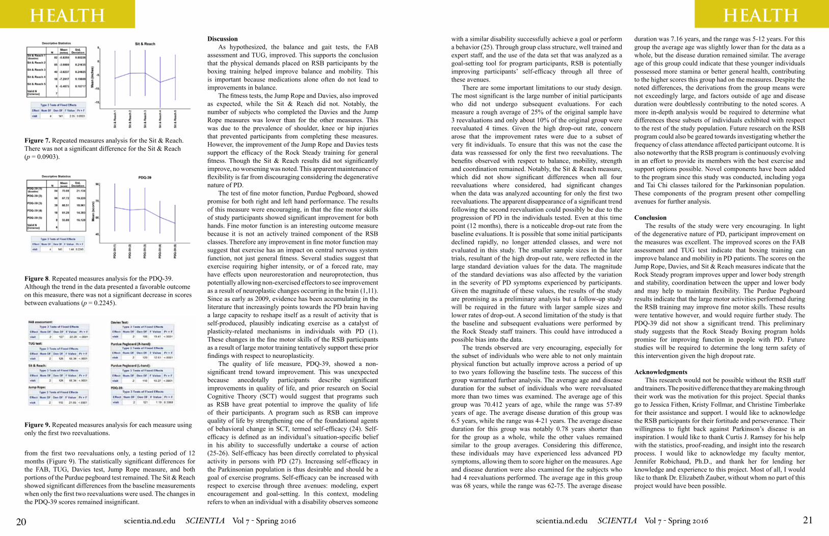
20 21scientia.nd.edu SCIENTIA Vol 7 - Spring 2016 scientia.nd.edu SCIENTIA Vol 7 - Spring 2016

HEALTH HEALTH

from the first two reevaluations only, a testing period of 12 months (Figure 9). The statistically significant differences for the FAB, TUG, Davies test, Jump Rope measure, and both portions of the Purdue pegboard test remained. The Sit & Reach showed significant differences from the baseline measurements when only the first two reevaluations were used. The changes in the PDQ-39 scores remained insignificant.

DiscussionAs hypothesized, the balance and gait tests, the FAB

assessment and TUG, improved. This supports the conclusion that the physical demands placed on RSB participants by the boxing training helped improve balance and mobility. This is important because medications alone often do not lead to improvements in balance.

The fitness tests, the Jump Rope and Davies, also improved as expected, while the Sit & Reach did not. Notably, the number of subjects who completed the Davies and the Jump Rope measures was lower than for the other measures. This was due to the prevalence of shoulder, knee or hip injuries that prevented participants from completing these measures. However, the improvement of the Jump Rope and Davies tests support the efficacy of the Rock Steady training for general fitness. Though the Sit & Reach results did not significantly improve, no worsening was noted. This apparent maintenance of flexibility is far from discouraging considering the degenerative nature of PD.

The test of fine motor function, Purdue Pegboard, showed promise for both right and left hand performance. The results of this measure were encouraging, in that the fine motor skills of study participants showed significant improvement for both hands. Fine motor function is an interesting outcome measure because it is not an actively trained component of the RSB classes. Therefore any improvement in fine motor function may suggest that exercise has an impact on central nervous system function, not just general fitness. Several studies suggest that exercise requiring higher intensity, or of a forced rate, may have effects upon neurorestoration and neuroprotection, thus potentially allowing non-exercised effectors to see improvement as a result of neuroplastic changes occurring in the brain (1,11). Since as early as 2009, evidence has been accumulating in the literature that increasingly points towards the PD brain having a large capacity to reshape itself as a result of activity that is self-produced, plausibly indicating exercise as a catalyst of plasticity-related mechanisms in individuals with PD (1). These changes in the fine motor skills of the RSB participants as a result of large motor training tentatively support these prior findings with respect to neuroplasticity.

The quality of life measure, PDQ-39, showed a non-significant trend toward improvement. This was unexpected because anecdotally participants describe significant improvements in quality of life, and prior research on Social Cognitive Theory (SCT) would suggest that programs such as RSB have great potential to improve the quality of life of their participants. A program such as RSB can improve quality of life by strengthening one of the foundational agents of behavioral change in SCT, termed self-efficacy (24). Self-efficacy is defined as an individual’s situation-specific belief in his ability to successfully undertake a course of action (25-26). Self-efficacy has been directly correlated to physical activity in persons with PD (27). Increasing self-efficacy in the Parkinsonian population is thus desirable and should be a goal of exercise programs. Self-efficacy can be increased with respect to exercise through three avenues: modeling, expert encouragement and goal-setting. In this context, modeling refers to when an individual with a disability observes someone

Figure 7. Repeated measures analysis for the Sit & Reach. There was not a significant difference for the Sit & Reach (p = 0.0903).

Figure 8. Repeated measures analysis for the PDQ-39. Although the trend in the data presented a favorable outcome on this measure, there was not a significant decrease in scores between evaluations (p = 0.2245).

Figure 9. Repeated measures analysis for each measure using only the first two reevaluations.

with a similar disability successfully achieve a goal or perform a behavior (25). Through group class structure, well trained and expert staff, and the use of the data set that was analyzed as a goal-setting tool for program participants, RSB is potentially improving participants’ self-efficacy through all three of these avenues.

There are some important limitations to our study design. The most significant is the large number of initial participants who did not undergo subsequent evaluations. For each measure a rough average of 25% of the original sample have 3 reevaluations and only about 10% of the original group were reevaluated 4 times. Given the high drop-out rate, concern arose that the improvement rates were due to a subset of very fit individuals. To ensure that this was not the case the data was reassessed for only the first two reevaluations. The benefits observed with respect to balance, mobility, strength and coordination remained. Notably, the Sit & Reach measure, which did not show significant differences when all four reevaluations where considered, had significant changes when the data was analyzed accounting for only the first two reevaluations. The apparent disappearance of a significant trend following the second reevaluation could possibly be due to the progression of PD in the individuals tested. Even at this time point (12 months), there is a noticeable drop-out rate from the baseline evaluations. It is possible that some initial participants declined rapidly, no longer attended classes, and were not evaluated in this study. The smaller sample sizes in the later trials, resultant of the high drop-out rate, were reflected in the large standard deviation values for the data. The magnitude of the standard deviations was also affected by the variation in the severity of PD symptoms experienced by participants. Given the magnitude of these values, the results of the study are promising as a preliminary analysis but a follow-up study will be required in the future with larger sample sizes and lower rates of drop-out. A second limitation of the study is that the baseline and subsequent evaluations were performed by the Rock Steady staff trainers. This could have introduced a possible bias into the data.

The trends observed are very encouraging, especially for the subset of individuals who were able to not only maintain physical function but actually improve across a period of up to two years following the baseline tests. The success of this group warranted further analysis. The average age and disease duration for the subset of individuals who were reevaluated more than two times was examined. The average age of this group was 70.412 years of age, while the range was 57-89 years of age. The average disease duration of this group was 6.5 years, while the range was 4-21 years. The average disease duration for this group was notably 0.78 years shorter than for the group as a whole, while the other values remained similar to the group averages. Considering this difference, these individuals may have experienced less advanced PD symptoms, allowing them to score higher on the measures. Age and disease duration were also examined for the subjects who had 4 reevaluations performed. The average age in this group was 68 years, while the range was 62-75. The average disease

duration was 7.16 years, and the range was 5-12 years. For this group the average age was slightly lower than for the data as a whole, but the disease duration remained similar. The average age of this group could indicate that these younger individuals possessed more stamina or better general health, contributing to the higher scores this group had on the measures. Despite the noted differences, the derivations from the group means were not exceedingly large, and factors outside of age and disease duration were doubtlessly contributing to the noted scores. A more in-depth analysis would be required to determine what differences these subsets of individuals exhibited with respect to the rest of the study population. Future research on the RSB program could also be geared towards investigating whether the frequency of class attendance affected participant outcome. It is also noteworthy that the RSB program is continuously evolving in an effort to provide its members with the best exercise and support options possible. Novel components have been added to the program since this study was conducted, including yoga and Tai Chi classes tailored for the Parkinsonian population. These components of the program present other compelling avenues for further analysis. Conclusion

The results of the study were very encouraging. In light of the degenerative nature of PD, participant improvement on the measures was excellent. The improved scores on the FAB assessment and TUG test indicate that boxing training can improve balance and mobility in PD patients. The scores on the Jump Rope, Davies, and Sit & Reach measures indicate that the Rock Steady program improves upper and lower body strength and stability, coordination between the upper and lower body and may help to maintain flexibility. The Purdue Pegboard results indicate that the large motor activities performed during the RSB training may improve fine motor skills. These results were tentative however, and would require further study. The PDQ-39 did not show a significant trend. This preliminary study suggests that the Rock Steady Boxing program holds promise for improving function in people with PD. Future studies will be required to determine the long term safety of this intervention given the high dropout rate.

AcknowledgmentsThis research would not be possible without the RSB staff

and trainers. The positive difference that they are making through their work was the motivation for this project. Special thanks go to Jessica Fithen, Kristy Follmar, and Christine Timberlake for their assistance and support. I would like to acknowledge the RSB participants for their fortitude and perseverance. Their willingness to fight back against Parkinson’s disease is an inspiration. I would like to thank Curtis J. Ramsey for his help with the statistics, proof-reading, and insight into the research process. I would like to acknowledge my faculty mentor, Jennifer Robichaud, Ph.D., and thank her for lending her knowledge and experience to this project. Most of all, I would like to thank Dr. Elizabeth Zauber, without whom no part of this project would have been possible.

23scientia.nd.edu SCIENTIA Vol 7 - Spring 2016

Biology

22 scientia.nd.edu SCIENTIA Vol 7 - Spring 2016

HEALTHReferences1. M. Hirsch and B. Farley. Eur. J. Phys. Rehab. Med. 45, 215-229 (2009).2. H.-F. Shu et al. PLoS One. doi: 10.1371/journal.pone.0100503. (2014). 3. T. Cruickshank et al. Medicine. 94, 1-15 (2015). 4. C. Canning et al. Neurology. 84, 304-312 (2014). 5. L. Dibble et al. JNPT. 39, 85-92 (2015). 6. M. Ganesan et al. Arch. Phys. Med. Rehab. 96, 1557-65 (2015).7. M. Thaut et al. Mov Discord. 11, 193-200 (1996).8. I. Miyai et al. Arch. Phys. Med. Rehab. 81, 849-852 (2000).9. K. Dashtipour. Epub. doi: 10.1155/2015/586378. (2015).10. N. Lee et al. J. Phys. Ther. Sci. 27, 145-147 (2015).11. A. Ridgel et al. Neurorehab. Neural Re. 23, 600-608 (2009).12. T.-Y. Zhang et al. Am. J. Phys. Med. Rehab. 15, 921-929 (2015). 13. S. Romenets et al. Complement. Ther. Med. 23, 175-184 (2015). 14. M. van Nimwegen et al. J. Neurol. 258, 2214-2221 (2011).15. F. Goulart. Acta Fisiatr. 36, 51-57 (2012).16. S. Chastin et al. Movement Disord. 25, 2114-2120 (2010).17. C. Goetz et al. Movement Disord. 19, 1020-1028 (2004). 18. S. Combs et al. Phys. Ther. 91, 1-12 (2011). 19. P. Klein et al. Physiotherapy Canada. 63, 115-125 (2011). 20. J. Nocera et al. Arch. Phys. Med. Rehab. 7, 1300-1305 (2013). 21. E. Smits et al. J. Biomed. Health Inform. (Epub ahead of print), (2015). 22. E. Proud et al. Arch. Phys. Med. Rehab. 5, 794-799 (2010). 23. J. Jones et al. Parkinsonism Relat. D. 11, 1236-1241 (2014). 24. A. Bandura. Self-Efficacy: The Exercise of Control. New York, NY: Worth Publishers; 1997.25. T. Ellis et al. JNPT. 37, 85-90 (2013). 26. A. Bandura. Health Educ. Behav. 31, 143-164 (2004).27. T. Ellis et al. Phys. Ther. 91, 1838-1848 (2011).

Understanding phenotypes of lung cancer using the Cancer Genome Atlas

EDEL SAH1 Advisors: Meeta Pradham2, Matthew Palakal2

1University of Notre Dame, Department of Biological Sciences2Indiana University-Purdue University, School of Informatics

AbstractAs multi-level data analysis is becoming increasingly

critical for translational research, many researchers are using this analysis to discover correlations between biological and clinical data. The Cancer Genome Atlas (TCGA), a coordinated effort organized by the National Cancer Institute (NCI), is one of the largest public sources with comprehensive patient data on over 30 different types of cancer from over 6000 patients. This study investigated the predictive power of clinical features for discriminating stages of lung adenocarcinoma, a common type of lung cancer that affects over 40% of lung cancer patients. R, an open source statistics programming language, was used to perform Principal Component Analysis (PCA) to visualize separation of data. Also, with features that showed separation in data, hierarchical clustering was performed. The results indicate that there are discriminating clinical features that are present in Stage I – Stage IV lung cancer. This analysis will help to associate related genes across various stages of lung adenocarcinoma for obtaining stage-wise, phenotypic-genotypic associations in lung cancer.

IntroductionLung cancer is the leading cause of cancer death worldwide

among both men and women, while cancer is the second leading cause of death following heart disease (1). In efforts to find treatments to cancer, researchers have focused on genomic analysis of cancer cells and have successfully improved patient treatment with targeted gene therapy. For example, targeting epidermal growth factor receptor (EGFR) mutations with gefitinib, an EGFR tyrosine kinase inhibitor, has resulted in tumor regression in lung cancer patients (2). In addition to EGFR, recent studies have suggested that targeting mutations in proto-oncogenes such as BRAF, AKT1, ERBB2, and PIK3CA might be useful for treatment of lung cancer patients (3).

Recent evidences have shown the importance of multi-level data analysis for translational research. Therefore, the objective of this study was to identify the correlations between biological and clinical data using TCGA, a coordinated effort organized by the NCI, which hosts comprehensive patient data on over 30 different types of cancer from over 6000 patients (4). This study investigates the predictive power of clinical features for discriminating stages of lung adenocarcinoma in particular.

Clinical data analysis of clinical features collected by TCGA, which includes over 470 lung adenocarcinoma patients, will help associate related genes across various stages to obtain stage-wise, phenotypic-genotypic associations in lung cancer.

Materials and MethodsData collection and selection

Comprehensive clinical data for lung adenocarcinoma was obtained from TCGA data portal (https://tcga- data.nci.nih.gov/tcga/). This data consisted of over 200 clinical features for 470 patients. R (http://www.r-project.org/), an open source program for statistical analysis, was used for analysis. In order to run differential statistical tests, the availability of clinical features were verified by calculating the percentage of patients with data for each feature following the division of patients into different cancer stage groups. After the calculation, features either with a significant amount of data or relation to cancer were selected.

PCAPrincipal Component Analysis (PCA) was used to find the

most relevant set of features from the large set of features that showed significant variations among cancer stages. Twenty-four features remaining after data selection and cleaning were used. For PCA, R command prcomp() was used. Data generated by PCA was visualized using scatter plots. Scatter plots were generated with R command ggbiplot2() to visualize the most relevant set of features found by PCA. Features were added or deleted from scatter plots, and scatter plots were compared to determine whether certain features contributed to data separation with respect to cancer stages.

ClusteringAfter features that were useful for separating data with

respect to stages were selected by PCA, hierarchical clustering diagrams were generated to determine if any significant data separation was achievable. For hierarchical clustering, R command hclust() was used. To discriminate each stage element from another, R command sparcl() was used.

ResultsThe original data presented in TCGA had more than 200

clinical analysis features for over 470 patients. After data selection and cleaning, 24 features that either had data available from over 80% of the patients or strong correlation to lung cancer remained (Table 1). These features were used to run the PCA, and the resulting data was graphed on scatter plots. The scatter plots were analyzed to identify clinical features discriminating different stages of lung adenocarcinoma (Figure 1). From the 24 features initially selected, demographic information, such as age, race, and ethnicity did not seem to be a significant factor for discriminating stages of patients. EGFR mutation did not seem to be a significant factor either. Interestingly, a behavioral feature such as tobacco smoking history was not significant for discriminating cancer stages either. The number of years since a patient stopped smoking, on the other hand, was a significant factor for discriminating cancer stages. Clinical information for tumor status, such as metastasis indicator, was also critical for discriminating cancer stages. Plotting PCA graphs with seven

About the AuthorAtticus Coscia is a junior from Zionsville, Indiana, pursuing a major in Science-Business. At Notre Dame, Atticus is a member of lab of Anthony Serianni, Ph.D., in the Notre Dame Department of Chemistry and Biochemistry. Atticus is also a member of Dr. Dawn Gondoli’s Teen Learning Laboratory in the Notre Dame Department of Psychology. Outside of research, Atticus works under Professor Sarah West as an organic chemistry laboratory teaching assistant. Atticus is also a member of the Notre Dame Men’s Boxing Club, and has participated in the annual Bengal Bouts boxing tournament as a sophomore and junior in an effort to raise money for the Holy Cross Mission in Bangladesh. Upon graduation, he hopes to matriculate into medical school.

24 25scientia.nd.edu SCIENTIA Vol 7 - Spring 2016 scientia.nd.edu SCIENTIA Vol 7 - Spring 2016

Biology Biologyclinical features (ajcc_tumor_pathologic_pt, ajcc_nodes_patho-logic_pn, ajcc_metastasis_pathologic_pm, tumor_necrosis_percent, tumor_nuclei_percent, tumor_weight, tobacco_smoking_years_stopped) showed effective separation of the original data.

From the seven features, three features were selected for hierarchical clustering. Hierarchical clustering with metastasis indicator, lymph node status, and the degree of radial exten-sion (ajcc_pathologic_tumor_stage, ajcc_tumor_pathologic_pt, ajcc_nodes_pathologic_pn) divided the data by cancer stage clearly, indicating that stages could be categorized based on these clinical features (Figure 2).

Table 1. Availability of selected clinical features for each stage. Most of the selected features had above 80% patient data availability. EGFR mutation status was lowest with less than 15% data availability.

Figure 1. Scatter plots graphing different selected clini-cal features. (a) Data is not effectively separated with some features. (b) Separation of data can be observed with certain features (ajcc_tumor_pathologic_pt, ajcc_nodes_pathologic_pn, ajcc_metastasis_pathologic_pm, tumor_necrosis_percent, tumor_nuclei_percent, tumor_weight, tobacco_smoking_year_stopped). The separation of data demonstrates that the seven features are significant in discriminating lung cancer stages.

DiscussionPlotting the data analyzed by PCA showed that certain

features, such as tumor size and tumor weight, were useful in separating data into several categories. Performing hierarchical clustering with the above features also demonstrated clear clustering results, showing that it is possible to use clinical features to sort the original data according to different cancer stages. Unexpectedly, this study did not find EGFR mutation status to be significant for discriminating the cancer stage. This lack of correlation may be due to the fact that only around 15% of lung patients had EGFR mutation data. Nonetheless, the study highlights the importance in testing for key oncogenic genes and data gathering in patients.

In this study, PCA was primarily used to generate graphs (Figure 1) to visualize the level of data separation when certain features being added and deleted. However, while reducing redundancy among variables, meaningful data were also generated with this method, including coefficients linked to features that were involved in calculating principal components. Developing methods to effectively use this data in order to identify important clinical features may prove to be beneficial.

Figure 2. Hierarchical clustering with metastasis indicator, lymph node status, and the degree of radial extension. Red: Stage 1 Lung Cancer; Green: Stage 2 Lung Cancer; Blue: Stage 3 Lung Cancer; Cyan: Stage 4 Lung Cancer. Separation and categorization of data can be seen. The graph shows that cancer stages can be categorized and separated by 3 clinical features.

In conclusion, this study indicates that there are discriminating clinical features dealing primarily with phenotypic associations in lung cancer that are present in Stage I – Stage IV in lung cancer. Coupling these phenotypic clinical features with studies involving genotypic associations across various stages of cancer may provide useful genotypic-phenotypic associations in lung cancer. A comprehensive genotype-phenotype map will ultimately help researchers in prevention and identification of harmful symptoms associated with lung cancer.

References1. Siegel, R., J. Ma, Z. Zou and A. Jemal. CA- Cancer J. Clin. 64, 9-29 (2014).

2. Paez, J. G., P. A. Janne et al. Science. 304, 1497-1500 (2004).

3. Cancer Genome Atlas Research, N. Nature. 489, 519-525 (2012).

4. Zhao, Q., X. Shi et al. Brief Bioinform. (2014).

About the AuthorEdel Sah is a senior from Memphis, Tennessee, studying biological sciences and applied and computational mathematics and statistics at the University of Notre Dame. Edel spent his last summer at Indiana University-Purdue University Indianapolis with Meeta Pradhan and Mathew Palakal conducting research on utilizing system biology approaches to identify biomarkers in the cancer disease networks.

a)

b)

26 27scientia.nd.edu SCIENTIA Vol 7 - Spring 2016 scientia.nd.edu SCIENTIA Vol 7 - Spring 2016

Math Maththe daily logarithmic returns, and x̄ is the mean return in the sample. An annualized variance can be found by multiplying the raw variance by the number of trading periods in a year. For daily returns, this would be 252 periods. The classic estimator has well understood sampling properties and is simple to use, yet it is very inefficient in its use of data, as it only incorporates close prices. Additionally, it tends to converge to the true volatility very slowly.

Over the past twenty-five years, a number of attempts have been made to improve upon this estimator. Researchers have sought to derive refined estimators to better capture the true movement of an asset’s returns by incorporating daily trading ranges, namely, the opening price, closing price, and intraday high and low prices of an asset. This research has shown that under certain circumstances, an estimator that considers these additional price movements can have a theoretical efficiency that is many times higher than that of the classic estimator (3).

In statistics, efficiency is a measure of the optimality of an estimator. The more efficient the estimator, the fewer the observations that are required to achieve a given performance level. As the standard definition of market volatility, the classic estimator serves as the baseline with which to compare all other estimators. The relative efficiency of the classic estimator, σ2

c , and an alternative estimator, σ2

a , is defined as

E(c,a) = ___ [1.2]

If an estimator has an efficiency greater than 1, it has a smaller variance than the classic estimator and converges more quickly to the true value. For a sample data set, the estimator with the highest efficiency is the optimal estimator. Finding the optimal estimator will allow a trader to use smaller data sample to calculate the volatility.

There are several common estimators that can be used to measure historical volatility, including the Parkinson estimator, the Garman-Klass estimator, the Rogers-Satchell estimator, and the Yang-Zhang estimator. Other alternative estimators do exist, but these four equations are popular methods that have been widely studied and shown to converge to the true volatility (4). To use each of these estimators, the normalized stock prices are first calculated. Normalization is a statistical tool that is used to standardize data from different periods. For the intraday stock data, the normalized close, open, high, and low prices are defined as, ct = ln(Ct) - ln(Ot), ot = ln(Ot) - ln(Ct−1), ut = ln(Ht) - ln(Ot), and dt = ln(Lt) - ln(Ot), respectively. Ct is the close price on day t, Ot is the open price on day t, Ht is the high price on day t, and Lt is the low price on day t. Using this notation estimator, the Classic estimator in [1.1] can be written as

σ2c = ____ ∑ [(oi + ci)

2 - _ ∑ (oi + ci)]2 [1.3]

The subsequent alternative estimators that are introduced all try to improve upon the performance of the classic estimator. The first alternate volatility estimator was created by Parkinson in 1980 (3). The Parkinson estimator is calculated by looking at the high and low values of the asset and is defined as

σ2p = ____ ∑ (ui - di)

2 [1.4]

Where σ2

o = ____ ∑ ci2

and σ2c is defined as in [1.2] and σ2

RS is defined as [1.5]. The constant k is defined as:

k = ________

Although the Yang-Zhang estimator has been shown to have the greatest theoretical efficiency, it is also highly dependent on the proportion of volatility caused by opening jumps. Specifically, if these jumps dominate the overall volatility, its efficiency can fall to that of the classic estimator.

A key factor in determining which estimator to use when measuring historical volatility is understanding the assumptions that underlay each estimator and the conditions when these assumptions may not hold. Overwhelmingly, research in estimator selection has not supported the conclusion that theoretically optimal estimators will actually have the optimal performance in every situation. Instead, studies conducted with both stimulated and empirical data reinforce the idea that the relative performance of estimators is highly dependent on the characteristics of the data sample. To better understand the influence of market conditions on these estimators, testing them using a variety of data samples can provide interesting, and sometimes surprising, conclusions. The results section of this study contains three different experiments: a study on the effect of significant jumps in the asset price using simulated data, a study on the effect of non-zero drift using historical market data, and a study on the effect of the sample size using historical market data.

To manipulate market conditions, the simulated data was created using Monte Carlo simulation, discretizing the stock price formula using geometric Brownian motion:

St = S0 exp[(μ - __ )t + σWt] [1.8]

where Wt is Brownian motion, or the square root of t multiplied by a random variable that follows a standard normal distribution. In the simulation, each incremental stock price is calculated using this equation, with an initial stock price of $100. The data series assumes zero drift, constant annualized volatility of 0.14, and a sample period of 20 trading days. Stock prices are updated every five minutes, or the stock price moves 78 steps during the trading day. Once calculated, the volatility estimates were then annualized. The empirical market data was downloaded from Yahoo Finance.

ResultsPart I: Analyzing the effect of opening price gaps using simulated data

Scenario I: In the first scenario, there are no steps between the close price of one day and the opening price of the next. Using [1.8], the random stock motion generated for the first scenario exhibits a significant downward trend, and the price falls from

Alternative estimators for stock volatilityMELISSA KRUMDICK1

Advisor: Huy Huynh1

1University of Notre Dame, Department of Applied and Computational Mathematics and Statistics

AbstractA primary use of volatility in financial markets is to

determine market risk. Volatility is able to measure the riskiness of a financial asset by considering the spread of the asset’s return, a random variable that represents the gain or loss on the asset during a specific period. As the true volatility for an asset price is inherently unobservable, in order to identify profitable opportunities in the market, traders must rely on an estimator to calculate historical volatility. Research has shown that the classic estimator of volatility is frequently outperformed by more efficient alternative estimators. In this study, the performance of the Parkinson, Garman-Klass, Rogers-Satchell, and Yang-Zhang estimators is evaluated by testing the effect of asset price jumps, nonzero drift, and the sample size. Both simulated asset prices and empirical data are considered.

IntroductionIn recent years, the overall size of the derivatives industry

has quadrupled (1). As these instruments become more widely circulated, it is increasingly important for both professional traders and retail investors to understand how these securities can be utilized to optimize the performance of their portfolios. Derivatives can be used to achieve a variety of goals, including increased leverage, higher returns, and lower downside risk. In financial trading, the flexibility and versatility of option contracts is especially advantageous. Volatility-based option trading strategies aim to recognize mispriced options by comparing an option's estimates for historical and implied volatility and exploiting instances when the market view appears to be misestimating the option's volatility by trading a delta neutral portfolio of an option and its underlying (2).

With this methodology in mind, the key to determining potentially profitable trading opportunities is to identify an option that has a significant difference in its implied and historical volatility. Once a trader is able to calculate the implied volatility using the option's current market value, he needs to find some measure of historical volatility to compare this estimate. This research will consider several popular historical estimators that allow traders to contrast the market view with the historical view.

Materials and MethodsThe classic definition of volatility is the square root of the

variance of the asset returns where the variance is defined as

s2 = ____ ∑ (xi - x̄)2 [1.1]

In this formula, n is the length of the sample period, xi are

Because the Parkinson estimator incorporates an additional price from each day, it is more efficient than the classic estimator. This allows for it to converge to the true value more quickly. However, using an estimator based on an observed range like the Parkinson estimator will cause the volatility to be systematically underestimated. Because prices are discretely sampled and the market is only open for a portion of a day, the unobservable true price may reach a high or low at a time when it is not measured. In addition, the Parkinson estimator cannot handle jumps in the asset price, particularly when there is a significant gap between a closing price and the next day’s opening price. Notably, while other estimators are more efficient based on simulated data, some studies using empirical data have shown that the Parkinson estimator performs the best.

Later in 1980, the Garman-Klass volatility estimator was created as an extension to the Parkinson estimator (3). The Garman-Klass estimator is defined as:

σ2GK = ____ ∑ (ui+di)

2 - ____ ∑ [ci(ui+di) - 2uidi] - ____ ∑ ci

2

[1.5]

This estimator incorporates even more commonly available price information, improving upon the efficiency of the Parkinson estimator. However, it has been shown to exhibit an even more significant bias and still cannot incorporate jumps. Problematically, the efficiency of the Parkinson and Garman-Klass estimators rely on an assumption that does not always exist in real markets; both of these estimators assume that the asset follows a geometric Brownian motion process with zero drift. Although this assumption is a good approximation for a daily series when the asset price does not trend strongly, when these estimators are considered over longer periods, the drift can become quite large compared to its volatility. As a result, both the Parkinson and Garman-Klass estimators can be less effective (4).

In 1991, Rogers and Satchell derived an estimator that is better able to account for instances of nonzero drift (3). Their estimator, known as the Rogers-Satchell estimator, is defined

σ2RS = ∑ [ui(ui -ci) + di(di -ci)] [1.6]

By relaxing this zero drift restriction, the Rogers-Satchell estimator outperforms the Parkinson and Garman-Klass estimators when an asset price is trending strongly. However, it cannot handle jumps, hence it underestimates the volatility. In 2002, Yang-Zhang created the most powerful volatility estimator of those introduced so far, capable of both that handling opening jumps and non-zero drift. Calculated as a weighted average of the open to close volatility, the overnight volatility (close to open volatility), and the Rogers-Satchell volatility, the Yang-Zhang estimator has the minimum estimation error, or variance of the historical estimators considered (3). Consequently, it theoretically has the highest efficiency. The Yang-Zhang estimator is defined as

σ2YZ = σ2

o + kσ2c + (1-k)σ2

RS [1.7]

1n - 1

n

i = 1

σ2a

σ2c

n1n - 1

i = 1

1n

n

i = 1

14nln2

n

i = 1

0.511n

n

i = 1

0.019n

0.383n

n

i = 1

n

i = 1

n

i = 1

1n - 1

n

i = 1

1 + _____n + 1n - 1

1

σ2

2

28 29scientia.nd.edu SCIENTIA Vol 7 - Spring 2016 scientia.nd.edu SCIENTIA Vol 7 - Spring 2016

Math Math

approximately $100 to $60 over the sample period. A plot of the asset path and volatility estimates over the 1,000 trading day period are shown in the following figures.

Visually, the true volatility appears to lie between 0.1 and 0.2. As the constant annualized volatility was 0.14, it seems that all of the estimators do produce reasonable results. The classic estimator has the highest mean absolute deviation, and it produces both the minimum and maximum estimates. Looking at the plot of the volatilities, it is also clear that all five of the estimators produced highly correlated results. The average values and efficiencies of the five estimators from these two simulations are included in the following table. For computing the efficiency, the variance of each estimator is compared to the variance of the classic estimator, as the baseline estimator, as defined in [1.9].

When there is no drift term, constant volatility, and no steps

outside of the trading day, the performance of the alternative estimators is relatively similar. All of the estimators had a higher efficiency than the classic estimator, and the alternate estimators had the same average to two decimal places. Although the classic estimator has the greatest variance, and as

such, the lowest efficiency, its average value is relatively similar to the other estimators, so it is still useful for analysis. All of the estimators show a marked tendency to underestimate the true process volatility, as they fail to capture the true realized volatility without including more frequent intraday asset movements. This bias is decreased as the sampling frequency increases. The Parkinson and Yang-Zhang estimators performed the best, with efficiencies approximately seven times that of the classic estimator. However, considering the correlation of the estimates and the similarity of the results, all of the estimators were able to reasonably track the volatility, and there is no reason to assume any estimator is significantly misestimating volatility under these simulated market conditions.

Scenario II: A more accurate representation of asset movement would incorporate movement outside of the trading day by including a number of additional steps after the close price to account for opening price gaps. Scenario II models a situation where significant price jumps occur outside of the trading days, or there is a lot of overnight movement in stock price. This was modeled in the discretized stock motion equation by adding 200 steps outside of trading days. Like Scenario I, there is a downward trend overall, but the trend is more erratic, with the stock fluctuating at a price around $120 for the first 500 trading days, and hovering at a lower price around $80 for the second half of the study. The plot of the simulated asset walk for this experiment and the volatility estimates from the same five estimators using the new asset price motion are shown in the plots below.

Clearly, in this scenario, there is a significant discrepancy between several of the estimators. This discrepancy is better captured in the following table.

Unlike Scenario I, the presence of significant opening gaps has introduced a significant bias into two of the estimators: the classic estimator and the Yang-Zhang estimator. The difference in a day’s open and close prices are much higher when there is movement outside of trading hours, and both of these estimators produced volatility estimates with an average value of approximately 0.23, which is significantly greater than the annualized volatility of 0.14 used in the model. Alternatively, the Parkinson, Garman-Klass, and Rogers-Satchell estimators all have averages must closer to the model’s annualized volatility, with values of approximately 0.11. These estimators produced averages very similar to those found in Scenario 1. As the classic estimator does such a poor job of capturing the volatility, the efficiency of these three estimators is many times that of the classic estimator. Additionally, since the classic estimator is included in the weighted average that constitutes the Yang-Zhang estimator, even though the Yang Zhang estimator is theoretically the most efficient estimator, it actually has the lowest efficiency in this simulation, as proportionally, the asset movement is dominated by the opening price gaps. The results from Scenario II reinforce the importance of understanding how an asset price is moving when selecting an estimator for historical volatility. Depending on the asset’s path, different estimators may be better suited to predict future volatility. To further examine the performance of the estimators, Section 8.4 will use empirical market data to assess the impact of significant drift in the asset path.

Part II: Analyzing the effect of long-term drift using empirical data

To analyze the influence of a significant nonzero drift, the high, low, open, and close daily prices of two different assets were considered: The SPDR S&P 500 ETF Trust (stock ticker: SPY), a fund which seeks to provide investment results that, before expenses, correspond generally to the price and yield performance of the SP 500 Index and AT&T, Inc. (stock ticker symbol: T). From January 2013 through December 2015, the SPY experienced a significant positive drift, as the price increased approximately $50; during the same period, T

30 31scientia.nd.edu SCIENTIA Vol 7 - Spring 2016 scientia.nd.edu SCIENTIA Vol 7 - Spring 2016

Math Mathremained relatively flat, with prices fluctuating between $30 and $40. Similar to the simulated scenarios in Part I, the historical estimates were calculated over 1 month periods, or a series of trading 20 days. Once calculated, the volatility estimates were then annualized. The figures below show the plot of the annualized estimates over the sample period.

The five estimators appear to produce highly correlated estimates, typically fluctuating between 0.05 and 0.2 for SPY and 0.1 and 0.3 for T. For comparison, the efficiency of each estimator was calculated. The results of these calculations are shown in the following table.

In most instances, alternative volatility estimators improved upon the efficiency of the classic estimator. All of the alternative estimators had a higher efficiency for the AT&T data set than the SPY prices. For the SPY data, the Yang-Zhang estimator actually performed worse than the classic estimator. Again, higher theoretical efficiency can translate to higher actual efficiency, but this is not always the case. It appears that significant drift inhibits the performance of the estimators, most notably for the Garman-Klass estimator, which assumes zero drift and no opening jumps. The difference in the efficiency of the Garman-Klass estimator between the two stocks is almost a full point. As the true volatility of a stock with a long-term positive or negative trend may be harder to capture, it might be useful to include wider confidence intervals for estimates when the asset price path exhibits this trend.

Part III: Analyzing the effect of sample sizeAnother decision a trader has to make is selecting the sample

size of the data used to create an estimate. Larger samples smooth out outlier values but also require larger data sets. To examine the impact of the sample size on the performance of the estimators, the SPY data set from Part II was used. In this experiment, the estimates were calculated using three different sample sizes: 5, 25, and 50 day samples. The bias, mean absolute deviation (MAD), and efficiency of the estimators was calculated for each of the sample.

The results of this study show that increasing the sample size helps decrease the bias and mean absolute deviation of all of the estimators, or with a larger sample, accuracy is increased. The classic estimator exhibited the most significant increase in accuracy, as its performance is highly dependent on the size of the sample. As a result, the efficiencies of the alternative estimators decreased as the size of the sample increased. The order of relative efficiency, however, is not much changed by increasing the sample size. This study reinforces what we would

expect: using a larger sample increases accuracy. However, it does not suggest that the optimal estimator for a data set will change as the sample size varies.

Discussion The exhibits included in the results section are not a

comprehensive survey of all of the factors that can influence volatility estimator selection; rather, there exists a wide range of other factors that can impact performance. However, this discussion on historical volatility should explain how traders can become more comfortable understanding the relationships between estimators and the insights that can be gained from relative estimator performance.

Ultimately, the results of this study demonstrate that although theoretically the Yang-Zhang estimator is the most efficient, evidence suggests that under certain market conditions, other estimators can outperform the Yang-Zhang estimator. Although it may at first seem rational to rely on the theoretically best performing estimator to forecast future volatility, there is no universal recommendation for estimating historical volatility. It is at the discretion of a trader to compare estimators and use his best judgment when making estimation decisions. Since stock and index prices do not move uniformly, there is no single estimator that consistently outperforms the others; rather, traders trend to agree that volatility should be measured using a variety of estimators, with special attention given to the strengths and weaknesses of each method.

Some of the important factors that a trader can consider when determining his final historical estimate are:

•Are there extreme jumps in price?•Does the asset price experience significant drift?•How many trading days are included in each sample?

All of these factors can help a trader decide if the available asset data is being used most efficiently. Often, it is not one estimator that should be considered but a combination of several. A trader can even consider constructing a weighted average of estimators. Careful selection of the estimators that will be most useful for measuring volatility requires understanding which underlying assumptions are best met by the asset price’s movement. This makes determining estimates for historical volatility a more involved process, and makes the calculation and comparison of different estimators a more essential aspect of volatility trading. Often, this is an area in which a trader’s intuition and experience prove invaluable.

While important, the use of proper methodologies and equations is not enough to make a trader great. Instead, in trading, there is a very significant psychological component. As Ed Seykota, a commodities trader whose achievements earned him recognition as one of the best traders of his time, said, “Psychology motivates the quality of analysis and puts it to use. Psychology is the driver and analysis is the road map”(5). Historical volatility estimation is one area of trading that is highly psychological; with practice, great traders will be able to discern optimal historical volatility estimates and use these estimates to identify profitable trading opportunities.

About the AuthorMelissa Krumdick is a senior at the University of Notre Dame currently pursuing a degree in applied and computational mathematics and statistics and a minor in actuarial science. She is in the Glynn Family Honors Program. Krumdick has been involved in research since the summer after her sophomore year, when she was the project manager of an undergraduate research team in the Research in Industrial Projects for Students program at the Institute for Pure and Applied Mathematics at UCLA. Her current research interests are in the field of quantitive finance. Over the past two years, Krumdick has been analyzing the mathematical statistical techniques that underlie volatility-based option trading strategies for her senior thesis. After graduation, she will be working as a derivatives trader at a proprietary trading firm in Chicago.

References1. Hull, John. Options, Futures, and Other Derivatives. Upper Saddle River, NJ: Pearson/Prentice Hall, 2006. Print.

2. Sinclair, Euan. Volatility Trading. Hoboken, NJ: Wiley, 2008. Print.

3. Kinley, Jonathon, and Michael W. Brandt. “Estimating Historical Volatility.” (n.d.): n. pag. 07 May 2009. Web.

4. Bennett, Colin, and Miguel A. Gil. “Measuring Historical Volatility.” Equity Derivatives (2012): n. pag. 03 Feb. 2012. Web.

5. Schwager, Jack D. Market Wizards: Interviews with Top Traders. New York, NY: New York Institute of Finance, 1989. Print.

32 33scientia.nd.edu SCIENTIA Vol 7 - Spring 2016 scientia.nd.edu SCIENTIA Vol 7 - Spring 2016

Math MathDefinition. Two disjoint subsets A, B of a topological space (X, T ) can be separated by open sets if and only if there exist disjoint open sets U and V containing A and B respectively; i.e. ∃U, V ∈ T such that A ⊂ U, B ⊂ V , and U ∩ V = ∅.

Definition. Two disjoint subsets A, B of a topological space X can be separated by a continuous function if and only if there exists a continuous function f : X → [0, 1] such that f(A) = {0} and f(B) = {1}.

Note that since any closed interval [a, b] of ℝ is homeomorphic to [0, 1], the condition of A and B being separable by continuous function is equivalent to the existence of a continuous function g : X → [a, b] such that g(A) = {a} and g(B) = {b} for any given a < b ∈ ℝ.

Many interesting properties come from which separation axioms hold for a topological space; that is, which kinds of subsets of the space can be separated by open sets (or, in some cases, by continuous functions). The axiom invoked in Urysohn’s Lemma is that of normality:

Definition. A topological space is called normal if and only if each pair of disjoint closed sets can be separated by open sets.(Note that, for example, ℝ is a normal topological space).

An equivalent definition will be particularly useful for the proof of Urysohn’s Lemma; it states that normality is equivalent to being able to “fit” a set and its closure “in between” a given closed set and open set containing it:

Lemma 2.1. A topological space X is normal if and only if given any closed set A and any open set U containing it, there exists open V such that A ⊂ V and V ⊂ U.

Proof. Suppose X is normal. Let A be closed, U ⊃ A open. Then A and X − U are disjoint closed subsets of X; by normality, there exist disjoint open V, W such that A ⊂ V and X − U ⊂ W. The set X − W is a closed set containing V, so V ⊂ X − W. Furthermore, X − W ⊂ U, so V ⊂ U.

Now suppose the latter condition holds for X. To show that X is normal, let A, B bedisjoint closed subsets of X. Then X − B is an open set containing A. By hypothesis, there exists open V such that A ⊂ V ⊂ V ⊂ X − B; then X − V is an open set containing B which is disjoint from V ⊃ A.

We can now state and prove the first major theorem in this paper.

Remark 2.2. The theorem was first proved by the mathematician Pavel Urysohn in the early twentieth century. The method of proof given here is that of Munkres [2], and the notation used is usually similar if not identical. We have tried to make steps that Munkres skipped over or left to the reader more explicit.

Theorem 2.3. (Urysohn’s Lemma) Let (X, T ) be a normal topological space. Let A, B be disjoint, closed subsets of X. Then A and B can be separated by a continuous function.

Urysohn’s lemma and the Tietze extension theoremCHRISTIAN GORSKI1

Advisor: Frank Connolly1

1University of Notre Dame, Department of Mathematics

AbstractThe primary purpose of this paper is to prove two theorems

from point-set topology: the Urysohn Lemma and the Tietze Extension Theorem. We include a quick review of basic point-set topology, assuming familiarity with basic set theory and some real analysis. The exposition is heavily influenced by James R. Munkres’ Topology [2].

IntroductionWe begin with a brief review of the basics of point-set

topology. For a more thorough reference, see [2]. Point-set topology provides the most general context in

which the concept of a continuous map makes sense. This is accomplished through the notion of open sets. A subset U of ℝn is called open (in the standard topology) if for every point x ∈ U, there exists ε > 0 such that for all y ∈ ℝn with ∥y − x∥ < ε, y ∈ U. That is, for each x ∈ U, there is an “open ball” of nonzero radius centered at x which is contained completely in U. With this definition, it is not hard to prove the following proposition:

Proposition 1.1. A map f : ℝm → ℝn is continuous (i.e. continuous at each point of ℝm) if and only if for each open set V of ℝn, f−1 (V ) := {x ∈ ℝm|f(x) ∈ V } is an open set of ℝm.

Notice that this definition only refers to the spaces ℝm, ℝn and their open sets. Thus, if we want to extend the notion of continuity to maps between spaces more exotic than Rn, all we need to do is to define what it means for subsets of the spaces to be open. The set of open sets of a space is called the space’s topology. We make the following definition:

Definition. A topology T on a set X is a collection of subsets of X such that the following conditions hold:

1. Both the empty set ∅ and the entire space X are elements of T.2. T is closed under arbitrary unions; i.e.Uα ∈ T ∀α ∈ I ⇒ ⋃α∈I Uα ∈ T.3. T is closed under finite intersections; i.e. U ∈ T and V ∈ T ⇒ U ∩ V ∈ T.

The pair (X, T ) is called a topological space.

Remark 1.2. We sometimes denote the topological space (X, T ) simply by X.

The study of point-set topology is concerned with those properties which only depend a space’s topology. We now introduce concepts and propositions needed for our proofs:

We call an open set U which contains a point x a neighborhood of x. This reflects the intuition that each

neighborhood of x contains “a little area around x.” (This definition of neighborhood differs slightly from some other common definitions, but this makes no real difference for our purposes.)

Another convenient concept is that of a basis:

Definition. A basis ß for a topology T on a set X is a collection of subsets of X such that U ∈ T ⇔ U is a union of elements of ß.

Note that the collection of open balls (sets of the form B∈ (x0) := {x ∈ ℝn: ∥x−x0∥ < ε} for some fixed x0 ∈ ℝn, ε > 0) forms a basis for the standard topology on ℝn. Moreover, the collection of open intervals {(a, b)|a < b ∈ ℝ} forms a basis for the standard topology of ℝ.

Complements of open sets are called closed sets. It follows directly from this definition (and DeMorgan’s Laws) that the property of being closed is preserved under arbitrary intersection and finite union, and that ∅ and X are always closed sets of X. Note that, in general, a subset of X may be closed, open, both, or neither.

A particularly important concept is that of the closure of a set; to produce the closure of a set, we “add just enough points to make it closed.” Formally, we define it thus:

Definition. The closure (denoted Ā) of a subset A of a topological space (X, T) is the intersection of all closed sets of X which contain A.

It is easily seen that Ā is itself a closed set containing A and that any closed set containing A contains Ā.

We define continuity of maps between topological spaces as suggested by Proposition 1.1:

Definition. Let X, Y be topological spaces, f : X → Y . Then f is continuous if and only if for every open set V of Y , f −1(V ) is open in X.

It is not hard to show from this definition that preimages of closed sets under continuous maps are closed. In addition, it is easily shown that compositions of continuous functions are continuous. Here is an equivalent notion of continuity which we will use in the proofs of the main theorems:

Proposition 1.3. Let X, Y be topological spaces, f : X → Y . Then f is continuous if and only if for each x ∈ X and each basis element B of Y containing f(x), there exists a neighborhood U of x in X such that f(U) ⊂ B.

There is not one “correct” topology that can be determined by examining a set. However, given existing topological spaces, there exist natural ways of defining other topological spaces which relate to them—in particular, once we have determined a topology T on a set X, there is a natural way to define a topology on a subset A ⊂ X.

Definition. Let (X, T ) be a topological space, and let A ⊂ X. A subset U ⊂ A is open in the subspace topology of A if and only if there exists U' ∈ T such that U = U' ∩ A.

This definition is natural in the sense that the inclusion map ι : A → X, ι(a) = a is continuous when A is given the subspace topology. It is also easily seen (from the intersection properties of closed sets) that if A is a closed set of X which is given the subspace topology, and B is a closed set of A, then B is a closed set of X. (A similar statement holds for open sets). Throughout this paper, all subsets will be assumed to have the subspace topology.

Furthermore, assuming the subspace topology, we have the following:

Proposition 1.4. Let f : X → Y be a continuous function. Then the following hold:

(i) f : X → f(X) is continuous.(ii) If Y is a subspace of some topological space Z then f : X → Z is continuous.(iii) If A is a subset of X, then f|A : A → Y is continuous.

Put simply, we may restrict or expand the codomain without affecting the continuity of a function (keeping in mind that if we restrict the codomain too much, we must also restrict the domain). In particular, proving that a function is continuous to ℝ amounts to showing that it is continuous to any subspace of ℝ containing the function’s range.

The last topological concept we introduce will simplify our main proofs quite a bit.

Definition. Let X and Y be topological spaces. A function h : X → Y is a homeomorphism if and only if h is bijective, h is continuous, and h−1 is continuous. Furthermore, if such a function exists, X and Y are said to be homeomorphic.

Homeomorphisms are of fundamental importance because they establish a sort of “topological equivalence” between two spaces. Any property of a given space which is a topological property—that is, a property which is expressed only in terms of the space’s topology—must also be held by any space homeomorphic to the given space. This is because if X and Y are homeomorphic, any open set in X has a corresponding open set in Y and vice versa.

The following homeomorphisms will be useful to us:

Proposition 1.5. Let a, b, c, d ∈ ℝ be such that a < b and c < d. Then [a, b] is homeomorphic to [c, d] by means of the homeomorphism h(x) = (____)(x − a) + c.

Proposition 1.6. (−1, 1) is homeomorphic to ℝ by means of the homeomorphism h(x) = tan(πx).

Urysohn’s LemmaWe now have almost enough background to state and prove Urysohn’s Lemma, the first major theorem presented this paper. Up to this point, most of the propositions stated have followed simply from definitions. The proof of Urysohn’s Lemma is considerably more involved (although not unnatural or counterintuitive), and the result itself is used quite often in topology. The lemma concerns the ways that closed sets can be “separated” in a topological space.

d-cb-a

_

_

_

_

_

34 35scientia.nd.edu SCIENTIA Vol 7 - Spring 2016 scientia.nd.edu SCIENTIA Vol 7 - Spring 2016

Math Math

Figure 1. Associating nested open sets of X to rational numbers.

The structure of the proof is as follows: First, we construct a function U : ℚ → T which associates to each rational number an open set of X. The sets will be “strongly” nested using the normality of X, so that the ordering of the sets by inclusion will match the usual order on the rational numbers; formally, U will satisfy the following condition:

q < r ⇒ U(q) ⊂ U(r) (1)

for all q, r ∈ ℚ. (Throughout the construction of U, we will say that a restriction U|I of U to a subset I ⊂ ℚ satisfies (1) if (1) holds for all q, r ∈ I.) The function will also be constructed so that the sets associated with the rationals in [0, 1] are all “fit in between” A and X − B.

After associating the rationals with open sets of X, we construct a function f from X to ℝ which reflects the membership of a point of X in a subcollection of the constructed U(ℚ). We then show that this is a continuous function which separates A from B. We now begin the proof:

Proof. (Step 1: Construction of U). Let (qn) = (1, 0, ...) be a sequence listing the rational numbers in [0, 1]; that is, let (qn) be a bijection from ℕ to [0, 1] ∩ ℚ. (For simplicity’s sake, assume that q1 = 1 and q2 = 0.) We can inductively define U|[0, 1] ∩ ℚ thus:

First, let U(q1) = U(1) = X − B. Since B is closed, U(1) is an open set containing A. Then, by Lemma 4.1, we can choose U(q2) = U(0) such that A ⊂ U(0) ⊂ U(0) ⊂ U(1). Note that the restriction U|{0, 1} satisfies (1).

For each n ∈ ℕ, denote by Qn the set {qk|k ≤ n} of the first n rationals listed by the sequence (qn). (For example, Q2 = {1, 0}). Now, suppose that for some n ≥ 2, U|Qn is defined and satisfies (1). We will define U|Qn+1 satisfying (1).

Let Pn denote the subset {q ∈ Qn|q < qn+1} of Qn whose members are less than qn+1, and let Rn denote the subset {q ∈ Qn|q > qn+1} of Qn whose members are greater than qn+1. Since n + 1 ≥ 3, qn ∈ (0, 1), and q1 = 1, q2 = 0 ∈ Qn; in particular this means that Pn and Rn are finite, nonempty subsets of ℝ. As such, we can define pn+1 = maxPn as the “immediate predecessor” of qn+1, and rn+1 = min Rn as the “immediate successor” of qn+1. Clearly, pn+1 < rn+1, so that by (1), U(pn+1) ⊂ U(rn+1). Using Lemma 4.1, we then choose U(qn+1) such that U(pn+1) ⊂ U(qn+1) ⊂ U(qn+1) ⊂ U(rn+1). Having defined U(qn+1), if we can show that U|Qn+1 satisfies (1), then we will have completed the induction.

proof of this theorem. We say that the sequence (fn : X → ℝ)converges to a function f : X → ℝ if for each x ∈ X, f(x) = limn→∞ fn(x). The Uniform Limit Theorem articulates sufficient conditions for the limit function f to be continuous, making use of a concept called uniform convergence:

Definition. A sequence (fn) of real-valued functions defined on a topologicalspace X is said to converge uniformly to a function f : X → ℝ if and only if

lim sup|f(x)-fn(x)| = 0

Theorem 3.2. (Uniform Limit Theorem) Let (fn) be a sequence of continuous, real-valued functions defined on a topological space X. If (fn) converges uniformly to a function f :X → ℝ, then f is continuous.

The proof of the Uniform Limit Theorem is not particularly difficult or long, but will not be included here; it can be found in [2].

The Tietze Extension Theorem will be proved in two forms; first, we prove it for bounded continuous real-valued functions (functions which map into a closed interval of ℝ), and then we use this fact to prove it for all real-valued continuous functions. (Note that the ranges of the extensions cannot be restricted arbitrarily; the first version guarantees a range within [a, b], not necessarily within f(A). The second only guarantees that the extension’s range lies within ℝ.)

Theorem 3.3. Let X be a normal topological space. Let A be a closed subspace of X.

(a) Let f : A → [a, b] be continuous for some a < b ∈ ℝ. Then f has a continuous extension to all of X whose range is contained in [a, b].

(b) Let f : A → ℝ be continuous. Then f has a real-valued continuous extension to all of X.

Proof. (a) Since [a, b] is homeomorphic to [−1, 1], we need only consider the case where f : X → [−1, 1]. We prove this in two steps; first, we show that given a continuous function from A into a bounded interval [−r, r] of ℝ, there exists another continuous function defined on X whose range is a third of the original, and which approximates the original function within an error of _r. Then, we apply this first step to approximate f; we then apply the first step to the subsequent errors (the difference between the approximating functions and f defined on A). Inductively, we obtain a series of continuous functions which should converge uniformly to an extension of f to all of X.

(Step 1: Shrunken approximating functions). Let r ∈ ℝ. Let F : A → [−r, r] be continuous. Set B = F−1 ([−r, −_]) and C = F−1

([_, r]). Since B and C are continuous preimages of disjoint closed sets of [−r, r], they are themselves disjoint closed sets of A. Then, since A is a closed subspace of X, B and C are also disjoint closed sets of X. By Urysohn’s Lemma, there exists a continuous function G : X → [−_, _ ] such that G(B) = {−_} and G(C) = {_}. We might call G a “shrunken approximating function” of F, for it has the following properties:

lies in (a, b); for y ∈ U(q) − U(p) ⇒ y ∈ U(q) − U(p) ⇒ f(y) ∈ [p, q] ⊂ (a, b).

Finally, proving that f separates A from B is simple. Let a ∈ A; since A ⊂ U(0) ⊂ U(0), a ∈ U(0), and so f(a) ≤ 0 by (i); then f(a) = 0. Now, let b ∈ B; since b ∈ X − B = U(1), f(b) ≥ 1 by (ii); then f(b) = 1.

Thus, given any two disjoint closed subsets A and B of a normal topological space X, there exists a continuous function f : X → [0, 1] separating them.

As mentioned before, the conclusion of this lemma is equivalent to the statement that there exists a continuous function f : X → [a, b] separating A and B for any a < b ∈ ℝ. This will be very useful in proving the next theorem, the Tietze Extension Theorem.

The Tietze Extension TheoremThe Tietze Extension theorem is just one of the many applications of Urysohn’s Lemma. Its proof, as well as being more interesting than a mere manipulation of definitions, gives a bit of an idea of how Urysohn’s Lemma is used in topology.

We already saw in Section 1 that we can restrict or expand the codomain of a function while maintaining its continuity, and that we can restrict the domain of a function while maintaining the continuity of the restriction. Clearly, whether we can expand the domain of a function while maintaining continuity is a fundamentally different question; new values must be defined in order to expand a function’s domain. In which cases can this be done? A partial answer to this question is given by the Tietze Extension Theorem.

Definition. Let X, Y be topological spaces, A ⊂ X. Let f : A → Y be continuous. We say that there exists a continuous extension of f to all of X if there exists a continuous g : X → Y such that f = g|A.

Remark 3.1. The Tietze Extension theorem was first proved (at this level of generality) by Pavel Urysohn. However, special cases of the theorem were proved earlier; L. E. J. Brouwer and H. Lebesgue proved the case X = ℝn, and H. Tietze proved the case where X is a particular kind of topological space called a “metric space,” where a notion of distance between any two given points is defined [1]. Once again, the method of proof is that given in Munkres [2], and the notation is similar if not identical to Munkres’, and once again, we try to make some parts of the exposition more explicit.

The Tietze Extension Theorem only concerns real-valued functions. (The result can, in fact, with some work, be extended to functions with other codomains, but this will not be discussed in this paper.) In order to prove the theorem, we will assume without proof a few familiar results in real analysis. These include the preservation of continuity under finite sums, differences, and products, the comparison test for the convergence of series, and the convergence of geometric series with |r| < 1:

∑ark = ____ for all a ∈ ℝ, r ∈ (-1,1).

The Uniform Limit Theorem will also be crucial to the

____

__

(i),(ii)

a1-r

To do this, let q < r ∈ Qn+1 = Qn ∪ {qn+1}; we must show that U(q) ⊂ U(r). There are three cases. If q, r ∈ Qn, then U(q) ⊂ U(r), since U|Qn satisfies (1). If q = qn+1, then r ∈ Rn; so, using (1) and the construction of U(qn+1), we have

q = qn+1 < rn+1 ≤ r ⇒ U(q) = U(qn+1) ⊂ U(rn+1) ⊂ U(r);in particular, U(q) ⊂ U(r). Similarly, if r = qn+1, then q ∈ Pn, so we have

q ≤ pn+1 < qn+1 = r ⇒ U(q) ⊂ U(pn+1) ⊂ U(qn+1) = U(r), and again, U(q) ⊂ U(r).

By induction, we have defined U|[0, 1] ∩ ℚ satisfying (1). We extend U to all of ℚ thus:

U(q) = ∅, q ∈ (−∞, 0) ∩ ℚ;U(q) = X, q ∈ (1,∞) ∩ ℚ.

Since ∅ = ∅ and X = X, clearly U|(−∞, 0) ∩ Q and U|(1,∞) ∩ Q satisfy (1). It follows that U|(−∞, 1] ∩ Q satisfies (1); for if q ∈ (−∞, 0) ∩ Q and r ∈ [0, 1] ∩ Q, then q < r and U(q) = ∅ ⊂ U(r). (If q and r are both in (−∞, 0) ∩ Q or both in [0, 1] ∩ Q, (1) will clearly not be violated.) Similarly, U (defined on all of Q) satisfies (1). For if q ∈ (−∞, 1] ∩ Q and r ∈ (1,∞) ∩ Q, then q < r and U(q) ⊂ X = U(r). Having defined a suitable U : Q → T , we have completed the first half of the proof.

(Step 2: Construction and properties of f). For each x ∈ X, denote by ℚ(x) the set {q ∈ ℚ|x ∈ U(q)} of rational numbers whose associated open set contains x. Note that ∀x ∈ X, x ∈ ∅, and so no ℚ(x) contains any numbers less than 0; in particular, inf ℚ(x) ≥ 0 for all x ∈ X. Note also that, since every rational number greater than 1 is associated with the whole space X, every ℚ(x) contains every rational number greater than 1; therefore inf ℚ(x) ≤ 1 for all x ∈ X. Thus, we can define a function f : X → [0, 1] by f(x) = inf ℚ(x).

In order to better characterize the relationship between f and U and help establish the continuity of f, we prove two facts, which hold for all x in X and all rational numbers q:

(i) x ∈ U(q) ⇒ f(x) ≤ q(ii) x ∈ U(q) ⇒ f(x) ≥ q

Proof of (i). Suppose x ∈ U(q). Let r ∈ ℚ, r > q. By (1), U(q) ⊂ U(r); therefore, x ∈ U(r) and r ∈ ℚ(x). That is, ℚ(x) contains all rational numbers greater than q, and so f(x) = inf ℚ(x) ≤ q.

Proof of (ii). We prove the contrapositive. Suppose f(x) = inf ℚ(x) < q. Then there exists p ∈ ℚ(x) such that p < q. Since p ∈ ℚ(x), x ∈ U(p). By (1), U(p) ⊂ U(p) ⊂ U(q). Therefore, x ∈U(q).

Now we prove the continuity of f. Let x ∈ X and let (a, b) be an open interval (and therefore a basis element) of ℝ which contains f(x). To show that f is continuous, we must find a neighborhood of x whose image under f is contained in (a, b). Choose p, q ∈ ℚ such that

a < p < f(x) < q < b.(This is possible because every open interval in ℝ contains a rational number.) We show that U(q) − U(p) is the desired neighborhood of x. Firstly, it is open, as the intersection of the open sets U(q) and X − U(p). Secondly, it contains x; by the contrapositive of (ii), f(x) < q ⇒ x ∈ U(q), and by the contrapositive of (i), f(x) > p ⇒ x ∈ U(p). Thirdly, its image

____

_____

____

____

____

__

____

____

____

∞

k = 0____

____ _________

____ _________

__ __

____ ____

____

__

____

____ ____

r3

r3

r3

r3

r3

r3

__________

____

____

__

36 scientia.nd.edu SCIENTIA Vol 7 - Spring 2016

Math(I) |G(x)| ≤ _for all x ∈ X. (II) |F(a) − G(a)| ≤ _ r for all a ∈ A.

Property (I) follows directly from the definition of G. To prove (II), we consider three cases. Let a ∈ A. If a ∈ F−1((−_,_)), clearly |G(a) − F(a)| < _r, since G(a) ∈ [−_, _]. If a ∈ B, G(a)= −_ and F(a) ∈ [−r, −_] by definition of G and B, and so |G(a)−F(a)| ≤_r. Similarly, if a ∈ C, G(a) = _ and F(a) ∈ [_, r] by definition of G and C, and so |G(a) − F(a)| ≤ _r.

(Step 2: Successive approximations of f ). We apply Step 1 to f : A → [−1, 1] to obtain a shrunken approximating function g1 : X → [−_, _ ] such that |f(a) − g1(a)| ≤ _ for all a ∈ A. Next we apply Step 1 to the continuous function f − g1 : A → [−_, _ ] to obtain g2 : X → [−_, _ ] such that |f(a) − g1(a) − g2(a)| ≤ 4/9 for all a ∈ A. In general, for some n ∈ ℕ, given a collection {g1, g2, ..., gn} of continuous functions such that ∀1 ≤ k ≤ n,

(i) |gk(x)| ≤ _· (_)k−1 for all x ∈ X, and(ii) |f(a) − Σ =1 gj (a)| ≤ (_)k for all a ∈ A,

we apply Step 1 to f − Σ gj in order to obtain continuous gn+1 satisfying (i) and (ii). Inductively, we obtain a sequence of functions (gn) satisfying (i) and (ii).

(Step 3: Identification of Σgn as a continuous extension of f). Now, we show that Σgn is a continuous extension of f. First of all, the series Σ gk(x) converges ∀x ∈ X; this is clear from (i) and comparison with the convergent geometric series _Σ (_)k. Moreover, sincethat series converges to 1, we can conclude that | Σ gk(x)| ≤ 1 for all x ∈ X. Therefore, we can define a function g : X → [−1, 1] by g(x) = Σ gk(x).

By the Uniform Limit Theorem, to show that g is continuous, it suffices to show that the sequence (sn) of partial sums defined by sk(x) = Σ gj(x) is a sequence of continuous functions which converges uniformly to g. First, each sk is continuous, as a finite sum of continuous functions. To show that (sn) converges uniformly, consider the following inequality,which follows from (i):

│g(x)-sn(x) │= │Σ gk(x)│≤ _ Σ (_)k-1=(_)n

for all x ∈ X, n ∈ ℕ

It follows immediately that supx∈X |g(x) − sn(x)| ≤ (_)n for all n ∈ N; taking the limit as n → ∞ on both sides, we have limn→∞ supx∈X |g(x) − sn(x)| = 0. Thus (sn) converges uniformly to g, and so g is continuous.

Showing that g|A = f is simple; let a ∈ A. Taking the limit as j → ∞ of (ii), we have

|f(a) − g(a)| = 0 ⇒ f(a) = g(a).Thus g : X → [−1, 1] is a continuous extension of f to all

of X.(b) Since ℝ is homeomorphic to (−1, 1), we need only

consider the case where f : A → (−1, 1). We can consider f as a function into [−1, 1], so by (a), there exists a continuous extension g : X → [−1, 1]. We must find a different extension whose range is contained in (−1, 1), since [−1, 1] is not homeomorphic to ℝ. We take advantage of the fact that the part of X whose image under g lies outside of (−1, 1) can be

separated from A (the domain of f) by a continuous function:Denote by D the set g−1({−1, 1}) of points of X whose

image under g lies outside of (−1, 1). Since {−1, 1} is closed in [−1, 1] and g is continuous, D is closed in X. Moreover, D is disjoint from the closed set A; for if a ∈ A, g(a) = f(a) ∈ (−1, 1). Therefore, by Urysohn’s Lemma, there exists a continuous function φ : X → [0, 1] such that φ(D) = {0} and φ(A) = {1}.

Define h(x) = φ(x) · g(x) for all x ∈ X. Firstly, h is continuous, as a finite product of continuous functions. Secondly, h(X) lies in (−1, 1); for let x ∈ X. If g(x) ∈ (−1, 1), then h(x) ∈ (−1, 1), since φ(x) ∈ [0, 1]. If g(x) ∈ {−1, 1}, then x ∈ D, so φ(x) = 0, and so h(x) = 0 ∈ (−1, 1). Most importantly, h|A = f. For let a ∈ A. Then φ(a) = 1 and g(a) = f(a), so we have

h(a) = φ(a) · g(a) = 1 · f(a) = f(a). Thus, h : X → (−1, 1) is the desired extension of f.

ConclusionPoint-set topology is one of the more abstract and qualitative

branches of mathematics. As such, it can be a bit difficult to digest, but the results it produces are powerful and far-reaching.Without knowing much about a topological space X, we were able to show that we can extend real-valued functions defined on a closed subspace to functions defined on the whole space X. Normality is, in fact, rather common among frequently studied topological spaces, so these results are used rather often. But these theorems are just some of the most basic interesting results in point-set topology. There are many other concepts and theorems which are even more sophisticated and interesting in this fascinating area.

References[1] Urysohn-brouwer lemma. Encyclopedia of Mathematics. URL: http://www.encyclopediaofmath.org/index.php?title=Urysohn%E2%80%93Brouwer_lemma&oldid=23095.

[2] James R. Munkres. Topology. Prentice Hall, New Jersey, USA, 2000.

r3r

3

r3

23

r3

kj=1

nj=1

∞k=1

∞k=1

kj=1

∞

k=n+1

∞

k=n+1

23

About the AuthorChristian Gorski is a junior honors mathematics major from Mokena, Illinois. He hopes to obtain his Ph.D. in mathematics and one day become a professor at a research university. While he isn’t doing math, he spends most of his time singing with the Glee Club or Halftime A Cappella.

Talk Science

Prof. Nancy MichaelDepartment of Biological Sciences

Life, Neuroscience and Notre Dame

October 1, 2015Toby TurneyBiochemistry ’16

An Interdisciplinary Approach Toward Probing Molecular Disorder

Prof. Michelle WhaleyDepartment of Biological Sciences

Engaging in Science Beyond the Classroom

Prof. Mary GalvinDean of the College of Science

Getting to Know Dean Galvin

Prof. Arthur LimDepartment of Mathematics

Unraveling a Complex World

Prof. Mitchell WayneDepartment of Physics

L.A. to Paris to Geneva to...South Bend? One Particle Physicist’s Journey to Notre Dame

Kaitlin SalyerPhysics ’18

Analyzing Code for the CMS Update

Austin RodgersMathematics ’16

Algebraic Geometry: A Crossroads

Joseph OngChemistry ’16

Using Yeast as a Biosensor for Mutagenicity

November 5, 2015

December 3, 2015

February 4, 2016

February 25, 2016

Bonnie Leigh CruserBiological Sciences ’16

Using a Genetic Screen to Fight Tuberculosis

Prof. Jim PariseDepartment of Chemistry and Biochemistry

Go Big OrGo Home: LessonsLearned In Large Lectures

Luqun ShenBiology ’16

Developing a Novel Immunotoxin that Targets Cells Overexpressing ErbB2

April 7, 2016

23

13

13

r3

r3r

323

r3

23

13

13

23

23

23

29

29

23

13

23

23

∞k=1

∞k=1

23

r3

23