scia.esa pt - nemetschek calculations... · scia.esa pt advanced calculations . ... • non-linear...

SCIA.ESA PT

Advanced Calculations

WELCOME 1

PARAMETERS CONTROLLING THE CALCULATION 3 Finite Element (FE) mesh.............................................................................. 3

General FE mesh parameters................................................................... 3 Solver.............................................................................................................. 5

Introduction to solver................................................................................. 5 Direct solution of linear equation system .................................................. 5 Iterative solution........................................................................................ 5 General solver options .............................................................................. 5 Number of result sections per member..................................................... 6 Solver options for dynamics...................................................................... 8 Solver options for non-linearity ................................................................. 8

HAUNCH BEAM 11 Analysis of a haunch versus mesh size.................................................... 11 Analysis of a haunch with reference to eccentric elements................... 13

STRUCTURE ON FOUNDATION 17 Analysis of a beam on elastic foundation versus mesh size.................. 17

DYNAMICS 21 Introduction to dynamics............................................................................ 21 Calculation model for dynamic analysis................................................... 21 Masses in the structure .............................................................................. 23 Generation of masses from static load..................................................... 23 Combinations of mass groups................................................................... 24 Calculation ................................................................................................... 25 Free (natural) vibration ............................................................................... 25

Solver options for dynamics.................................................................... 25 Natural vibration analysis versus mesh size........................................... 25 Displaying the natural frequencies.......................................................... 28 Displaying the eigenmodes..................................................................... 29

NONLINEARITY 31 Assumptions of non-linear calculation..................................................... 31 Nonlinearity options in setup..................................................................... 31

Solver options for non-linearity ............................................................... 32 Initial stress options.................................................................................... 33 Newton-Raphson method........................................................................... 33 Timoshenko method ................................................................................... 33 Initial deformation and curvature .............................................................. 34

Initial deformation and curvature............................................................. 34 Simple inclination .................................................................................... 35 Inclination and curvature of beams......................................................... 36 Inclination functions ................................................................................ 37 Inclination function and curvature of beams ........................................... 40 Deformation from load case.................................................................... 41

Beam non-linearity ...................................................................................... 42 Beam local nonlinearity........................................................................... 42

i

Table of Contents

Compression-only beams ....................................................................... 43 Tension-only beams................................................................................ 49 Initial stress in beams ............................................................................. 52

Support non-linearity .................................................................................. 54 Support non-linearity............................................................................... 54 Flexible support....................................................................................... 55 Rigid compression-only support.............................................................. 57 Flexible compression-only support ......................................................... 59

Second order calculations ......................................................................... 60 Sample analysis - guyed mast ................................................................ 60

LINEAR BUCKLING 67 Assumptions of linear buckling calculation............................................. 67 Sample analysis - column .......................................................................... 67

INDEX 71

ii

Welcome Thank you for choosing SCIA.ESA PT.

SCIA.ESA PT is a Windows NT/2000 software system for calculation and design of civil engineering structures.

SCIA 1974-2005

Version 5

scia scia


scia scia

You can find more about the company and its products on www.scia-online.com.

(February 2006)

1

Parameters controlling the calculation Finite Element (FE) mesh General FE mesh parameters

The user may control the shape of the finite element mesh. The Mesh setup dialogue offers a whole range of parameters.

Minimal distance between two points

If the distance between two points is lower that the value specified here, the two points are automatically merged into a single point.

Average size of 2D elements The average size of edge for 2D elements. The size defined here may be altered through refinement of the mesh in specified points.

Average number of tiles of 1D element

If required, more than finite element may be generated on a single beam. The value here specifies how many finite elements should be created on a beam. The value is taken into account only if the original beam is longer than adjusted minimal length of beam element and shorter than adjusted maximal length of beam element. This option is useful mainly for stability, non-linear and dynamic calculations where more than one finite element is required per a structural member.

Minimal length of beam element If a beam of a structure is shorter than the value here specified, then the beam is no longer divided into multiple finite elements even though the parameter above (Average number of tiles of 1D element) says so.

Maximal length of beam element

If a beam of a structure is longer than the value here specified, then the beam will be divided into multiple finite elements so that the condition of maximal length is satisfied.

Average size of cables, tendons, elements on subsoil

It is necessary to generate more than one finite element on cables, tendons (prestressed concrete) and beams on subsoil. For more information about this issue see book Advanced calculations, chapter Analysis of a beam on elastic foundation versus mesh size.

Generation of nodes in connections of beams

If this option is ON, a check for "touching" beams is performed. If an end node of one beam "touches" another beam in a point where there is no node, the two beams are connected by a FE node. If the option is OFF, such a situation remains unsolved and the beams are not connected to each other. The function has the same effect as performing function Check of data.

Generation of nodes under concentrated loads on beam elements

If this option is ON, finite elements nodes are generated in points where concentrated load is acting. This option is not normally required.

3


Generation of eccentric elements on members with variable height

If this option is ON, eccentric elements are generated on haunch beams and on beams of variable height. The finite element axis is no longer in the axis of the original beam, but it follows the generated cross-sections along the haunch.

Element size of curved members

Specifies the number of finite elements generated on a curved beam. There is a limit to the setting. The limit is defined by a maximal allowed centre angle for one finite element. If the limit is exceeded, the user�s setting is ignored and the limit value is used instead. This should prevent the situation when a "smooth" circle would be modelled by a "rugged" polygon.

Number of FE per haunch Specifies the number of finite elements generated on a haunch.

Average number of tiles of 1D element For static linear calculation, value 1 is normally satisfactory. On the other hand, there are several configurations when finer division is required in order to obtain accurate results. These are:

• beam laid on foundation requires a fine division � see chapter Analysis of a beam on foundation versus mesh size.

• dynamic calculation when a great number of eigenfrequencies is required � see chapter Natural vibration analysis versus mesh size

• buckling calculation • non-linear calculations

Number of FE per haunch The number defined here determines the "precision" that is applied in modelling of the variable cross-section along a haunch. The higher the number, the more the model reflects the real shape. See chapter Analysis of a haunch versus mesh size. In addition, the same rules as for a standard member must be followed here as well.

Generation of eccentric elements on members with variable height The midline of the finite element model of a haunch-beam may be either straight (following the midline of the original "non-haunched" beam) or "curved" (following the real midline of the haunch beam corresponding to the centre of gravity of the cross-section). See chapter Analysis of a haunch versus eccentric elements.

Average size of cables, tendons, elements on subsoil Specifies the number of finite elements generated on a beam laid on foundation. See chapter Analysis of a beam on foundation versus mesh size.

4

Parameters controlling the calculation

Solver Introduction to solver

The programme solves the system of equations that represents equations of equilibrium in nodal points of a finite element mesh. Two methods of solution are implemented in SCIA.ESA PT and the user can decide which one should be used for a particular task. The methods are:

• a direct solution,

• an iterative solution.

Direct solution of linear equation system This is a standard Cholesky solution based on a decomposition of the matrix of the system. The advantage is that it can solve several right sides at the same time. This type of solution is effective especially for small and middle-size problems when disk swapping is not necessary. The limit depends on the size of the problem and on the size of available RAM memory. It can be said that this solution is more convenient for most of problems. Disadvantage of this solution may emerge with extremely large problems. The calculation time may rise significantly if RAM size is insufficient. What�s more, if the available disk space is not large enough, the problem cannot be solved at all. If the problem is excessive and of poor numerical condition, the rounding error may be so big that it exceeds the acceptable limit. This may result in imbalance between resultants of load and reactions. The difference between the total sums of loads and reactions should not be greater than about 0.5%. But even the value of 0.1% suggests that the results may be suspicious.

Iterative solution The Incomplete Cholesky conjugate gradient method is applied. Its advantage is minimal demand on RAM and disk size. Therefore, the solution is convenient especially for extremely large problems that cannot be solved by means of direct solution or whose calculation time would be enormous for that kind of solution due to excessive disk operations. Another advantage is that due to the ability of continuous improvement of accuracy the method is able to find technically accurate solution even for equation systems that would be numerically unstable in the direct solution. The disadvantage is that the method can employ only one right side at a time and this increases the time demands for equation systems with several right sides.

General solver options

Advanced solver option If this option is ON, the user may specify which load cases, or load case combination in case of other than linear calculation, will be calculated. Otherwise, all non-calculated are always calculated.

5


Proper FEM analysis of cross-section parameters

If this option is ON, torsional constant and shear relaxation are calculated by means of finite element method for cross-sections defined as (i) general cross-section, (ii) geometric shapes or (iii) wooden sections.

Neglect shear force deformation

If this option is ON, transverse shear deformation is ignored. In other words, this option ON means that the Kirchhoff approach is applied (a normal is always perpendicular to the deformation line). The option OFF means that the Mindlin approach is applied (a normal is not perpendicular to the deformation line).

Type of solver Direct or iterative solution type may be selected. Number of sections on average member

Defines the number of section for evaluation of results on a beam of "average length". Section is always created in both end points and under concentrated loads. The average length is determined from the real length. Shorter beams contain fewer sections, longer beams contain more sections. See chapter Number of result sections per member.

Maximal acceptable translation

If the maximal value of translation specified here is exceeded, the user is asked to confirm that s/he still want to review the results.

Maximal acceptable rotation

If the maximal value of rotation specified here is exceeded, the user is asked to confirm that s/he still want to review the results.

Number of result sections per member The principle of finite element method is that the solution of the problem (in other words, the internal forces and deformations in the analysed structure) is given in finite number of points, i.e. in nodes of finite elements. These values may be further processed and result values for intermediate points of individual finite elements may be interpolated. In SCIA.ESA PT the user may decide how many intermediate points should be evaluated. This is made by means of solver option: Number of sections on average member. When adjusting this option, one should remember that: too few intermediate points:

• generates little data, saves the computer memory, increases the speed of the programme, • may more or less distort the results.

too many intermediate points:

• generates a huge amount of data and may lead to slower response of the programme, • given more accurate distribution of result quantities.

Let�s consider a simple frame subject to load as shown in the figure below.

6


The effect of number of result sections per member is shown on moment diagrams in the enclosed table. It can be seen that very course division may result in a completely distorted distribution of the result quantity. On the other hand, too fine division gives nicer picture indeed, but does not contribute to the real essence of the result.

2 sections per beam

5 sections per beam

7


50 sections per beam

NOTE: The programme remembers some of the previously made settings and may combine them with the current setting. It may happen that the currently adjusted number of result sections per member has no effect on the display of result diagrams. It will be most likely due to the fact that a different, finer division has been used before or for another calculation type. If this happens and if the reduction of the number of result sections is needed, all the results must be cleared from the computer memory and calculation repeated for the required value of the parameter. Use function Tools > Cleaner and option General > All Results to remove any possible remembered data from the memory.

Solver options for dynamics

Number of frequencies Here the user specifies how many eigen frequencies should be calculated. See chapter Natural vibration analysis versus mesh size. See chapter Calculation model for dynamic analysis.

Note: chapter Dynamic natural vibration calculation in SCIA.ESA PT Reference Manual.

Solver options for non-linearity In addition to general parameters controlling the calculation, the non-linear calculation enables the user to define additional options.

8


Maximum iterations Specifies the number of iterations for the non-linear calculation. This value is taken into account only for the Newton-Raphson method. For the Timoshenko method, the number of iterations is automatically set to 2. The termination of calculation is controlled by means of convergence accuracy or by means of the given maximal number of iterations. If the limit is reached, the calculation is stopped. If this happens, it is up to the user to evaluate the obtained results and decide whether (i) the maximum number of iteration must be increased or whether (ii) the results may be accepted. For example, if the solution oscillates, the increased number of iterations won�t help.

Plastic hinge code If this option is ON, the non-linear calculation takes account of plastic hinges. It is possible to select the required national standard that will be used to reduce limit moments. If no standard is selected, no reduction is performed.

Geometrical nonlinearity If this option is ON, the second order effects are considered during the calculation. It is possible to select either Timoshenko or Newton-Raphson method. For both methods, the exact solution of beams is implemented. It takes account of normal forces and shear deformation for any kind of loading. Transformation of internal forces into the deformed beam axis is included.

Number of increments This parameter is applied for Newton-Raphson method only. Usually, one increment gives sufficient results. If deformation is large, the calculation issues a warning and the number of increments can be increased. The greater the value is, the longer it takes to complete the calculation.

The limits of the calculation are:

Total number of nodes and finite elements unlimited Total number of non-linear combinations 1000 Maximal number of iterations (in one increment) 999 Maximal number of increments 99

9

Haunch beam Analysis of a haunch versus mesh size

For haunch, the division of members into finite elements may play a significant role. A haunch is an element of a variable cross-section. A 1D finite element used in SCIA.ESA PT, on the other hand, is an element of a constant cross-section. Therefore, the effect of the varying cross-section (most often of a varying depth of the cross-section) must be modelled by means of a finer finite element mesh. The practical application is shown in the figure below.

The example shows a beam with a haunch stretching over a half of total beam length. Let�s assume that the division is set to "2 finite elements per a haunch". When the finite element mesh is being generated, each haunch is cut into the specified number of segments, i.e. into two segments in our example. Then, the dimensions of the cross-section in the middle of each of the segments are calculated. These dimensions are used to create an ideal cross-section of the corresponding finite element. The approach presented above means, that the higher the number of finite elements per a haunch is, the more realistic model of the haunch is obtained. On the other hand, from a practical point of view, it is not necessary to generate "overprecise" haunches. The gain in the numerical precision is not in proportion to the number of finite elements per haunch. There is a big difference in the precision of results for very course division and for considerably fine division. But the difference between the considerably fine division and extremely fine division is almost negligible. Compare the deformation calculated for division equal to 1, 2, 10 and 50 finite elements per haunch.

analysed beam

11


1 FE per haunch (deformation given in millimetres)

2 FEs per haunch (deformation given in millimetres)



12

Haunch beam

What�s more, the above stated facts are not applicable to all cases. What also influences the "reasonable" division is the relative length of the haunch. If the haunch extends along a considerably smaller part of the beam, the required number of finite elements per haunch decreases. See another example.

analysed beam

1 FE per haunch (deformation given in millimetres)


Analysis of a haunch with reference to eccentric elements

By default, a haunch is idealised by a set of finite elements that vary in cross-section from one element to another and whose middle axes lie in one line. This idealisation corresponds fully with a haunch whose midline is straight and whose both surfaces are inclined (see Fig.).

13


In practice, however, one more often comes across a haunch with an aligned top or bottom surface (see Fig.).

In this second case, the midline of the beam is not a straight line but it resembles an arch. This produces an arch effect whose practical outcome is shown in the following set of pictures. Let�s assume a simply supported beam with both ends pinned subjected to a concentrated force load located in the middle of the span.

The first finite element model (option "Generate eccentric elements on haunches, arbitrary beams" is OFF) gives displacement in the middle of the span equal to 13.4 mm.

14

Haunch beam

If however, the option "Generate eccentric elements on haunches, arbitrary beams" is set ON, the result displacement measured in the same place is only 11.8 mm.

The difference is about 12 percent, which is quite significant.

Note: One must be aware of a "side effect" of the latter approach. Consider once again our model example of a beam pinned on both ends. None of the hinges provides for a horizontal movement. The midline of the beam is an "arch-like" curve and this means that under given loading conditions axial force appears in the beam. As there is an eccentricity introduced into the model, there will be a bending moment in both end-points of the beam. The moment in the support will be equal to the product of calculated axial force and introduced eccentricity.

15


Axial force diagram looks like:

The depth of the haunch on its left-most side is equal to 1 metre. An easy calculation gives: axial force * eccentricity equal to a half of the haunch depth = bending moment (88) * (1/2 * 1.0) = 44

16

Structure on foundation Analysis of a beam on elastic foundation versus mesh size

As stated earlier, finite element mesh where one 1D finite element corresponds to one beam member is satisfactory as far as the precision of results is concerned. However, and it was stated as well, there are exceptions to this rule. One of the exceptions is a beam laid on elastic foundation. The following table compares results for three different finite element divisions. The table shown diagrams of vertical displacement, bending moment and shear force for three different meshes. The first one has got only one finite element on the beam. The other one has got two elements generated on the beam. The last one then shows results for a very fine mesh. It is clear that the distribution of both displacement and internal forces is considerably affected by the "coarseness" of the mesh. The reason is that for a beam supported by a foundation strip, the deflection curve (displacement diagram) is no longer a cubic parabola applied in the implemented finite element. Therefore, it is important to remember that the finite element mesh fully sufficient for "standard" beams is completely unsuitable for analysis of members on foundation. The default settings of ESA PT reflect this phenomenon and are tailored for most of common structures. In some special cases however, additional, user-made, tuning of the mesh generation parameters may be necessary in order to obtain relevant and accurate results.

Vertical displacement

FE per beam

1

17


2

32

Bending moment

FE per beam

18

Structure on foundation

1

2

32

Shear force

19


FE per beam

1

2

32

20

Dynamics Introduction to dynamics

Dynamic calculations are not so frequent in civil engineering practice as static calculations. On the other hand, they are inevitable in some projects and checks. The effect of wind on high-rise buildings is well known. Cylindrical structures such as chimneys and towers must always be checked with respect to transverse vibration. From time to time, a project of a building is located into a seismic region. Dynamics must often be taken into account in various plants due to the applied technology. SCIA.ESA PT contains a specialised module covering common dynamics-related demands.

Calculation model for dynamic analysis When a static analysis is being performed, there are usually no problems with the creation of a satisfactory model of the analysed structure. BUT, in dynamic analysis we have to think about the problem a bit more. Here�s why.

Statics deals with the equilibrium of the structure

The imposed load and internal forces arising due to the elastic deformation of the structure must be balanced. In dynamics, the equilibrium is also required, but now with additional forces � inertial and damping.

Inertial forces

At school, they taught us about Newton Law � force is equal to mass multiplied by acceleration. This means that if the masses of a structure move with acceleration, inertial forces act on the structure. In order to analyse dynamic behaviour of the structure, we have to complete the calculation model and add data related to masses in the structure.

Damping forces

Nature has provided us with an invaluable principle. As soon as anything starts to move, it is stopped in a while. Against the motion the resistance of environment is acting � external and internal friction. The mechanical energy is transformed into another form, usually into the thermal one. In civil engineering practice, structures of higher damping capacity are more suitable � the higher damping capacity, the lower vibration. Steel structures have lower damping capacity than concrete or wodden ones. It is generally difficult to take damping forces into account in calculation. The user�s point of view is that this task is rather simply s/he just defines a damping coefficient, e.g. logarithmic decrement. But nothing is as simple as it may seem to be. We�ve got just one coefficient, but its precision is rather arguable. To conclude, dynamic calculations differ from static ones in one principle point. We do not seek only the equilibrium between imposed load and internal forces, but we also introduce inertial and damping forces. The outcome is that we have to complete the calculation model created for a static analysis with other data:

• masses in the structure (used for determination of inertial forces) • damping data (for calculation of damping forces)

Method of decomposition into eigemodes

Dynamic calculations in SCIA.ESA PT are based on method of decomposition into eigemodes (called modal analysis). The basic task is therefore the solution of free vibration problem. The calculation finds eigenfrequencies and eigenmodes. There exist bizarre conceptions among structural engineers of what the eigenfrequency and eigenmode actually is. It is important to realise that free vibration gives us only the conception of structure properties and allows us to predict the behaviour under time varying load conditions. In nature, each body prefers to remain in a standstill. If forced to move, it prefers the way requiring minimal energy consumption. These ways of motion are called eigenmodes. The eigenmodes do not represent the actual deformation of the structure. They only show

21


deformation that is "natural" for the structure. This is why the magnitudes of calculated displacement and internal forces are dimensionless numbers. The numbers provided are orthonormed, i.e. they have a particular relation to the masses in the structure. The absolute value of the individual numbers is not important. What matter is their mutual proportion. Let�s assume that there is an engine mounted on a structure. The engine is equipped with a eccentrically connected parts revolving with frequency of 8 Hz. We determine that eigenfrequency of the structure is 7.7 Hz. This information means that it is natural for the structure to vibrate close to 8 Hz and that the applied load is too dangerous. The eigenmode corresponding to frequency 7.7 Hz can inform us only about the mode of the vibration. In other words, it can show us where the displacement due to vibration will be largest and where minimal. It suggests nothing about the real size of displacement or internal forces. These pieces of information can only be obtained from the calculation of the structure subjected to a particular load. In order to consider the effect of inertial forces, we have to add masses to the calculation model. We can choose from concentrated masses in nodes or concentrated point and linear masses on beams. In SCIA.ESA PT a concept of consistent mass matrix has been applied. This concept means that not only diagonal elements of mass matrix are considered in the calculation. Consequently, this solution is more precise than for matrix called lumped mass matrix. This advantage is significant e.g. when rigid arms are used in the model. Self-weight of the structure due to cross-sections and material is not input. It is taken into account automatically. We only input masses attached to the structure, masses that will move with the structure when it moves. So be careful with suspended loads hanging on longer suspensions. Problems may arise with imposed load on floors, charges of tanks and other masses that may or may not be present. A safe side does not exist, which was already stated earlier. A very useful option in SCIA.ESA PT is the generation of masses from defined static load. Masses on the structure may be sorted into several groups that can be combined in mass combinations in a way similar to standard load cases. For simple structures where all the masses are in a single group, this approach may be a small complication. On the other hand, it will be considerably advantageous for more complex structures. Masses in individual groups may be defined in nodes or on beams. The latter may be either concentrated or distributed. The next step in the specification of mass distribution across the structure is the definition of mass groups. The combination then defines the masses in the dynamic calculation model. The combinations are input the same way as static load case combinations. We select appropriate mass groups and specify their coefficient. Why is this needed? Let�s consider an example of a structure supporting a large liquid tank. The amount of liquid in the tank will range between two limits: from an empty tank to a full tank. The dynamic behaviour of the structure will be different for the two limit states. If we need to perform a seismic analysis, we do not know when the earthquake happens. It is therefore suitable to evaluate both limit states, but also an intermediate one with the tank e.g. half full. It would mean three separate calculations. In SCIA.ESA PT however, we just need to define three mass combinations and run one calculation. We include all the masses corresponding to a full tank into one mass group. Then we define three combinations. The first one will contain the mentioned group with coefficient equal to 1.0. The second one will contain the mentioned group with coefficient equal to 0.5. And the third combination will not contain the group at all. Other examples:

• Bridge � dynamic analysis of an "empty" bridge and bridge loaded with a vehicle or train (even though the mass of larger bridges is significantly bigger that the mass of vehicles),

• Building frame � response to vibration for various distribution of floor variable load.

The calculation of eigenmodes is usually carried out together with a static calculation. Each of the eigenmodes refers to a particular calculation model that is defined by means of a combination of mass groups and a corresponding model for static analysis. The calculation of eigenmodes and eigenfrequencies is made on the finite element model of the structure. The structure is discretised, which means that instead of a general structure with an infinite number of degrees of freedom, a calculation model with a finite number of degrees of freedom is analysed. The number of degrees of freedom can be normally determined by a simple multiplication: number of nodes is multiplied by the number of possible displacements in the node (translation, rotation). It is important to know that the accuracy of the model is in proportion to the "precision of discretisation", i.e. to the number of elements of the finite element mesh. This refinement has almost no practical reason in static calculations. However, for dynamic and non-linear analyses, it significantly affects the accuracy of results (but also the calculation�s time consumption). The user must decide what number of eigenfrequencies should be calculated. The frequencies are always calculated from the lowest one. Generally, the number of frequencies that can be calculated for a discretised model

22

Dynamics

is equal to the number of degrees of freedom. Due to the applied method, this is not always true in SCIA.ESA PT. Another problem is that the higher the frequency is, the less accuracy is achieved. Therefore, it is sensible to calculate only a few lowest frequencies. Usually, it is good enough to select the number frequencies as 1/20 to 1/10 of the number of degrees of freedom. On the other hand, it is not practical to select too high number of frequencies because it prolongs the calculation non-proportionally. Once again, no precise and strict limit can be established, but it can be said that 20 frequencies are usually sufficient even for excessive projects. chapter Natural vibration analysis versus mesh size. In eigenfrequency problem, the following equation system is solved:

M . r.. + K . r = 0 where: r is the vector of translations and rotations in nodes,

r..

is the vector of corresponding accelerations,

K is the stiffness matrix assembled already for static calculation, M is the mass matrix assembled during the dynamic calculation.

The solution itself is carried out by means of subspace iteration method.

Masses in the structure Mass characteristics must be input in order to describe fully the inertial properties of a model. Properties must be defined for on-structure masses and for masses that are connected to the structure. Self-weight of the individual structural members is determined automatically from the shape, dimensions and material used. The user must only specify masses of other structure parts and of additional devices attached to the structure. Masses may be introduced into geometrical nodes, or defined on members. The latter may be either concentrated in one point or distributed along a given interval. To facilitate the calculation, masses are sorted into groups (analogy to standard load cases). Each group is independent on others and may contain both nodal and member masses, concentrated or distributed. Each group has got its name used mainly for easy identification in printed document. It is therefore advisable to include all masses present on the structure at the same time into one group. (e.g. group 1: additional equipment of water tank, group 2: water in tank, etc.). Each group may be re-edited any time later. New data (masses) may be added to the group, the existing ones may be modified, no-longer-necessary data may be deleted. Also the whole group can be removed, if required.

Note: The definition of masses is described in chapter Masses of SCIA.ESA PT Reference Manual.

Generation of masses from static load Masses may be automatically generated from some static loads. This feature may simplify the task of mass definition. The user just needs to input appropriate load (concentrated forces, distributed load) and then invoke the action of generation.

23


The procedure for the generation 1. Define a new load case where the load-to-be-transformed will be defined. 2. Input the load. 3. Open the Mass Groups Manager. 4. If required, create a new mass group. 5. Adjust the required load case in the property table of the group. 6. Invoke the action by means of [Create masses from load case] button. 7. Confirm the action with [OK] button. 8. The masses are generated (no special message is issued about the successful completion of the action).

There are several rules and limitations concerning this step:

• only vertical load is considered during the generation, • nodal force is transformed into a nodal mass, • concentrated load on beams is transformed into a concentrated mass on a beam, • distributed load on beams is transformed into a distributed mass on a beam.

Note: chapter Defining the mass group parameters in SCIA.ESA PT Reference Manual.

Combinations of mass groups It is important to determine which masses should be considered during the dynamic calculation. This is done by means of combinations of mass groups.

NOTE: Self-weight is automatically added into each combination.

A combination is specified by a list of included mass groups. A multiplication coefficient can be input for each group. By default, the coefficient is set to 1.0. All the masses in the given group are multiplied by the coefficient. This is suitable e.g. for the calculation of a tank with variable amount of charge, conveyer belt subject to full or partial load, etc. The user may give an appropriate mnemonic name to a combination.

Note: chapter Mass group combination manager in SCIA.ESA PT Reference Manual.

24

Dynamics

Calculation The calculation of free vibration (determination of eigenfrequencies and eigenmodes) is carried out by means of subspace iteration. The result is the required frequencies and modes. All possible modes of vibration are affine. The amplitude can vary according to the amount of supplied energy. E.g. a guitar string may sound high or low but the frequency is the same for the basic tone as well as for higher harmonic tones. In practice, norm eigenmodes are used. The same approach is used worldwide today to adjust the scale of eigenmodes. It employs a weighted sum of squared ∆ values as the norm. A mass constant M representing the weight is either the inertial mass in a node or the mass moment of inertia. The specified masses are recalculated into nodes. By default, each member has only two end-nodes. That means that the mass is distributed into these nodes only. For structures consisting of a huge number of members, this approach leads to satisfactory results. But for structures made of a small number of members, it is necessary to increase the accuracy by means of appropriate refinement of finite element mesh.

Note: chapter Introduction to calculation in SCIA.ESA PT Reference Manual.

Free (natural) vibration Solver options for dynamics

Number of frequencies Here the user specifies how many eigen frequencies

should be calculated. See chapter Natural vibration analysis versus mesh size. See chapter Calculation model for dynamic analysis.

Note: chapter Dynamic natural vibration calculation in SCIA.ESA PT Reference Manual.

Natural vibration analysis versus mesh size A natural vibration calculation is not a very complex problem. Nevertheless, one important point should be emphasised. In order to obtain greater number of eigenmodes (and natural frequencies as well) finer mesh of finite elements must be used. This must be fulfilled for both beam and plane elements. The effect of mesh density will be demonstrated on a simple planar frame.

25


The frame consists of three beam members. The default mesh division (i.e. the generation of a single finite element per a beam) would lead to a numerical model containing there are three finite elements and four nodes from which two nodes are supported. The structure has six degrees of freedom if solved as a 2D problem (Frame XZ project). The degrees of freedom are a vertical translation, a horizontal translation and a rotation in each of the corners. Therefore, maximally six eigenmodes may be calculated for such a structure. If more eigenmodes than degrees of freedom are required a warning is issued and the calculation is terminated. Moreover, the calculation is abnormally terminated even if six eigenmodes are required since the algorithm works internally with increased number of eigenmodes. The fact that the higher eigenmodes are not calculated in our example has a significant advantage. If they were calculated they would show a significant numerical error caused by the course finite element mesh. Thus, the calculated results for the higher eigenmodes would be practically unusable. As a result, if higher natural frequencies should be calculated, finer mesh must be generated for the structure. The comparison of results for both coarse and fine finite element mesh is shown below. It can be clearly seen that while the first eigenmode is almost identical for both variants the other one differs.

course mesh (1 FE per beam)

26

Dynamics

finer mesh (4 FEs per beam)

For instance, the deflection of the horizontal beam is completely different due to the absence of the node (mass degree of freedom) in the middle of the span. The natural frequency of the frame with lower number of degrees of freedom is higher just due to a lack of mass degrees of freedom, i.e. due to smaller portion of inertia energy in the total deformation energy of the system. This error grows rapidly with an increasing frequency. A similar result may be examined for another example. Now, let�s consider a two-storey frame:

The effect of the finite element size is now even more significant as one frequency has been skipped in the calculation performed for the single-element-per-beam division.

27


course mesh (1 FE per beam)

finer mesh (4 FEs per beam)

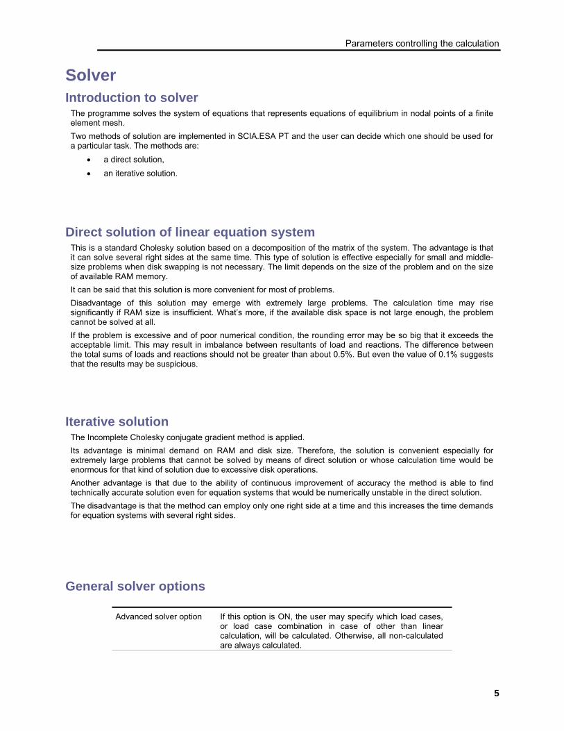
Displaying the natural frequencies The calculated eigenfrequencies (natural frequencies) may be displayed in summarised form in a preview table.

The procedure to display the table with eigenfrequencies 1. If it is not the case, perform dynamic calculation of the project. 2. Open service Results. 3. Double click function Eigenfrequencies

28

Dynamics

Displaying the eigenmodes The calculated eigenmodes may be displayed as any other result.

The procedure to see the modes on the screen 1. If it is not the case, perform dynamic calculation of the project. 2. Open service Results. 3. Select function Deformations of nodes. 4. Item Type of loads set to Mass combinations. 5. Item Value set to Deformed mesh. 6. In item Mass combination select the required eigenmode. 7. Press button [Redraw] to see the result.

29


Example

First five eigenmodes of a simple frame whose horizontal bar is subject to a distributed load are shown in the following pictures. Mass has been automatically generated from the load.

30

Nonlinearity Assumptions of non-linear calculation

The main difference between a linear and non-linear calculation is that the non-linear calculation gives such results of deflections and internal forces for which equilibrium conditions are satisfied on a deformed structure. The user should think beforehand whether the load applied on the structure would lead to such a state of deformation that affects the resultant internal forces and deflections. If the user thinks so, s/he should use the non-linear calculation at least for one selected load and compare the results with those for linear calculation. Thus, the user can evaluate the effect on non-linearity on behaviour of the structure. The non-linear calculation in SCIA.ESA PT is based on the following assumptions:

• equilibrium conditions are satisfied for deformed shape of a structure, • effect of axial forces on flexural stiffness of beams is taken into account as well, • non-linear supports are taken into consideration, • material of the structure is considered as linearly elastic.

The non-linear calculation is important especially for the following problems:

• suspended structures � e.g. rope systems, • slender members with imperfections and slender members taking account for buckling.

Note: Before a non-linear calculation can be carried out, the linear calculation MUST HAVE BEEN performed.

Nonlinearity options in setup If any kind of non-linearity should be taken into account in a project, it is necessary to select appropriate option (or options) in the Project data setup dialogue. The options related to nonlinearity are listed on tab Functionality. In order to make the options accessible, the main option Nonlinearity must be chosen. Once this is done, a list of options (or they may be called sub-options) is shown.

Initial deformation and curvature

This option enables the user to define an initial deformation of a structure.

2nd order - geometrical nonlinearity

This option enables the user to perform geometrically non-linear calculation of analysed structure.

Beam local nonlinearity This option provides for the introduction of local nonlinearities on individual beams.

Support nonlinearity If this option is ON, it is possible take account of nonlinearities in supports.

31


Solver options for non-linearity In addition to general parameters controlling the calculation, the non-linear calculation enables the user to define additional options.

Maximum iterations Specifies the number of iterations for the non-linear calculation. This value is taken into account only for the Newton-Raphson method. For the Timoshenko method, the number of iterations is automatically set to 2. The termination of calculation is controlled by means of convergence accuracy or by means of the given maximal number of iterations. If the limit is reached, the calculation is stopped. If this happens, it is up to the user to evaluate the obtained results and decide whether (i) the maximum number of iteration must be increased or whether (ii) the results may be accepted. For example, if the solution oscillates, the increased number of iterations won�t help.

Plastic hinge code If this option is ON, the non-linear calculation takes account of plastic hinges. It is possible to select the required national standard that will be used to reduce limit moments. If no standard is selected, no reduction is performed.

Geometrical nonlinearity If this option is ON, the second order effects are considered during the calculation. It is possible to select either Timoshenko or Newton-Raphson method. For both methods, the exact solution of beams is implemented. It takes account of normal forces and shear deformation for any kind of loading. Transformation of internal forces into the deformed beam axis is included.

Number of increments This parameter is applied for Newton-Raphson method only. Usually, one increment gives sufficient results. If deformation is large, the calculation issues a warning and the number of increments can be increased. The greater the value is, the longer it takes to complete the calculation.

The limits of the calculation are:

Total number of nodes and finite elements unlimited Total number of non-linear combinations 1000 Maximal number of iterations (in one increment) 999 Maximal number of increments 99

32

Nonlinearity

Initial stress options A beam of the analysed structure may be subject to an initial stress. This pre-stress may be defined in several ways: The approach can be adjusted in the Solver options setup dialogue.

Initial stress If ON, some initial stress will be defined. Initial stress as input If ON, the initial stress is specified by a fixed user-

input value. If OFF, see below.

Stress from load case The initial stress may be calculated automatically from the results of selected load case. The results of linear static calculation for the specified load cases are used to determine the initial stress in the beam.

Newton-Raphson method The algorithm is based on Newton-Raphson method for solution of non-linear problems. The method is robust for most of problems. It may, however, fail in the vicinity of inflection points of loading diagram. This may occur for example at compressed beams subject to small eccentricity or to small transverse load. Except for the mentioned example, the method can be applied for wide range of problems. It provides for solution of extremely large deformations. The load acting on the structure can be divided into several steps. The default number of steps is eight. If this number is not sufficient, the program issues a warning. The rotation achieved in one increment should not exceed 5°. The accuracy of the method can be increased through refinement of the finite element mesh or by the increase in total number of increments. For example, the solution of a single beam divided to a single finite element will not give sufficient results. In some specific cases, high number of increments may solve even problems that tend to a singular solution which is typical for the analysis of post-critical states.

Timoshenko method The algorithm is based on the exact Timoshenko�s solution of a beam. The axial force is assumed constant during the deformation. Therefore, the method is applicable for structures where the difference of axial force obtained by 1st order and 2nd order calculation is negligible (so called well defined structures). This is true mainly for frames, buildings, etc. for which the method is the most effective option. The method is applicable for structures where rotation does not exceed 8°. The method assumes small displacements, small rotations and small strains. If beams of the structure are in no contact with subsoil and simultaneously they do not form ribs of shells, no fine division of beams into finite elements is required. If the axial force is lower than the critical force, this solution is robust. The method needs only two steps, which leads to a great efficiency of the method.

The first step serves only for solution of axial force. The second step uses the determined axial forces for Timoshenko´s exact solution. The original Timoshenko´s solution was generalised in SCIA.ESA PT and the shear deformations can be taken into account.

33


Initial deformation and curvature Initial deformation and curvature

If required, an initial deformation of analysed structure can be introduced. There are various approaches in SCIA.ESA PT to do so.

None The structure is ideal without any imperfections. Simple inclination The imperfection is expressed in the form of a simple

inclination. The inclination may be defined in millimetres per a metre of height of the structure. It means that only horizontal inclination in the global X and Y direction may be specified. The inclination is linearly proportion to the height of the building. This option is applicable mainly for high-rise buildings. It has no or minimal influence on horizontal structures.

Inclination + curvature of beams If this option is selected, the initial deformation may be defined the same way as above PLUS the curvature of beams may be specified as well. The curvature is the same for all the beams in the structure.

Inclination functions The initial imperfection is defined by a function (or curve). The user inputs the curve by means of height-to-imperfection diagram. This option is applicable mainly for high-rise buildings. It has no or minimal influence on horizontal structures.

Functions + curvature of beams The initial imperfection is expressed as a sum of inclination function and curvature. It is analogous to option Inclination and curvature of beams.

Deformation from load case This option requires two-step calculation. First, a calculation for a required load case must be performed. The deformation due to this load case is then used as the initial imperfection for further calculation.

Buckling shape This option requires two-step calculation. First, a stability calculation must be performed. The calculated buckling shape is then used as the initial imperfection for further calculation.

Regardless of the approach, the initial imperfection can be defined for a non-linear combination only. It is one of the parameters that the user may define in the Non-linear combination manager.

34

Nonlinearity

Note 1: The calculated and displayed deformation is ALWAYS measured from the imperfect model, i.e. it does not represent the total deformation from the ideal shape, but the overall deformation from the imperfect shape.

Note 2: Calculations taking account of any type of imperfection are non-linear calculations and as that they are sensitive to the size of finite elements. Or to be precise, they are sensitive to the number of finite elements per a member. The user MUST remember that a division giving just one finite element per a beam is NOT sufficient and may give completely misleading results.

Simple inclination Simple inclination simply defines how much the structure is inclined to one side. The inclination is applicable to vertical structures only. It defines an inclination in horizontal direction per a unit of height. The inclination may be defined in the direction of global axes X and Y. As an example, let�s assume a vertical cantilever subject to vertical concentrated force. If no inclination is defined, the horizontal displacement is zero.

35


If, however, a simple inclination is input, the result is affected by this imperfection and the column�s horizontal displacement is non-zero.

Inclination and curvature of beams A simple inclination may be combined with an initial curvature of beams. It is also possible to define zero inclination and use only the curvature as a factor determining the initial imperfection. If specified, the inclination is considered the same way as if it is used as the only source of imperfection. The given curvature is considered for all the beams in the structure. In other words, all the beams are subject to the same initial curvature. The programme automatically determines which direction of curvature is critical and uses that direction for calculation. The curvature is taken into account in all beams in the structure regardless of their spatial orientation. Unlike the simple inclination, it therefore affects even horizontal beams.

36

Nonlinearity

Let�s assume a simply supported beam whose initial imperfection will be defined solely by means of the curvature. The beam is axially compressed by means of two concentrated forces.

If the curvature is adjusted to a non-zero value, the final vertical displacement of the beam is also non-zero � see the picture.

If, on the other hand, the curvature is not applied (i.e. is set to zero), the beam (which is ideally straight) remains straight even when subject to the pair of axially acting forces.

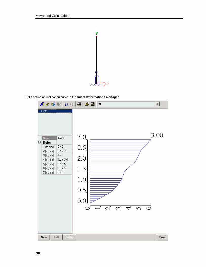
Inclination functions The inclination function may be considered similar to the simple inclination. It is applicable for vertical structures and it defines the horizontal inclination of the structure in the direction of global axes X and Y. The inclination function is defined by means of an inclination-to-height curve. The curve is than assigned to the appropriate non-linear combination. Let�s assume a single vertical column fixed at its foot. The column is subject to a vertical force.

37


Let�s define an inclination curve in the Initial deformations manager.

38

Nonlinearity

Let�s create a non-linear combination, adjust type of imperfection to Inclination function and select the previously defined curve.

The calculated horizontal displacement of the column will be affected by the imperfection.

Note: It must be emphasised here that the inclination function is defined in absolute co-ordinates, i.e. in co-ordinates of the global co-ordinate system. Therefore, in order to successfully introduce an inclination defined by an initial deformation curve, the user must ensure that the curve is defined at the level corresponding to global Z co-ordinates of the structure – see the table below.

The curve of Initial deformation is defined as above.

The curve is defined for the interval <0 � 3.0> (measured along the global Z axis).

Variant A The column foot is in the origin of the global co-ordinate system, i.e. its vertical co-ordinate is equal to 0.0 (zero).

The result is affected by the inclination curve.

39


Variant B The column foot is in the point whose global vertical co-ordinate is equal to 3.0.

The result is NOT affected by the inclination curve as the curve definition ends just at the foot of the column and therefore the column is not subject to any inclination.

Inclination function and curvature of beams The principle here is analogous to a simple inclination combined with a beam curvature. The only difference is that instead of a simple inclination expressed by a single number, the user can define a nonlinear inclination curve.

40

Nonlinearity

Deformation from load case Quite often it may happen that some of the loads are acting on a structure before any other load is imposed. In addition, it is possible that this initial load leads to significant imperfections that may considerably affect the static behaviour of the structure. A typical example is a rope structure, i.e. a structure whose parts are suspended on ropes or cables. Just the self-weight may cause a significant deflection of these ropes or cables. Also slender steel beams are a good example.

Example

Let�s consider a simply supported beam subject to two horizontal forces that compress the beam.

Let�s assume that the beam is slender and that just the weight of the material would cause a significant deflection. The first calculation is therefore made for "self-weight load case" only. Its results are shown below.

The obtained result (for the self-weight) can be then selected in the Non-linear combination manager as the source of the initial imperfection.

The final non-linear calculation then gives results taking account of the pre-deformation.

41


If the initial imperfection had not been taken into account at all in our sample structure, the results would have been completely different. The beam, ideally straight and subject to axial load only, would show no deformation perpendicular to the longitudinal axis.

Note: Usually (but not exclusively), a static linear calculation is sufficient enough for the determination of the initial imperfection due to a specific load case. Subsequent calculation whose aim is to take account of the initial imperfection, however, must already be a non-linear one.

Note: The calculated and displayed deformation is ALWAYS measured from the imperfect model, i.e. it does not represent the total deformation from the ideal shape, but the overall deformation from the imperfect shape.

Beam non-linearity Beam local nonlinearity

The term Beam local nonlinearity covers phenomena related to a non-linear behaviour of individual beams. In SCIA.ESA PT beams may be of four types:

Standard This beam type is not subject to any kind of non-linearity.

Tension only Beam of this type is capable of transferring only tension forces. The beam is indefinitely weak under compression. Only tensile axial force may occur in this beam type.

Compression only Beam of this type is capable of transferring only compression forces. The beam is indefinitely weak

42

Nonlinearity

(called also Press only) under tension. Only compressive axial force may occur in this beam type.

Initial stress A non-zero initial stress is defined in a beam. The stress is constant along the whole beam.

Note 1: If the above-mentioned phenomena should be taken into account in a calculation, a non-linear calculation must be performed. If only a static linear calculation is carried out, any possibly defined non-linearity in any of beams is not taken into account and the results are the same as for standard beams.

Note 2: A non-linear calculation can be performed ONLY for a non-linear combination. Therefore, it is necessary to define such combination or combinations prior to the start of a non-linear calculation.

Compression-only beams The compression-only property can be adjusted in a property table of a particular beam.

The effect of this option will be shown on the following example. Let�s assume a simple two-span frame whose horizontal beams must be, for some reason or another, supported during the assembly phase by props.

43


Further, let�s assume that the frame is subject to two load cases during this assembly phase. The first one represents a uniform distributed load acting on both spans.

The other one contains a uniform distributed load on the right hand side span only.

You may have noticed the mark on the props. The pair of double arrows indicates that the beam is of compression-only type.

44

Nonlinearity

A non-linear calculation can only be performed for a non-linear combination even if the combination should contain just one load case. Therefore, let�s define two non-linear combinations, one for the two-span load and one for the one-span load.

Let�s carry out non-linear calculation (do not forget to select solver option Beam nonlinearity). The following figures show results for the two loads.

45


Axial force in beams for the two-span load.

Axial force in beams for the one-span load.

Notice that there is no axial force in the left prop. The prop would get under tension if standard beams would be used for the whole structure. But as we defined the props as compression-only, the calculation removes the prop from the model once it finds that it gets under tension.

Deformation of the frame for the one-span load.

46

Nonlinearity

In this detail look you may clearly see that the horizontal beam is torn away from the top end of the prop.

Comparison with static linear calculation

The following set of pictures demonstrates what would have happened if just a linear calculation had been performed.


This result is identical to the result of non-linear calculation for the first combination (the two-span load combination). In this load case both props are under compression. There is no need to take any corrective measures and therefore, the result of linear and non-linear calculation is identical.

47



Axial force in beams for the two-span load in detail.

For the second load case representing the load acting on the right hand side span only, the situation is different. The left prop gets under tension and there is a tensile axial force in it.

Also the diagram of displacement shows that the prop remains "connected" to the horizontal beam, "holds" it firmly and influences the overall deformation of the frame.

48

Nonlinearity

Tension-only beams The principle of tension-only beams is analogous to compression-only beams.

Let’s explain the principle on a simply supported beam with an overhanging load. Further, let’s assume that for some reason the vertical deflection of the free end must be limited. Therefore, a suspension cable is attached to the free end. The suspension cable will not prevent the beam end from "going up", but will significantly reduce any possible downward vertical deflection. Such a type of beam can be successfully modelled by means of a tension-only beam.

Our example will compare two variants: (i) one with the suspension rope, and (ii) one without it. Similarly to compression-only beams, a special symbol is drawn on the tension-only beam. A pair of double-arrows whose tips point in opposite direction and away from each other forms the symbol.

49


Let�s define load that will help us show the difference between the two variants. The first load case represents a vertical concentrated force located in the middle of the span between the supports.

The second load case contains a vertical concentrated force located in the middle of the free "overhanging" end.

50

Nonlinearity

Let�s carry out a non-linear calculation with option Beam nonlinearity ON. The results for the first load case will be identical for both variants: the suspension cable does not act and therefore does not affect the behaviour of the structure.

On the other hand, the results for the second load case are different. The vertical deflection of the free end for the "suspended" variant is significantly smaller than for the "non-suspended" variant.

51


Initial stress in beams Sometimes, it may be required to analyse a structure that is subject to some pre-stressing. SCIA.ESA PT enables the user to define an initial stress in a beam. The initial stress may differ from beam to beam and is always considered constant along one particular beam. The application is demonstrated on a following example. The definition of an initial stress is made in a similar way as the compression-only property is adjusted for compression-only beams.

52

Nonlinearity

Let�s assume a simply supported beam with two pinned ends.

The first (top most) beam is a standard beam without any initial stress defined. The second (the middle) one is subject to a compression axial force of 50kN (i.e. �50 kN). The third (bottom most) beam is subject to a tensile axial force of 50kN (i.e. +50 kN). All the variants are subject to the same external load: a vertical concentrated force. The definition may be easily verified on diagrams of calculated axial force.

53


The last set of pictures then shows the effect of the initial stress on vertical displacement. The beam subject to an initial compression shows the biggest deformation.

Support non-linearity Support non-linearity

A support may be of various properties concerning its action. SCIA.ESA PT offers both standard and, let�s say, advanced types of supports. Concerning translation (displacement) in a specific direction a support may be:

free There is no constrained applied in the specific direction.

rigid The member is fully fixed in the specific direction. flexible A spring may be assumed in the specific direction.

Stiffness must be specified for this support type. rigid press only This type is capable of action only if there is

compression in the support. The support is rigid when under compression. Under tension, the support is free-like.

flexible press only This type is capable of action only if there is compression in the support. The support is of specified stiffness when under compression. Under tension, the support is free-like.

54

Nonlinearity

Concerning rotation around a specific axis a support may be:

free There is no constrained applied around the specific axis.

rigid The member is fully fixed concerning rotation around the specific axis.

flexible A spring may be assumed to hold the rotation around the specific axis. Stiffness of the auxiliary spring must be specified for this support type.

Note 1: If the above-mentioned phenomena should be taken into account in a calculation, a non-linear calculation must be performed. If only a static linear calculation is carried out, any possibly defined non-linearity in any of supports is not taken into account and the results are the same as for standard supports.

Note 2: A non-linear calculation can be performed ONLY for a non-linear combination. Therefore, it is necessary to define such combination or combinations prior to the start of a non-linear calculation.

Flexible support For any of directions in which a support acts, it is possible to define a specific flexibility (or stiffness) of the support. To do so, a standard support must be defined and the required constraint set to "flexible". This may be done in the property table of the support.

Let�s assume a cantilever beam subject to a concentrated force load acting at the free end.

55


The support is defined as flexible in rotation. The flexibility of the support is set to (seen from the top) (i) 1 MNm/rad, (ii) 5 MNm/rad, (iii) complete rigid fixing. The following picture shows the effect of the stiffness on the vertical displacement of the cantilever beam.

Note: This type of analysis does not required non-linear calculation. The static linear calculation is sufficient to give correct results.

56

Nonlinearity

Rigid compression-only support This type of support gives a full support (fixing) when under compression. If there is a tension in this type of support, the support ceases to give any support and is "absenting" from the model. Let�s assume a simply supported beam with an additional intermediate support (intentionally we do not speak about continuous beam in this context). The intermediate support is of discussed compression-only type. As a result, the support acts only if some load is applied in downward direction.

First, let�s apply a vertical load acting in downward direction.

Second, let�s apply a vertical load acting in the opposite, i.e. upward, direction.

57


The following set of pictures shows the results for individual loads. Diagrams of reactions and deformation are shown.

58

Nonlinearity

Flexible compression-only support This type of support gives a partial support (behaving like a spring) when under compression. If there is a tension in this type of support, the support ceases to give any support and is "absenting" from the model. Let�s, as in chapter Rigid compression-only support, assume a simply supported beam with an additional intermediate support The intermediate support is of discussed flexible-compression-only type. As a result, the support acts only if some load is applied in downward direction. For better understanding, the results are compared with the results of example analysed in chapter Rigid compression-only support. The intermediate support of the top beam is of Flexible compression-only type. The intermediate support of the bottom beam is of Rigid compression-only type.

The first comparison shows vertical displacement for load acting in vertical downward direction. It can be seen that the flexible support provides for a partial vertical displacement.

59


The second comparison shows vertical displacement for load acting in vertical upward direction. It proves that none of the two intermediate supports is "active" when tension appears in it.

Second order calculations Sample analysis - guyed mast

Structure

A mast with three guy ropes. A steel tubular section has been used for a column shaft. Ropes are modelled as steel bars with a sectional area equal to the sectional area of the rope. The structure is subject to dead load and to the effect of wind.

60

Nonlinearity

The load scheme is in the picture below.

Aim of the analysis

The aim is to examine a deformation shape and internal forces for the given load conditions.

Analysis

It is quite obvious that horizontal stiffness of such a structure depends on stiffness of the ropes. In order to calculate with realistic rope stiffness, a deflection of ropes due to their self-weight must be included into the analysis. A slacked rope has significantly lower stiffness than a straight rope (e.g. a rope lying on a flat pad or a rope hanging vertically). Therefore, a full attention should be paid to proper modelling of the ropes with regard to their �slackness� (self-weigh deflection).

61


The �slackness� of ropes, of course, depends on their pre-stressing. The problem of guessing the proper pre-stressing may be an iterative process based mainly on engineer�s experience. The pre-stressing in our example has been introduced by means of temperature load � see the figure below.

A fine finite element mesh has been used to obtain high quality results with respect to the deflection of ropes. The calculation of axial forces representing the pre-stressing due to thermal load has been carried out as linear calculation. The following picture shows the resultant axial forces.

Let�s use these axial forces as the pre-stressing and use them for a successive calculation for the dead load. In other word, let�s start non-linear calculation with the pre-stressing taken into account.

62

Nonlinearity

Note: This calculation procedure corresponds with the following idea about a construction process. First, the structure is assembled in a state of weightlessness and is pre-stressed in this state. Then the structure is subject to the effect of gravity.

The deformation shape and axial force diagram is shown in the following figure. The axial forces are the sum of axial forces produced by pre-stressing and axial forces due to self-weight.

As a next step, the wind calculation has been performed. �Tightening� of ropes on the windward side results in increased stiffness of the ropes on that side and simultaneous slacking of the ropes on the leeward side leads to dramatically decreased stiffness of the ropes there. The superposition principle cannot be applied in the non-linear analysis. Therefore, the effect of the self-weight and the wind cannot be analysed separately and then combined in the postprocessor. A combination must be created in advance and the calculation must be carried out for this non-linear combination. The resultant deformation shape is brought in the picture below.

63


And the next figure shows distribution of the axial force.

64

Nonlinearity

Below there is another view of axial force diagrams.

65

Linear buckling Assumptions of linear buckling calculation

The word �linear� suggests that the following phenomena cannot be taken into account: • non-linear elastic supports and foundation, • beams acting in compression or in tension only.

Since the calculation is linear, both types of non-linearity listed above are considered in a way that corresponds to equilibrium equations assembled on a non-deformed structure. In other words, foundation stiffness is equal to stiffness for zero deflection and �one-way-action� beams are taken as usual beams. Let�s start with the equilibrium equation

(KE + KG) u = R

where KG is a geometric stiffness matrix reflecting the effect of axial forces in beams and slabs.

The basic assumption is that the elements of the matrix KG are linear functions of axial forces in beams. That

means, matrix KG corresponding to a K-th multiple of axial forces in the structure is the K-th multiple of original matrix KG. The aim of the buckling calculation is to work out such a multiple K for which the structure loses stability. Such a state happens when the equation below has a non-zero solution.

(KE + K . KG) u = 0

In other words, such a value K should be found for which the determinant of the total stiffness matrix (the term in the brackets) is equal to zero. Like for the natural vibration analysis the subspace iteration is used here. Similarly to the dynamic calculation also here the result is a series of eigenmodes and corresponding K -multiples. The first

eigenmode is usually the most important and corresponds to the lowest K -multiple. A possible collapse of the structure usually happens for this first mode. Note: There is a difference in behaviour of beam and shell elements. For shell elements the axial force is not considered in one direction only. The shell element can be in compression in one direction and simultaneously in tension in the perpendicular direction. Consequently, the element tends to buckle in one direction but is being �stiffened� in the other direction. This is the reason for significant post-critical bearing capacity of such structures. The calculated buckling eigenmodes can help the structural engineer to get an idea about behaviour of a structure and about possible mechanisms of buckling failure. The resultant critical multiple suggests how far the structure is from possible buckling.

Sample analysis - column Similarly to dynamics, calculation of buckling depends on the finite element mesh. The effect of mesh density will be demonstrated on an analysis of a frame column that is supported in a horizontal direction by wind stiffeners at the floor levels (see figure).

67


The supposed shape of buckling is in the following figure.

If the usual mesh size, i.e. one finite element per one beam, is used, the model has no degrees of freedom for horizontal translations in the middle of heights of individual floors, which prevents the buckling. Because, however, rotations in floor levels are not constrained even such a poor model would eventually buckle. But, the result would show a significant numerical error. The coarse division (one element per a floor) gives the critical multiple that is equal to 213, while a variant with nodes in the middle of the heights gives the multiple of 163. It is definitely clear that the difference is not negligible. The following pictures demonstrate the above said facts. They also show that once an FE node is in the middle of the floor, further refinement of the mesh gives only small improvement in results.

68

Linear buckling

4 finite elements per column, i.e. 1 FE per floor critical multiple = 213

8 finite elements per column, i.e. 2 FEs per floor critical multiple = 163

69


10 finite elements per column critical multiple = 161

50 finite elements per column critical multiple = 160

70

Index B

buckling....................................................................67

C

calculation parameters..... 3, 5, 6, 8, 11, 13, 17, 31, 32, 34, 35, 36, 37, 40, 41, 42, 43, 49, 52, 54, 55, 57, 59, 67

D

dynamics ................................ 8, 21, 23, 24, 25, 28, 29

F

FE mesh .............................................3, 11, 13, 17, 67

foundation ................................................................17

free vibration............................................................25

H

haunch................................................................11, 13

I

Initial stress options .................................................33

M

masses................................................................ 23, 24

mesh......................................................... 3, 11, 13, 17

N

Newton-Raphson method ........................................ 33

nonlinearity....8, 31, 32, 34, 35, 36, 37, 40, 41, 42, 43, 49, 52, 54, 55, 57, 59, 60

S

solver ........................................................... 5, 6, 8, 25

support ......................................................... 54, 57, 59

T

Timoshenko method ................................................ 33

W

Welcome.................................................................... 1

71

scia.esa pt - nemetschek calculations... · scia.esa pt advanced calculations . ... • non-linear...

Documents