Gjsn Fyqfdubujpot boe Jowftunfou; Fwjefodf gspn uif Dijob-Kbqbo JtmboeEjtqvuf

Difoh Difo, Ubutvsp Tfohb, Diboh Tvo boe Ipohzpoh [iboh

Working Paper No. 949 Pdupcfs 3128 JTTO 2584-1389

School of Economics and Finance

Firm Expectations and Investment: Evidencefrom the China-Japan Island Dispute∗

Cheng Chen† Tatsuro Senga‡ Chang Sun§ Hongyong Zhang¶

October 14, 2017

Abstract

How do real-time expectations affect firms’ economic decisions? We provideevidence by using a dataset on Japanese multinational firms’ sales forecasts andexploring an unexpected escalation of a territorial dispute between China andJapan in 2012. Our estimation substantiates that, after the escalation of the dis-pute, affiliates of Japanese multinational firms in China experienced a sharp buttemporary decline in total sales relative to affiliates in other countries and a morepersistent decline in investment. Moreover, the territorial dispute has led to persis-tent pessimism in these firms’ expectations about future sales, which can explain60% of the overall decline in investment.JEL: E22, E32, D84, F51.Keywords: forecasts, pessimistic expectations, geopolitical events, investment.

∗This research was conducted as a part of the Project “Data Management” at the Research Instituteof Economy, Trade and Industry (RIETI). We are grateful to Pol Antràs, Nick Bloom, Steven Davis, TaijiFurusawa, Tomohiko Inui, Arata Ito, Keiko Ito, Yulei Luo, Masayuki Morikawa, Liugang Sheng, Zhi-gang Tao, Makoto Yano and seminar participants at CUHK, RIETI, SED, Stanford and Purdue (Midwesttrade conference) for their helpful comments. Financial support from the University of Hong Kong,Hong Kong General Research Fund (project code: 17507916), and RIETI is greatly appreciated.

†University of Hong Kong. Email: ccfour@hku.hk.‡Queen Mary University of London and RIETI. Email: t.senga@qmul.ac.uk.§University of Hong Kong. Email: sunc@hku.hk.¶RIETI. Email: zhang-hong-yong@rieti.go.jp.

1. Introduction

Unexpected demand or supply shocks can affect firms’ performance as well as expec-tations. Many important decisions rely heavily on firms’ expectations about futuredemand and supply conditions. A burgeoning literature investigates how economicagents form expectations and how these expectations evolve over the business cycle(Coibion and Gorodnichenko 2012, 2015; Bachmann et al. 2013, 2017; Coibion et al.2015; Kozlowski et al. 2015; Orlik and Veldkamp 2015). However, there is little evi-dence on how real-time expectations of firms affect their economic decisions, includingprice-setting, hiring and investment. Understanding the relationship between shocks,expectations and firm-level decisions is crucial for the study of macroeconomics.

There are two main challenges to identifying the impact of expectations on firms’economic decisions. First, such an analysis requires panel data on firms includingboth realized and forecasted value of variables such as sales and investment. Second,we need exogenous and unexpected shocks that can change firms’ performance andexpectations. We address these two challenges by using a unique (panel) dataset ofJapanese multinational firms that contains firms’ forecasts for future sales and explor-ing the effect of an unexpected escalation of a territorial dispute between China andJapan in 2012. In particular, we examine how the unexpected shock led to a decline inaffiliates’ investment by changing these firms’ expectations.

China and Japan experienced an escalation of a serious territorial dispute in thethird quarter of 2012. The two countries have been disputing over the sovereignty ofthe uninhabited Senkaku Islands (also known as Diaoyu Islands) for years. In August2012, the Japanese government announced its consideration of purchasing the islandsfrom the private owner in Japan, which triggered anger in China and led to a firstwave of anti-Japanese protests in August and a second wave of protests in more than180 Chinese cities in September. It was reported that the sudden crisis (henceforth,“Island Crisis”) negatively impacted Japanese multinational firms’ operation in Chinaas well as their expectations about future sales.1 Using affiliates in other countries as acontrol group, we estimate the causal impact of the Island Crisis on firms’ expectationsand investment. Using additional identification assumptions, we identify the effect offirms’ expectations on their investment.

We document three facts regarding the impact of the Island Crisis using difference-in-differences (DID) strategies. First, sales of Japanese affiliates in China dropped forthe year of 2012, but recovered within two years, relative to sales of affiliates in othercountries. Second, capital investment of affiliates in China dropped in 2012 and it didnot show any sign of recovery as of 2014, the last year in our dataset. The largestimpact on investment appeared in fiscal year of 2014, two and a half years after the

1A firm-level survey on Sino-Japan relationship done by Teikoku data bank in October 2012 showedthis trend. For details (in Japanese), see Teikoku Data Bank (2012) or http://www.tdb-di.com/visitors/kako/1210/summary_2.cgi.

1

Island Crisis.2 Third, we find that the expectations of affiliates in China became morepessimistic after the Island Crisis compared to affiliates in other countries. To showthis, we construct a measure of forecast errors (FEs), defined as the percentage devi-ation of the realized sales (one year later) from the (current) forecast for next year’ssales. The Island Crisis induced a persistent increase in this measure for 2012 and2013, which suggests that affiliates in China continued to be pessimistic at least until2013, though sales had already recovered at this point.

These three facts point to a belief-driven mechanism through which the unex-pected, temporary shock continues to affect firms’ investment. To quantify how muchof the induced decline in investment was caused by pessimistic expectations, we pro-ceed in two steps. First, we made an additional assumption that the Island Crisis isuncorrelated with determinants of investment other than firms’ expected sales, con-ditioning on a set of fixed effects and firm characteristics that include existing capitalstock, liquidity and firm age. Based on this assumption, we use the Island Crisis as aninstrumental variable (IV) to estimate the effect of firms’ expected sales on investment.The elasticity of investment with respect to sales forecasts is around 1.65 in the shortrun (i.e., one year) and round 1.93 in the medium run (i.e., two years). Second, weperform a simple back-of-the-envelope calculation with the following thought exper-iment: had Japanese affiliates in China not been pessimistic (i.e., zero FEs on averageafter the crisis), that is, had they predicted the average sales in 2013, how much less ofa decline in investment would there be? Our DID regressions show that the Island Cri-sis made Japanese firms’ investment in China drop by roughly 13.7% (and 15.8%) andtheir sales forecasts drop by roughly 5.4% (and 4.8%) in one year (and in two years).Therefore, the pessimism due to the Island Crisis explains roughly 60% of the overalldrop in Japanese affiliates’ investment in China after the crisis, which is quantitativelysignificant.

Our paper contributes to a growing literature that uses forecasting data to analyzeeconomic agents’ beliefs and how the beliefs evolve over business cycles (Coibion andGorodnichenko 2012, 2015; Bachmann et al. 2013, 2017; Coibion et al. 2015; Kozlowskiet al. 2015; Orlik and Veldkamp 2015). As Coibion et al. (2017) pointed out, thereis a lack of empirical evidence on how real-time beliefs of firms affect their economicdecisions. We are among the first to use a firm-level panel dataset that contains real-ized and forecasted values of firm sales across periods to explore this important issue.Moreover, using the Island Crisis as an exogenous shock helps to address some iden-tification issues when using other types of shocks such as aggregate movement overbusiness cycles.3

2In our data, the fiscal year starts on April 1 of each year and ends on March 31 of the next year.3Bachmann et al. (2017) used survey data from Ifo on firm investment expectations and realizations

to build a panel dataset of investment expectation errors and analyzed time series and cross-sectionalfeatures of these errors. Our paper differs from Bachmann et al. (2017) in that we look at sales fore-casts that they do not have in their data. We also investigate how an unexpected geopolitical shockaffected firm investment via influencing firm’s forecasts, which is not the research question addressed

2

Our paper is related to the literature on uncertainty and firm behavior. Previ-ous research has extensively investigated how objective uncertainty in aggregate orfirm-level variables evolves over business cycles and how it affects firm investment.4

Some recent papers focus on subjective measures of firms’ uncertainty (see, for exam-ple, Guiso and Parigi, 1999; Bachmann et al. 2013; Morikawa 2013, 2016; Senga 2017).Though our analysis does not involve uncertainty directly, the finding that sales andforecasts are impacted differently by the aggregate shock suggests that it may be im-portant to distinguish between objective and subjective uncertainty in business cyclestudies.

This paper finds that a change in firms’ expectations due to a short-lived shockplays an important role in generating a persistent impact on medium- to long-runeconomic activities such as firm investment. This has not been documented muchin previous studies that examine effects of sudden and short-lived events. For in-stance, event studies in international trade fail to find long-run impacts of suddenevents on trade-related variables (e.g., Fuchs and Klann 2013; Boehm et al. 2015). Onthe contrary, our paper finds a long-run negative impact of a geopolitical conflict oninvestment by multinational corporations (MNCs). This finding points out an impor-tant channel through which sudden events can affect firm behavior in the medium tolong run through their beliefs. This in turn has long-lasting effects on real economicactivities, a similar point made by Kozlowski et al. (2015) in their study of businesscycles.

The rest of the paper is organized as follows. Section 2 describes the escalation ofthe Island Crisis. Section 3 presents our empirical results, starting with some stylizedfacts, followed by DID estimation. Section 4 concludes.

2. The Island Crisis

China and Japan have been debating over the sovereignty of the Senkaku islands (alsoknown as Diaoyu Islands) for years, and the most serious conflict over the islands be-tween between the two countries by far happened in the third quarter of 2012. OnJuly 7, Japanese Prime Minister Yoshihiko Noda expressed his consideration for theJapanese government to buy the disputed islands, which triggered a wave of anti-Japanese protests in several Chinese cities on August 19th. On September 10th, the

by Bachmann et al. (2017).4Various theories have been proposed to explain why uncertainty varies over time and how it ad-

versely affects firm investment. For example, existing theories have shown that increased uncertaintyraises the option value of waiting in the presence of nonconvex adjustment costs (Bernanke 1983; Dixitand Pindyck 1994; Abel and Eberly 1996; Bloom 2009), which makes firms delay their investment. Bakerand Bloom (2013) use natural disasters as experiments to investigate the relationship between uncer-tainty and growth. For empirical measures of uncertainty, several candidates have been proposed,including stock-price volatility (Leahy and Whited 1996), the frequency of appearance of words such as“uncertain” in news articles (Baker et al. 2016), and disagreement among forecasters (Backmann et al.2013). These proxies are used to show that investment is negatively associated with uncertainty at thefirm level. See Bloom (2014) for a literature review.

3

Japanese government announced that it had decided to purchase the disputed islandsfrom a private Japanese owner in an effort, Tokyo claimed, aimed at diffusing territo-rial tensions. However, much larger scale anti-Japanese demonstrations subsequentlyoccurred. During the weekend of September 15-16, citizens in mainland China partic-ipated in protest marches and called for a boycott of Japanese products in as many as85 Chinese cities. Moreover, on September 18th, people in over 180 Chinese cities at-tended protests against Japan on the 81st anniversary of the Mukden Incident, whichwas seen as the start of the Japanese invasion of Manchuria in Northeast China.

The severity of this territorial dispute was unprecedented, and it was unexpectedby Japanese firms in China. The anti-Japanese movements between August and Septem-ber of 2012 had generated significant impact on Sino-Japan economic relations. AsFigure 1 shows, the share of manufacturing FDI flows from Japan in China’s totalmanufacturing FDI inflows plummeted from 22% (the third quarter of 2012) to 9%(the third quarter of 2014) in two years. One survey done by Teikoku Databank in Oc-tober 2012. showed that the sudden escalation of the island dispute was unexpectedby Japanese firms, and one third of firms surveyed thought that the unexpected anti-Japanese demonstrations would negatively affect their sales in China.5 Moreover, onesixth of them planned to withdraw or reduce their investment in China.6 The IslandCrisis could have affected both demand- and supply-side factors among Japanese affil-iates in China. On the one hand, Chinese consumers boycotted Japanese goods duringthe crisis. Even consumers who like Japanese products might be afraid of being seenas unpatriotic or having their possessions being destroyed.7 On the other hand, an-gry protestors ransacked Japanese stores and plants, which we see as supply shocksto Japanese affiliates. We do not try to distinguish between demand- and supply-sideshocks in this paper. Our estimates of the impact of the Island Crisis on sales, invest-ment and sales forecasts could operate through both demand and supply conditionsamong firms.

3. Empirical Findings: Differences-in-Differences Estimation

3.1. Data Description

We use the parent-affiliate-level data of the Basic Survey of Overseas Business Activ-ities (BSOBA, Kaigai Jigyo Katsudo Kihon Chosa) prepared by the Ministry of Econ-omy, Trade and Industry (METI). This survey covers two types of overseas subsidiaries

5For details, see Teikoku Data Bank (2012) or http://www.tdb-di.com/visitors/kako/1210/summary_2.cgi, both of which are in Japanese.

6It was reported that the substantial scale-up of anti-Japan protests was related to problems associ-ated with the transition of political power in China around the same time. This further shows that theescalation of the island dispute was exogenous to other demand and supply conditions of Japanese affil-iates in China. For details, see http://www.cnn.com/2012/09/18/world/asia/china-protests-japan-fury/index.html.

7Bradsher (2012) reported that in Xi’an, China, a man who was driving a Toyota Corolla was severelybeaten by the anti-Japanese protestors while the car was destroyed.

4

of Japanese MNCs: (1) direct subsidiaries with ratios of investment by Japanese enter-prises’ being 10% or higher as of the end of the fiscal year (March 31), (2) second-generation subsidiaries with the ratio of investment by Japanese subsidiaries of 50%or higher as of the end of the fiscal year (March 31). This survey is conducted annuallyvia a questionnaire based on self-declaration survey forms (one for the parent firmand another one for each foreign affiliate) sent to the parent firm in the beginning ofthe next fiscal year. The survey form for parent firms includes variables concerningthe parent’s sales, capital, employment, industry classification, etc. The survey formfor the foreign affiliates reports their equity, sales, investment, number of employees,country and industry information, the date of establishment, and operation status in-cluding dissolution or withdrawal.

Based on this annual survey, we constructed a panel dataset of foreign affiliatesfrom 2007 to 2014 that includes both manufacturing and non-manufacturing firms.Each parent-affiliate pair is traced throughout the period using an identification code.To obtain real sales and investment, we deflate parents’ and affiliates’ sales and invest-ment using the GDP deflator for Japan and that of each country in which an affiliateis located, respectively. Summary statistics of this dataset are reported in Table 1; andthe total number of observations across 8 years is roughly 170,000.

We constructed the variable of capital stock at the affiliate level as part of the study,as the data do not contain information on capital. As the time span of our data is notlong, we cannot use the perpetual inventory method. Instead, we use investment in-formation and equity information in the first year when the firm appears in the datato construct firm’s capital stock. Specifically, the capital stock at year t is calculatedas Kt = 0.9 ∗ Kt−1 + invt, where Kt−1 is the capital stock in year t − 1 and invt is theinvestment made in year t. For the first year when the firm appears in the data, weuse the registered equity to proxy for its initial capital. As some of our regressions usethe investment ratio and the ratio of liquidity to capital stock, we also construct suchvariables by dividing the amount of investment and cumulative retained earnings bythe capital stock. As there are outliers in the calculated investment ratio and the cal-culated ratio of liquidity to capital stock, we trim observations that are among the topor bottom one percent of these variables.

Important for our study, Japanese foreign affiliates report both the realized andthe projected value of total sales. These variables allow us to calculate forecast errors(FEs) for each affiliate in each year. Specifically, sales FEs are defined as the percentagedeviation of realized sales from the projected sales made one year earlier:

FEt =Salest

Et−1(Salest)− 1.

Therefore, if the firm underpredicts its sales, the forecast error defined above will bepositive, and negative when the firm overpredicts its sales. To exclude extreme values,we trimmed observations that are among the top or bottom one percent of FEt.

5

In the fourth row of Table 1, we present summary statistics for these FEs. Theaverage is 0.4%, a number very close to zero. This variable varies from a minimum of−85% to a maximum of 207%, and the standard deviation is roughly 29%. We furtherplot the distribution of FEt in Figure 2. The graph confirms that FEs are centeredaround zero. Therefore, firms sometimes overpredict and sometimes underpredicttheir sales. But on average, they are able to predict their sales next year quite precisely.

Because there are a reasonable number of observations (43%) in our data that donot include forecasts, we show that the existence of such observations should not af-fect our empirical findings. First, Figures 3 and 4 present the employment and salesdistribution of observations that report sales forecasts and of those that don’t report.It is straightforward to observe that the two distributions are similar. In particular, themean and variance of the two distributions do not differ in the statistical sense. More-over, these features hold for Japanese affiliates in China as well, as shown by Figures 5and 6. In total, we conclude that the existence of observations that did not report theirsales forecasts should not affect our empirical findings.8

3.2. Empirical Findings

In this section, we empirically explore how the Island Crisis in the third quarter of 2012affected Japanese multinational firms in China. Our findings are summarized by thefollowing four points. First, total sales of Japanese affiliates in China dropped sharplybut not persistently. Second, capital investment of Japanese affiliates in China beganto drop substantially and persistently after the Island Crisis. Third, Japanese MNCs inChina kept generating positive FEs of total sales after the Island Crisis. That is, evenafter their total sales rebounded, they kept underestimating total sales. Finally, lowlevels of forecasts (i.e., positive FEs) caused by the Island Crisis generated a negativeand quantitatively sizable impact on firm-level investment, accounting for roughly60% of the overall drop in aggregate investment after the Island Crisis. Since we wantto tease out shocks common to all Japanese affiliates abroad, we implement DID re-gressions and add country-specific time trends (i.e., China and non-China) into ourregressions. DID analysis suggests that the year of 2012 is indeed a turning point forJapanese MNCs’ affiliates in China, and we point out a potential explanation for thesedocumented facts: a relationship between subjective uncertainty and investment.

3.2.1. Finding One: Significant and Non-persistent Impact on Total Sales ofJapanese Firms in China

In this subsection, we present evidence that total sales of Japanese affiliates in Chinafell sharply but not persistently after the outbreak of the Island Crisis.9 Figure 7 shows

8Although simple regression analysis does show that larger firms are more likely to report salesforecasts, we do control for firm size (i.e., employment and/or sales) in our regressions when we lookat forecasts and FEs.

9We choose to focus on total sales instead of local sales for three reasons. First, our forecast data arefor total sales. We can make a meaningful comparison only by using both the projected and realized

6

that average annual growth rate of total sales did fall substantially in 2012 (i.e., com-pared to 2011), although it recovered substantially in 2013 and 2014. Moreover, a sim-ple plot of average sales in Figure 8 shows that Japanese affiliates in China suffered abig loss in sales in 2012 (compared to Japanese affiliates in other countries), while therecovery of their average sales was also substantial in 2013 and 2014. In addition, thefigure shows that the time trend of average sales in China is roughly the same as inother countries.

In order to confirm our finding for total sales, we run DID regressions by compar-ing total sales of Japanese affiliates in China to those in other countries after the IslandCrisis. Specifically, we run10

log(total sales) f t = β0 + β1Shockt ∗ China f + β2 ln(age) f t + β3 ln(equity)p( f )t

+β4 ln(sales)p( f )t + yeart + controlsj( f )t + f irm f + ε f t, (1)

where f represents the firm, and t and j denote the year and the country where theaffiliate is located, respectively. Subscript p( f ) is the ID of the parental firm of affiliatef . The dummy variable Shockt takes a value of one, if the year is later than or equalto 2012 and zero otherwise. The dummy variable China f equals one, if the affiliateis located in China and zero otherwise. Country-level control variables (controlsj( f )t)include log(GDP), log(GDP per capita) and annual GDP growth rate. In some of theregressions, we also control for (the logarithm of) affiliate’s employment. Finally, stan-dard errors are clustered at the country level, and China and non-China specific timetrends are included in the regression.

In order to check whether there are pre-trends for total sales of Japanese affiliates inChina, we implement a placebo test. Specifically, we move the timing of the shock to2009, 2010 and 2011 hypothetically and rerun the above regression. Moreover, in orderto detect the long-run impact of the Island Crisis on the total sales, we interact yeardummies after 2012 (i.e., yr2012, yr2013, yr2014) with the dummy variable that indicateswhether the affiliate is located in China (i.e., China f ) in some regressions (instead ofusing the shock dummy, Shockt).

Empirical results for how the Island Crisis affected total sales of Japanese affiliatesin China are reported in Tables 2 and 3. When we set the shock dummy to the year2009 or 2010, no significantly negative effect on Japanese affiliates in China is detectedby our DID regression (see columns (1), (2), (5) and (6)). However, when we set theshock dummy to the year 2011 or 2012, total sales of Japanese firms in China do seemto drop (relative to those in other countries) at least after we control for affiliate-level

total sales of Japanese firms. Second, we believe that the Island Crisis triggered both demand andsupply shocks to Japanese affiliates in China. Therefore, exports back to Japan and to other countrieswere also affected by the crisis and should be taken into account. Finally, although most firms reportannual total sales, there are substantially fewer firms that report annual local sales. We would lose 1/3of our observations if we used local sales instead of total sales.

10Note that the shock dummy, Shockt, is absorbed by the year fixed effects.

7

employment (see columns (3), (4), (7) and (8)). These findings suggest that total salesof Japanese affiliates in China probably already began to fall prior to the Island Crisis,which substantiates the existence of pre-trends for total sales. When we look at the per-sistency of the drop in total sales in China, Table 3 shows that the drop was significantonly in the year when the crisis happened (i.e., 2012) after we control for affiliate-levelemployment. This is consistent with the findings in Figure 7 and 8. Taken together,we conclude that total sales among Japanese affiliates in China fell sharply but notpersistently after the outbreak of the Island Crisis.

3.2.2. Finding Two: Persistently Negative Impact on Japanese Firms’ Investmentin China

In this subsection, we show that capital investment of Japanese affiliates in Chinastarted to drop after the outbreak of the Island Crisis. Furthermore, evidence sug-gests that this drop is persistent and exists at both the intensive and the extensivemargins. A simple plot of average log real investment in Figure 9 shows that the timetrend of investment for Japanese affiliates in China is roughly the same as the trendfor Japanese affiliates in other countries until fiscal year 2011 (i.e., March of 2012),while they diverge after 2012 persistently. Moreover, if we take the extensive marginof investment (i.e., investing or not) into account by calculating the logarithm of in-vestment plus one, the divergence after 2012 seems to be even bigger and persistent asshown by Figure 10.

Other than presenting the data directly, we use regressions to confirm our findingsabove. When a firm makes its investment decision, factors it takes into account arethe existing capital stock, firm age and the forecast for future sales. As we focus onJapanese MNCs’ affiliates, their parent firms’ characteristics should also affect theseaffiliates’ investment decisions. Since firm’s forecast for future sales is an endogenousvariable, and the Island Crisis exogenously and unexpectedly affects it, we run thefollowing regression first:

log(inv) f t = β0 + β1Shockt ∗ China f + β2 ln(age) f t + β3 ln(equity)p( f )t

+β4 ln(sales)p( f )t + β5 ln(capital) f ,t−1 + β6 ln(capital)2f ,t−1

+yeart + controlsj( f )t + f irm f + ε f t, (2)

where f represents the firm, and t and j denote the year and the country in which theaffiliate is located, respectively. Subscript p( f ) is the ID of the parental firm of affiliatef . The dependent variable, log(inv) f t takes one of the following three values: the log-arithm of investment, the logarithm of investment plus one,11 and whether the firminvests. In other words, we investigate how the Island Crisis has affected investmentof Japanese affiliates in China both at the intensive margin and at the extensive mar-gin. The dummy variables Shockt and China, and country-level control variables are

11Note that roughly 30% of Japanese affiliates do not invest in a given year.

8

defined as before. Finally, standard errors are clustered at the country level, and Chinaand non-China specific time trends are included in the regression.

In order to check whether there are pre-trends for investment of Japanese affiliatesin China, we implement a placebo test. Specifically, we move the timing of the shockto 2011, 2010 and 2009 hypothetically and rerun the above regression. Moreover, inorder to detect the long-run impact of the Island Crisis on investment, we interactyear dummies after 2012 (i.e., yr2012, yr2013, yr2014) with the dummy variable China f insome regressions (instead of using the shock dummy, Shockt).

Empirical results for how the Island Crisis has affected investment of Japanese af-filiates in China are reported in Tables 4 through 6. When we set the shock dummy to2012, which is the right timing, Table 4 shows that this crisis caused Japanese firms’investment in China to drop by roughly 16%, while the probability of investing wasreduced by 1.5% by the crisis. Both coefficients are highly significant. Moreover, whenwe look at the persistency of this shock, Table 5 suggests that the negative effect oninvestment seems to increase with time, as estimated coefficients of the year dummies(interacted with the China dummy) are larger (in absolute value) for years after 2012.Finally, when we move the timing of the shock to any year between 2009 and 2011,the estimated coefficient on the interaction term is either positively significant or in-significant, as shown by Table 6. This suggests that pre-trends do not seem to existfor Japanese firms’ investment in China. If there is anything, Japanese firms’ invest-ment in China would have been higher if there had been no such a crisis. In total, weargue that both the intensive margin and the extensive margin of Japanese affiliates’investment in China were negatively affected by the Island Crisis.

In the existing work (e.g., Guiso and Parigi 1999 and Bloom et al. 2007), the in-vestment ratio (i.e., investment divided by the capital stock) is used to measure firm’sinvestment decision. In order to further confirm our previous finding on firm invest-ment, we use the investment ratio as the dependent variable to rerun equation (2).Following Guiso and Parigi (1999), we also include the lagged ratio of liquidity tocapital stock, Liquidity

Capital f ,t−1(a measure for the liquidity constraint), as an independent

variable in some regressions and drop ln(capital) f ,t−1 and ln(capital)2f ,t−1 from the re-

gression.12 Table 7 shows the regression result and confirms our previous finding thatthe drop in firm investment is substantial and persistent after the Island Crisis.

3.2.3. Finding Three: Persistent Effects on Forecasts and Forecast Errors

Our third finding is that forecasts of Japanese affiliates in China became pessimistic af-ter the outbreak of the island dispute. Moreover, the drop in the confidence of Japaneseaffiliates in China is both substantial and persistent. First, Figure 11 shows that the dis-

12In the dataset, Japanese affiliates report their cumulative retained earnings by the end of each fiscalyear. As we want to avoid the direct substitution between retained earnings and investment in the sameyear, the lagged value of the ratio of retained earnings to capital stock is used.

9

tribution of FEs in 2013 (for forecasts made in the end of fiscal year 2012) changed fromtheir distribution in 2012 dramatically. Average value of FEs increased substantiallyand the dispersion also became larger, suggesting that realized sales were substan-tially higher than projected sales for most affiliates in China in 2013, and the degree ofmisforecast was quite heterogeneous. Interestingly, the distribution of FEs in 2012 isnot too much different from the distribution in 2011 as shown by Figure 11, althoughJapanese affiliates in China overestimated their sales more in 2012 than in 2011 (due tothe unexpected Island Crisis). This implies that the drop in total sales after the IslandCrisis was probably temporary, and total sales probably bounced back quickly afterthe crisis was over, which is consistent with empirical findings. As a result, the size ofthe drop in total sales was limited in 2012, which makes the distribution of FEs in 2012not too much different from those in 2011 (and 2010).13 Therefore, the large positivevalues of FEs in 2013 do not come from the fact that many firms always missed (andunderestimated) their forecasts in previous years, rather, they adjusted their forecastsconservatively after the crisis. This implies that Japanese firms in China tried erring onthe side of caution after the Island Crisis. Finally, we do observe that the distributionof FEs in 2014 moves back to its pre-crisis level slightly. However, it is still clear thatJapanese affiliates in China underestimated their total sales even in 2014. This hintsat the existence of a persistent impact of the crisis on the beliefs of Japanese firms inChina.

In order to further confirm our previous findings, we run DID regression:

log( f orecasted sales) f t = β0 + β1Shockt ∗ China f + β2 ln(age) f t + β3 ln(equity)p( f )t

+β4 ln(sales)p( f )t + yeart + controlsj( f )t + f irm f + ε f t, (3)

where f represents the firm, and t and j denote the year and the country in whichthe affiliate is located, respectively. Subscript p( f ) is the ID of the parental firm ofaffiliate f . Dummy variables, Shockt and China, and country-level control variablesare defined as before. In some of the regressions, we also control for (the logarithmof) affiliate’s employment and(/or) sales. Finally, standard errors are clustered at thecountry level, and China and non-China specific linear time trends are included in theregression.

In order to check whether there are pre-trends for sales forecasts of Japanese affil-iates in China, we implement a placebo test. Specifically, we move the timing of theshock to 2011, 2010 and 2009 hypothetically and rerun the above regression. Moreover,in order to detect the long-run impact of the Island Crisis on the forecasts, we interactyear dummies after 2012 (i.e., yr2012, yr2013, yr2014) with the dummy variable, China f ,in some regressions (instead of using the shock dummy, Shockt).

Empirical results for how the Island Crisis affected sales forecasts of Japanese affil-iates in China are reported in Tables 8 and 9. When we set the shock dummy to 2012,

13The distribution of FEs in 2010 is available upon request.

10

which is the right timing, Table 8 shows that this crisis caused Japanese firms to ad-just their forecasts downward by roughly 7%. Also, the coefficient is highly significant.Moreover, when we look at the persistency of this shock, Table 9 suggests that the neg-ative effect on Japanese firms’ forecasts seems to increase with time, as estimated coef-ficients for the dummy years are larger (in absolute value) for later years than in 2012.Finally, when we move the timing of the shock to 2009 or 2010 or 2011, the estimatedcoefficient on the interaction term is either positively significant or insignificant. Evenwhen the coefficient of the interaction term becomes negatively significant in column(7) of Table 8, where the shock dummy is set to 2011, the magnitude is much smallerthan the one in column (8) of Table 8 which sets the shock dummy to 2012. Therefore,we conclude that pre-trends do not seem to exist for the belief of Japanese affiliatesin China. In fact, Japanese affiliates in China seemed to be more optimistic than theircounterparts in other countries in 2009 and 2010. In short, the Island Crisis causedJapanese affiliates in China to be cautious and lower their forecasts for future sales.

It is understandable that Japanese firms in China lowered their sales forecasts afterthe substantial drop in sales in 2012 (due to the Island Crisis). What is interesting isthat they actually became pessimistic after the crisis by persistently underestimatingfuture sales after the crisis. To validate this point, we first do a simple plot of FEsmade by Japanese affiliates in China and in other countries in Figure 12. As the figureindicates, the increase in the value of FEs from years before 2012 to the year 2013 (and2014) is substantially larger for Japanese affiliates in China than in other countries.14

This hints that Japanese affiliates in China become more pessimistic than the affiliatesin other countries after the Island Crisis.

In order to further confirm our previous findings on FEs, we run the same regres-sion as in equation (3) except that the dependent variable is replaced by log( f orecast error) f t.Note that if the Island Crisis affected Japanese firms’ FEs, then the first year affectedshould be 2013 (i.e., not 2012) as forecasts are made one year in advance. The empir-ical result is reported in Tables 10 through 12. First, Table 10 tells us that the IslandCrisis caused Japanese affiliates in China to underestimate their future sales by about5% for the two years after the crisis. Moreover, Table 11 reveals that the drop in theconfidence of Japanese affiliates in China is persistent (i.e., true for at least two years).Finally, Table 12 shows that if we move the timing of the change in FEs to any yearbetween 2009 and 2012, the estimated coefficient on the interaction term is either pos-itively significant or insignificant. This suggests that pre-trends do not seem to existfor Japanese firms’ FEs in China in terms of pessimism. If there is anything, Japaneseaffiliates in China would have been more optimistic if there had been no such a crisis.In total, we argue that the confidence of Japanese affiliates in China was negativelyand persistently affected by this Island Crisis.

14Remember that FE shows up one year after a forecast is made.

11

3.2.4. Subsample Analysis: Skipping the Period of Financial Crisis

Our simple plots of firm sales and investment in Figures 8, 9 and 10 show that thefinancial crisis hit Japanese affiliates abroad substantially. This is especially true inthe year 2009. In this subsection, we do several subsample analyses by excludingobservations in the financial crisis from our empirical analysis. Specifically, we rerunequations (1) through (3) by excluding the year 2009 or by starting our sample from2010 (i.e., after the financial crisis). Obviously, restricting our analysis to a smallerand shorter sample prevents us from identifying whether there are pre-trends for firmsale and investment. This is the reason we only use the subsample analysis as therobustness check. However, it is still worth restating that our major empirical findingssurvive even after we exclude observations during the financial crisis.

We relegate regression results of this subsection to the online appendix (i.e., Ta-bles 17 through 24), as the analysis is just a replication of the previous analysis us-ing shorter (sub)samples. The bottom line is that all our previous empirical findingssurvive both qualitatively and quantitatively if we use a sample that excludes obser-vations in 2009. When we exclude observations in three years (2007–2009) from theanalysis, the empirical results are qualitatively the same, although quantitative mag-nitude of some estimated coefficients becomes smaller.15 Therefore, we conclude thatour empirical findings above cannot be explained by persistent effects of the financialcrisis on Japanese affiliates abroad.

3.2.5. Finding Four: Impact of the Island Crisis on Firm Investment throughAffecting Firms’ Beliefs

The final finding of this paper is that underestimation of firm sales (i.e., positive fore-cast error) has a negative and quantitatively sizable impact on firm-level investment.In order to substantiate this point, we do a simple back-of-the-envelope calculationusing the island shock. As we want to quantify how the increase in FEs caused by theIsland Crisis affected firm investment, we make several identifying assumptions. First,following Ericson and Pakes (1995) and Olley and Pakes (1996), we assume that firm’sinvestment decisions depend on its productivity, age and existing capital stock. Theforecast for future sales contains information on firm productivity and firm-specificdemand shocks. Thus, firm’s existing capital stock, age and forecast for future salesare the three variables that affect firm’s investment decision. In addition, as the corpo-rate finance literature (e.g., Lamont 1994; Blanchard et al. 1997; Almeida et al. 2004)has shown that firm investment is sensitive to the liquidity constraint the firm faces,we add lagged ratio of retained earnings to capital stock into our investment regres-sion in this subsection as well. In total, conditional on firm’s age, existing liquidityand capital stock, the Island Crisis affects investment only through affecting firms’forecast. This validates the use of the Island Crisis as an IV for the sales forecast in

15This is true for the effect on investment and forecasted sales.

12

the regression of investment. Next, we do not have FEs for forecasts made in the year2014; the maximum length of our analysis for firm forecasts is from 2007 to 2013 (i.e.,forecasts from 2007 to 2013 and FEs from 2008 to 2014). As there are two years afterthe Island Crisis between 2007 and 2013, we do analysis for two time periods sepa-rately: 2007–2012 and 2007–2013, the latter of which is related to the persistent (andmedium-run) effect of the Island Crisis on firm investment.

Tables 13 and 14 present the results for the period of 2007 to 2012. Note that firmage evolves exogenously and existing liquidity and capital stock for 2007–2012 are theliquidity holding and capital stock at the end of 2006–2011 (i.e., before the arrival ofthe Island Crisis). Therefore, all three explanatory variables included in our regres-sions are not affected by the Island Crisis, as the crisis is unexpected. In addition toincluding a set of fixed effects and parent-level control variables, we regress the loga-rithm of investment on firm’s age, lagged liquidity ratio and capital stock in column(1) of Table 13. In the remaining three columns of Table 13, we regress variables relatedto firm’s realized and projected sales on the same set of fixed effects and parent-levelcontrol variables as used in column (1) and do not control for firm’s lagged liquidityholding and capital stock. Different from Table 13, we use the same set of explanatoryvariables, which is the same as in column (1) of Table 13, to run our four regressionsfor 2007–2012 again, the results of which are reported in Table 14. As the shock to FEsstarted in 2013 and the shock to projected sales started in 2012, we set the timing of theshock to realized sales to 2013 (in the regression) in order to make meaningful com-parisons between realized sales, projected sales and FEs after the Island Crisis. For thesame reason, we use the time period of 2008–2013 for the regressions of realized salesand FEs in Tables 13 and 14.

As the Island Crisis serves as an IV for firm’s forecasts now, columns (1) to (2) ofTable 13 tell us that the effect of the sales forecast on investment equals −0.137/ −0.083 = 1.65 in the short run (i.e., one year). In other words, if the sales forecastdecreases by one percent, investment goes down by 1.65%. Furthermore, as FEs in-creased by 5.4% after the crisis, the increase in average FEs in 2012 (due to the crisis)accounts for 65%(= 5.4% ∗ 1.65/13.7%) of the overall drop of Japanese affiliates’ in-vestment in China, which is substantial. In addition, the same calculation shows thatthe increase in average FEs in 2012 accounts for 65.7%(= 6% ∗ 1.5/13.7%) of the over-all drop in Japanese affiliates’ investment in China if we use regression results fromTable 14. In short, the belief-channel through which the Island Crisis reduced firminvestment plays an important role in the overall reduction of capital investment afterthe crisis. It is also interesting to note that the increase in average FEs after the crisisis mainly driven by the low level of forecasts, as the drop in realized sales in 2013 issmall (i.e., roughly 2%) and statistically insignificant. This again verifies our first em-pirical finding that Japanese affiliates’ sales in China did not drop persistently after thecrisis. What matters for the pessimism is the low level of confidence among Japaneseaffiliates in China.

13

Similar to the regressions and calculation done for the period of 2007–2012, wecan implement the same regressions and calculation for the period of 2007–2013 andinvestigate the persistent effect of firm belief on investment. Affiliate-level capitalstock and the liquidity ratio at the end of 2012 are endogenous to the Island Crisis,as they are affected by the Island Crisis in 2012.16 Thus, we replace the affiliate-levelcapital stock and liquidity ratio in 2012 by their values in 2011 in the regressions for2007–2013 to solve this endogeneity problem. The regression results are reported inTables 15 and 16. A caveat here is that the effect of the Island Crisis on firm investmentwe identify for 2007–2013 includes other channels (than the belief channel) and shouldbe viewed as a persistent effect of the crisis on firm investment.17 Nevertheless, it isalso worthwhile to do a simple back-of-the-envelope calculation using the data for2007–2013. Columns (1) and (2) of Table 15 tell us that the effect of the sales forecast oninvestment equals −0.158/ − 0.082 = 1.93 in the medium run (i.e., two years), whichis larger than its counterpart in the short run. Furthermore, as FEs increased by 4.8%after the crisis, the increase in average FEs in 2012 and 2013 (due to the crisis) accountsfor 58.5%(= 4.8% ∗ 1.93/15.8%) of the overall drop in Japanese affiliates’ investment inChina, which is substantial. In addition, the same calculation shows that the increasein average FEs in 2012 and 2013 accounts for 59%(= 5.2% ∗ 1.80/15.8%) of the overalldrop in Japanese affiliates’ investment in China if we use regression results from Table16. In total, the analysis using a sample with longer time span (after the Island Crisis)substantiates the finding that the belief channel accounts for more than half of theoverall drop in Japanese affiliates’ investment in China even in the medium run.

Ideally, we would want to restrict our four regressions (for investment, realizedsales, forecasted sales and FEs) to the same sample when we do the simple back-of-the-envelope calculation. However, the fact that we have to use realized sales andFEs one year later (than the projected sales) to run the regressions prevents us fromusing the same sample. The good news is that a comparison between Tables 13 and14 (and between Tables 15 and 16) shows that the estimated coefficient for the shockdummy (in regressions for the realized sales, forecasted sales and FEs) does not differthat much when we use different samples. Moreover, the two tables generate almostthe same level of contribution from the belief channel to the overall drop in the invest-ment after the crisis. Therefore, we are confident that the calculated contribution offirm belief to the overall reduction in firm investment is robust to using different sub-samples of our data. Therefore, we probably should not be worried about the differentsubsamples used in different regressions.

16In particular, it is true given our findings that both realized sales and investment went down in2012.

17The channels include how the destruction of Japanese capital in China in 2012 affected Japaneseaffiliates’ investment in China in 2013 and how the change in the liquidity constraint (due to the crisis)faced by Japanese affiliates in China affected their investment in China in 2013.

14

4. Concluding Remarks

Using data of Japanese MNCs and the sudden escalation of a territorial dispute be-tween China and Japan in 2012, we provide evidence on the effect of a temporaryand negative shock on firm investment. Specifically, we find that a sharp but non-persistent fall in total sales of Japanese MNCs in China led to a persistent downwarddeviation of investment and forecasts of these firms from their pre-crisis trend. More-over, despite the quick recovery of the total sales, Japanese MNCs in China persis-tently underestimated their total sales, which generated pessimism. We view this asevidence for a belief-driven channel through which an unexpected short-lived shockleads agents to revise their beliefs and adjust their economic decisions. Finally, wealso implement a simple back-of-the-envelope calculation and show that underesti-mation of sales has a negative and quantitatively sizable impact on the overall drop inJapanese firms’ investment in China after the Island Crisis.

Nevertheless, much remains to be done. First, looking at how the Island Crisisaffects other economic decisions of Japanese firms in China (e.g., hiring and technol-ogy transfers) through the belief channel is also interesting. In addition, modeling thebelief-driven channel theoretically and exploring its quantitative impact on real eco-nomic variables such as investment are also intriguing. Finally, other effects of theIsland Crisis on Sino-Japan economic relations (e.g., the impact on the location choiceof global value chains in east Asia) also await exploration.

15

Reference

1. Abel, Andrew B., and Janice C. Eberly (1996): “Optimal investment with costlyreversibility,” Review of Economic Studies, 63(4): 581-593.

2. Almeida, Heitor, Murillo Campello, and Michael S. Weisbach (2004): “The CashFlow Sensitivity of Cash,” Journal of Finance 59(4): 1777-1804.

3. Bachmann, Rudiger, Steffen Elstner, and Erik R. Sims (2013): “Uncertainty andEconomic Activity: Evidence from Business Survey Data,” American EconomicJournal: Macroeconomics, 5(2): 217-249.

4. Bachmann, Ruediger, Steffen Elstner, and Atanas Hristov (2017): “Surprise, surprise-Measuring Firm-level Investment Innovations,” Journal of Economic Dynamics andControl 83(Oct.): 107-148.

5. Bradsher, Keith (2012): “In China Protests, Japanese Car Sales Suffer,” Octo-ber 2012 The New York Times: http://www.nytimes.com/2012/10/10/business/

global/japanese-car-sales-plummet-in-china.html.

6. Baker, Scott R., Nicholas Bloom, and Steve J. Davis (2016): “Measuring EconomicPolicy Uncertainty,” Quarterly Journal of Economics, 131(4): 1593-1636.

7. Baker, Scott R., and Nicholas Bloom (2013): “Does Uncertainty Drive BusinessCycles? Using Disasters as Natural Experiments,” NBER working paper 19475.

8. Bernanke, Ben. S. (1983): “Irreversibility, Uncertainty, and Cyclical Investment,”Quarterly Journal of Economics, 98(1): 85-106.

9. Blanchard, Olivier J., Florencio Lopez-de-Silanes, and Andrei Shleifer (1994) “Whatdo Firms Do with Cash Windfalls?” Journal of Financial Economics 36(3): 337-360.

10. Bloom, Nicholas (2009): “The Impact of Uncertainty Shocks,” Econometrica, 77(3):623-685.

11. Bloom, Nicholas (2014): “Fluctuations in Uncertainty,” Journal of Economic Per-spectives, 28(2): 153-176.

12. Bloom, Nicholas, Stephen Bond, and John Van Reenen (2007): “Uncertainty andInvestment Dynamics,” Review of Economic Studies, 74(2): 391-415.

13. Bloom, Nicholas, Max Floetotto, Nir Jaimovich, Itay Saporta Eksten, and StephenTerry (2012): “Really Uncertain Business Cycles,” NBER working paper 18245.

14. Boehm, Christoph, Aaron Flaaen, and Nitya Pandalai Nayar (2015): “Input Link-ages and the Transmission of Shocks: Firm-Level Evidence from the 2011 TohokuEarthquake,” unpublished manuscript, University of Michigan.

15. Coibion, Olivier and Yuriy Gorodnichenko (2012): “What can Survey ForecastsTell Us about Information Rigidities?” Journal of Political Economy, 120(1): 116-159.

16

16. Coibion, Olivier and Yuriy Gorodnichenko (2015): “Information Rigidity and theExpectations Formation Process: A Simple Framework and New Facts,” Ameri-can Economic Review, 105(8): 2644-2678.

17. Coibion, Olivier, Yuriy Gorodnichenko, and Saten Kumar (2015): “How do FirmsForm Their Expectations? New Survey Evidence,” NBER working paper 21092.

18. Coibion, Olivier, Yuriy Gorodnichenko, and Rupal Kamdar (2017): “The For-mation of Expectations, Inflation and the Phillips Curve,” NBER working paper23304.

19. Dixit, Avinash K., and Robert S. Pindyck (1994): “Investment under Uncertainty,”Princeton University Press.

20. Ericson, Richard, and Ariel Pakes (1995): “Markov-perfect Industry Dynamics:A Framework for Empirical Work,” Review of Economic Studies 62(1): 53-82.

21. Fuchs, Andreas, and Nils-Hendrik Klann (2013): “Paying a Visit: The Dalai LamaEffect on International Trade,” Journal of International Economics, 91(1): 164-177.

22. Guiso, Luigi, and Giuseppe Parigi (1999): “Investment and Demand Uncertainty,”Quarterly Journal of Economics, 114(1): 185-227.

23. Kozlowski, Julian, Laura Veldkamp, and Venky Venkateswaran (2015): “The Tailthat Wags the Economy: Belief-Driven Business Cycles and Persistent Stagna-tion,” NBER working paper 21719.

24. Lamont, Owen (1997): “Cash Flow and Investment: Evidence from Internal Cap-ital Markets,” Journal of Finance 52(1): 83-109.

25. Leahy, John, and Toni Whited (1996): “The Economic Effect of Uncertainty onInvestment: Some Stylized Facts,” Journal of Money, Credit and Banking, 28(1): 64-83.

26. Morikawa, Masayuki (2013): “What Type of Policy Uncertainty Matters for Busi-ness? (in Japanese)” Discussion papers 13076, Research Institute of Economy,Trade and Industry (RIETI).

27. Morikawa, Masayuki (2016): “Policy Uncertainty: Evidence from Survey Data(in Japanese),” Discussion papers 16005, Research Institute of Economy, Tradeand Industry (RIETI).

28. Olley, G. Steven, and Ariel Pakes (1996): “The Dynamics of Productivity in theTelecommunications Equipment Industry,” Econometrica 64(6): 1263-1297.

29. Orlik, Anna, and Laura Veldkamp (2015): “Understanding Uncertainty Shocksand the Role of Black Swans,” unpublished manuscript, New York University.

30. Senga, Tatsuro (2017): “A New Look at Uncertainty Shocks: Imperfect Informa-tion and Misallocation,” unpublished manuscript, Queen Marry University ofLondon.

17

31. Stein, Luke C.D., and Elizabeth Stone (2013): “The Effect of Uncertainty on In-vestment, Hiring, and R&D: Causal Evidence from Equity Options,” unpub-lished manuscript, Arizona State University.

32. Teikoku Data Bank (2012): “A Survey on Corporate Awareness Concerning Wors-ening Relation with China.” (2012/Oct.) Available at (in Japanese) http://www.tdb-di.com/visitors/kako/1210/summary_2.cgi

18

Tables and Figures

19

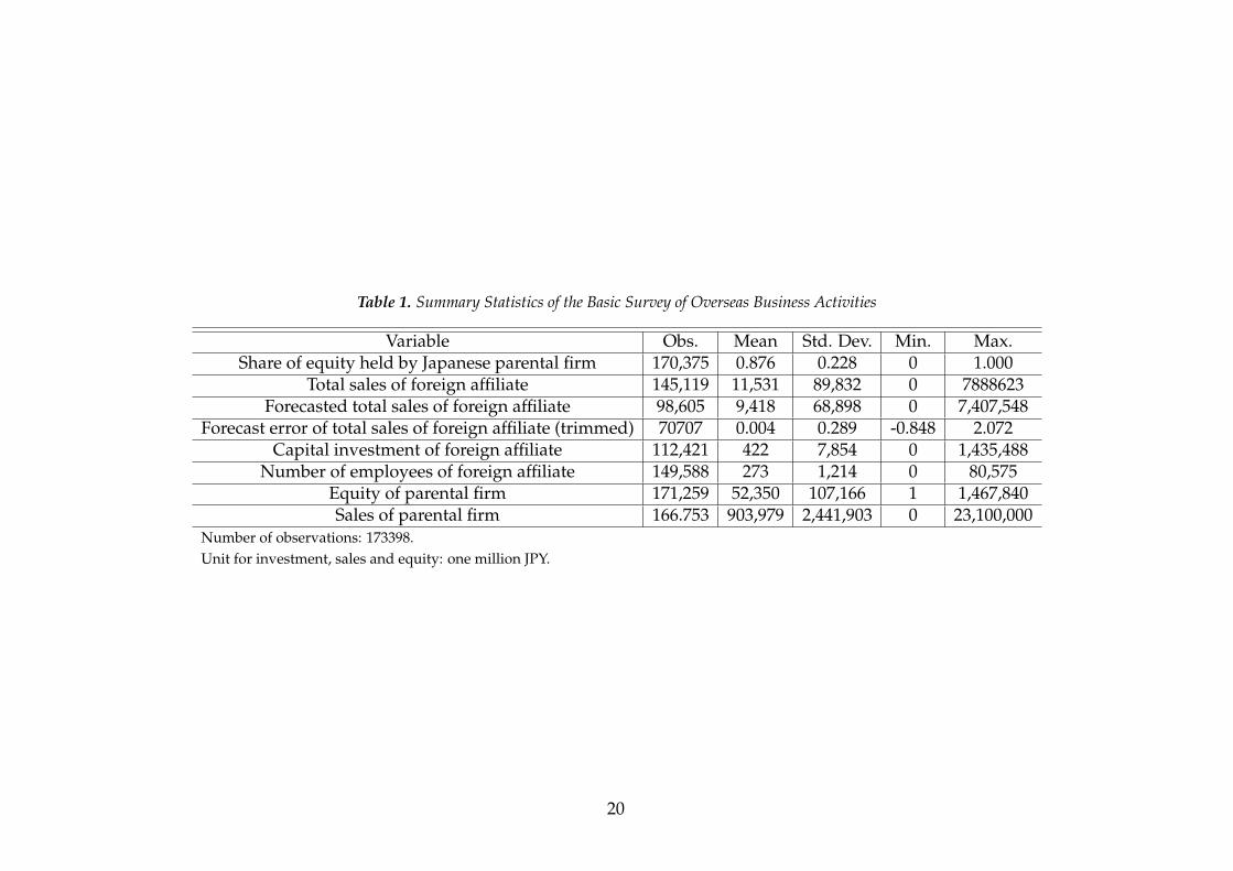
Table 1. Summary Statistics of the Basic Survey of Overseas Business Activities

Variable Obs. Mean Std. Dev. Min. Max.Share of equity held by Japanese parental firm 170,375 0.876 0.228 0 1.000

Total sales of foreign affiliate 145,119 11,531 89,832 0 7888623Forecasted total sales of foreign affiliate 98,605 9,418 68,898 0 7,407,548

Forecast error of total sales of foreign affiliate (trimmed) 70707 0.004 0.289 -0.848 2.072Capital investment of foreign affiliate 112,421 422 7,854 0 1,435,488

Number of employees of foreign affiliate 149,588 273 1,214 0 80,575Equity of parental firm 171,259 52,350 107,166 1 1,467,840Sales of parental firm 166.753 903,979 2,441,903 0 23,100,000

Number of observations: 173398.Unit for investment, sales and equity: one million JPY.

20

Table 2. Pre-trends for total sales

(1) (2) (3) (4) (5) (6) (7) (8)log(sales)sub log(sales)sub log(sales)sub log(sales)sub log(sales)sub log(sales)sub log(sales)sub log(sales)sub

Iyear≥2009*China 0.041 0.013[0.031] [0.023]

Iyear≥2010*China 0.074∗∗∗ 0.037∗

[0.024] [0.020]

Iyear≥2011*China -0.007 -0.031∗∗

[0.016] [0.014]

Iyear≥2012*China -0.062∗∗∗ -0.048∗∗∗

[0.019] [0.013]

log(emp)sub 0.441∗∗∗ 0.441∗∗∗ 0.441∗∗∗ 0.441∗∗∗

[0.063] [0.063] [0.063] [0.063]N 129742 129742 129742 129742 122720 122720 122720 122720adj. R2 0.931 0.931 0.931 0.931 0.943 0.943 0.943 0.943Standard errors are in parentheses.Standard errors are clustered at the country level.∗ p < 0.10, ∗∗ p < 0.05, ∗∗∗ p < 0.01Parent-level Controls: log(sales) and log(equity).Affiliate-level Control: log(sales).Country-level controls: log(GDP), log(GDP per capita), annual GDP growth rate.China and non-China specific linear time trends are included.Time span: 2007-2014.

21

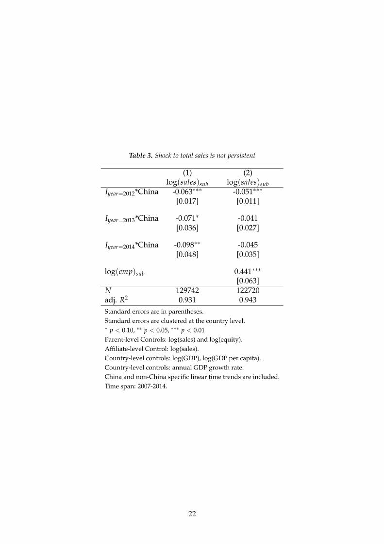
Table 3. Shock to total sales is not persistent

(1) (2)log(sales)sub log(sales)sub

Iyear=2012*China -0.063∗∗∗ -0.051∗∗∗

[0.017] [0.011]

Iyear=2013*China -0.071∗ -0.041[0.036] [0.027]

Iyear=2014*China -0.098∗∗ -0.045[0.048] [0.035]

log(emp)sub 0.441∗∗∗

[0.063]N 129742 122720adj. R2 0.931 0.943Standard errors are in parentheses.Standard errors are clustered at the country level.∗ p < 0.10, ∗∗ p < 0.05, ∗∗∗ p < 0.01Parent-level Controls: log(sales) and log(equity).Affiliate-level Control: log(sales).Country-level controls: log(GDP), log(GDP per capita).Country-level controls: annual GDP growth rate.China and non-China specific linear time trends are included.Time span: 2007-2014.

22

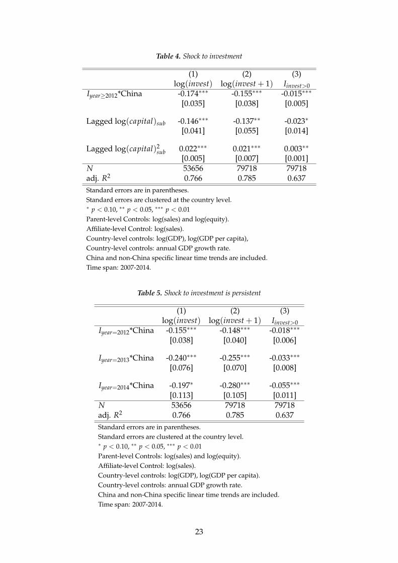
Table 4. Shock to investment

(1) (2) (3)log(invest) log(invest + 1) Iinvest>0

Iyear≥2012*China -0.174∗∗∗ -0.155∗∗∗ -0.015∗∗∗

[0.035] [0.038] [0.005]

Lagged log(capital)sub -0.146∗∗∗ -0.137∗∗ -0.023∗

[0.041] [0.055] [0.014]

Lagged log(capital)2sub 0.022∗∗∗ 0.021∗∗∗ 0.003∗∗

[0.005] [0.007] [0.001]N 53656 79718 79718adj. R2 0.766 0.785 0.637Standard errors are in parentheses.Standard errors are clustered at the country level.∗ p < 0.10, ∗∗ p < 0.05, ∗∗∗ p < 0.01Parent-level Controls: log(sales) and log(equity).Affiliate-level Control: log(sales).Country-level controls: log(GDP), log(GDP per capita),Country-level controls: annual GDP growth rate.China and non-China specific linear time trends are included.Time span: 2007-2014.

Table 5. Shock to investment is persistent

(1) (2) (3)log(invest) log(invest + 1) Iinvest>0

Iyear=2012*China -0.155∗∗∗ -0.148∗∗∗ -0.018∗∗∗

[0.038] [0.040] [0.006]

Iyear=2013*China -0.240∗∗∗ -0.255∗∗∗ -0.033∗∗∗

[0.076] [0.070] [0.008]

Iyear=2014*China -0.197∗ -0.280∗∗∗ -0.055∗∗∗

[0.113] [0.105] [0.011]N 53656 79718 79718adj. R2 0.766 0.785 0.637Standard errors are in parentheses.Standard errors are clustered at the country level.∗ p < 0.10, ∗∗ p < 0.05, ∗∗∗ p < 0.01Parent-level Controls: log(sales) and log(equity).Affiliate-level Control: log(sales).Country-level controls: log(GDP), log(GDP per capita).Country-level controls: annual GDP growth rate.China and non-China specific linear time trends are included.Time span: 2007-2014.

23

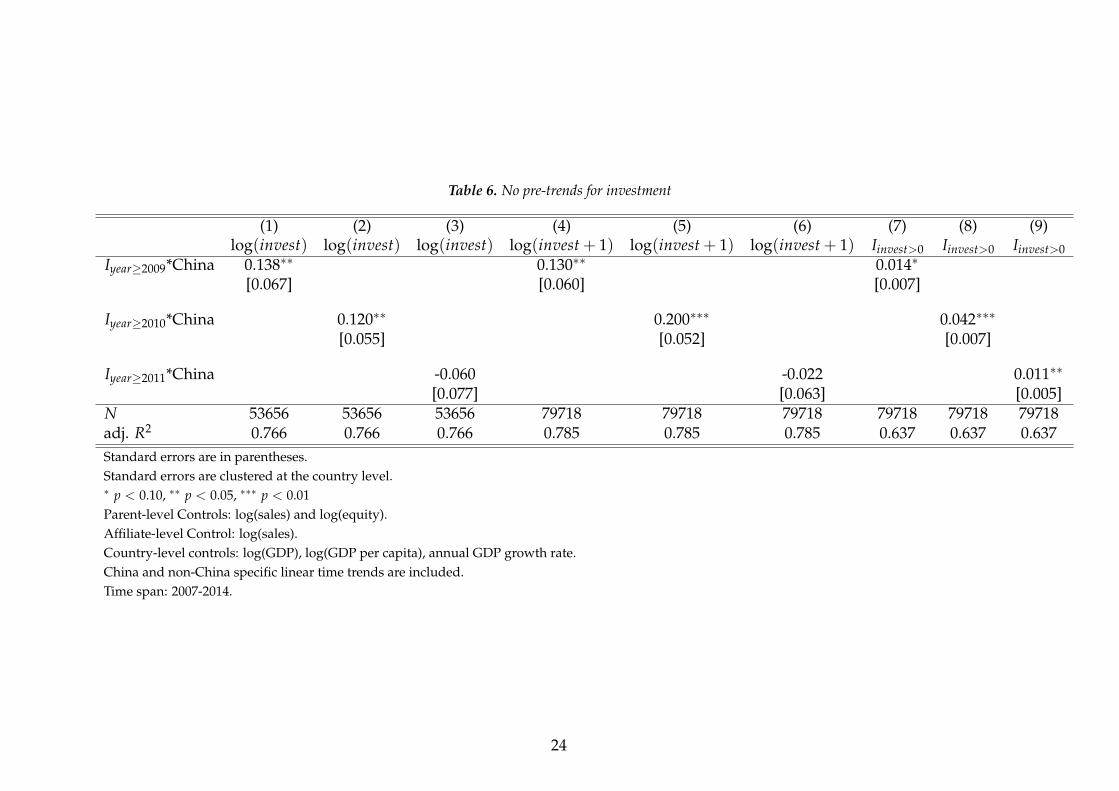
Table 6. No pre-trends for investment

(1) (2) (3) (4) (5) (6) (7) (8) (9)log(invest) log(invest) log(invest) log(invest + 1) log(invest + 1) log(invest + 1) Iinvest>0 Iinvest>0 Iinvest>0

Iyear≥2009*China 0.138∗∗ 0.130∗∗ 0.014∗

[0.067] [0.060] [0.007]

Iyear≥2010*China 0.120∗∗ 0.200∗∗∗ 0.042∗∗∗

[0.055] [0.052] [0.007]

Iyear≥2011*China -0.060 -0.022 0.011∗∗

[0.077] [0.063] [0.005]N 53656 53656 53656 79718 79718 79718 79718 79718 79718adj. R2 0.766 0.766 0.766 0.785 0.785 0.785 0.637 0.637 0.637Standard errors are in parentheses.Standard errors are clustered at the country level.∗ p < 0.10, ∗∗ p < 0.05, ∗∗∗ p < 0.01Parent-level Controls: log(sales) and log(equity).Affiliate-level Control: log(sales).Country-level controls: log(GDP), log(GDP per capita), annual GDP growth rate.China and non-China specific linear time trends are included.Time span: 2007-2014.

24

Table 7. Drop in investment: Investment Ratio

(1) (2) (3) (4)invest ratio invest ratio invest ratio invest ratio

Iyear≥2012*China -0.035∗∗ -0.032∗∗

[0.015] [0.015]

Iyear=2012*China -0.033∗∗ -0.028∗

[0.017] [0.016]

Iyear=2013*China -0.054∗∗∗ -0.035∗∗∗

[0.013] [0.012]

Iyear=2014*China -0.057∗∗∗ -0.024[0.019] [0.017]

Lagged LiquidityCapital 0.008∗∗∗ 0.008∗∗∗

[0.001] [0.001]N 78901 70197 78901 70197adj. R2 0.294 0.302 0.294 0.302Standard errors are in parentheses.Standard errors are clustered at the country level.Top and bottom one percent observations of investment ratio are trimmed.Top and bottom one percent observations of the liquidity-capital ratio are trimmed.∗ p < 0.10, ∗∗ p < 0.05, ∗∗∗ p < 0.01Parent-level Controls: log(sales) and log(equity).Country-level controls: log(GDP), log(GDP per capita), annual GDP growth rate.China and non-China specific linear time trends are included.Time span: 2007-2014.

25

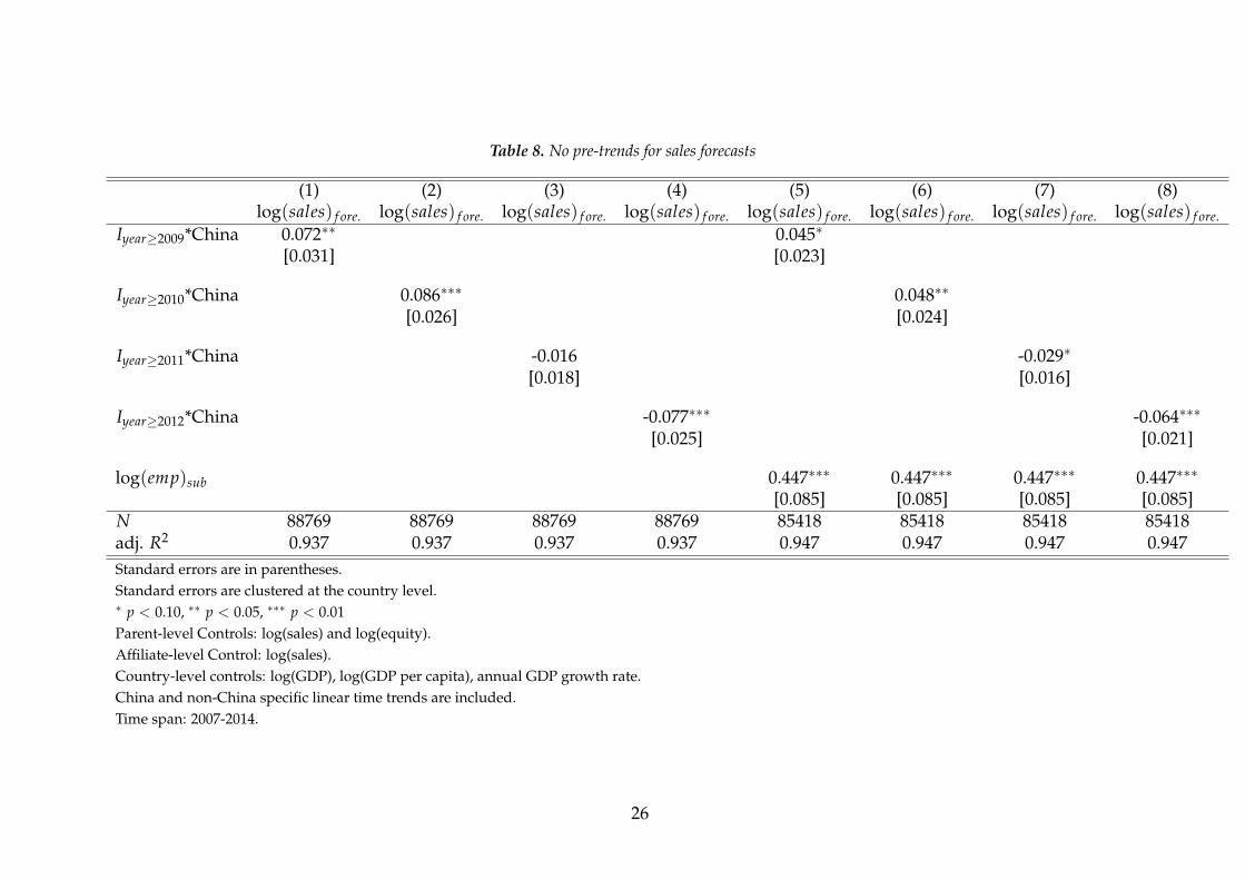
Table 8. No pre-trends for sales forecasts

(1) (2) (3) (4) (5) (6) (7) (8)log(sales) f ore. log(sales) f ore. log(sales) f ore. log(sales) f ore. log(sales) f ore. log(sales) f ore. log(sales) f ore. log(sales) f ore.

Iyear≥2009*China 0.072∗∗ 0.045∗

[0.031] [0.023]

Iyear≥2010*China 0.086∗∗∗ 0.048∗∗

[0.026] [0.024]

Iyear≥2011*China -0.016 -0.029∗

[0.018] [0.016]

Iyear≥2012*China -0.077∗∗∗ -0.064∗∗∗

[0.025] [0.021]

log(emp)sub 0.447∗∗∗ 0.447∗∗∗ 0.447∗∗∗ 0.447∗∗∗

[0.085] [0.085] [0.085] [0.085]N 88769 88769 88769 88769 85418 85418 85418 85418adj. R2 0.937 0.937 0.937 0.937 0.947 0.947 0.947 0.947Standard errors are in parentheses.Standard errors are clustered at the country level.∗ p < 0.10, ∗∗ p < 0.05, ∗∗∗ p < 0.01Parent-level Controls: log(sales) and log(equity).Affiliate-level Control: log(sales).Country-level controls: log(GDP), log(GDP per capita), annual GDP growth rate.China and non-China specific linear time trends are included.Time span: 2007-2014.

26

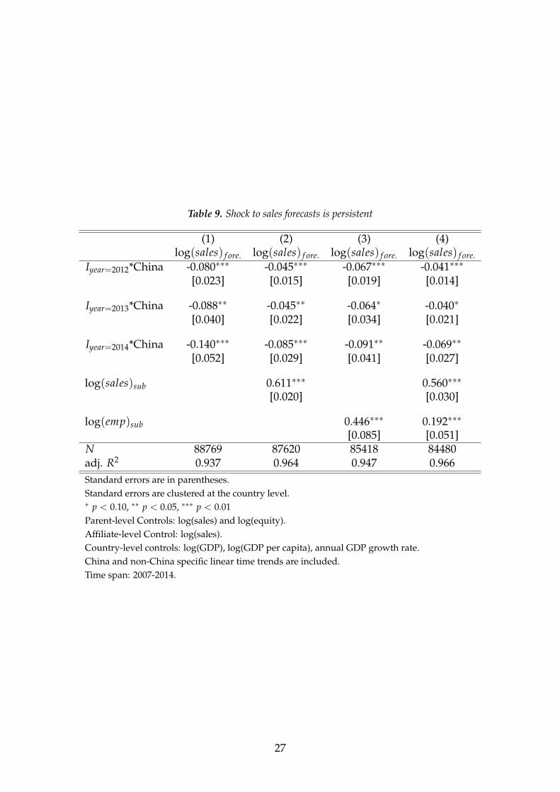
Table 9. Shock to sales forecasts is persistent

(1) (2) (3) (4)log(sales) f ore. log(sales) f ore. log(sales) f ore. log(sales) f ore.

Iyear=2012*China -0.080∗∗∗ -0.045∗∗∗ -0.067∗∗∗ -0.041∗∗∗

[0.023] [0.015] [0.019] [0.014]

Iyear=2013*China -0.088∗∗ -0.045∗∗ -0.064∗ -0.040∗

[0.040] [0.022] [0.034] [0.021]

Iyear=2014*China -0.140∗∗∗ -0.085∗∗∗ -0.091∗∗ -0.069∗∗

[0.052] [0.029] [0.041] [0.027]

log(sales)sub 0.611∗∗∗ 0.560∗∗∗

[0.020] [0.030]

log(emp)sub 0.446∗∗∗ 0.192∗∗∗

[0.085] [0.051]N 88769 87620 85418 84480adj. R2 0.937 0.964 0.947 0.966Standard errors are in parentheses.Standard errors are clustered at the country level.∗ p < 0.10, ∗∗ p < 0.05, ∗∗∗ p < 0.01Parent-level Controls: log(sales) and log(equity).Affiliate-level Control: log(sales).Country-level controls: log(GDP), log(GDP per capita), annual GDP growth rate.China and non-China specific linear time trends are included.Time span: 2007-2014.

27

Table 10. Shock to forecast errors

(1) (2)FEsales FEsales

Iyear≥2013*China 0.048∗∗∗ 0.052∗∗∗

[0.011] [0.011]

log(emp)sub 0.017∗∗

[0.008]N 66776 64276adj. R2 0.232 0.235Standard errors are in parentheses.Standard errors are clustered at the country level.∗ p < 0.10, ∗∗ p < 0.05, ∗∗∗ p < 0.01Top and bottom one percent observations of FEs are trimmed.Parent-level Controls: log(sales) and log(equity).Affiliate-level Control: log(sales).Country-level controls: log(GDP), log(GDP per capita).Country-level controls: annual GDP growth rate.China and non-China specific linear time trends are included.Time span: 2007-2014.

Table 11. Shock to forecast errors is persistent

(1) (2) (3) (4)FEsales FEsales FEsales FEsales

Iyear=2013*China 0.049∗∗∗ 0.057∗∗∗ 0.052∗∗∗ 0.057∗∗∗

[0.012] [0.009] [0.012] [0.010]

Iyear=2014*China 0.044∗∗∗ 0.052∗∗∗ 0.052∗∗∗ 0.055∗∗∗

[0.011] [0.009] [0.010] [0.009]

log(sales)sub 0.178∗∗∗ 0.205∗∗∗

[0.009] [0.011]

log(emp)sub 0.017∗∗ -0.057∗∗∗

[0.008] [0.012]N 66776 66776 64276 64276adj. R2 0.232 0.291 0.235 0.300Standard errors are in parentheses.Standard errors are clustered at the country level.Top and bottom one percent observations of forecast errors are trimmed.∗ p < 0.10, ∗∗ p < 0.05, ∗∗∗ p < 0.01Parent-level Controls: log(sales) and log(equity).Affiliate-level Control: log(sales).Country-level controls: log(GDP), log(GDP per capita).Country-level controls: annual GDP growth rate.China and non-China specific linear time trends are included.Time span: 2007-2014.

28

Table 12. No pre-trends for forecast errors

(1) (2) (3) (4) (5) (6) (7) (8)FEsales FEsales FEsales FEsales FEsales FEsales FEsales FEsales

Iyear≥2009*China -0.041∗∗ -0.046∗∗∗

[0.018] [0.017]

Iyear≥2010*China -0.009 -0.016[0.016] [0.016]

Iyear≥2011*China 0.016 0.015[0.012] [0.013]

Iyear≥2012*China -0.026∗ -0.025∗

[0.015] [0.015]

log(emp)sub 0.017∗∗ 0.017∗∗ 0.016∗∗ 0.016∗∗

[0.008] [0.008] [0.008] [0.008]N 66776 66776 66776 66776 64276 64276 64276 64276adj. R2 0.232 0.232 0.232 0.232 0.235 0.234 0.234 0.234Standard errors are in parentheses.Standard errors are clustered at the country level.Top and bottom one percent obs. of forecast errors are trimmed.∗ p < 0.10, ∗∗ p < 0.05, ∗∗∗ p < 0.01Parent-level Controls: log(sales) and log(equity).Affiliate-level Control: log(sales).Country-level controls: log(GDP), log(GDP per capita), annual GDP growth rate.China and non-China specific linear time trends are included.Time span: 2007-2014.

29

Table 13. Quantification: 2007-2012

(1) (2) (3) (4)log(invest) log(sales)sub log(sales) f ore. FEsales

Iyear≥2012*China -0.137∗∗∗ -0.083∗∗∗

[0.048] [0.021]

Iyear≥2013*China -0.020 0.054∗∗∗

[0.018] [0.012]Lagged log(capital)sub Included? Yes No No No

Lagged log(capital)2sub Included? Yes No No No

Lagged(

LiquidityCapital

)sub

Included? Yes No No No

Time span 2007-2012 2008-2013 2007-2012 2008-2013N 32648 97225 64088 56025adj. R2 0.773 0.940 0.944 0.233Standard errors are in parentheses.Standard errors are clustered at the country level.Top and bottom one percent observations of FEs are trimmed.Top and bottom one percent observations of the liquidity-capital ratio are trimmed.∗ p < 0.10, ∗∗ p < 0.05, ∗∗∗ p < 0.01Parent-level Controls: log(sales) and log(equity).Country-level controls: log(GDP), log(GDP per capita), and annual GDP growth rate.China and non-China specific linear time trends are included.

30

Table 14. Quantification: 2007-2012

(1) (2) (3) (4)log(invest) log(sales)sub log(sales) f ore. FEsales

Iyear≥2012*China -0.137∗∗∗ -0.092∗∗∗

[0.048] [0.020]

Iyear≥2013*China -0.018 0.060∗∗∗

[0.021] [0.013]Lagged log(capital)sub Included? Yes Yes Yes Yes

Lagged log(capital)2sub Included? Yes Yes Yes Yes

Lagged(

LiquidityCapital

)sub

Included? Yes Yes Yes Yes

Time span 2007-2012 2008-2013 2007-2012 2008-2013N 32648 68609 40523 50378adj. R2 0.773 0.946 0.954 0.234Standard errors are in parentheses.Standard errors are clustered at the country level.Top and bottom one percent observations of FEs are trimmed.Top and bottom one percent observations of the liquidity-capital ratio are trimmed.∗ p < 0.10, ∗∗ p < 0.05, ∗∗∗ p < 0.01Parent-level Controls: log(sales) and log(equity).Country-level controls: log(GDP), log(GDP per capita), and annual GDP growth rate.China and non-China specific linear time trends are included.

31

Table 15. Quantification: 2007-2013

(1) (2) (3) (4)log(invest) log(sales)sub log(sales) f ore. FEsales

Iyear≥2012*China -0.158∗∗∗ -0.082∗∗∗

[0.049] [0.026]

Iyear≥2013*China -0.025 0.048∗∗∗

[0.023] [0.011]Lagged log(capital)sub Included? Yes No No No

Lagged log(capital)2sub Included? Yes No No No

Lagged(

LiquidityCapital

)sub

Included? Yes No No No

Time span 2007-2013 2008-2014 2007-2013 2008-2014N 40108 115802 76370 66776adj. R2 0.768 0.936 0.941 0.232Standard errors are in parentheses.Standard errors are clustered at the country level.Top and bottom one percent observations of FEs are trimmed.Top and bottom one percent observations of the liquidity-capital ratio are trimmed.∗ p < 0.10, ∗∗ p < 0.05, ∗∗∗ p < 0.01Affiliate-level capital stock and liquidity ratio in 2012 are replaced by their values in 2011.Parent-level Controls: log(sales) and log(equity).Country-level controls: log(GDP), log(GDP per capita), and annual GDP growth rate.China and non-China specific linear time trends are included.

32

Table 16. Quantification: 2007-2013

(1) (2) (3) (4)log(invest) log(sales)sub log(sales) f ore. FEsales

Iyear≥2012*China -0.158∗∗∗ -0.088∗∗∗

[0.049] [0.023]

Iyear≥2013*China -0.024 0.052∗∗∗

[0.024] [0.011]Lagged log(capital)sub Included? Yes Yes Yes Yes

Lagged log(capital)2sub Included? Yes Yes Yes Yes

Lagged(

LiquidityCapital

)sub

Included? Yes Yes Yes Yes

Time span 2007-2013 2008-2014 2007-2013 2008-2014N 40108 80554 49654 58637adj. R2 0.768 0.943 0.950 0.224Standard errors are in parentheses.Standard errors are clustered at the country level.Top and bottom one percent observations of FEs are trimmed.Top and bottom one percent observations of the liquidity-capital ratio are trimmed.∗ p < 0.10, ∗∗ p < 0.05, ∗∗∗ p < 0.01Affiliate-level capital stock and liquidity ratio in 2012 are replaced by their values in 2011.Parent-level Controls: log(sales) and log(equity).Country-level controls: log(GDP), log(GDP per capita), and annual GDP growth rate.China and non-China specific linear time trends are included.

33

Figure 1. Share of Japanese FDI in China’s Total Inward FDI

0

.1

.2

2009q1 2010q3 2012q1 2013q3 2015q1

Total FDI Manufacturing FDINonmanufacturing FDI

Note: The vertical line indicates 2012/Q3, the quarter in which the Island Crisis happened. Japanese quarterlyFDI data are obtained from the Bank of Japan. Quarterly total FDI inflows into China are obtained from ChinaData Online. We partition the quarterly total FDI inflows into manufacturing and non-manufacturing FDIusing their ratios in the yearly total FDI inflows.

34

Figure 2. Histogram of Forecast Errors for Total Sales

0.5

11.

52

2.5

Den

sity

-1 0 1 2Sales Forecast Errors

Note: Histogram of FEt with fitted normal density. FEt is the forecast error of sales, defined asSalest/Et−1(Salest)− 1.

Figure 3. Employment Distribution of Reporting and Non-reporting Observations: All Affiliates

0.0

5.1

.15

.2D

ensi

ty

0 5 10log(Empolyment)

Forecast reporter Forecast non-reporter

Distribution of Log Employment of Reporting and Non-reporting Observations

35

Figure 4. Sales Distribution of Reporting and Non-reporting Observations: All Affiliates

0.0

5.1

.15

.2D

ensi

ty

0 5 10 15log(Sales)

Forecast reporter Forecast non-reporter

Distribution of Log Sales of Reporting and Non-reporting Observations

Figure 5. Employment Distribution of Reporting and Non-reporting Observations: Affiliates in China

0.0

5.1

.15

.2.2

5D

ensi

ty

0 5 10log(Empolyment), China

Forecast reporter Forecast non-reporter

Distribution of Log Employment of Reporting and Non-reporting Observations

36

Figure 6. Sales Distribution of Reporting and Non-reporting Observations: Affiliates in China

0.0

5.1

.15

.2.2

5D

ensi

ty

0 5 10 15log(Sales), China

Forecast reporter Forecast non-reporter

Distribution of Log Sales of Reporting and Non-reporting Observations

Figure 7. Distribution of Annual Growth Rate of Total Sales

0.5

11.

52

Den

sity

-1 -.5 0 .5 1Annual growth rate of total sales

2011 20122013 2014

Plotted from our unbalanced panel using the firm-level data of the Basic Survey of Overseas BusinessActivities released by the Ministry of Economy, Trade and Industry. Observations with growth rateequals −100% or higher than 100% are excluded.

37

Figure 8. Trend of Average Sales of Japanese Affiliates

6.6

6.8

77.

27.

47.

6Av

erag

e Sa

les

2006 2008 2010 2012 2014year

Non-China China

Figure 9. Trend of Average Log Investment of Japanese Affiliates

3.4

3.6

3.8

44.

2Av

erag

e lo

g in

vest

men

t

2006 2008 2010 2012 2014year

Non-China China

38

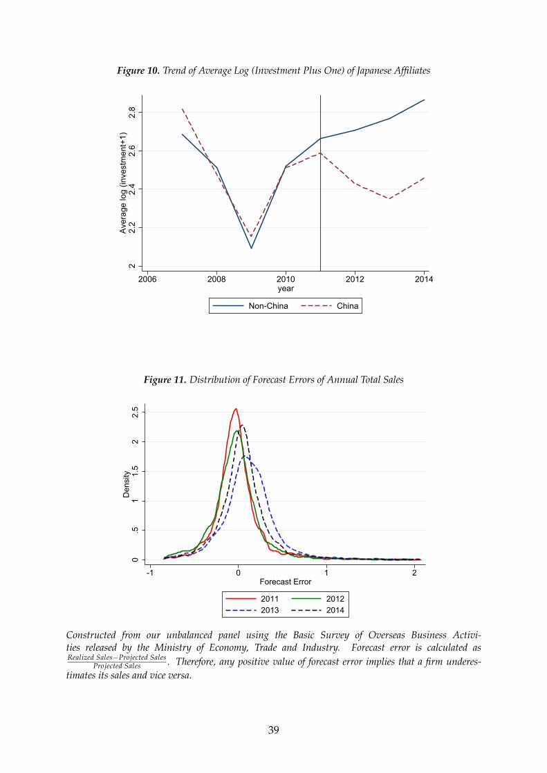
Figure 10. Trend of Average Log (Investment Plus One) of Japanese Affiliates

22.

22.

42.

62.

8Av

erag

e lo

g (in

vest

men

t+1)

2006 2008 2010 2012 2014year

Non-China China

Figure 11. Distribution of Forecast Errors of Annual Total Sales

0.5

11.

52

2.5

Den

sity

-1 0 1 2Forecast Error

2011 20122013 2014

Constructed from our unbalanced panel using the Basic Survey of Overseas Business Activi-ties released by the Ministry of Economy, Trade and Industry. Forecast error is calculated asRealized Sales−Projected Sales

Projected Sales . Therefore, any positive value of forecast error implies that a firm underes-timates its sales and vice versa.

39

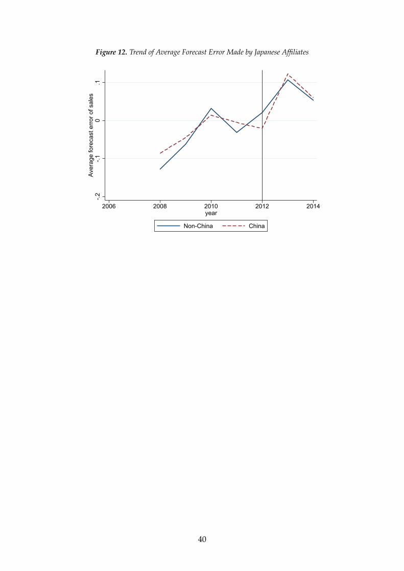
Figure 12. Trend of Average Forecast Error Made by Japanese Affiliates

-.2-.1

0.1

Aver

age

fore

cast

erro

r of s

ales

2006 2008 2010 2012 2014year

Non-China China

40

Online Appendix: Not for Publication

Table 17. Drop in total sales (2009 excluded)

(1) (2) (3) (4)log(sales)sub log(sales)sub log(sales)sub log(sales)sub

Iyear≥2012*China -0.062∗∗∗ -0.046∗∗∗

[0.017] [0.012]

Iyear=2012*China -0.063∗∗∗ -0.049∗∗∗

[0.014] [0.010]

Iyear=2013*China -0.072∗∗ -0.035[0.034] [0.026]

Iyear=2014*China -0.096∗∗ -0.036[0.045] [0.034]

log(emp)sub 0.448∗∗∗ 0.448∗∗∗

[0.064] [0.064]N 114586 114586 108331 108331adj. R2 0.930 0.930 0.942 0.942Standard errors are in parentheses.Standard errors are clustered at the country level.∗ p < 0.10, ∗∗ p < 0.05, ∗∗∗ p < 0.01Parent-level Controls: log(sales) and log(equity).Country-level controls: log(GDP), log(GDP per capita), and annual GDP growth rate.China and non-China specific linear time trends are included.Time span: 2007-2008 and 2010-2014.

41

Table 18. Drop in investment (2009 excluded)

(1) (2) (3) (4) (5) (6)log(invest) log(invest) log(invest + 1) log(invest + 1) Iinvest>0 Iinvest>0

Iyear≥2012*China -0.158∗∗∗ -0.143∗∗∗ -0.014∗∗

[0.035] [0.037] [0.006]

Iyear=2012*China -0.140∗∗∗ -0.137∗∗∗ -0.017∗∗∗

[0.038] [0.039] [0.006]

Iyear=2013*China -0.227∗∗∗ -0.246∗∗∗ -0.029∗∗∗

[0.078] [0.071] [0.008]

Iyear=2014*China -0.192∗ -0.272∗∗∗ -0.049∗∗∗

[0.112] [0.102] [0.011]

Lagged log(capital)sub -0.211∗∗∗ -0.211∗∗∗ -0.218∗∗∗ -0.218∗∗∗ -0.020∗ -0.020∗

[0.048] [0.048] [0.060] [0.060] [0.011] [0.011]

Lagged log(capital)2sub 0.028∗∗∗ 0.028∗∗∗ 0.029∗∗∗ 0.029∗∗∗ 0.002∗∗ 0.002∗∗

[0.005] [0.005] [0.007] [0.007] [0.001] [0.001]N 46836 46836 68241 68241 68241 68241adj. R2 0.774 0.774 0.790 0.790 0.642 0.642Standard errors are in parentheses.Standard errors are clustered at the country level.∗ p < 0.10, ∗∗ p < 0.05, ∗∗∗ p < 0.01Parent-level Controls: log(sales) and log(equity).Country-level controls: log(GDP), log(GDP per capita), and annual GDP growth rate.China and non-China specific linear time trends are included.Time span: 2007-2008 and 2010-2014.

42

Table 19. Drop in projected sales (2009 excluded)

(1) (2) (3) (4) (5) (6)log(sales) f ore. log(sales) f ore. log(sales) f ore. log(sales) f ore. log(sales) f ore. log(sales) f ore.

Iyear≥2012*China -0.074∗∗∗ -0.060∗∗∗

[0.024] [0.021]

Iyear=2012*China -0.078∗∗∗ -0.043∗∗∗ -0.064∗∗∗ -0.039∗∗∗

[0.022] [0.015] [0.019] [0.014]

Iyear=2013*China -0.085∗∗ -0.045∗∗ -0.058∗ -0.040∗

[0.040] [0.022] [0.034] [0.022]

Iyear=2014*China -0.135∗∗∗ -0.083∗∗∗ -0.084∗∗ -0.069∗∗

[0.050] [0.029] [0.041] [0.027]

log(sales)sub 0.624∗∗∗ 0.571∗∗∗

[0.022] [0.034]

log(emp)sub 0.454∗∗∗ 0.453∗∗∗ 0.189∗∗∗

[0.088] [0.088] [0.054]N 78616 78616 77545 75620 75620 74734adj. R2 0.936 0.936 0.964 0.946 0.946 0.966Standard errors are in parentheses.Standard errors are clustered at the country level.∗ p < 0.10, ∗∗ p < 0.05, ∗∗∗ p < 0.01Parent-level Controls: log(sales) and log(equity).Country-level controls: log(GDP), log(GDP per capita), and annual GDP growth rate.China and non-China specific linear time trends are included.Time span: 2007-2008 and 2010-2014.

43

Table 20. Change in forecast errors (2009 excluded)

(1) (2) (3) (4) (5) (6)FEsales FEsales FEsales FEsales FEsales FEsales

Iyear≥2013*China 0.052∗∗∗ 0.056∗∗∗

[0.011] [0.010]

Iyear=2013*China 0.052∗∗∗ 0.060∗∗∗ 0.056∗∗∗ 0.059∗∗∗

[0.012] [0.009] [0.011] [0.010]

Iyear=2014*China 0.051∗∗∗ 0.059∗∗∗ 0.059∗∗∗ 0.061∗∗∗

[0.010] [0.008] [0.009] [0.008]

log(sales)sub 0.178∗∗∗ 0.208∗∗∗

[0.009] [0.011]

log(emp)sub 0.015∗ 0.015∗ -0.060∗∗∗

[0.008] [0.008] [0.013]N 57937 57937 57937 55740 55740 55740adj. R2 0.248 0.248 0.306 0.251 0.251 0.316Standard errors are in parentheses.Standard errors are clustered at the country level.∗ p < 0.10, ∗∗ p < 0.05, ∗∗∗ p < 0.01Top and bottom one percent observations of FEs are trimmed.Parent-level Controls: log(sales) and log(equity).Country-level controls: log(GDP), log(GDP per capita), and annual GDP growth rate.China and non-China specific linear time trends are included.Time span: 2007-2008 and 2010-2014.

44

Table 21. Drop in total sales (starting from 2010)

(1) (2) (3) (4)log(sales)sub log(sales)sub log(sales)sub log(sales)sub

Iyear≥2012*China -0.031∗∗ -0.042∗∗∗

[0.014] [0.013]

Iyear=2012*China -0.040∗∗∗ -0.018[0.015] [0.014]

Iyear=2013*China -0.039 0.012[0.029] [0.025]

Iyear=2014*China -0.053 0.031[0.049] [0.037]

log(emp)sub 0.381∗∗∗ 0.381∗∗∗

[0.058] [0.058]N 85788 85788 81016 81016adj. R2 0.948 0.948 0.956 0.956Standard errors are in parentheses.Standard errors are clustered at the country level.∗ p < 0.10, ∗∗ p < 0.05, ∗∗∗ p < 0.01Parent-level Controls: log(sales) and log(equity).Country-level controls: log(GDP), log(GDP per capita), and annual GDP growth rate.China and non-China specific linear time trends are included.Time span: 2010-2014.

45

Table 22. Drop in investment (starting from 2010)

(1) (2) (3) (4)log(invest) log(invest) log(invest + 1) log(invest + 1)

Iyear≥2012*China -0.095∗∗ -0.045[0.047] [0.044]

Iyear=2012*China -0.046 -0.014[0.058] [0.049]

Iyear=2013*China -0.083 -0.035[0.140] [0.102]

Iyear=2014*China 0.007 0.020[0.212] [0.158]

Lagged log(capital)sub -0.252∗∗∗ -0.251∗∗∗ -0.223∗∗∗ -0.223∗∗∗

[0.053] [0.052] [0.074] [0.074]

Lagged log(capital)2sub 0.023∗∗∗ 0.022∗∗∗ 0.018∗∗ 0.018∗∗

[0.006] [0.006] [0.007] [0.007]N 39885 39885 57429 57429adj. R2 0.789 0.789 0.809 0.809Standard errors are in parentheses.Standard errors are clustered at the country level.∗ p < 0.10, ∗∗ p < 0.05, ∗∗∗ p < 0.01Parent-level Controls: log(sales) and log(equity).Country-level controls: log(GDP), log(GDP per capita), and annual GDP growth rate.China and non-China specific linear time trends are included.Time span: 2010-2014.

46

Table 23. Drop in projected sales (starting from 2010)

(1) (2) (3) (4) (5) (6)log(sales) f ore. log(sales) f ore. log(sales) f ore. log(sales) f ore. log(sales) f ore. log(sales) f ore.

Iyear≥2012*China -0.021∗ -0.031∗∗

[0.011] [0.012]

Iyear=2012*China -0.034∗ -0.018 -0.027 -0.010[0.018] [0.019] [0.018] [0.020]

Iyear=2013*China -0.022 -0.003 -0.002 0.011[0.034] [0.028] [0.034] [0.031]

Iyear=2014*China -0.048 -0.025 -0.009 0.003[0.047] [0.038] [0.042] [0.038]

log(sales)sub 0.534∗∗∗ 0.487∗∗∗

[0.027] [0.034]

log(emp)sub 0.417∗∗∗ 0.417∗∗∗ 0.207∗∗∗

[0.082] [0.082] [0.053]N 57620 57620 56746 55424 55424 54701adj. R2 0.952 0.952 0.969 0.958 0.958 0.971Standard errors are in parentheses.Standard errors are clustered at the country level.∗ p < 0.10, ∗∗ p < 0.05, ∗∗∗ p < 0.01Parent-level Controls: log(sales) and log(equity).Country-level controls: log(GDP), log(GDP per capita), and annual GDP growth rate.China and non-China specific linear time trends are included.Time span: 2010-2014.

47

Table 24. Change in forecast errors (starting from 2010)

(1) (2) (3) (4) (5) (6)FEsales FEsales FEsales FEsales FEsales FEsales

Iyear≥2013*China 0.057∗∗∗ 0.056∗∗∗

[0.015] [0.014]

Iyear=2013*China 0.058∗∗∗ 0.056∗∗∗ 0.057∗∗∗ 0.052∗∗∗

[0.015] [0.014] [0.014] [0.013]

Iyear=2014*China 0.063∗∗∗ 0.058∗∗ 0.066∗∗∗ 0.053∗∗

[0.021] [0.024] [0.022] [0.025]

log(sales)sub 0.209∗∗∗ 0.238∗∗∗

[0.013] [0.015]

log(emp)sub 0.012 0.012 -0.063∗∗∗

[0.008] [0.008] [0.013]N 48619 48619 48619 46767 46767 46767adj. R2 0.240 0.240 0.304 0.240 0.240 0.311Standard errors are in parentheses.Standard errors are clustered at the country level.∗ p < 0.10, ∗∗ p < 0.05, ∗∗∗ p < 0.01Top and bottom one percent observations of FEs are trimmed.Parent-level Controls: log(sales) and log(equity).Country-level controls: log(GDP), log(GDP per capita), and annual GDP growth rate.China and non-China specific linear time trends are included.Time span: 2010-2014.

48

This working paper has been produced bythe School of Economics and Finance atQueen Mary University of London

School of Economics and Finance Queen Mary University of LondonMile End RoadLondon E1 4NSTel: +44 (0)20 7882 7356Fax: +44 (0)20 8983 3580Web: www.econ.qmul.ac.uk/research/workingpapers/

Dpqzsjhiu ê 3128 Difoh Difo,Ubutvsp Tfohb, Diboh Tvo boeIpohzpoh [iboh bmm sjhiut sftfswfe

School of Economics and Finance