d. s. g. pollock department of economics queen …. s. g. pollock department of economics queen mary...

D. S. G. Pollock

Department of Economics Queen Mary College Mile End Road London, El 4NS, England

Submitted by Ingram Olkin

ABSTRACT

This paper sets forth some of the principal results of the algebra of Kronecker products in a way which relates them directly to the abstract algebra of tensor products. The concepts and the results that are developed in this way are used to analyse three alternative definitions that have been proposed for the derivative of a matrix function Y = Y(X) with respect to its matrix argument X. It is argued that only one of these definitions is viable. The other definitions, which are widely used in econometrics, are not consistent with the classical representation of linear algebra via matrix theory; and they lead to serious practical difficulties that do not arise when the appropriate definition is adopted.

INTRODUCTION

Over the last decade, there has been a growing interest amongst statisticians in the algebra of the Kronecker product of matrices and in the associated operation of matrix vectorization. Interest in this algebra has been motivated largely by the fact that it enables us to treat matrix equations as if

they were vector equations. Thus, by using the Kronecker product, we can write a matrix equation of the form Y = AXB’ as a vector equation of the

form Yc = (B @ A)X", where Y” and Xc are long vectors formed by a vertical arrangement of the columns of Y and X, and B @ A is the Kronecker product of B and A.

In multivariate statistical analysis, a straightforward use of this result is made, for example, in converting the equations of a multivariate regression model, which has many dependent variables, to a form which is isomorphic to the equation of a univariate regression model which has a single dependent

LINEAR ALGEBRA AND ITS APPLICATIONS 67:169-193 (1985) 169

( Elsevier Science Publishing Co., Inc., 1985 52 Vanderbilt Ave., New York, NY 10017 00243795/85/$3.30

170 D. S. G. POLLOCK

variable. This enables us to apply the statistical theory of the univariate model directly to the multivariate model.

The Kronecker product has had a long history, some of which Henderson and Searle have briefly recounted in [ll] and [12]. However, until recently, it had not been used sufficiently in any area of applied mathematics for a complete and readily accessible collection of results to have been amassed. Consequently, much of what is now available to statisticians has been invented or rediscovered by them. It is difficult, therefore, to know where to attribute the seminal ideas. Nevertheless, there is no doubt that the use of the Kronecker product by Zellner [28] in presenting his results on the estimation of seemingly unrelated regression equations strongly influenced the econometricians; and they have probably used the product more than any other group of statisticians.’ Neudecker subsequently set forth in [20], [21], and [22] a number of results concerning Kronecker products and matrix differential calculus that have proved important in practice, and Nissen [24], amongst others, must be given credit for underlining the logic of the process of vectorization.

Statisticians now have at their disposal a large body of results concerning the Kronecker product and its uses in matrix differential calculus, which has been systematically surveyed recently by several authors (see, for example, Balestra [2], Graham [9], Rogers [26], Nel [19], and the aforementioned Henderson and Searle [ll], [ 121). H owever, much of the theory retains an arcane and complicated aspect. It is our contention that much of this difficulty can be relieved by adopting a more formal approach to the algebra of Kronecker products, depending less upon the manipulation of matrices and more upon the abstract algebra of tensor products, to which statisticians have, so far, made virtually no reference.

The first purpose of this paper is therefore to set forth some of the principal results of the algebra of Kronecker products in a way that relates them directly to the algebra of tensor products. A seminal account of the abstract algebra of tensor products was provided by a group of French mathematicians writing in the early postwar years under the name of Bourbaki [4]. More recent and more extensive accounts of the algebra have been given by Marcus [18] and Greub [lo], as well as in subsequent editions of Bourbaki. We believe that many results that are the products of arduous matrix

‘However, we should not overlook the fact that marginal uses of the Kronecker product and the vectorization operator had heen made a decade earlier in the papers of the Cowles Commission for Research in Economics. See, for example, Chemoff and Divinsky [S] and Koopmans et al. [ 131; in both there are references to MacDuffee [15].

TENSOR PRODUCTS 171

manipulations can be seen as straightforward consequences of the rules of this algebra.

The other purpose of this paper is to use the concepts that are expounded in its early sections to analyse some of the alternative definitions that have been proposed for the derivative of a matrix function Y = Y(X) with respect to its matrix argument X. In particular, we shall consider three alternative definitions that are in common use, and we shall establish relationships amongst them. We shall argue that only one of these definitions is viable. The other definitions, which are widely used in econometrics, are not consistent with the classical representation of linear algebra via matrix theory, and they lead to serious practical difficulties that do not arise when the appropriate definition is adopted.

TENSOR PRODUCTS

In this section, we shall formalize some basic concepts and we shall supply some of the notation used hereafter. Throughout the paper, we shall attempt to avoid the use of the concept of an inner product defined on a Euclidean space by using, instead, the concept of a dual space of linear functionals. This should lead to a simpler account. However, since we shall work with real coordinate spaces and since we shall choose their natural bases, the full structure of Euclidean spaces will be at our disposal.

A summary of the notation that is used throughout the paper is provided in an appendix which might be profitably consulted on a number of occa- sions.

Basic Definitions Let us denote by V and ?V two real coordinate vector spaces of

dimension Dim+‘- = n and Dimw = m respectively, and let us denote the real line by 9’. The set of all linear transformations mapping from V to w denoted by 6p( y, %‘-) is itself a vector space of dimension Dim 2 = Dim Y xDirn#‘- = nm.

The dual space of 9’- is defined as the set V * = 2(V, 9%‘) of all linear transformations mapping from V onto the real line 9. Clearly, we have Dim V * = Dim V = n. We shall distinguish the elements of dual spaces by writing them with superscripts. The image of a vector x E V under the mapping u* E -Y-* will be denoted by

p = (o*, r), pE.9. 01


The dual space w * of -W is defined in the same manner. The natural basis of the primal space Y is the set of vectors ej,

j=l >**., n, that constitute the columns of the identity matrix I, of order n. The natural basis of the dual space V” * is the set of vectors e *j, j = 1,. . . , n, defined by the condition (e * j, ei) = ai j, i = 1,. . . , n, where aii is the Kronecker delta. In effect, e*j maps the basis vector ej E V into unity and all other basis vectors into zero. We can identify the elements of the natural basis V * with the rows of the identity matrix I,.

Weshalldenotethenaturalbasesof w and YY* bye,, i=l,...,m,and ,*i ) i=l ,***, m , respectively.

The vector w E w can be expressed in terms of the natural basis by writing

w = C (e*‘, w)e,. (2)

The scalars (e *i, w ) are the coordinates of the vector. Likewise, for w* E %‘- * we have the expression

w* = C<w*, ei)e*i, (3)

where (w*, ei) are the coordinates of w* relative to the dual basis of e *i, i=l ,..., m, of 7V*.

The transpose of w is the vector w’ E %‘- * whose coordinates relative to the dual basis are the same as the coordinates of w. Thus

w’= C(e*i, w>e*‘, (4)

where (e*‘, w) = (w’, ei). It is clear that, according to this definition, the transposes of the basis vectors ei, i = 1,. . . , m, of ?F are the basis vectors e *‘, i=l ,..., m, of 7V*.

Elementary Tensor Products

We can now proceed to define three types of elementary tensor products. In defining these products, we can use the notation that is normally associated with the Kronecker product of two matrices. We may therefore recall that if A = [ski] is an s X m matrix and if B = [bli] is an t X n matrix, then their

TENSOR PRODUCTS 173

Kronecker product (B@A) = [bljA] is an st x mn matrix whose ljth partition is brjA.

For the first definition, we consider the product ej Q e, which is an mn X 1 column vector with a unit in the [(j - 1)m + i]th position and zeros elsewhere. The tensor product V B V of the two primal spaces is defined as the set of all vectors of the form

Xc = Cxij(ej@ei).

ij

(5)

We describe the elements of the vector space V @ YY as contravariant tensor products. If xii = wivj for all i, j, then we can write

Xc= Cwivj(ejBei) ij

= CvjejE3 Cw,e,

i i

= v8w (6)

for some o E Y and w E ?Y. Elements that can be written in this form are said to be decomposable. Clearly, the set of all decomposable tensor products is of negligible extent in the context of the space as a whole. However, we can often simplify matters by considering decomposable products, and, since the operations that we shall be investigating are linear, we shall find that this entails no great loss of generality.

For the second definition, we consider the product e *i @e*j, which is a 1 x mn row vector with a unit in the [(i - l)n + j]th position and zeros elsewhere. The tensor product YY * @ -Y * of the two dual spaces is defined as the set of all vectors of the form

X'= Cxij(e*‘@e*j). ij

(7)

We describe the elements of the space %Y *@ V * as covariant tensor products.

The tensor product space ZV *BY* is not the same as the space Y * @ YY *. We can identify the latter with the dual space of V B w. Thus, if v, w, v*, and w* are elements of V, PV, V*, and YY* respectively, we


may define a linear functional on 7v @ w of the form

(v*@w*,v@w) = (o*, u)(w*,w). (8)

For the third definition, we consider the product e *j@ ei = e, 8 e * j, which is an m X n matrix with a unit in the ijth position and zeros elsewhere. Then the tensor product of the primal space YV and the dual space V * is defined as the set of all matrices of the form

X = Cxij(e*j@ei) ij

= &ij(eise*j). (9)

ij

We describe the elements of the space V*@#‘- as mixed tensor products. We should notice that, in this definition of mixed tensor products, the

positions of the dual and primal basis vectors are interchangeable. This does not imply that the operation of forming a mixed tensor product is a commuta- tive one; for, by identifying the elements in a decomposable mixed product as coming from a primal and a dual space respectively, we are essentially identifying their order in the product.

The tensor product space V *@ w may be identified with the set S?(V, w) of all linear transformations mapping from V to 7Y. Let u E V by any vector, and let u* E V * be regarded as an element of the set S?( V, 9). Then (o*, v) E 9%’ is a scalar and, on writing

(u*@w)u = (?I*, u)w, WEW", 00)

we identify the product u*@ w as an element of 9( V, l”y). Likewise, by writing w*(u*@w)= (w*, w)v*, we may also identify v*@w as an element of the set Z(YY *, V*) of adjoint transformations mapping from w * to V *. It is also clear from these examples that all decomposable elements of the space V * 8 w correspond to transformations of rank 1 and thus, since we are, in fact, dealing in terms of coordinate spaces, to matrices of rank 1. We might also note that, when DimV * = Dim YV, we have a square matrix for which the trace is defined by

Trace(u*@w) = (o*, w). (II)

TENSOR PRODUCTS 175

Multiple Tensor Products In general, the operation of forming tensor products may be regarded as a

noncommutative associative operation that can be applied to a succession of primal (or contravariant) and dual (or covariant) vectors. The noncommutativ- ity implies that the order amongst the covariant elements and the order amongst the contravariant elements must be preserved. However, the formal property of elementary mixed tensor products, manifested in (9) which allows the primal and the dual vectors to exchange their positions, implies that, in a multiple product, we are free to intersperse the covariant and the contravariant elements.

As an example, we may consider the Kronecker tensor product of the s x m matrix A = [ski] E W*@2 and the t X n matrix B = [blj] E Y*@9. These matrices may be expressed, in terms of the natural bases of the spaces, as mixed tensors. Thus

A = Caki(e,C3e**“), ki

B = Cblj(elBe*j).

li (12)

The Kronecker product of the two matrices can be expressed in any of the following ways:

g@A = xbljuki(e*i@e*i@el@ek)

= xbliuki(el@e*i@ek@e*i)

= Cbljaki(e*jgel~e*‘~ek)

= Cbljaki(elQekOe*j@e*‘), (13)

where it is understood that the summation is over all four indices. These alternative forms represent four out of a total of six possibilities.

EXAMPLE I. The expressions in (1 l), (12), and (13) facilitate the derivation of a familiar result concerning the trace of the Kronecker product of square matrices. Consider the definition

Trace(A)= xakj(e*iYe,). (14)


By extension, we have

Trace(B@A) = Cblja,,(e*j~e*‘,e,~e,)

= Cblj(e*‘, e,) Caki(e*i, e,>)

= Trace(B) Trace(A). (15)

Graham [9] quotes the usual derivation of this result.

Scalar Products A final point that needs to be noted in this section is the fact that, in

forming the tensor product of a vector space and the field of scalars 2, which may be considered as a vector space of dimension 1, we obtain just the vector space itself. Thus we have V-89 = V, %‘@V = Y, Y*@W = V*, and so forth. It follows that, if p E R, v E F, and v* E V*, then ~8.u = v@p = pv, p@v*= v*@p and, in particular, l@v=v@l=v.

Since the field of scalars is both a primal space and a dual space, it follows from the pseudocommutativity of mixed tensor products manifested in (9) and (13) that we may interpose a scalar X at any point in a multiple product. Thus we have A@(~@to)=(A@v)@w = v@(X@w) or, equivalently,

X(vc3Jw) = hv@w

= v8hw. (16)

We shall describe this property as the mobility of scalar multiplication.

COMPOSITIONS

We shall now define an operation of composition. Let V, -W be primal spaces, and let Y *, g* be dual spaces; and consider the elements v, w, v*, and g* taken from each of these spaces respectively. Then the composition of the mixed tensor products w@v* and v@g* is defined by writing

(w@v*)(v@g*)= (v*,v)(w@g*). (17)

An important specialization arises in the case where g* is the unit scalar. Then we have

(wev*)(vsl)=(w60v*)v

= co*> v)w. (18)

TENSOR PRODUCTS 177

This is exactly in accordance with the expression in (10) which identifies the mixed tensor product w@u* with an element in the set of linear transformations Y( V, W).

It may also be instructive to consider the composition of the three products A = q@ w*, X = w@v*, and D = v@g*. When this is written as

AXD= A(w@o*)D

= Aw@v*D

= ( w*, w)q@ (v*, ti>g*, (19)

it may be interpreted as the product of the image of w under the transformation A E Y(W, 2) with the image of v* under the adjoint transformation DE ~(~*,~**).

These operations of compositions extend, of course, to nondecomposable tensor products, as we shall see in a subsequent example. They also extend to multiple products. Consider the products A = q@ w*, B = p@ v*, C = w @ h*, and D = v@g*. Then we have

B@A = p@q@v*@w*,

D@c= v@w@g*@h*; (20)

and, from rules already stated, it follows that

(BBA)(DW) = (v*c~~*, vt3ww)(p~q~g**h*)

= co*, V>b@g*)@(w*, w)(q@h*)

= BD@Ac. (21)

This virtually establishes the associative law of multiplication for the Kronecker products of matrices. Complete generality is achieved when, instead of the decomposable tensor products that we have considered here, we take nondecomposable tensor products expressed as sums of decomposable products.

EXAMPLE II. Consider the matrices B = [blj], D = [dj,], A = [akj], and C = [cif]. In terms of the natural bases, we have the composition AC =


Ezkiciff(e*‘, e,,)(e,@e*f), where (e*‘, e,,) = c&, is the Kronecker delta, and where the summation is over all four indices. We also find that

(BQA)(D~C)=(~blj[elOe*i]B~u~i[e~~e*’]) 0 ki

X ~djU[ej@e*u] @ 5cif[ei@e*f]) i iu

=E( Zb,jdj”)(e,@e*“)eE( CakiCif](ek@e*f) lu j kf i

= BDBAC, (22)

where we have suppressed the Kronecker deltas a,,, and 6,, together with the redundant summations over the indices i’ and j ‘. Nevertheless, our equation is stiff “une debauche d’indices.“2 To ease this probIem somewhat, we may consider rewriting the equation as

( BC~A)(DC~C) = (b,a,,e/L)( djucife;f)

= ({ bljdju} i ‘kicifl ‘iif)

= (b,,d,,e,“)@ (akicifef) = BD@AC. (23)

Here we have written the typical product e*j@e*i@e,@e, as e/L. We have also suppressed the summation signs on the understanding that summations take place within the limits of the parentheses ( , ) in respect of each distinct index. Notice that the operation of composing two factors is now simply a matter of canceling a string of covariant indices in the leading factor with an identical string of contravariant indices in the following factor.

‘This muchquoted phrase is due to Elie Cartan [5, Preface], who argued in favor of a coordinate-free notation.

TENSOR PRODUCTS 179

COMMUTATION AND VECTORIZATION

Commutation

Given that tensor products are formed by an associative noncommutative operation, there is scope for defining an operation which reverses the order of the elements in a tensor product. Consider the multiple tensor product

p=C(eibe*j)@(ej@e*‘) ii

(24)

which is formed from the identity element of (Y@ 7’y)@(Y*@ w *) by reversing the order of the elements ej and ei. On compounding this with the tensor product 0 8 w, we get

P(u@w)= C(e*j,u)ei8(e*‘,w)ej ij

= C (e*‘, w)ei8 C (e*j, U)ej i j

= w8u, (25)

where the second equality follows by virtue of the mobility of scalar multiplication.

We may call the operator P the tensor commutator. The operator is also effective in reversing the order in the product w*@ u*. Thus we have

(w*c9~*)P= C(w*,e,)e*j@~(u*,e~)e*’

ij

= C(u*,ej)e*jC9 C(w*,ei)e*i

i i

= u*c3 w*.

The inverse commutator, defined by P-‘P = I, is the product

(26)

P-l= C(ej@e*‘)C3(ei@e*j). ij

(27)

This is obtained from P by replacing the elements e,, ej of the primal bases


with the elements e*‘, e*j of the dual bases and vice versa. The effect of the inverse commutator is that

P-‘(w63v) = v@w,

(u*@w*)P-l = w*63v*. (28)

The tensor commutator has been defined independently by a large number of authors, including the present author in [25]. It has also been given a wide variety of names. A list of these authors and of their terminology has been provided by Henderson and Searle [12]. Magnus and Neudecker [17] have produced a compendium of results concerning the commutator.

In the case of mixed tensor products, the operation of commutation is replaced by that of transposition. This operation, denoted by a prime, is defined by writing (w@ v’)’ = v@ w’. Of course, it cannot be expressed in terms of a simple matrix transformation in the manner of (25) or (26). Instead, it must be expressed as a sum of transformations in the form of

)Jej@e*‘)(w@30’)(ejbe*‘)=~(V’,ej)ej@ C(e*',w)e*'

ij j i

= v@lw’, (29)

where we invoke the definition of w’ from (4) together with the identity 2, = C(e*j, v)ej = C(u’, ej)ej.

The operation of transposition leads to a reversal rule for compositions. Consider

AC= (q@w*)(wcslh*)

= w*, w)(qw2*). (

Then

(AC)‘= (w*, w)(h,@q’)

= (h*@w’)(w*@q’)

=C’A’,

(36)

(31)

where h, =(h*)‘and w* =(w*)‘.

TENSOR PRODUCTS 181

We can apply a transposition to mixed tensor products of any order. Consider, for example, the transposition of the commutator P of (24). Given that (e,)‘= e*‘, (ej)‘= e*j, and so forth, we can see immediately that

p’= p-1, (32)

where P- ’ is defined in (27). It follows that the commutator is represented by an orthonormal matrix. When Y = V and Y * = YV *, the commutator becomes an involutory transformation such that P = Pp’. In that case, it is also symmetric such that P = P’.

EXAMPLE III. We might be tempted to write the LHS of (29) as (ej)( xije/)(ef). However, given our convention that summations take place within the limits of parentheses, this is equivalent to the expression (xi je;:) where the pairs i, j and i’, j’ are distinct. The latter is our summary notation for {Cijxij}&,j,(ei,@e*i’). Th us it transpires that the correct notation for (29) takes the form of

(33)

where the final subscripts on the LHS indicate that the summations in respect of i, j transcend the three factors.

Vectorization

The operations of vectorization convert a mixed tensor product into the corresponding covariant or contravariant product.

The column-vectorization operator, denoted by the superscript c, is a mapping from V * @ YY to Y @ w with the effect that

(U’c3W)” = UQW. (34)

The row-vectorization operator, denoted by the superscript r, is a mapping from 71r *@J w to YF * 8 Y * with the effect that

(w@u’)‘= W’BU’. (35)

We may recall that we have already used the notation Xc and X’ in defining contravariant and covariant tensor products in (5) and (7) above. On referring, as well, to the definition of a mixed product in (9), we are now able


to establish the following identity:

(x’)c = (X’)‘. (36)

In a common notation, which is adopted, for example, by Nel [19], Xc is written as vet X and X’ becomes vet’ X ‘.

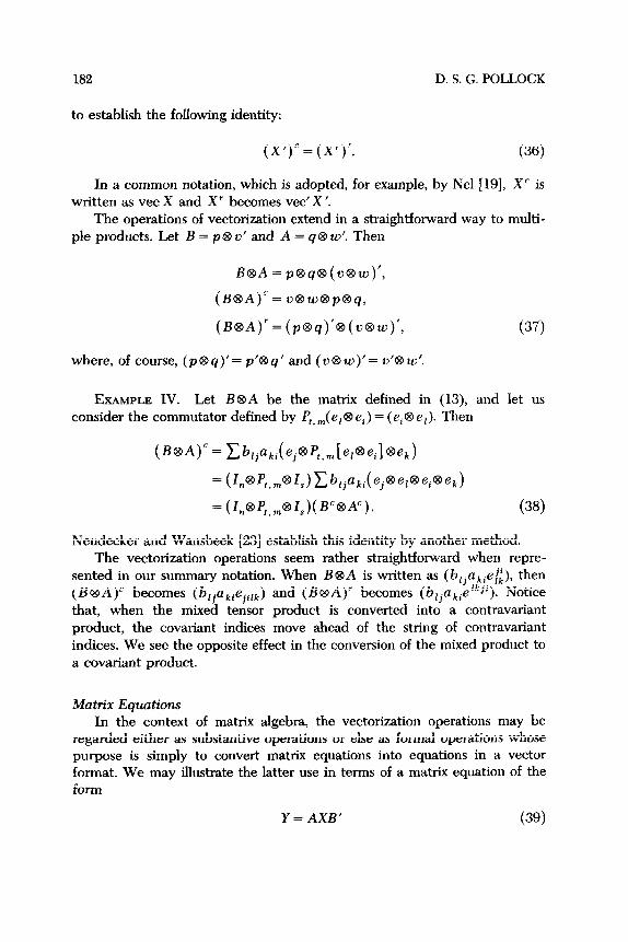
The operations of vectorization extend in a straightforward way to multiple products. Let B = p@ u’ and A = q@ w’. Then

B@A = p@q+mu)‘,

(BQ~A)” = uow8p8q,

(B~A>~ = (p8q)‘~(u~w)‘, (37)

where, of course, (p@q)‘= p’@q’ and (u@w)‘= 0’81~‘.

EXAMPLE IV. Let B@A be the matrix defined in (13), and let us consider the commutator defined by Pt, Je,8 ei) = (e,@ er). Then

(BC+A)“= Cbljaki(ej~Pt,m[erbei]~e~)

= (Z,~P,,,~ZI,)Cbyaki(ej~el~e,~ee,)

= (Z,C+P,,,~ZJ(BC~A~). (38)

Neudecker and Wansbeek [23] establish this identity by another method. The vectorization operations seem rather straightforward when repre-

sented in our summary notation. When B@A is written as ( blja,,ej,!), then (B@A)’ becomes (bljakiejilk) and (B@A)’ becomes (bljakielkji). Notice that, when the mixed tensor product is converted into a contravariant product, the covariant indices move ahead of the string of contravariant indices. We see the opposite effect in the conversion of the mixed product to a covariant product.

Matrix Equations In the context of matrix algebra, the vectorization operations may be

regarded either as substantive operations or else as formal operations whose purpose is simply to convert matrix equations into equations in a vector format. We may illustrate the latter use in terms of a matrix equation of the form

Y = AXB’ (39)

TENSOR PRODUCTS 183

which defines a mapping of X = [xii] in *Y*@7(y into Y = [ykl] in 8*@9, which can be regarded as a decomposable tensor product of the mapping from w to 9, effected by A, and the mapping from Y * to L@*, effected by I?‘. By expressing X in terms of basis vectors, we get

AXB’= A{ &ij(ei@e*j)} f?’

= '&ij(Aei@e*iW).

On applying the row-vectorization operator, we get

(AXIS’)’ = ~xij(e*~se*jB’)

= Cxij(e*ic3e*j)(kc3B’)

= X’(A’@B’).

(40)

(41)

Thus we have the identity

Y’= (AXB’)’

= X’(A’@B’). (42)

This may be described as the covariant representation of the matrix equation. We may apply the column-vectorization operator in an analogous fashion

to obtain the identity

Yc = (AXB’)”

= (B@A)X”. (43)

Alternatively, with an understanding of the rules implied by (42), we can obtain this identity by using the relationship Y” = {(Y ‘)’ }‘.

The identity in (43), which was given by Roth [27] in a paper of 1934, has been rediscovered, at various times, by Aitken [l], Koopmans et al. [13], Nissen [24], and Neudecker [22].

If we are prepared to regard vectorization as a formal operation without substantive implications, then we are able to identify the operation of transposition with that of commutation. Consider the expression

qu’ewy = P(uSw)

=w@u = (W’SU)“. (44


On writing X = 0’8 w, this becomes

PX” = (x’)c; (45)

and we can regard the latter as the transformation mapping X into X’. In fact, Equation (44) is just the vectorized version of Equation (29). Notice also that Equation (29) defines an indecomposable mapping which contrasts with the decomposable mapping defined by Equation (39).

We should note that several authors, including Henderson and Searle [12] and Magnus and Neudecker [17], use Equation (45) as their basic definition of the commutator.

EXAMPLE V. MacRae [16] stated, without proof, the identity

which is given here in the notation of Example II. In our summary notation, C may be written as (cifef), so that C’ is (cifeif). Likewise, A is (akieL), so that A’ is (ukie/) and A” is (ukieki). For I,, I,, I,, and I,, we have (ei), (ei), (e,“), and (e,f) respectively. The identity may be established by writing

( ‘ifelk lkif)( a .d. eljuf

kt ,u lkrf )(b,je;;fuf)=({akicifj(b,jdj,,}e;;f) (47)

and by recognizing that, on the RHS, we have the expression for BD@AC that is given in (23). Rogers [26] has also given a proof of the identity which uses a more traditional algebra and which is, in consequence, rather arduous.

MATRIX DIFFERENTIAL CALCULUS

We shall now use the algebraic results derived in the preceding sections to analyse three alternative definitions of the derivative of the matrix function Y = Y(X) with respect to its matrix argument X. We shall establish relationships amongst the three definitions, and we shall argue that only one of them is viable.

Let Y = [ vkl] be again a matrix of order s X t whose elements are functions of the elements of X = [xi j] of order m x n. Then the definition of the derivative of Y = Y(X) depends upon a choice of a rule whereby we may arrange the mmt elements aYkr/axii in a rectangular matrix. Three altema- tive definitions are in common use.

TENSOR PRODUCTS 185

According to the first definition, the derivative is a partitioned matrix [ JY/&xi j] whose ijth partition is derived from the matrix Y by replacing each element ykl with its derivative ~3y~!/LJx~~. Thus the elements of the matrix derivative have the same disposition as the elements rijykl of the product X@Y. This definition has been studied by Rogers [26] amongst others, and he has ascribed to it the notation &Y/&X. Graham [9] has also adopted it as his basic definition in a recent text.

According to the second definition, the derivative of Y with respect X is a partitioned matrix [ c?Y~~/JX] whose klth partition is derived from the matrix X by replacing the elements r jj with the derivatives Jykr/Jxi j. The elements of the matrix derivative therefore have the same disposition as the elements of Y @ X. This is probably the most commonly used definition. It has been employed extensively by both Rogers [26] and Balestra [2] in their treatises of matrix differential calculus, and it was adopted by MacRae [16] in a seminal article to which many authors have referred.

From another point of view, the two definitions already considered follow directly from the definitions of Dwyer and MacPhail [8], who considered the forms LJY/&x, j and ~?y~//aX without arranging them in partitioned matrices.

According to the third definition, the derivative of Y with respect to X is a matrix JYC/JXr whose elements ayk,/axij have the same arrangement as the elements yklxij in the product Y“@ ( XC)‘. This final definition, which we shall call the vectorial definition, has been used by Neudecker [22] and by the present author [25] amongst many others. Nel [19] has ascribed to this derivative the notation a vet Y/a vet’ X.

The easiest way to reveal the nature of these definitions is to express the derivatives in terms of the natural bases of the associated primal and dual spaces. When Y and X are expressed as

Y = CYkl( ek@e*‘),

X = Cxij(ei@e*j),

it becomes clear that

[ 1 e = C $$ei@ei@e*j@e*l),

aYkr [ 1 7jy = C ~(ekQeic3e*‘c3e*j),

‘I

gi=E$( e,@ee,@e*jc3e*’ 1.

(48)

(49)


The first two derivatives are seen to differ from each other only in respect of the orders within the pair of covariant indices and within the pair of contravariant indices. Thus, using the commutators defined by I’,, ,( e,8 ei) = (ei8ek) and (e*‘@e*j)P,,t = (e*j@e*‘), we can write

and [ f$] = p,:_[ j$&,‘,t. (50)

These are decomposable mappings. The third definition of the derivative aYc/aXc differs from the first two

in a more complicated way which requires the conversion of the basis vectors e, and e *’ into the vectors e*i and e, respectively. These conversions depend upon the use of an indecomposable mapping which has some of the features of the mapping from X to X ’ depicted in (29) and (33).

EXAMPLE VI. The identity

(51)

may be confirmed by examining its expression in terms of our summary notation:

The inverse mapping

e,@Z,@e*') aykl

[ 1 ax (e,@Z,@e*')

(52)

69

may be confirmed in the same way. An alternative expression for the mapping from ayyaxc to [6&&x]

can be obtained by specializing Macrae’s identity, quoted under (46) to give

(Z$Zmc3ZfJ( I,@( &)'cY'@zn~(z:oz,oz,) = Z,YdD (&)Z”

[ I ay,, = ax * (54)

TENSOR PRODUCTS 187

MacDonald [14] has incorrectly identified (a/aX)“Yr with (JYc/aXC)’ to produce his equation (3.12(a)). Nel [19] has provided a correct version of the equation by setting ( a/aX)‘“Yr = P,,,( c?Y’/JX’)‘P~,, in (54). A less tortu- ous version of the identity is

8Yld

[ 1 ax = (z~q@z*) Z,@ g sz, j(z,oz,oz~), i (55)

which may be confirmed by writing it as

(56)

The equation

g = (Z,@Z,OZ~)( I,@ [ $1 @z,)(z;@z,@zm). (57)

which is the inverse of (55), was correctly stated by MacDonald.

EXAMPLE VII. Let Y = [ ykl] and Z = [zfU] be matrix functions of X = [xij]. Then the derivative a(Y@Z)‘/aXc is a matrix whose elements

a(~~~+) aYkl f$u axij = -Zfu + Ytrq axii

have the same arrangement as the elements ykl.zfUxij in the product

(Y@Z)"@(X")'=(z,@P,,,@z,)(Y"@ZC)e(XC)'. (58)

Here the equality is obtained from the identity under (38) in Example IV. The summary notation for this equation is


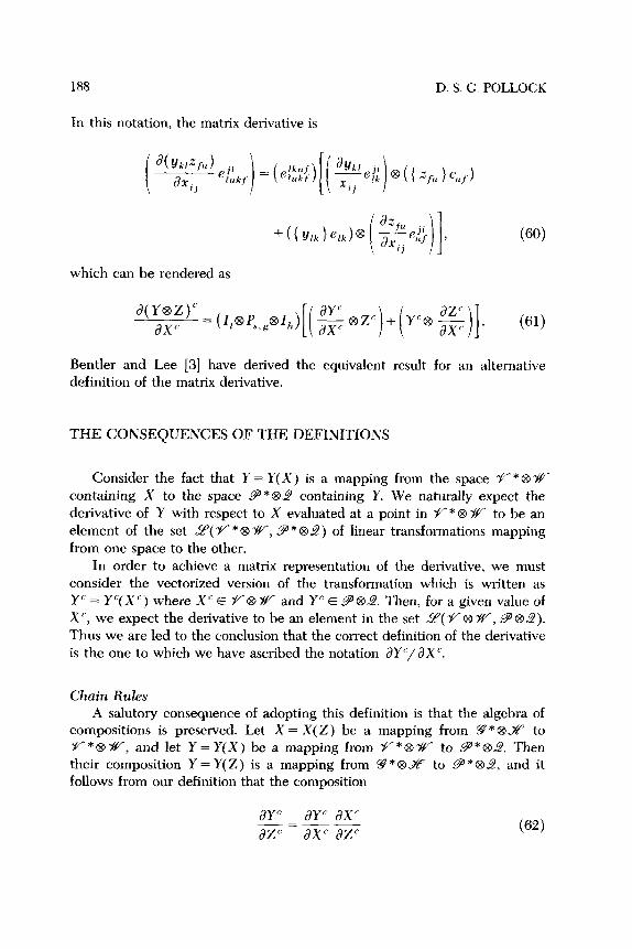
In this notation, the matrix derivative is

which can be rendered as

@Y@Z)”

axr = (4@L,@4)

Bentler and Lee [3] have derived the equivalent result for an definition of the matrix derivative.

THE CONSEQUENCES OF THE DEFINITIONS

I. (61)

alternative

Consider the fact that Y = Y(X) is a mapping from the space ^y_*@ YV containing X to the space 8*@2 containing Y. We naturally expect the derivative of Y with respect to X evaluated at a point in Y *@ +V to be an element of the set 2( V * 8 w, .9’* 822) of linear transformations mapping from one space to the other.

In order to achieve a matrix representation of the derivative, we must consider the vectorized version of the transformation which is written as Y’ = Y’(X’) where X’ E V”@w and Y” E 982. Then, for a given value of X’, we expect the derivative to be an element in the set 5?( V @ z&‘-, 9 ~22). Thus we are led to the conclusion that the correct definition of the derivative is the one to which we have ascribed the notation aYr/aXc.

Chain Rules

A salutory consequence of adopting this definition is that the algebra of compositions is preserved. Let X = X(Z) be a mapping from 9 *8x to V*@w, and let Y=Y(X) be a mapping from V*@ZV to 9*@2. Then their composition Y = Y( 2) is a mapping from 9 *@Z’ to .9 *@2?, and it follows from our definition that the composition

aYc aYc ax< -= -- azc ax“ azr (62)

TENSOR PRODUCTS 189

is a mapping from 98% to 989. Thus we have a chain rule for matrix differential calculus which has been used extensively by MacDonald [14] and the present author [25] amongst many others.

Chain rules obeying the normal algebra of compositions are not available for the other definitions that we have considered.

EXAMPLE VIII. To obtain a chain rule, MacRae [16] was obliged to define a special matrix operation which she called the star product. If X = [x, j] is an m X n matrix and Q = [ Qi j] is an mh X ng partitioned matrix wherein each Q,j is an m X n matrix, then the star product of X and Q is

X * Q = { xxij(ei@e*j)} * ( C4ijf~,(e,8e*jOef~e*11))

(63)

With this definition, it can be asserted that, if y = y(X) is a scalar-valued function of the matrix X = X(Z) which is, in turn, a function of the matrix Z, then

‘“=$K( az a+ ef@e*” >

aY axij =-* - [ 1 ax az ’ (64)

The need to define a star product to replace the usual operation of matrix composition, which suffices for the chain rule defined in (62) is due to the improper conversion of primal basis vectors into dual basis vectors and vice versa in the definition of the derivative that is adopted here.

MacRae’s definition of the star product does not accommodate the case where Y = Y(X) is a matrix function of X = X( Z ). However, we can easily extend the definition to give

(65)


which, in our summary notation, is

(66)

The extended definition has the consequence that

(A’c@B’)*(C’ce~‘)=(AC)‘c@(BD)‘. (67)

This is the expression that we obtain from (65) when Y = AXB’ and X = CZD’. There is no natural way in which the star product may be generalized to

accommodate the composition of mixed tensor products of any higher order.

The Nonconservation of Rank Another fact on which we should comment is that, in certain cases, a

change in the definition of the derivative leads to a change in the rank of its matrix.

Consider again the matrix equation Y = AXB’, which leads to the derivative aYc/aXc = B@A. This matrix has Rank(B@A)= Rank(B)Ra If A is of order m X m and B is of order n X n, and if both are nonsingular, then, as was shown by Deemer and Olkin [7], the Jacobian of the mapping from X to Y is IB@A( = (B(*(A In. The alternative definitions lead to the derivatives [ ay,,/aX] = (A’)C@B’ and [aY/&,,] = A”@(B’)‘. In both cases, we have a matrix which is a decomposable mixed tensor product of two vectors and which, therefore, has rank of unity. The consequence is that we have difficulty in defining the Jacobian.

It is difficult to see how matrix generalizations of the familiar theorems of mathematical analysis which depend upon the concept of the Jacobian matrix -such as the implicit function theory-can be expressed if the vectorial definition of matrix derivatives is not adopted.

CONCLUSION

The process by which we obtain matrix derivatives is frequently referred to as formal or symbolic matrix differentiation. This description alludes to the fact that matrix derivatives are defined without the rigorous mathematical justification that we demand of the underlying theory of scalar derivatives; and it reminds us that our object is to establish a code, or a system of

TENSOR PRODUCTS 191

principles and rules, to assist in the practical task of obtaining and organizing the derivatives. With this in mind, it might be argued that any consistent theory of symbolic matrix derivatives ought to be as good as any other if each is a valid formal representation of the same abstract mathematical relationships. If one accepts the truth of this, then there remains the practical issue of how readily each of the alternative representations can be integrated with contiguous branches of mathematics such as the theory of linear algebra as expressed in matrices or the theory of mathematical analysis. In this paper, we have argued that the vectorial definition of matrix derivatives is the only definition which does not lead to serious disjunctions at such points of contact. We have also suggested that the most efficient way of organizing the accumulating mass of results in the theory of matrix differential calculus is by adopting an elementary theory of the tensor structure of matrices.

AN APPENDIX OF NOTATION

In the following diagram, the letters 9, V, 9, etc. denote vector spaces. The bases of these spaces are indexed by integer arguments U, j, I, etc. which are shown tending to maximum values which are the dimensions of the spaces. The letters D, B, etc. denote transformations from one space to another. The matrices corresponding to the transformations are specified below the diagram.

A = [uki] is an s x m matrix in w*@9,

B= [blj] isatXnmatrixinV*@B,

C=[~~~]isanmXhrnatrixin&‘*@w,

D=[djU]isannXgmatrixin9*@V,

X=[~~~]isanmXnmatrixinV*89V,

Y= [ykl] isan sXt matrixin 9*@2,

Z = [ zr,,] is an h x g matrix in 9*8x.


This paper was written while I was visiting the Faculty of Actuarial Science and Econometrics of the University of Amsterdam. I wish to thank Heinz Neudecker and Roald Ramer, who are members of the Faculty, for helpful discussions. I should also like to thank Gary Keogh and Malcolm MacCallum for their comments and Ingram Olkin for his encouragement.

REFERENCES

7

8

9

10 11

12

13

14

15 16

17

A. C. Aitken, On the Wishart distribution in statistics, Biometrika 36:59-62 (1949).

P. Balestra, La Derivation Matricielle, Sirey, Paris, 1976.

P. M. Bentler and S-Y. Lee, Matrix derivatives with chain rule and rules for simple, Hadamard, and Kronecker Products, J. Math. Psych. 17:255-262 (1978). N. Bourbaki, Algkbre multilinCaire, in El&ments de Mathetnatique, Book II

(Algtibre), Herman, Paris, 1958, Chapter 3. E. Cartan, G&met& des Espaces de Riemann, Gauthier-Villars, Paris, 1952.

H. Chernoff and N. Divinsky, The computation of maxilllurn-likelillood estimates

of linear structural equations, in Studies in Econumetric Method (W. C. Hood

and T. C. Koopmans, Eds., Monograph No. 14, Cowles Foundation for Research in Economics, Yale U.P., New Haven, 1953, Chapter X.

W. L. Deemer and I. Olkin, The Jacobians of certain matrix transformations useful in multivariate analysis, Biometrika 38:345-367 (1951).

P. S. Dwyer and M. S. MacPhail, Symbolic matrix derivatives, Ann. Math. Statist. 19:517-534 (1948). A. Graham, Kronecker Products and Matrix Calculus with Applications, Ellis

Horwood, Chichester, 1981. W. H. Greub, Mu&linear Algebra, Springer, Berlin, 1967. H. V. Henderson and S. R. Searle, vet and vech operators for matrices, with some uses in Jacobians and multivariate statistics, Canad. J. Statist. 7:65-81 (1979).

H. V. Henderson and S. R. Searle, The vet-permutation matrix, the vet operator and Kronecker products: A review, Linear and Multilinear Algebra 9:271-288 (1981). T. C. Koopmans, H. Rubin, and R. B. Leipnick, Measuring the equation systems of dynamic economics, in Dynamic Economic Models (T. C. Koopmans, Ed.), Monograph No. 10, Cowles Foundation for Research in Economics, Wiley, New

York, 1950, Chapter 2. R. P. MacDonald, The MacDonald-Swaminathan matrix calculus: Clarifications, extensions and illustrations, General Systems 21:87-94 (1976). C. C. MacDuffee, The Theory ofMatrices, Springer, Berlin, 1933. E. C. MacRae, Matrix derivatives with an application to an adaptive linear

decision problem, Ann. Statist. 2:337X46 (1974). J, R. Magnus and H. Neudecker, The commutation matrix: Some properties and

applications, Ann. Statist. 7:381-394 (1979).

TENSOR PRODUCTS 193

18 M. Marcus, Finite Dimensional Multilinear Algebra-Part I, Marcel Dekker, New York, 1973.

19 D. G. Nel, On matrix differentiation in statistics, South African Statist. J.

14:137-193 (1980). 20 H. Neudecker, On matrix procedures for optimizing differentiable scalar func-

tions of matrices, Statist. Neerlandica 21:101-107 (1967). 21 H. Neudecker, The Kronecker product and some of its applications in economet-

rics, Statist. Neerlandica 22:69-82 (1968). 22 H. Neudecker, Some theorems on matrix differentiation with special reference to

Kronecker matrix products, J. Amer. Statist. Assoc. 64:953-963 (1969). 23 H. Neudecker and T. J. Wansbeek, Some results on commutation matrices, with

statistical applications, Canad. J. Statist. 11:221-231 (1983). 24 D. H. Nissen, A note on the variance of a matrix, Econometrica 36:603-604

(1968).

25 D. S. G. Pollock, The AZgebra of Economelrics, Wiley, Chichester, 1979. 26 G. S. Rogers, Matrix Deriuatiues, Marcel Dekker, New York, 1980.

27 W. E. Roth, On direct product matrices, Bull. Amer. Math. Sot. 40:461-468 (1934).

28 A. Zellner, An efficient method of estimating seemingly unrelated regression

equations and tests for aggregation bias, J. Amer. Statist. Assoc. 57:348-368 (1962).

Rewiced 30 September 198.3; recised 6 Septmdwr I981

d. s. g. pollock department of economics queen …. s. g. pollock department of economics queen mary...

Documents