school · pdf filean analysis of public school expenditures in ohio reveals that ... center,...

A STUDY BY THE OHIO SCHOOL BOARDS ASSOCIATION

JANUARY 2011

SCHOOLCONSOLIDATION

1

The current ! nancial climate across the country has led to increased interest

in school district consolidation as a means to improve e" ciencies and save

money in the operation of public school districts. However, the evidence

concerning the actual resulting savings from school district consolidation is

mixed at best. An analysis of public school expenditures in Ohio reveals that

while small school districts may spend more dollars per pupil on administrative

expenses, they actually spend less per pupil on total expenditures, with no

loss in quality of educational outcomes. Shared services and purchasing

cooperatives appear to be a more promising approach to saving money while

preserving a sense of community identity.

2

School consolidation — A framework for discussionSchool consolidation and merger account for the most dramatic change in educational governance and management in the United States in the twentieth century. Since 1937, the number of school districts has declined from 117,000 to fewer than 14,000 in 2007, a reduction of more than 95% (National Center for Educational Statistics, 2009). At that time, the pupil enrollment in the United States was 25.4 million and the average enrollment per building was approximately 102 pupils. In 1997, pupil enrollment was 45.6 million and the average enrollment per building was nearly 496.

Even though the pace of consolidation has slowed over the recent past, school consolidation continues to occur every year. It is likely to remain on the education policy agenda as states face continuing revenue pressures and demands to reduce taxes. School consolidation continues to be a focus of national discussion based on two premises:• saving money,• improving student achievement.

Consolidation can be a very controversial topic for policymakers, school boards and administrators, as well as for the communities involved. The perceived economic advantages must be balanced with many perceived social disadvantages. Emotions can run high and deep, and old memories may linger for years.

Nationally, there are 12 states with initiatives or legislative mandates concerning merger and consolidation. Among these states, four are clearly targeting merger to eliminate small schools with the goal of saving money. According to a study by the Pennsylvania School Boards Association (2009), there is active legislation in several states, including Indiana, Illinois, Kansas, Maine, Massachusetts, Michigan, New York, Oregon, Pennsylvania, Washington, West Virginia and Wisconsin. The goals of the legislation are as follows:• eliminate small school districts,• eliminate small school districts/buildings with fewer than 350 students,• combine elementary and secondary districts into K-12 districts,• reduce the number of districts.

One state seeks to encourage consolidation by providing economic incentives for districts that consolidate, while two will impose penalties for districts that fail to consolidate. In 2007, Maine directed its 290 school districts to consolidate into 80 regional school units. To date, only 27 regional school units have been created and local voters rejected merger in 180 other districts.

Locally, “Restoring Prosperity: Transforming Ohio’s Communities for the Next Economy,” a report issued in February 2010 by the Brookings Foundation and the Greater Ohio Policy Center, has triggered discussions about school consolidation in Ohio. One of the 39 recommendations in the report called for a reduction by one-third in the number of Ohio

public school districts. The report called for no district to have fewer than 2,500 pupils. Of Ohio’s 613 school districts, 410, or two-thirds enroll

fewer than 2,500 pupils. The recommendation has been embraced by a number of politicians at the state level who appear to believe that it o# ers a quick way to save dollars.

Let us turn to an examination of the two premises underlying calls for consolidation.

3

SAVING MONEY

The potential to save money is based on the reduction or elimination of duplicated services and taking advantage of economies of scale. When consolidation is considered, cost projections usually suggest potential savings. However, few post-consolidation studies document actual savings. An analysis of school consolidation results published by the Fordham Institute (2003) states that “consolidation promises lower costs and taxes and better student performance, but neither happens.”

Projected savings often overlook higher costs that result from “leveling up of sta# salaries,” additional transportation costs and front-end costs associated with the transition. Such front-end costs include the need for new textbooks and curriculum materials, issues related to integrating computer software, legal costs to address contractual issues and costs for new signage, athletic and band uniforms, and stationery, among others. While these may be small costs individually, they become large when aggregated.

Studies reported from 1960 through 2004 fail to show any conclusive evidence that consolidation of small districts necessarily reduces ! scal expenditures on a per-pupil basis. In addition, school consolidation can often result in school closures, leading to negative economic impact on the community.

The size of the districts involved in the consolidation process appears to have a relationship to savings realized. Based on a study of school consolidation e# orts in New York, Duncombe and Yinger (2001) conclude that consolidation may lower the costs of two consolidated 300-pupil districts by over 20%; may lower the costs of two consolidated 900-pupil districts by 7% to 9%; but have little, if any, impact on the costs of two 1,500-pupil districts.

IMPROVING STUDENT ACHIEVEMENT

The potential to improve student achievement is based on the belief that a larger district can provide more varied opportunities for students. However, again the research shows mixed results. The actual impact on student achievement appears to be mediated by other factors, such as the demographics of the populations involved. For example, in a study of consolidation results in Arkansas, Howley (1994) noted that small schools serving high-poverty areas actually produce higher student achievement than larger consolidated schools. Other studies have suggested that students going from a small school to a larger school su# er isolation and disconnect and may not participate in as many cocurricular opportunities. Studies conducted in Pennsylvania have found an adverse impact on academic achievement and a sense of loss of community in consolidated districts. Local choice is the critical element in the process.

According to Raywid (1999), when viewed strictly on a cost-per-pupil basis, small schools may be somewhat more expensive, but when viewed on the basis of bene! ts, such as the percentage of graduates, they are less expensive. Cotton (1999) lists several advantages of small schools — including higher achievement, better attitudes toward school, fewer social behavioral problems, higher extracurricular participation, higher attendance and lower dropout rates.

Local choice appears to be the critical element in determining the ultimate outcome of school consolidation e# orts. Forced or mandated consolidation often leaves feelings of disenfranchisement and bitterness that can span generations. A recent Columbus Dispatch editorial noted “true consolidation would pose many hurdles, starting with the fact that Ohioans place a high value on local control of schools. Pride in local schools runs deep, so any e# ort by the state to eliminate wasteful duplication will be doomed to fail if it tries to force consolidation.”

Nationally, there are 12 states

with initiatives or legislative

mandates concerning merger and consolidation.

4

Shared services in Ohio — An alternative approachSchool districts have long seen the bene! ts of collaboration instead of consolidation. Sharing resources and enacting joint purchasing agreements across regions can have the same advantages as consolidation, while allowing each school community to maintain its own identity (Darden, 2005). Examples include building use, transportation, schedules, personnel, technology and attendance. Ohio schools have been using such concepts for many years. Educational service centers and regional school district purchasing cooperatives o# er school districts many opportunities to realize cost-savings by economies of scale in purchasing. At the state level, the professional management organizations — the Ohio School Boards Association, Buckeye Association of School Administrators and Ohio Association of School Business O" cials — o# er pooling and group purchasing for insurance, worker’s compensation and electricity that result in signi! cant savings for Ohio school districts.

There are also examples of school districts sharing sta# for specialized programs, such as low-incidence handicapped pupils. Two districts in Ohio — Orrville City and Rittman Exempted Village — currently share a treasurer and superintendent. As school funding continues to pose di" culties, it is likely that more and more districts will search for such creative approaches.

CONSOLIDATION IN OHIO

School consolidation is not a new concept in Ohio. The number of public school districts has declined from 2,674 in 1915 to 613 today. The peak of consolidation in Ohio occurred during the 1950s when the legislature o# ered incentives to small districts to merge or consolidate.

In Ohio, school districts are political subdivisions created by the legislature to carry out the constitutional mandate to provide a thorough and e" cient system of public elementary and secondary schools. Therefore, the procedures for creating, dissolving and consolidating school districts are provided exclusively by the legislature.

The legislature has provided for various types of territorial changes. Speci! c procedures are identi! ed for each type (RC 3311.22). In general, the process can be initiated by action of a board

of education seeking to transfer territory, by a petition signed by a set percentage of the quali! ed electors residing in the a# ected portion of the school district, by

proposal of the State Board of Education or by agreement of the districts involved in municipal annexation.

ACHIEVEMENT RESULTS IN OHIO BY DISTRICT ENROLLMENT

Table 1 at right displays the state report card rating by school district size for the 2009-2010 school year. School districts have been

grouped into six enrollment bands: Less than 1,250; 1,251-2,500; 2,501-3,750; 3,751-5,000; 5,001-7,500; and greater than 7,500. The report card ratings are Excellent with Distinction, Excellent, E# ective, Continuous Improvement, Academic Watch and Academic Emergency.

5

The smallest Ohio school districts, those with enrollments up to 2,500 pupils, account for nearly 70% of all Ohio districts. They account for 190 of the 296 districts earning an Excellent or Excellent with Distinction rankings, and 196 of the 240 E# ective districts. They account for 65% of the Excellent/Excellent with Distinction districts and 82% of the E# ective districts. When combined, the small school districts account for 72% of all districts performing in the top three categories. This indicates that the academic performance of students enrolled in small school districts is proportionate to their representation in the total pupil population. In other words, when considering school district size alone, attending a small school district produces equal or better academic results.

An earlier study prepared by the Ohio Public Expenditure Council (2007) examined the characteristics of the 25 largest and 25 smallest school districts. Among the ! ndings, the average graduation rate for the largest districts was 84.7% compared to 96.4% for the smallest districts. The di# erence for attendance rates was less dramatic, with the large district average at 94.5% compared to 96.4% for the small districts. The authors noted that other signi! cant intervening variables, such as poverty rate, may account for the di# erences noted.

DISTRICT SIZE AND PUPIL EXPENDITURES

The Ohio School Boards Association initiated a research project to better understand the relationship between school district size and expenditures. The study was conducted with the assistance of Howard Fleeter and William Driscoll, respected experts in the area of school ! nance. The results of that analysis follow.

ANALYSIS OF SCHOOL DISTRICT SIZE RELATIVE TO OTHER DATA ABOUT SCHOOL ADMINISTRATION AND SPENDING

Following are the results of an analysis of the size of school districts, as measured by average daily membership (ADM), in the context of other variables about school operations or funding. The analysis attempted to ! nd relationships between school district size and the costs of delivering education services. Some public policy advocates contend that “small” school districts operate with ine" ciencies relative to other school districts of larger size. In this context, “small” refers to the size of a district’s student enrollment or ADM rather than to the geographical size of a district as measured by square miles or some similar method.

Table 1. School District Report Card rating by enrollment

Note that the total of 610 does not contain the island districts or College Corner LSD.

enrollment Academic Emergency

Academic Watch

ContinuousImprovement

E! ective Excellent Excellent with Distinction

totals

< than 1,250 0 2 18 96 63 18 197

1,251-2,500 0 1 17 100 80 29 227

2,501-3,750 0 2 13 24 33 11 83

3,751- 5,000 0 1 3 9 16 9 38

5,001-7,500 1 1 7 9 12 8 38

> than 7,500 0 2 6 2 11 6 27

Totals 1 9 64 240 215 81 610

…the average graduation rate for the largest

districts was 84.7% compared

to 96.4% for the smallest districts…

6

If school districts maintain small enrollment, theoretically, they cannot provide as e" cient a public service as school districts with larger enrollment. The solution to this problem would be to combine two or more “small” school districts or attach a “small” district to a larger district. The advantage claimed for such district consolidation would take the form of improved e" ciency by achieving economies of scale.

A frequent example used to illustrate the ine" ciency of “small” school districts points to the savings inherent in the elimination of unnecessary superintendent and school treasurer positions. However, these examples o# er only anecdotal indications of potential savings. This paper attempts to examine the costs in school districts of di# erent sizes in order to relate those costs to the size of school districts in a more comprehensive manner.

DATA AND METHODOLOGY

The data used in this analysis come from three sources within the Ohio Department of Education (ODE):

1) An annual report of school district ! nances popularly known as the “Cupp Report,” as published by ODE for ! scal year (FY) 2009;

2) Data about the number of school buildings per school district provided by ODE for computation of the Evidence-Based Model (EBM) used in the determination of state school aid in FY10 and FY11 and based on data collected for the school year ending in FY08 or FY09;

3) Data about the percentage of pupils in poverty by school district as reported on school district report cards for FY08.

The analysis ranked school districts from smallest to largest in enrollment (as de! ned by ADM). It then divided the districts into six di# erent classes based on size. (A description of the method for de! ning the classes follows shortly.) A comparison related various characteristics of school district operations or expenditures to the classi! cations based on school district size. Speci! cally, these comparisons attempted to identify patterns by which small school districts tended to show higher relative reliance on administrators, administrative costs or higher costs in general.

The analysis excluded the island districts (Middle Bass, Kelleys Island, Put-in-Bay), as well as College Corner due to their exceedingly small size, and Manchester (Adams County) due to a lack of complete data.

DEFINITION OF SCHOOL DISTRICT SIZE

Identi! cation of “small” school districts requires some objective method for evaluating district size. Fortunately, the state evidence based funding model (EBM) provides exactly such a tool. Various elements of the EBM fund schools based on the number of organizational units contained in them. The EBM de! nes three organizational units as follows.

An organizational unit de! nes a conceptual entity useful for determining state aid amounts. It does not necessarily have a separate existence as a physical building. For example, a school district could have a school with grades six through 12 under one roof. If that school’s enrollment had 557 middle school pupils and 733 high school pupils, the funding formula would credit two organizational units, even if the district housed those units in one building.

type of school enrollment

Elementary - Grades K through ! ve 418

Middle - Grades six through eight 557

High - Grades nine through 12 733

Table 2: Classi! cation of organizational units under the EBM

An organizational unit de! nes a

conceptual entity useful for

determining state aid amounts.

7

The model school sizes de! ned by the EBM suggest a method for estimating the size of a model school district. Table 3 shows the math.

Table 3: Model school district as implied by the EBM

type of school enrollment per unit

number of units

enrollmentper grade

totalenrollment

Elementary - Grades K through ! ve 418 3 209 1,254

Middle - Grades six through eight 557 1 186 557

High - Grades nine through 12 733 1 183 733

All Grades 196 2,544

The table shows that three elementary schools of “model” size would serve a total enrollment of 1,254 in six grades. One middle school and one high school of model size would enroll 1,290 pupils in seven grades. The numbers prescribed for the de! nition of organizational units do not ! t perfectly because they are based on statewide averages of di# erent combinations of enrollment derived from 608 school districts (the 613 school districts minus the ! ve districts noted above). However, it is clear that the elementary grades must promote a su" cient number of pupils each year to sustain the requisite enrollment envisioned by the EBM at the middle and high school levels. Three elementary units at 418 pupils per unit provides an approximate total in order to populate the upper grades consistently with the model. Since some attrition tends to occur in later grades, the slightly larger annual cohorts in early years are consistent with somewhat smaller enrollments in later grades.

If the total enrollment for each model district were rounded down to 2,500, the following classi! cation of school districts according to multiples of that size becomes possible. Table 4 presents this classi! cation system. Note that neither an enrollment of 2,544 nor one of 2,500 has any formal status in the law governing the EBM. The district amount of 2,544 represents a reasonable inference based on the enrollment amounts used to establish the computation of organizational units in the model. The adjustment of the total from 2,544 to 2,500 simply provides a more intuitively easy mathematical structure for evaluating the results of the analysis. (Note that the model district size of 2,500 pupils implied by the EBM is greater than the “optimal district size” of 1,500 students referred to in footnote #164 of the 2010 Brookings Institute report “Restoring Prosperity: Transforming Ohio’s Communities for the Next Economy.” In this light, the EBM model district size appears to be much more realistic than that referenced by Brookings.)

Table 4: Classi! cation of school district by enrollment in multiples of a model school district with 2,500 pupils - 2009 ADM

multiple of 2,500 district enrollment number of school districts

1. one-half or less 0 to 1,250 192

2. one-half to one 1,250 to 2,500 218

3. one to one and one-half 2,500 to 3,750 80

4. one and one-half to two 3,750 to 5,000 46

5. two to three 5,000 to 7,500 38

6. more than three More than 7,500 34

total number of districts 608

Table 4 presents six classi! cations of school districts. The classi! cations rely on the “model” school district size developed from the EBM in Table 3. Class #1 contains those school districts where total enrollment equals one-half or less of the model enrollment of 2,500. Class #2 includes those

Three elementary units at 418

pupils per unit provides an

approximate total in order to

populate the upper grades

consistently with the model.

8

districts where enrollment equals more than one-half of the model amount, but less than the model amount itself. The other four classes follow a similar pattern by using multiples of the model amount. The second column of the table makes the enrollment range for each classi! cation explicit. The ! nal column shows the number of school districts within each classi! cation.

Table 4 shows that 192 school districts have enrollment less than one-half of the model number of 2,500. Another 218 school districts have enrollment from one-half to one times the model size. This means that about two-thirds of Ohio school districts have no more than the enrollment benchmark (410 of 608). (Since no district has an ADM of exactly 2,500, the 410 school districts all have an enrollment less than the benchmark.) Furthermore, almost one-third of all school districts have an enrollment no more than one-half of the size of the model district.

Results of the analysis will use the district classi! cations shown in Table 4 to identify relationships between school districts within each class and data about school operations and funding.

Table 5 expands the basic count of school districts in each size grouping in Table 4 by showing the number of school districts in each ODE District Typology category within each size group.

Each row in Table 5 shows the school districts within the enrollment range displayed in the ! rst column. The following columns show the number of districts within that size range. For example, the ! rst row of data show the very small school districts, districts with less than one-half of the enrollment implied by the EBM. The ! rst column of data shows that ODE assigns 41 very small school districts to its Typology 1.

A complete description of the ODE typology groupings appears in Appendix 2, however, in abbreviated form, the ODE typology sorts districts into the following groups:

#1 - Rural/agricultural with high poverty#2 - Rural/agricultural with low poverty

districtenrollment type #1 type #2 type #3 type #4 type #5 type #6 type #7 total

0 to 1,250 41 91 30 19 0 10 1 192

1,250 to 2,500 42 62 40 34 0 32 8 218

2,500 to 3,750 10 7 8 24 1 20 10 80

3,750 to 5,000 3 1 2 14 0 19 7 46

5,000 to 7,500 0 0 1 10 3 16 8 38

more than 7,500 0 0 0 1 11 10 12 34

total 96 161 81 102 15 107 46 608

Table 5: School districts sorted according to enrollment and by ODE district typology - 2009 ADM

Almost one-third of all school

districts have an enrollment no

more than one-half of the size of the model district

districtenrollment type #1 type #2 type #3 type #4 type #5 type #6 type #7

0 to 1,250 21% 47% 16% 10% 0% 5% 1%

1,250 to 2,500 19% 28% 18% 16% 0% 15% 4%

2,500 to 3,750 13% 9% 10% 30% 1% 25% 13%

3,750 to 5,000 7% 2% 4% 30% 0% 41% 15%

5,000 to 7,500 0% 0% 3% 26% 8% 42% 21%

more than 7,500 0% 0% 0% 3% 32% 29% 35%

Table 6: Percentage of districts sorted according to size assigned to each ODE typology - 2009 ADM

9

#3 - Rural/small town with moderate to high income#4 - Urban with low income#5 - Major urban#6 - Urban/suburban with high income#7 - Urban/suburban with very high income

Table 6 shows the percentage of each size grouping assigned to each ODE typology. For example, 21% of the very small districts appear in Typology 1. Another 47% of the very small districts appear in Typology 2. Another 16% of the very small districts receive a Typology 3 designation. Thus, these ! rst three categories characterize 84% of the districts 1,250 pupils or fewer.

At the other end of the table, 96% of the large districts (7,500+ pupils) appear in Typologies 5, 6 and 7.

These data should not cause much surprise. Intuitively, rural districts have low pupil density and low enrollment. Urban districts have high pupil density and large enrollments. Tables 5 and 6 simply document what reasonable expectations would imply.

RESULTS

The following tables continue to order school districts according to their enrollment. The average experience of di# erent variables relative to size appears in each table.

A. Pupil/administrator ratio

The Cupp Report data set provides data on the ratio of pupils to full time equivalent (FTE) administrators for each school district. This data is based on the EMIS O" cial/Administrative sta# data (category 100 positions). A description of these positions appears in Appendix 1 to this report.

Table 7 shows the ratio of pupils to administrators according to school district size. The table shows a consistent pattern by which the average number of pupils per administrator increases as the size of the districts increases. For example, in row 1, the table shows that very small districts have 120 pupils per administrator. The ratio increases in the model school district size (2,500 to 3,750) to about 175 pupils per administrator.

Table 7 also shows the range within each size group from the minimum ratio of pupils to administrators to the maximum ratio of pupils to administrators. This information appears in the ! nal three columns of the table. Generally, a wide variance exists within each group. In other words, any two given school districts within a given enrollment category can vary signi! cantly in terms of the ratio in each district of pupils to administrators.

Table 7: Average ratio of pupils to administrators according to school district size and minimum, maximum and ratio range within each school district size group

districtenrollment

average ratio: pupils to administrators

FTE

minimumratio

maximumratio

ratiorange

number of districts

0 to 1,250 120 37 265 227 192

1,250 to 2,500 149 42 265 223 218

2,500 to 3,750 175 81 278 197 80

3,750 to 5,000 180 82 309 227 46

5,000 to 7,500 189 126 285 159 38

more than 7,500 206 105 300 194 34

statewide average 159 608

The Cupp Report data set provides

data on the ratio of pupils

to full time equivalent (FTE) administrators for each school

district.

10

Table 7 shows that small school districts have fewer pupils per administrator than larger school districts. Each administrator in the larger districts manages operations for more pupils than do administrators in the small district. The range of the ratio within each size classi! cation appears much greater in small districts. However, Table 7A presents a somewhat di# erent picture. This table eliminates outliers in each size classi! cation. The result shows that the average pupil-to-administrator ratio within each classi! cation does not change much when outliers are removed. However, the ratio range in each classi! cation becomes much closer.

Table 7A: average ratio of pupils to administrators according to school district size and minimum, maximum and ratio range within each school district size group for the 5% to 95% range within each group

districtenrollment

average ratio: pupils to administrators

FTE

minimumratio

maximumratio

ratiorange

number of districts

0 to 1,250 118 62 186 124 174

1,250 to 2,500 148 89 212 123 198

2,500 to 3,750 175 118 237 119 72

3,750 to 5,000 179 120 278 158 42

5,000 to 7,500 188 128 271 144 36

more than 7,500 206 139 268 129 32

statewide average 164 554

The exclusion of extremely low- and high-ratio districts brings the ratio range much closer together among the groups of districts. The number of districts in the last column shows how many districts remain in each size category after the lowest and highest 5% of the districts in that category (the outliers) are removed. These remaining districts from the ! fth to 95th percentile (known as the “federal range”) provide the basis for the results shown in the other four columns of data on the table.

Since the number of administrators used in the computation of this ratio includes principals, the smaller ratio of pupils to administrators in small districts may re$ ect smaller school sizes rather than over-sta# ed central o" ces. The number of schools in a district and, therefore, the need for principals, can result from geographical dispersion characteristic of many smaller districts.

11

B. Expenditures per pupil for di" erent purposes

The following 12 tables summarize the expenditure-per-pupil data about the school districts in di# erent size categories in pairs. The presentation is similar to the approach in Tables 7 and 7A. The ! rst table of each pair shows the results for all school districts. The second table presents the federal range for each size category by showing the results obtained after the removal of outliers at the high and low end of each size category.

The Cupp Report presents expenditure data according to the following categories. Information on the ODE website provides a de! nition for each expenditure item. All of the de! nitions come from the 2009 State Report Card database.

• Administration expenditure per pupil covers all expenditures associated with the day-to-day operation of the school buildings and the central o" ces as far as the administrative personnel and functions are concerned. Items of expenditure in this category include salaries and bene! ts provided to all administrative sta# , as well as other associated administrative costs.

• Sta! support expenditure per pupil includes all the costs associated with the provision of support services to school districts’ sta# . These include in-service programs, instructional improvement services, meetings, payments for additional training and courses to improve sta# e# ectiveness and productivity.

• Building operation expenditure per pupil covers all items of expenditure relating to the operation of the school buildings and the central o" ces. These include the costs of utilities and the maintenance and the upkeep of physical buildings.

• Pupil support expenditure per pupil includes the expenses associated with the provision of services other than instructional that tend to enhance the developmental processes of the students. These cover a range of activities, such as student counseling, psychological services, health services, social work services, etc.

• Instructional expenditure per pupil includes all the costs associated with the actual service of instructional delivery to the students. These items strictly apply to the school buildings and do not include costs associated with the central o" ce. They include the salaries and bene! ts of the teaching personnel and the other instructional expenses.

• Total expenditure per pupil is the combination of all of the components of expenditure listed above.

Data presented in the following tables do not account for expenditures and services provided by educational service centers (ESCs). ESCs achieve economies of scale by providing services to smaller school districts. Their programs could ! t into any of the ! ve categories of expenditure presented in the following tables. ESCs deliver services to school districts accounting for over 1.3 million pupils at a total base cost to the state and school districts of about $42 per pupil.

Table 8 tends to con! rm the notion that the smallest districts operate with the least administrative e" ciency. Row 1 of the table shows that the very small districts spend $1,265 per pupil on administration, while the medium range districts (2,500 to 3,750) spend the least amount per pupil at $1,102.

In fact, the districts grouped around the model enrollment level also have the best expenditure-per-pupil ratio. The last three columns of the table show that the greatest variance in administrative expenditures per pupil occurs in the smallest districts. The variance is inversely related to district size, decreasing as districts get larger. This relationship probably results because a small di# erence in the number of administrators could make a relatively large di# erence in the average expenditure per pupil.

…the districts grouped around

the model enrollment level

also have the best expenditure-

per-pupil ratio.

12

Table 8: Average administration expenditures per pupil according to school district size

districtenrollment

average administration

expense per pupil

minimumexpenseper pupil

maximumexpenseper pupil

expenserange

per pupil

number of districts

0 to 1,250 $1,265 $676 $3,368 $2,692 192

1,250 to 2,500 $1,127 $686 $2,702 $2,016 218

2,500 to 3,750 $1,102 $746 $2,557 $1,811 80

3,750 to 5,000 $1,130 $824 $2,411 $1,587 46

5,000 to 7,500 $1,216 $696 $2,131 $1,435 38

more than 7,500 $1,183 $795 $1,744 $949 34

statewide average $1,196 608

Table 8A: Average administration expenditures per pupil according to school district size and minimum, maximum and administrative expenditure per pupil range within each school district size group for the 5% to 95% range within each group

districtenrollment

average administration

expense per pupil



expenserange

per pupil

number of districts

0 to 1,250 $1,237 $928 $1,781 $853 174

1,250 to 2,500 $1,105 $839 $1,496 $657 198

2,500 to 3,750 $1,077 $825 $1,508 $683 72

3,750 to 5,000 $1,104 $898 $1,519 $621 42

5,000 to 7,500 $1,205 $778 $1,978 $1,200 36

more than 7,500 $1,177 $815 $1,739 $924 32


Table 8A shows that the elimination of outliers reduces the per-pupil expenditure ranges. This suggests that a serious analysis of administrative costs might ! rst address the outliers in each

group to determine why those districts registered unusually high or low expenditures per pupil for administrative costs.

13

Table 9 suggests that the relationship between size and e" ciency is more complicated than the data in Table 7 might imply. While very small districts in Row 1 of Table 8 spend $69 more per pupil on administration than the statewide average expenditure per pupil and about $100 more per pupil than the average of the districts in the other ! ve size classi! cations, these same districts spend $177 less per pupil on sta# support expenditures than the statewide average.

Table 9: Average sta" support expenditures per pupil according to school district size

districtenrollment

average sta! support expense

per pupil



per pupilexpense

range

number of districts

0 to 1,250 $153 $9 $852 $843 192

1,250 to 2,500 $197 $0 $1,036 $1,036 218

2,500 to 3,750 $225 $10 $1,118 $1,108 80

3,750 to 5,000 $274 $40 $755 $715 46

5,000 to 7,500 $369 $58 $779 $721 38

more than 7,500 $453 $89 $940 $851 34

statewide average $330 608

Removal of outliers from the results in Table 9 does not change the overall picture. Smaller districts spend less on sta# support in a consistent pattern even after the exclusion of extremes. Table 9A shows these results. However, the removal of outliers does reduce the range of expenditures dramatically in the small district categories.

Table 9A: Average sta" support expenditures per pupil according to school district size and minimum, maximum and administrative expenditure-per-pupil range within each school district size group for the 5% to 95% range within each group

districtenrollment

average sta! support expense per

pupil



expenserange

per pupil

number of districts

0 to 1,250 $141 $26 $396 $370 174

1,250 to 2,500 $183 $13 $540 $527 198

2,500 to 3,750 $213 $26 $448 $422 72

3,750 to 5,000 $264 $62 $606 $544 42

5,000 to 7,500 $366 $64 $760 $696 36

more than 7,500 $449 $116 $928 $812 32

statewide average $324 554

For example, the second and third rows of data on Table 9 show ranges of expenditures in excess of $1,000 per pupil. After the exclusion of outliers, the range in the second row shrinks to just $527 and in the third row to just $422. Most of the change from Table 9 to 9A occurs because one or two districts in these categories spend a lot of money on sta# support relative to other districts in those size categories and relative districts generally.

14

Table 10 shows the results for building and operations expenditures. Average expenditures do not vary much among the size classes. Large districts tend to spend a little more per pupil than the small districts for building and operations. The largest e# ect caused by removal of outliers again appears in the range of expenditures. A few high expenditure districts cause the large range of expenditures in most cases. Data about speci! c districts show that Lordstown LSD spent over $5,500 per pupil. It is possible that this very unusual expenditure re$ ects a one-time maintenance expenditure rather than a continuing commitment to operations costs at that high level. Similar explanations might explain some of the other unusual results in this category.

Table 10: Average building & operations expenditure per pupil according toschool district size

districtenrollment

building & operations expense

per pupil



expenserange

per pupil

number of districts

0 to 1,250 $1,888 $904 $5,513 $4,609 192

1,250 to 2,500 $1,890 $1,072 $4,472 $3,400 218

2,500 to 3,750 $1,807 $1,121 $2,723 $1,602 80

3,750 to 5,000 $1,959 $1,293 $3,154 $1,861 46

5,000 to 7,500 $2,056 $1,426 $3,961 $2,535 38

more than 7,500 $2,074 $1,461 $3,469 $2,008 34


Comparison of Table 10A to Table 10 shows that the removal of the outliers brings the minimum and maximum expenditure results closer to the average.

Table 10A: Average building & operations expenditure per pupil according to school district size and minimum, maximum and administrative expenditure-per-pupil range within each school district size group for the 5% to 95% range within each group

districtenrollment

building & operations expense

per pupil



expenserange

per pupil

number of districts

0 to 1,250 $1,844 $1,288 $2,584 $1,296 174

1,250 to 2,500 $1,857 $1,397 $2,563 $1,166 198

2,500 to 3,750 $1,800 $1,411 $2,287 $876 72

3,750 to 5,000 $1,941 $1,502 $2,706 $1,204 42

5,000 to 7,500 $2,021 $1,471 $3,018 $1,547 36

more than 7,500 $2,050 $1,621 $2,989 $1,368 32


Large districts tend to spend

a little more per pupil than the small districts

for building and operations.

15

Tables 11 and 11A present data about pupil support expenditures. As with sta# support, average per pupil support expenditures increase directly in relation to district size.

Table 11: Average pupil support expenditure per pupil according to school district size

districtenrollment

pupil support expense per pupil



expenserange

per pupilnumber of

districts

0 to 1,250 $894 $367 $3,448 $3,081 192

1,250 to 2,500 $911 $430 $2,505 $2,075 218

2,500 to 3,750 $943 $406 $1,835 $1,429 80

3,750 to 5,000 $1,052 $584 $1,905 $1,321 46

5,000 to 7,500 $1,143 $593 $2,075 $1,482 38

More than 7,500 $1,154 $679 $1,733 $1,054 34


A few high expenditure districts increase the range of per-pupil expenditures in the small districts. The removal of these outliers decreases the range of per-pupil expenditures for pupil support. Table 11A shows the tighter range caused by smaller di# erences in expenditures after exclusion of extremes.

Table 11A: Average pupil support expenditure per pupil according to school district size and minimum, maximum and administrative expenditure-per-pupil range within each school district size group for the 5% to 95% range within each group

districtenrollment

pupil support expense per pupil



expenserange

per pupil

number of districts

0 to 1,250 $865 $535 $1,357 $822 174

1,250 to 2,500 $884 $510 $1,441 $931 198

2,500 to 3,750 $929 $623 $1,356 $733 72

3,750 to 5,000 $1,038 $670 $1,602 $932 42

5,000 to 7,500 $1,132 $668 $1,801 $1,133 36

more than 7,500 $1,151 $807 $1,678 $871 32


The two categories with the smallest districts spend about $250 to $280 less for pupil support than the two categories of largest districts.

16

Tables 12 and 12A show data about instructional expenditures per pupil.

The two categories with the smallest districts again show the greatest range of expenditures. However, the removal of the outliers does not change the average instructional expenditure in each category by a great amount.

Table 12: Average instructional expenditures per pupil according to school district size

districtenrollment

instructional expense per pupil



expenserange

per pupil

number of districts

0 to 1,250 $5,046 $3,808 $9,238 $5,430 192

1,250 to 2,500 $5,144 $3,801 $10,413 $6,612 218

2,500 to 3,750 $5,261 $4,034 $7,264 $3,230 80

3,750 to 5,000 $5,660 $4,121 $7,623 $3,502 46

5,000 to 7,500 $6,132 $4,205 $9,362 $5,157 38

more than 7,500 $6,018 $4,729 $8,161 $3,432 34


Table 12A: Average instructional expenditure per pupil according to school district size and minimum, maximum and administrative expenditure-per-pupil range within each school district size group for the 5% to 95% range within each group

districtenrollment

instructional expense per pupil



expenserange

per pupil

number of districts

0 to 1,250 $4,973 $4,225 $6,093 $1,868 174

1,250 to 2,500 $5,057 $4,181 $6,633 $2,452 198

2,500 to 3,750 $5,228 $4,258 $6,587 $2,329 72

3,750 to 5,000 $5,636 $4,662 $7,271 $2,609 42

5,000 to 7,500 $6,096 $4,353 $8,213 $3,860 36

more than 7,500 $5,991 $4,886 $7,332 $2,446 32


The two categories with the largest districts spend about $1,000 to $1,100 per pupil more on instruction than the districts in the two categories of smallest districts.

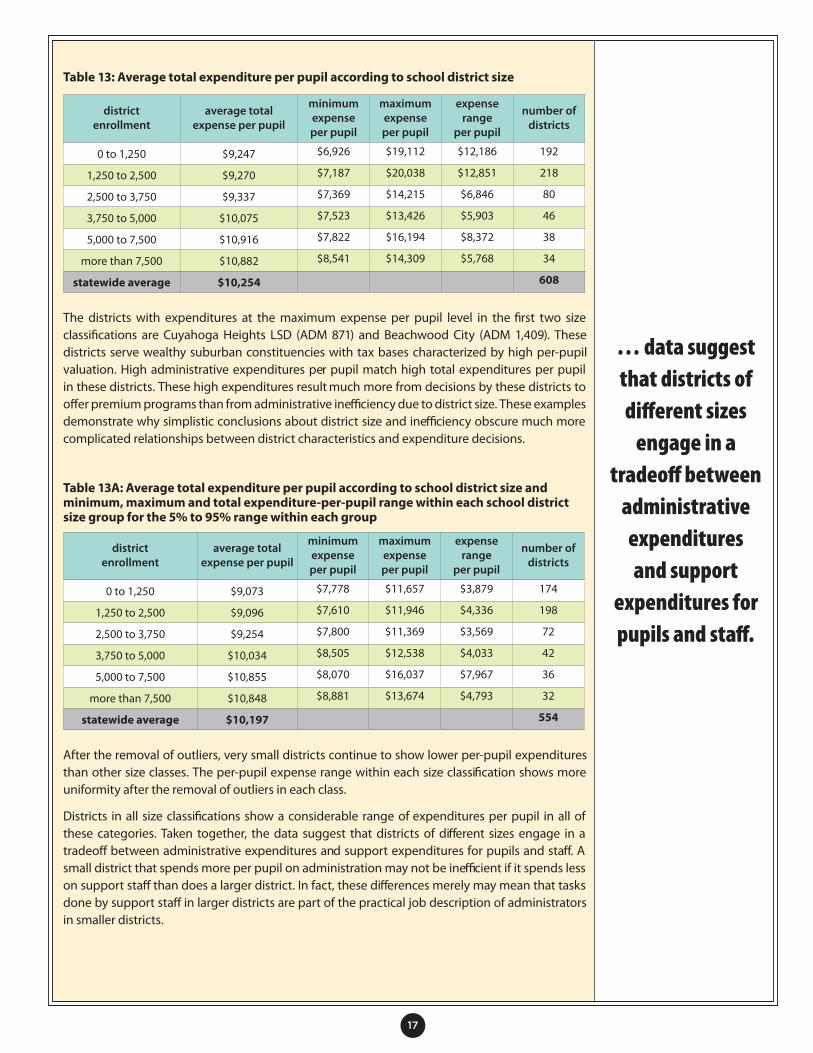
Consideration of total expenditures per pupil shows that smaller districts expend fewer dollars per pupil on average than larger school districts. The smallest class of school dis-tricts, shown in Row 1 on Table 13, spent $1,000 less per pupil than the statewide average. These same districts spent about $500 per pupil less than the average for all districts in the other ! ve size classi! cations.

17

Table 13: Average total expenditure per pupil according to school district size

districtenrollment

average total expense per pupil



expenserange

per pupil

number of districts

0 to 1,250 $9,247 $6,926 $19,112 $12,186 192

1,250 to 2,500 $9,270 $7,187 $20,038 $12,851 218

2,500 to 3,750 $9,337 $7,369 $14,215 $6,846 80

3,750 to 5,000 $10,075 $7,523 $13,426 $5,903 46

5,000 to 7,500 $10,916 $7,822 $16,194 $8,372 38

more than 7,500 $10,882 $8,541 $14,309 $5,768 34


The districts with expenditures at the maximum expense per pupil level in the ! rst two size classi! cations are Cuyahoga Heights LSD (ADM 871) and Beachwood City (ADM 1,409). These districts serve wealthy suburban constituencies with tax bases characterized by high per-pupil valuation. High administrative expenditures per pupil match high total expenditures per pupil in these districts. These high expenditures result much more from decisions by these districts to o# er premium programs than from administrative ine" ciency due to district size. These examples demonstrate why simplistic conclusions about district size and ine" ciency obscure much more complicated relationships between district characteristics and expenditure decisions.

Table 13A: Average total expenditure per pupil according to school district size and minimum, maximum and total expenditure-per-pupil range within each school district size group for the 5% to 95% range within each group

districtenrollment

average total expense per pupil



expenserange

per pupil

number of districts

0 to 1,250 $9,073 $7,778 $11,657 $3,879 174

1,250 to 2,500 $9,096 $7,610 $11,946 $4,336 198

2,500 to 3,750 $9,254 $7,800 $11,369 $3,569 72

3,750 to 5,000 $10,034 $8,505 $12,538 $4,033 42

5,000 to 7,500 $10,855 $8,070 $16,037 $7,967 36

more than 7,500 $10,848 $8,881 $13,674 $4,793 32


After the removal of outliers, very small districts continue to show lower per-pupil expenditures than other size classes. The per-pupil expense range within each size classi! cation shows more uniformity after the removal of outliers in each class.

Districts in all size classi! cations show a considerable range of expenditures per pupil in all of these categories. Taken together, the data suggest that districts of di# erent sizes engage in a tradeo# between administrative expenditures and support expenditures for pupils and sta# . A small district that spends more per pupil on administration may not be ine" cient if it spends less on support sta# than does a larger district. In fact, these di# erences merely may mean that tasks done by support sta# in larger districts are part of the practical job description of administrators in smaller districts.

… data suggest that districts of di" erent sizes

engage in a tradeo" between

administrative expenditures and support

expenditures for pupils and sta" .

18

C. Other measures

While the smallest districts tend to spend less in total expenditures per pupil, they do not necessarily provide inferior services. Table 14 shows the average ratio of pupils to teachers in school districts ranked according to size.

The table shows that the pupil-teacher ratio tends to increase with district size. The smallest classi! cation of school districts has one fewer pupil per teacher than the next best classi! cation in Row 2. These very small districts have two fewer pupils per teacher than the school districts recorded in Rows 4 and 6.

Table 14: Average ratio of pupils to teachers according to school district size

district enrollment pupil-to-teacher ratio

0 to 1,250 16.84

1,250 to 2,500 18.30

2,500 to 3,750 18.77

3,750 to 5,000 19.00

5,000 to 7,500 18.44

more than 7,500 19.25

statewide average 18.47

Therefore, not only do the smallest districts spend less per pupil than the districts in the other size classi! cations, they also appear to o# er smaller class sizes on average than the larger school districts.

Table 15 provides a di# erent kind of perspective. It shows the average geographical size of school districts measured in square miles relative to school district enrollment size.

Table 15: Average size of school districts in square miles according to enrollment size

districtenrollment

average size in square miles

minimum size insquare miles

maximum size in square miles

size range insquare miles

0 to 1,250 63.25 1 239 238

1,250 to 2,500 80.33 2 416 414

2,500 to 3,750 80.13 4 546 542

3,750 to 5,000 49.15 5 487 482

5,000 to 7,500 31.58 6 140 134

more than 7,500 46.88 16 137 121

statewide average 67.71

The smallest districts average about 63 square miles in size. The next two school district classi! cations based on enrollment size have even greater average geographical size. These two classes of district average about 80 square miles in size. In a district with a simple square shape, this territorial size implies an area de! ned by almost nine miles on a side. The smallest districts would form squares of about eight miles on a side.

It is not possible to ignore the fact that the

geographical size of Ohio relative

to the total number of pupils

constrains the state’s ability to change average

pupil density in every place to maximize

e# ciency.

19

Table 16 provides another perspective related to geographical size of school districts. It shows the pupil density in terms of the number of pupils per square mile of area.

Table 16: Average density of school districts in pupils per square mile according to enrollment size

districtenrollment

average pupildensity

minimumpupil

density

maximumpupil

density

rangein pupil density

0 to 1,250 40 5 574 569

1,250 to 2,500 83 5 1,096 1,091

2,500 to 3,750 117 5 870 865

3,750 to 5,000 218 8 782 774

5,000 to 7,500 319 38 974 936

More than 7,500 354 148 774 625

The smallest districts in terms of enrollment also have a pupil density less than half of the school districts in the next largest classi! cation. The fact that the statewide average density only equals a little more than the density in the smallest districts suggests that no matter how the state combines school districts, some districts must have extremely low density. It is not possible to ignore the fact that the geographical size of Ohio relative to the total number of pupils constrains the state’s ability to change average pupil density in every place to maximize e" ciency. An increase in the size of school districts by enrollment also requires an increase in area. Together, those changes would not necessarily change pupil density. It is possible that low-density student populations receive better service from smaller operational units than they would receive from larger units of greater geographical and enrollment size. It also must be accepted that the ability to structure Ohio’s education delivery system in a way that drives every district to some theoretical ideal of “e" ciency” will be necessarily constrained by issues of geography, location, pupil density and other similar factors.

CONCLUSION

The concept of organizational units in the EBM provides a basis for estimating the size of a “model” school district. Such a district would have about 2,500 pupils. A ranking of school districts based on this principle o# ers an opportunity to assess the relative average e" ciency of school districts in di# erent size classi! cations.

While an initial analysis based on the number of administrators and administrative expenditures seems to suggest that the 192 very small districts tend to show some “ine" ciency” in their operations, expansion of the analysis to include other expenditures tends to show just the opposite. The very small districts deliver their services for fewer dollars per pupil. At the same time, the very small districts average smaller pupil teacher ratios than other school districts.

Furthermore, geographical size and pupil density data show that constraints imposed by the average density of pupils in Ohio constrain the state’s ability to deliver educational services in districts of uniform sizes.

20

Looking aheadIt is recommended that a qualitative analysis be performed with an eye to determining how the culture of small school districts di" er from their larger counterparts. Such a study might examine questions such as:

• Are di" erent skill sets required and used by sta" ?

• What aspects of the small school culture can be adapted to larger districts?

• What e# ciencies and cost-saving strategies can be incorporated into small school district operations?

• How can one preserve the advantages of small size while reducing those cost disadvantages that may exist?

As policymakers examine and consider school district consolidation as a potential means to reduce overall costs, such consideration must be with full knowledge and understanding of both the positive and negative associated factors.

21

APPENDIX 1: EMIS STAFF DATA ADMINISTRATIVE POSITION CATEGORIES

Position DescriptionCode

101 Administrative assistant assignment An assignment to perform activities assisting an executive o" cer in performing

assigned activities in the school district.

103 Assistant, deputy/associate superintendent assignment An assignment to a sta# member (e.g., an assistant, deputy or associate

superintendent or the assistant) to perform high-level, system-wide executive management functions in a school district.

104 Assistant principal assignment An assignment to a sta# member (e.g., an assistant, deputy or associate principal) to

perform high-level executive management functions in an individual school, group of schools or unit(s) of a school district.

108 Principal assignment An assignment to a sta# member to perform highest-level executive management

functions in an individual school, groups of schools or unit(s) of a school district.

109 Superintendent assignment An assignment to a sta# member (e.g., chief executive of schools or chancellor) to

perform the highest-level, system-wide executive management functions of a school district.

110 Supervisor/manager assignment An assignment to oversee and manage sta# members, but not to direct a program or

function. If this is a certi! cated/licensed position, an individual hired as a supervisor/manager is required to hold a supervisor certi! cate. NOTE: A supervisor/manager is di# erent from a director, in that a supervisor/manager manages sta# members, but does not direct a program, function or supporting service.

112 Treasurer assignment An assignment to a sta# member (appointed directly by the board of education)

to act as secretary to the board of education, serve as the chief ! scal o" cer and to perform high level, system-wide executive management functions of a school district.

113 Coordinator assignment An assignment to a sta# member to oversee one or more programs or projects. This

is a sta# position, not a line position.

114 Education administrative specialist assignment An assignment to a sta# member to perform highest-level executive management

functions in a central o" ce position relative to business management, education of exceptional children, educational research, educational sta# personnel administration, instruction services, pupil personnel administration, school-community relations or vocational directorship.

22

115 Director assignment An assignment to direct sta# members and manage a function, a program or a

supporting service. Sta# members having this position include heads of academic departments and directors and managers of psychological services. If this is a certi! cated/licensed position, an individual hired as a director is required to hold a director, superintendent or principal certi! cate.

116 Community school administrator assignment An assignment to a sta# member (e.g., chief executive of schools or chancellor)

to perform the highest-level, system-wide executive management functions of a community school.

120 ESC supervisor assignment An assignment to a position to provide supervisory services to ESC member

districts (as provided by ORC §3313.843) that is funded by supervisory units per ORC §3317.032.

199 Other o# cial/administrative assignment Any assignment not listed above that ful! lls the de! nition of the o" cial/

administrative classi! cation.

Source: Ohio Department of Education EMIS Manual 2010

Note: When school districts or ODE count administrators, compute pupil-to-administrator ratios, or estimate administrative expenditures, these positions and the salaries paid to the people who hold them should provide the underlying data. However, we do not know whether the information in the Cupp Report relies only on these data to estimate administrative functions and costs. We do not know to what extent data are reported correctly.

For additional information about position descriptions for non-administration assignments in school districts, refer to the 2009 and later ODE EMIS Manual Appendix D Position Codes.

23

APPENDIX 2: ODE TYPOLOGY DEFINITIONS

1 Rural/agricultural — high-poverty, low-median income - These districts are rural agricultural districts and tend to be located in the Appalachian area of Ohio. As a group they have higher-than-average poverty, the lowest average median income level and the lowest percent of population with a college degree or higher compared to all of the groups. N=96, Approximate total ADM=160,000.

2 Rural/agricultural — small student population, low poverty, low-to-moderate median income - These tend to be small, very rural districts outside of Appalachia. They have an adult population that is similar to districts in Group 1 in terms of education level, but their median income level is higher and their poverty rates are much lower. N=161, Approximate total ADM=220,000.

3 Rural/small town — moderate-to-high median income - These districts tend to be small towns located in rural areas of the state outside of Appalachia. The districts tend to have median income levels similar to Group 6 suburban districts, but with lower rates of both college attendance and managerial/professional occupations among adults. Their poverty percentage is also below average. N=81, Approximate total ADM=130,000.

4 Urban — low median income, high poverty - This category includes urban (i.e. high population density) districts that encompass small or medium size towns and cities. They are characterized by low median incomes and very high poverty rates. N=102, Approximate total ADM=290,000.

5 Major urban — very high poverty - This group of districts includes all of the six largest core cities and other urban districts that encompass major cities. Population densities are very high. The districts all have very high poverty rates and typically have a very high percentage of minority students. N=15, Approximate total ADM=360,000.

6 Urban/suburban — high median income - These districts typically surround major urban centers. While their poverty levels range from low to above average, they are more generally characterized as communities with high median incomes and high percentages of college completers and professional/administrative workforce. N=107, Approximate total ADM=420,000.

7 Urban/suburban — very high median income, very low poverty - These districts also surround major urban centers. They are distinguished by very high income levels and almost no poverty. A very high percentage of the adult population has a college degree, and a similarly high percentage works in professional/administrative occupations. N=46, Approximate total ADM=240,000.

Source: Ohio Department of Education

24

REFERENCES

Cotton, K. (1999) “School Size, School Climate and Student Performance.” School Improvement Research Series. Northwest Regional Educational Laboratory, Portland, OR.

Darden, E.C. (2005) “The Power of Sharing.” Leadership Insider. National School Boards Association, Alexandria, VA.

Duncombe, W. and Yinger, J. (2001) “Does School District Consolidation Cut Costs?”Center for Policy Research, Syracuse University, Syracuse, NY.

Duncombe, W. and Yinger, J. (2010) “School District Consolidation: The Bene! ts and Costs.” The School Administrator, May 2010, pp. 10-18.

Howley, C. (1994) “The academic e# ectiveness of small-scale schooling.” ERIC Digest, ERIC Clearinghouse on Rural Education and Small Schools, Charleston, WV.

National Center for Educational Statistics (2009) “Digest of Educational Statistics.” US Department of Education, Washington, DC.

Pennsylvania School Boards Association (2009) “Merger/Consolidation of School Districts — Does it Save Money and Improve Student Achievement?” Harrisburg, Pa.

Raywid, M.K (1999) “Current Literature on Small Schools,” ERIC Clearinghouse on Rural Education and Small Schools, Charleston, WV.

Wenders, J.T. (2003) “Consolidation is a bad idea.” The Education Gad$ y, Thomas B. Fordham Institute, Dayton, OH.

Yocum, R. (Ed) (2007). “Ohio Schools — Does Size Matter?” OPEC Update. Ohio Public Expenditure Council, Columbus, OH.

AUTHORS

Damon Asbury, director of legislative services, Ohio School Boards Association William P. Driscoll, lawyer and partner, Fleeter & DriscollDr. Howard B. Fleeter, partner, Fleeter & DriscollMichelle Francis, lobbyist, Ohio School Boards Association

Ohio School Boards Association8050 N. High Street

Suite 100Columbus, Ohio 43235-6481

(614) 540-4000(800) 589-OSBA

www.ohioschoolboards.org

school · pdf filean analysis of public school expenditures in ohio reveals that ... center,...

Documents