scf0104 farmscoperextension report 8 - gov.uk
TRANSCRIPT

1
Farmscoper Extension
Defra Project SCF0104
Gooday, RD., Anthony, SG., Durrant, C., Harris, D., Lee, D., Metcalfe, P.,
Newell-Price, P., Turner, A.
October 2015
ADAS UK Ltd

2
Executive Summary
Farmscoper is a decision support tool that allows the assessment of the cost and effectiveness of
mitigation methods against multiple pollutants and multiple targets. This approach is designed to
allow a more holistic assessment of the mitigation of diffuse agricultural production given the
different policy targets (e.g. Water Framework Directive, Climate Change Act, and the Gothenburg
Protocol) and identify the mitigation methods that provide multiple benefits. Under this project, the
scope of Farmscoper has been widened. In addition to the existing capability to model nitrate,
phosphorus, sediment, ammonia, methane, nitrous oxide, plant protection products and biodiversity,
the tool now also calculates baseline values and the impacts of mitigation implementation for faecal
indicator organisms (FIOs), energy use, soil carbon stocks and agricultural production. This not only
increases the pollutant coverage of Farmscoper (and thus its applicability to other policy areas, e.g.
the Bathing Water Directive), but the explicit calculation of production allows for the identification of
mitigation methods that can help to achieve target pollutant reductions whilst not reducing food
production.
Farmscoper relies on a pre-populated database of smart export coefficients, so that models do not
need to be run in real time when Farmscoper is being used. The coefficients for FIO emissions were
calculated by creating a meta-model of an existing ADAS farm scale FIO model, and then applying this
model to the whole of England and Wales and then summarising the values by the soil and climate
zones used within Farmscoper. This approach is designed to ensure that the results of Farmscoper
scale with the area modelled, such that they should reproduce the national totals if Farmscoper is
applied to the whole of England and Wales. Coefficients for emissions of carbon from energy use are
specified for a number of field operations (which the user can select for each crop type), as well as
other livestock and crop management decisions. For each of these operations and management
practices, the energy use has been assessed using a selection of models, literature and machine
performance standards. Calculations of soil carbon stocks are based upon an enhanced IPCC tier 1
methodology taking into account the findings of recent Defra-funded work. Agricultural production is
specified as the monetary output of the various crops and livestock types found on the farm. The unit
values for the output prices are taken from the new Cost Workbook (see below), to ensure
consistency between prices used for the calculation of production and those used in the assessment
of cost of mitigation implementation.
Farmscoper contains default rates for mitigation method implementation, reflecting typical current
practice in England and Wales, and which allow for the true impact of any future additional mitigation
method implementation to be calculated. These default values have been thoroughly revised and
updated within this project, using the available national stratified survey data. The stratification
allowed for default rates to be specified which vary by farm type and soil type.
The Farmscoper tool uses cost coefficients, expressed per m3 of livestock excreta or waste, per ha of
arable or grassland or per kg of fertiliser, to determine the farm scale costs of mitigation method
implementation (by multiplying the coefficients by the m3 of livestock excreta etc on the farm being
modelled). This cost data had been collated over a number of years, reflecting different assumptions
and prices for common items from the various source documents, and the only information on the
data was the limited statements available in the Mitigation Method User Guide (Newell-Price et al,
2011). In order to make the cost data within Farmscoper more robust, a new Cost workbook has been
added to Farmscoper suite of workbooks. This Cost workbook contains a list of all the unit cost items
that are needed by the various mitigation methods (e.g. a metre of fencing, a kilogram of nitrogen
fertiliser, a cubic metre of cement, a water trough), together with referenced prices for all these
items, and a list of all farm management assumptions that may be common to multiple methods (e.g.
typical field length, average fertiliser rate). Each mitigation method can then draw from these two
itemised lists, ensuring a common and consistent approach. The tool contains one worksheet for each
mitigation method, stating the farm assumptions and unit costs that are required, along with any
other assumptions that may needed but which are specific to an individual method (e.g. buffer
width). From all this information, the total cost of implementation is derived, along with the cost
coefficients required for Farmscoper. The Cost workbook has been designed to operate as a stand
alone tool, capable of calculating the costs of implementation at farm scale, as well as providing the
cost coefficient data required by Farmscoper to calculate cost and effect of mitigation method

3
implementation. The Cost workbook reports both upfront and amortised capital costs, and annual
fixed, variable and output costs.
The Farmscoper suite of workbooks has been expanded to include a workbook which allows the
Farmscoper tool (originally developed for application at farm scale) to be applied for multiple farms at
catchment to national scale. The tool uses agricultural census data and counts of the number of
different farm types, along with farm and crop type specific data on fertiliser, manure and livestock
management to automatically populate all of the Farmscoper workbooks that would be needed to
represent the farming systems in the different climate and soil zones in a given area. The user can
then assess different mitigation scenarios against some or all of these farming systems. This Upscaling
workbook can also act as an interface to allow easier population and assessment of multiple farms
than simply using multiple copies of the existing Farmscoper workbooks. The Upscaling workbook has
been populated with agricultural census data at a range of spatial scales. Treating England as one
single catchment allows for a very rapid assessment of national scale policy implications. The
workbook also contains census data for the 88 water management catchments (WMC) that cover the
whole of England. This allows for a much more detailed assessment of national policy, or for the user
to investigate the impacts in a more targeted way. The total agricultural emissions for methane and
nitrous oxide, calculated using the Upscaling workbook to model the whole of England, are shown to
be comparable to official IPCC inventory values (2% lower for methane, 11% higher for nitrous oxide),
whilst values for ammonia are almost 20% higher than the UK Ammonia Inventory. Note that these
Farmscoper values are prior to implementation of mitigation, whereas the inventory approaches can
include some mitigation practice. There are also differences in emissions from Farmscoper and the
inventories due to different assumptions made about farm practices, e.g. the proportions of manure
managed as slurry. The values calculated by the Upscaling tool for nitrogen, phosphorus and sediment
emissions at WMCs correlate well with the results from the source models from which the pollutant
emissions coefficients were derived when this is also summarised to WMC level. The ability of the
Upscaling tool to calculate the impacts of mitigation is demonstrated through a theoretical scenario
where all methods in the Farmscoper mitigation method library. This scenario is shown to result in
national reductions of pollutant loads of up to 38%, with methane the smallest reduction at 14%.
There is also a 27% reduction in energy use and an 8% reduction in production. The total cost of
implementation is £1,576m, but the estimated environmental benefit of these reductions is only
£659m (although it should be kept in mind this is a hypothetical demonstration of the tool’s capability
as opposed to a realistic policy scenario).
4
Table of Contents
1 INTRODUCTION .......................................................................................................................... 5
1.1 PROJECT OBJECTIVES ...................................................................................................................... 6
2 DEVELOPMENT OF THE FARMSCOPER COST WORKBOOK ........................................................... 7
3 DEVELOPMENT OF THE FARMSCOPER UPSCALING WORKBOOK ............................................... 11
3.1 AUTOMATED GENERATION OF FARM TYPES TO USE FARMSCOPER CREATE ............................................... 11 3.2 AUTOMATED USE OF MULTIPLE FARMS IN FARMSCOPER EVALUATE ........................................................ 15 3.3 AGRICULTURAL CENSUS DATA INCLUDED WITHIN FARMSCOPER ............................................................. 15
4 EXTENDED COVERAGE OF FARMSCOPER .................................................................................. 18
4.1 FIOS ......................................................................................................................................... 19 4.2 SOIL CARBON .............................................................................................................................. 19 4.3 ENERGY USE ............................................................................................................................... 21 4.4 FARM PRODUCTION...................................................................................................................... 31 4.5 SOIL PHYSICAL QUALITY ................................................................................................................. 31 4.6 ENVIRONMENTAL BENEFIT ............................................................................................................. 32
5 REVIEW OF PRIOR IMPLEMENTATION RATES ........................................................................... 34
5.1 SOIL MANAGEMENT ..................................................................................................................... 41 5.2 MANUFACTURED FERTILISER MANAGEMENT ..................................................................................... 42 5.3 ORGANIC MANURE MANAGEMENT ................................................................................................. 43 5.4 CROP PROTECTION CHEMICAL MANAGEMENT ................................................................................... 45 5.5 LIVESTOCK MANAGEMENT ............................................................................................................ 46 5.6 HOUSING AND YARD MANAGEMENT ............................................................................................... 47 5.7 FIELD CONNECTIVITY MANAGEMENT ............................................................................................... 47 5.8 IRRIGATION MANAGEMENT ........................................................................................................... 50 5.9 BIODIVERSITY MANAGEMENT......................................................................................................... 50 5.10 NITRATE VULNERABLE ZONE ACTION PROGRAMME ............................................................................ 51
6 FARMSCOPER RESULTS ............................................................................................................. 52
6.1 COMPARISON OF COST RESULTS WITH THE PREVIOUS VERSION OF FARMSCOPER ....................................... 52 6.2 COST SENSITIVITY ......................................................................................................................... 54 6.3 FIOS, SOIL CARBON, ENERGY USE AND PRODUCTION ......................................................................... 62 6.4 UPSCALING ................................................................................................................................. 64
7 DISCUSSION AND CONCLUSIONS .............................................................................................. 77
7.1 FUTURE WORK ............................................................................................................................ 79
8 REFERENCES ............................................................................................................................. 81

5
1 Introduction
The policy targets for the reduction of diffuse pollutant losses to air and water vary by pollutant. The
United Kingdom is legally bound to reduce greenhouse gas emissions by 80% by 2050, and to reduce
CO2 emissions by 26% by 2020 (Climate Change Act, 2008). The United Kingdom is also required to
reduce ammonia emissions to 297 kt yr-1 under the Gothenburg Protocol. The Nitrates Directive
(81/676/EEC) sets a standard of 50 mg l-1 NO3 for nitrate concentrations in surface and ground waters.
The UK implementation of the Water Framework Directive (2000/60/EC) sets phosphorus
concentration standards of 50 to 120 ug l-1 for good ecological status, and the Freshwater Fish
Directive (78/659/EC) sets a guideline target of 25 mg l-1 suspended solids for salmonid and cyprinid
waters. Achieving these quality standards will require wide ranging reductions in pollutant loads from
the agricultural sector. However, it is also necessary to ensure the farming industry remains
competitive and sustainable, whilst providing other ecosystem services. Thus there is a need to
investigate the impacts of potential agricultural mitigation methods, in terms of their impacts on the
different agricultural pollutants and the cost of implementing these different methods, allowing
comparison of the relative cost-effectiveness methods with any environmental benefit.
The suitability and appropriateness of different mitigation methods depends upon, among other
things, the farming system and the local physical environment. There has been considerable research
into the impacts of different mitigation methods on agricultural diffuse pollution pressures and these
continue to be synthesised into manuals or dictionaries of best practice. However, whilst providing
useful guidance documents, these manuals do not all cover a similar range of pollutants and
mitigation methods and they also differ in terms of the scales covered (e.g. plot, field, farm or
landscape scale). This past research highlights the importance of providing quantitative results on the
basis of a consistent framework. The limited scope of some previous research on agricultural
pollutant mitigation methods has hindered the extrapolation of method efficacies to environments
other than those in which the work was carried out. The large number of potential mitigation
methods that are appropriate to any given situation means that a computational approach is ideally
required for assessing the potential or expected impacts of different combinations of methods on
multiple pollutants, since the use of models permits the application of a consistent conceptual
framework for the environmental systems under scrutiny.
In light of this, Farmscoper was developed by ADAS under Defra Project WQ0106(3), to allow the
assessment of the cost and effectiveness of mitigation methods against multiple pollutants and
multiple targets. By including an estimation of the cost of implementation, Farmscoper can be used
for assessing the ability for the cost of implementation to be funded by the farming industry itself or
offset by funding or subsidies from the government or other sources. The tool is thus ideal for analysis
of government policy, and is currently the only tool available for such analysis which considers
impacts on multiple pollutants to water, green house gases, air quality and biodiversity. However, for
a robust estimate of the cost-effectiveness, which is imperative if the tool is to be used to provide a
more detailed and realistic estimate of uptake potential (and ability to recognise barriers and
potential methods to address these), then the cost data within the tool needs to be reviewed and
updated, and presented within a format that allows easy subsequent manipulation and examination
of the component costs and assumptions that make up each mitigation method. The Farmscoper tool
operates at the farm scale - this has been cited as one of the tool’s useful features, because it
produces information at the scale which the agricultural community recognise. However, analysis of
government policy, or the assessment of mitigation potential or targeting within a catchment, need to
be performed at a greater scale across a range of farms. Thus there is a need to automate the
generation of multiple farms, based on agricultural census data, which can be used within Farmscoper
for the prediction of pollutant emissions and the assessment of the cost and effectiveness of pollutant
mitigation at range of spatial scales.
To further improve the usefulness of Farmscoper, it is possible to extend the coverage of the model to
encompass more policy areas. Under this project, Farmscoper has been extended to also calculate
baseline pollutant loads and the impacts of mitigation on Faecal Indicator Organisms (FIOs; which are
important for bathing water quality and shellfish production) and carbon dioxide from energy use (to
complement nitrous oxide and methane - the existing GHGs within Farmscoper). The tool has also
been expanded to include soil carbon stocks and to explicitly calculate the impacts of mitigation on

6
production. Although any impacts of mitigation implementation on production form part of the cost
of implementation, having this also explicitly represented allows the tool to help in ‘sustainable
intensification’ of the agricultural industry and ensure that any government policy does not have a
detrimental impact on food production.
1.1 Project objectives
The overall objective of the project is to expand the capability of the Farmscoper tool, in order to
improve its functionality for cost-effective assessments of mitigation method implementation for
policy analysis and for use by other stakeholders involved in catchment management.
The specific objectives of the project were:
1. The development of a ‘Cost Tool’ - a custom spreadsheet that provides explicit information
on the source and breakdown of the cost and savings associated with each of the mitigation
methods in the Farmscoper library, which can be linked to from the ‘Evaluate’ spreadsheet of
Farmscoper.
2. The development of an ‘Upscaling Tool’ - a custom spreadsheet which would:
a. Automate the process of building multiple Farmscoper farms, using agricultural
census data, in order to represent the farming within a catchment
b. Automate the subsequent cost-effectiveness assessment of mitigation methods on
these farms
c. Automate the extraction and collation of the results for these multiple farms.
3. To extend the coverage of the tool to include both an estimate of baseline values and the
potential of the mitigation methods currently included within Farmscoper to alter these
values for the following outputs:
a. Faecal Indicator Organisms (FIOs)
b. Soil carbon
c. Farm energy use
d. Farm production
e. Soil physical quality (qualitative impacts of mitigation methods only, no baseline
values)
4. To review the prior implementation rates of the mitigation methods included within
Farmscoper

7
2 Development of the Farmscoper Cost Workbook
The cost data within the previous versions of Farmscoper were drawn from a range of sources,
including previous Defra funded projects, which has resulted in the cost data not reflecting a
particular year and the final values within Farmscoper containing a range of hidden assumptions. The
intention behind the creation of a new cost workbook was to:
1. Create a list of unit cost data (e.g. metre of fencing, kg of fertiliser), from which each
mitigation method could access the unit cost data they required. All the items in the unit cost
list should be representative of the same year.
2. Lay out all the assumptions used in deriving the costs for each method, and where practical
share the common assumptions (e.g. field size) between the different mitigation methods
3. Create a workbook that could act as a standalone tool, and would provide an estimate of the
uncertainty in the costs for a mitigation method.
2.1.1 Unit cost data
A large range of different unit cost data is required, from costs per kilograms, tonnes or metres to
costs per hour or per hectare or costs for individual items. Much of the information for unit costs was
taken from the Farm Management Pocketbook (e.g. Nix, 2013), for example crop or fertiliser prices.
Other costs (e.g. fencing items and concrete) were sourced directly from a range of suppliers.
Yearly values for unit costs have been provided for the years 2000 to 2013. Where values are
unavailable for intervening years, the tool uses linear interpolation between the nearest points to
obtain a complete time series. Where a time series is still incomplete, the tool extrapolates backwards
or forwards as appropriate from the last available value using an annual percentage change
(effectively a retail price index; RPI). The user is able to select to use the unit costs from a specific
year, or for a 5-year average.
For each of the unit costs, there is a value specified for the potential range in that cost. The range is
designed to reflect variations in costs resulting from: geographical location (both in terms of number
of suppliers and distance required to transport goods); the quality of the goods purchased; the
quantity of goods purchased (due to economies of scale); changes in demand and thus price
throughout the course of the year due to the seasonality of demand; terms of supply (e.g. who pays
for fuel used by contractors) and species, management, external market forces and many other
factors for crop and livestock gross margins.
Unit costs are categorised as fixed, output, variable or capital. A mitigation method may give rise to
costs in more than one category. For capital costs, the tool shows both the total ‘up-front’ cost as well
as the amortised cost (where the cost is spread over a period appropriate to the lifetime of the asset).
Previous estimates have generally used the conventional approaches of amortisation at a range of
rates depending on the investment, for example, 10 or 20 years at a conventional interest rate of 7%.
This may appear strange at the present time with record low interest rates operational over a long
period, but it is uncertain when they will change and to what extent. It is also the case that for
comparison, it is better to be consistent than to introduce uncertainties which make it difficult to see
the reason for differences in cost effectiveness, particularly when the factor is the interest rate on a
theoretical calculation. There is also the matter of the number of years which are conventional
although in reality the capital item may be traded in or scrapped after a different number of years for
a whole range of reasons.
Other methods of calculating annual costs may be to work out a straight-line depreciation by dividing
the capital cost simply by a number of years, or by the lifetime in hours. The former may be
appropriate for some machines or a building, but the latter may be more relevant for many other
machines or tyres where the lifetime is better reflected in hours used rather in years owned and the
alternative may have a significantly different lifetime. However, in both these cases, no account is
taken of capital invested as it is in the case of amortisation.

8
2.1.2 Management Plans
A number of the mitigation methods included within Farmscoper are assumed to require the farmer
to assess manure or nutrient use on the farm, either in terms of identifying high risk areas for the
application or storage of manure or fertiliser, or calculating accurate fertiliser application rates. In the
previous cost estimates for Farmscoper, each individual method could be assigned the cost of this
assessment, thus potentially resulting in double-counting where multiple methods were
implemented. To avoid this obstacle, two management plans have been added to the Cost workbook,
a nutrient management plan and a manure management plan (the nutrient management plan
represents time for estimating nutrient supply from soil and applied manures and calculating crop
fertiliser requirements field by field, whilst the manure management plan represents time for
calculating manure production, producing a field risk map, allocating manure to different fields on the
farm, calculating slurry storage requirements and capacity, planning manure field heap storage sites
and assessing risks at spreading). A mitigation method can be associated with one or neither of these
two plans. When an assessment of mitigation effect is performed with the Farmscoper Evaluate
workbook, the two management plans will be implemented according to the highest implementation
rate of any method associated with that particular plan, thus ensuring there is no double-counting
(and if no methods associated with the management plans are implemented, the costs of the
management plans will not be included at all).
2.1.3 Farm details
The Cost workbook contains a number of farm assumptions on the ‘Farm Details’ worksheet. This
allows each mitigation method to select from a list of common assumptions (e.g. typical field size),
but also for the Cost workbook to produce farm level results, which allow its results to be readily
audited by a user, as well as the cost coefficients required by Farmscoper Evaluate (see Section 2.1.6).
By default, the ‘Farm Details’ worksheet is populated with a typical dairy herd, a typical beef and
sheep herd, a typical poultry farm and a typical pig farm, based on the default farm systems in
Farmscoper Create, along with the largest cropping areas for each crop type from the different
default farm systems. This ensures that the coefficient data passed across to Farmscoper Evaluate are
based on realistic farm level data, with every crop and livestock type included. However, these
numbers can be altered to allow the Cost Workbook to function as a stand alone tool for calculating
the cost of mitigation method implementation on a specific farm system.
2.1.4 Mitigation Methods
The implementation of a pollutant mitigation action may alter farm finances by changing the variable
costs and gross margin of a crop or stock enterprise; by changing the fixed costs or overheads
associated with labour and machinery; or by requiring a capital investment (Withers et al., 2003).
Mitigation actions may give rise to costs in more than one category. When determining the costs for
each mitigation method, the workbook only considers the actual costs to the farmer (and not
payments from agri-environment schemes or other incentives). For each method, a typical or simple
approach for costing up the method has been taken - so as not to be distracted by the fine detail that
would be different for every farm – and only the major implications of each method have been
considered.
For each mitigation method, the Cost workbook contains at least one worksheet, with multiple
worksheets required where a method needs to be costed separately for e.g. grassland and arable or
diary and beef livestock. The worksheet for each mitigation method contains a list of the required
farm assumptions for that method, taken from the ‘farm details’ worksheet, and then a list of other
assumptions. This can be seen in the centre of Figure 2-1, which is an example worksheet for one of
the mitigation methods in Farmscoper – ‘Establishing in-field grass buffer strips on arable land’ needs
to know properties of the arable land, such as field length (‘Farm Assumptions’) and other properties
specific to the mitigation method, such as the number of buffers per field and the buffer width (‘Other
Assumptions’). A value is provided for each of these assumptions, together with the units for that
assumption. The values for the different assumptions are then combined to produce the amounts to
multiply the unit costs by. In this example, field length, buffer width and buffers per field (together
with the number of fields) determine the total area of lost arable production, which is then multiplied
by the typical arable gross margin. Each unit cost states whether it is a capital, fixed, variable or

9
output cost, and these are summed to show the total costs by these categories (including both
upfront and annual amortised value for capital costs), and also the total overall cost.
The Farmscoper Evaluate workbook requires cost coefficients (see Section 2.1.6) for each method,
rather than the total cost, so the worksheet for each mitigation method allows the specification of all
the details to produce these values required. There is also the option to specify whether or not the
mitigation method is associated with either the manure or nutrient management plans.
2.1.5 Sensitivity
Each of the unit cost data items have a range assigned to them (defined as a potential percentage
change in the value) to reflect the uncertainty in the value for that item. The Cost workbook can be
used to assess the sensitivity of the total costs of each mitigation method to this potential range in
the unit costs. For this assessment, a value for each item in the unit cost list is selected between the
minimum and maximum values, and the total cost for a method recorded. Note that the sampling is
not correlated for any cost item, such that one may be near its maximum value whilst another is near
its minimum. This process is repeated 1,000 times, allowing the 95th percentile values for the total
implementation cost for each mitigation method to be identified.
Note that this sensitivity analysis is only designed to function within the Cost workbook as a
standalone tool, and the percentile values are not passed over to the Farmscoper Evaluate workbook.
2.1.6 Cost coefficients
To enable scaling of the costs and application to a range of farm types and sizes, the total annual cost
of implementation is re-expressed as a cost coefficient in one of four ways:
1. Excreta cost coefficient
The annual mitigation action cost is expressed per cubic metre of livestock excreta produced on a
farm. The assumption is that the cost represents farm inputs that are directly in proportion to the
numbers of animals, and hence the total quantity of excreta produced on the farm. For example,
dietary supplements are in proportion to the animal diet and therefore excreta production; and the
roofing of concrete yards will be in proportion to the yard size that is also in proportion to animal
numbers or excreta production. In effect, excreta production is used as a form of livestock unit.
2. Manure cost coefficient
The annual mitigation action cost is expressed per cubic metre of managed slurry or farm yard
manure on a farm. The assumption is that the cost represents additional handling and storage costs
that are in proportion to the quantity of manure. For example, restrictions on the placement of
manure next to watercourses require additional planning time; and restrictions on timing of manure
application may require additional storage facilities.
3. Area cost coefficient
The annual mitigation action cost is expressed per hectare of arable, grass or rough grazing on the
farm. The assumption is that the cost represents income foregone or labour that is in proportion to
the land area. For example, riparian buffer zones require land to be taken out of production; and the
cultivation of compacted soils requires an extra tillage operation.
4. Fertiliser cost coefficient
The annual mitigation action cost is expressed per kg of nitrogen or phosphorus fertiliser applied. The
assumption is that the cost of implementation is directly proportional to the original amount of
fertiliser applied pre-mitigation implementation, for example, replacing urea fertiliser with
ammonium nitrate.
Cost coefficients are provided for capital costs (using the amortised value) and for operational costs
(the sum of the fixed, variable and output costs). These cost coefficients are multiplied within
Farmscoper Evaluate by the appropriate scalar (e.g. m3 of dairy slurry; ha of arable land) as loaded up
from the Farmscoper Create workbook.

10
Figure 2-1 Example page for a mitigation method taken from the Farmscoper Cost workbook
11
3 Development of the Farmscoper Upscaling Workbook
The Farmscoper tool was designed to operate at farm scale. However, a number of users have tried to
apply the model to multiple farms in order to represent a catchment or larger area. This has been
found to be a relatively time consuming and laborious process, and so a new workbook has been
added to Farmscoper to enable the rapid population and assessment of multiple farms.
In summary, the new Farmscoper Upscaling workbook has two principal stages: the first stage
populates a number of Farmscoper Create workbooks, the second stage takes one or more pre-
existing Farmscoper Create workbooks, passes them through a specified copy of Farmscoper Evaluate
and then summarises the results. The user is able to repeat the second stage with different Evaluate
workbooks in order to investigate different mitigation method scenarios. The Upscaling workbook is
able to automate and streamline the use of the Create and Evaluate workbook such that multiple
farm scale simulations can be performed per minute.
The Upscaling workbook has been designed to work with up to 10 different farm types, reflecting the
9 major Robust Farm Types used by Defra, plus an extra slot for Outdoor Pig farming (although the
user can alter these 10 farm type slots if desired). The Upscaling tool effectively has 10 copies of the
data entry section from the ‘Farm’ worksheet from Farmscoper Create. Each of the 10 farm data entry
sections has a space where the count of that farm type occurring on each of the climate and soil types
recognised by Farmscoper can be entered. At its simplest, the user can directly enter the farm details
(crop areas, livestock types, manure management etc) and farm counts by soil / climate, and then
automate the production of a Farmscoper Create workbook for each farm, soil and climate type
combination. However, the more expected use of the tool is to automate the generation of the farm
details from census and survey data, and this process is discussed below.
3.1 Automated generation of farm types to use Farmscoper Create
The automated generation of farm types is based upon a number of datasets which are included
within the Upscaling tool and are editable by the user. The datasets, and how they are used, are
described below.
3.1.1 Farm counts
For the 10 farm types considered, Farmscoper requires a count of the number of each farm type
found on the different soil and climate types available within Farmscoper. If prior implementation
rates are going to be specified and vary according to whether farms are inside or outside NVZs, then
the farm count by soil and climate type will also need to be stratified by inside / outside NVZ.
For the default data included within the Upscaling tool, the location of each RFT recorded as part of
the 2010 June Agricultural Census was integrated with a spatial dataset containing the climate and
soil zones recognised by Farmscoper, along with the 2013 NVZ boundary, in order to determine the
farm count data required by the tool.
3.1.2 Census data
For each area considered, Farmscoper needs to know the livestock and cropping within that area,
totalled according to the livestock and crop categories recognised by Farmscoper.
The default data included within the Upscaling tool is taken from the 2010 June Agricultural Census,
with census categories modified to fit the Farmscoper categories.
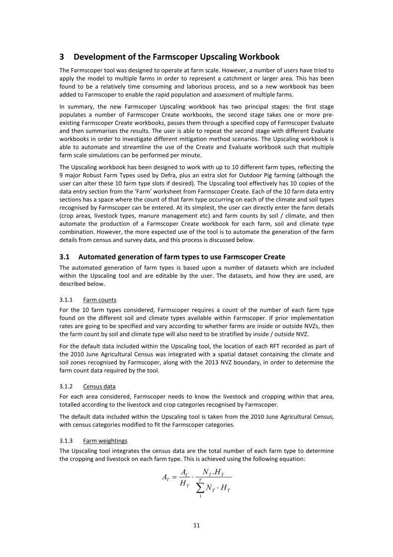
3.1.3 Farm weightings
The Upscaling tool integrates the census data are the total number of each farm type to determine
the cropping and livestock on each farm type. This is achieved using the following equation:
∑ ⋅
⋅=T
TT
TT
T
C
T
HN
HN
H
AA
1
.

12
where AT is area of a crop type or number of livestock on farm type T within the catchment, AC is the
total area of a crop type or number of livestock in the catchment, NT is the typical crop area or
livestock count on farm type T and HT is count of farm type T in the catchment. Farmscoper contains
typical data for crop areas and livestock counts based upon the representative farm systems included
in the previous and current versions of Farmscoper Create. A subset of these weightings is shown in
Figure 3-1.
As an example of this weighting based approach, consider a catchment with 400 “Dairy Cows and
Heifers”, 2 dairy farms and 3 mixed livestock farms. The weightings in Figure 3-1 show that there are
110 “Dairy Cows and Heifers” on a typical dairy farm, but only 31 on a mixed farm; using the equation
above results in the 2 dairy farms in this catchment having 140 cows each and the mixed farms having
40 cows each (thus maintaining the livestock ratio of 3.5 between the two farm types).
Note that the weightings do not need to be expressed in terms of typical numbers, as it is actually the
relativity between the numbers on different farms that is important. However, it is felt that using
typical farms makes the weightings easier to visualise.
The use of the weightings in isolation may result in over or under-stocking of various farm types. The
weightings are modified within the tool on an iterative basis until any specified criteria for minimum
and maximum stocking densities (expressed in terms of kg excretal N per hectare) are achieved.
Figure 3-1 shows that the default set up is for no farm to be stocked at over 170 kg N ha-1
(approximating the stocking limits as specified by the NVZ Action Programme), with some farms
having a minimum stocking density of 130 kg N ha-1 (reflecting the fact that they are typically the
more intensively stocked farms). The other item of information in Figure 3-1 shows how the
weightings are to be modified in order to try and achieve these constraints – either by lowering the
livestock weightings (Density D) or altering the area (Area U/D). The Upscaling tool first calculates the
cropping and livestock by farm type using the initial weightings. Then it assesses the stocking densities
for each farm type against the stocking density criteria and, if needed, calculates an appropriate
modifier, which is then applied to all of the livestock weightings or all of the crop weightings for that
specific farm type. The tool then recalculates the cropping and livestock by farm type using the
modified weightings, before then assessing them again against the criteria. This process is repeated
iteratively a number of times until the criteria are reached (note that in a particularly over or
understocked catchments, the tool will not necessarily achieve the specified criteria).
This approach assumes that livestock and cropping do not vary by climate and soil type for a specific
farm type in a catchment. The smaller the catchment (and thus more homogenous the soils and
climate within that catchment), the more realistic the assumption becomes. A more refined approach
would require a more detailed assessment of the input census data (i.e. the census data would need
to be disaggregated by soil and climate as well), which it was felt would dramatically over complicate
the input format and requirements of the tool. However, a user could get around this assumption by
setting the input data up for a series of new ‘catchments’ such that each new catchment contained
only the census data and farm counts for a soil and/or climate type within the original master
catchment.

13
Figure 3-1 Weightings and stocking density targets for some farm types and a number of crop and livestock categories.

14
3.1.4 Fertiliser and pesticide data
The Upscaling tool allows for nitrogen and phosphorus fertiliser rates to be specified by farm type, for
the different crop types recognised by Farmscoper. Default values are provided in the tool based
upon the British Survey of Fertiliser Practice 2010 (BSFP, 2010).
The calculation of losses of pesticides in Farmscoper, as described in previous Farmscoper reports,
was based upon typical fertiliser usage statistics. As per the farm data entry in the Farmscoper Create
workbook, the user is able to specify pesticide usage, by crop, relative to ‘typical practice’. By default,
rates are assumed to be 100% of typical practice for all crops on all farm types.
3.1.5 Manure data
The Upscaling tool uses a weighting-based system to determine the destination of managed manure
on farm. Note that in the Upscaling tool, all manure generated on a farm must also be applied on the
farm and there is no manure import or export – this is why pig and poultry farms often end up being
larger than in real life, as the land receiving the manure, which is typically on other nearby farms, is
instead allocated to the pig or poultry farm thus ensure stocking densities and manure loadings are
not too high.
The manure weights are specified by manure type and by crop type (Figure 3-2). This specifies the
initial ratio of the different manure types applied per ha to the different crop types. If a farm had 200
tonnes of cattle slurry, 20 ha of permanent pasture and 5 ha of winter wheat, the initial allocation to
pasture would be 195 tonnes (200 * (20 * 10) / (20 * 10 + 5 * 1)) and the other 5 tonnes to the wheat
crop. However, this would result in the rate to the wheat crop being less than a realistic minimum
rate (set at 5 tonnes per hectare), so the weighting for the wheat would be ignored in this case and all
manure would be applied to the permanent pasture. An iterative approach is used, with weightings
being adjusted as required on each iteration such that final manure rates are not higher than 250 kg
total manure N per hectare if possible (the 250 value has been selected due to its use within the NVZ
action programme as a field limit for manure applications).
The values in the default manure weightings table (Figure 3-2) have been selected to produce manure
rates that approximate typical national values (for example as found in the representative farm
systems in Farmscoper Create and from literature such as the BFSP (2010). The majority of pig and
poultry manure would be applied to arable crops according to this table, except where there were
significant areas of grassland in a catchment, or where there was too much manure to spread it to
arable crops alone and stay below the field limit.
Figure 3-2 Manure weighting table

15
3.1.6 Production and presentation of results
For a given catchment, the Upscaling tool creates the input data required by Farmscoper Create for
each of the up to 10 farm types. It then populates a copy of Farmscoper Create with this data one
farm at a time, altering just the soil and climate data so that all permutations for that farm type in
that catchment are accounted for, saving a copy of Farmscoper Create (for each farm, soil and climate
type) as it proceeds, before moving on to the next catchment. The Upscaling tool also produces a list
of all of the Farmscoper Create files that have been created, along with the catchment name and the
number of those farms in the catchment.
After building each catchment, farm, soil, climate type combination in Farmscoper Create, the
Upscaling tool records the total pollutant losses (total values and values per hectare), and produces
an area weighted value across the whole set of catchments. This summary data can be copied in to a
separate copy of Excel (or similar software package) for further analysis. It also produces some
graphical output to demonstrate the relative pollutant loss and apportionment by catchment, farm,
soil and climate type.
Note that the copies of Farmscoper Create as saved by the Upscaling tool have a number of
worksheets deleted to reduce the size of each file. This means that although each file can be opened
and its results examined, it cannot subsequently be used as a normal Farmscoper Create file. (i.e. it
would not be possible to open up a file and subtly tweak the setup for one farm, climate and soil type
combination).
3.2 Automated use of multiple farms in Farmscoper Evaluate
The Upscaling tool is able to process one or more Farmscoper Create files through a copy of
Farmscoper Evaluate, thus automating the evaluation of a set of mitigation methods against one or
more farm types.
When the Upscaling tool builds the all farms required to represent one or more catchments, it also
creates a file containing the details of the saved files, number of those farm, soil, climate
combinations etc. When assessing the impacts of mitigation methods, the Upscaling tool looks at the
contents of this file and processes all of the files listed within it through a single copy of Farmscoper
Evaluate. The contents of this summary file can be edited such that the assessment of mitigation
methods is only performed on a subset of all the farm combinations created. The copy of Farmscoper
Evaluate to be used can be set exactly as normal, with a list of active methods, prior and maximum
implementation rates etc. Note that if the default prior implementation rates are selected, these are
adjusted to account for farm type, soil type etc. as accounted for in the default rates. Multiple
assessments can be done, allowing for the impacts of different sets of mitigation methods to be
evaluated against the same set of baseline farm results for a catchment or catchments.
The Upscaling tool saves a copy of each Farmscoper Evaluate file after assessing a farm set up,
allowing the results to be looked at in detail. However, the headline figures (total values and
percentage changes) are also summarised in the Upscaling tool, along with an overall total for all
catchment(s) considered in that assessment. Because these headline results may be all that is
required, there is an option not to save the individual Farmscoper Evaluate files. The Upscaling tool
processes the headline figures to allow a quick assessment of how the pollutant reductions achieved
vary by catchment, farm, soil and climate type. This summary data can also be copied in to a separate
copy of Excel (or similar software package) for further analysis.
Note that both the cost assumptions made within the Cost workbook, and the unit costs values within
it, may become less appropriate as the Upscaling tool is applied to larger areas due to the impacts of
supply and demand.
3.3 Agricultural census data included within Farmscoper
The Farmscoper Upscaling workbook contains agricultural census data for England summarised at
three different spatial scales: the whole of England, by River Basin District (RBD) and by Water
Management Catchment (WMC). The boundaries for RBDs and WMCs are shown in Figure 3-3 and
Figure 3-4 respectively. Note that the tool only contains the data for England, and thus, for example,
only contains part of the data for the Severn RBD and no data for Western Wales RBD.

16
For England, the RBDs and the WMCs, the tool contains the agricultural census for each area,
aggregated according to the Farmscoper crop and livestock categories. The tool also contains data on
the number of farm types within each area in the different soil and climate zones, stratified by inside
or outside NVZs. For the purposes of generating this dataset, the registered address for each farm
holding was assumed to be representative of the location of the farm. To avoid the data within the
tool being disclosive, the total farm count for each farm type was adjusted such that the total farm
count was set to zero if the farm count was 1 or 2 and set to 5 if the farm count was 3 or 4. Note that
the cropping and livestock numbers are not adjusted, so there will be negligible impacts on the
pollutant predictions, just minor changes to the apportionment of pollution by farm type. The total
farm count is 101,699 for England. The disclosure modifications result in 101,706 farms in all the RBDs
and 101,708 farms in total across the WMCs.
The England and RBD level data assumes that 30% of specialist pig farms are outdoor pig farms, with
the remaining 70% being indoors. As there are only 1,600 pig farms in England, at WMC level this split
results in a lot of catchments hitting the disclosure threshold, and so all pig farms are assumed to be
indoor ones for this dataset (also, the assumption that 30% of pig farms are outdoors would be
incorrect for many WMCs).
Figure 3-3 River Basin District boundaries for England and Wales

17
Figure 3-4 Water Management Catchment boundaries for England and Wales

18
4 Extended coverage of Farmscoper
Farmscoper has been expanded to calculate baseline values and impacts of mitigation on faecal
indicator organism (FIO) losses, soil carbon stocks, production and energy use as well as estimating
the impacts of mitigation on soil quality. Farmscoper also now places a financial value on the
environmental benefit of the pollutant reductions.
The optimisation routine with Farmscoper was designed to maximise reductions in the baseline
pollutant emissions. Therefore only FIOs have been added to the list of pollutants that can be
optimised. Although it is likely that users would also want to reduce energy use, it was decided this
was a secondary consequence of mitigation method selection, and thus should not be selectable for
optimisation.
In order to accommodate the new pollutants and outcomes within Farmscoper, it was necessary to
expand the coordinate system used for the source apportionment (Table 4-1). For all pollutants, a
value is taken from each column to give the full apportionment, but for the new outcomes not all
columns are used (i.e. energy use only utilises Source, Area, Type and Form; production only utilises
Source and Type; Soil Carbon only utilises Area and Type).
Table 4-1 The expanded coordinate system used within Farmscoper to accommodate new
pollutants and outputs. New coordinates are italicized.
Source Area Pathway Type Timescale Form
Dairy Arable Runoff Soil Short Particulate
Beef Grass Preferential Fertiliser Medium Dissolved
Sheep Rough Leaching FYM Long Gas
Pigs Yards Gaseous Slurry Gas Indirect
Poultry Housing Direct Litter Gas Embedded
Chemical Tracks Voided
Land Fords Enteric
Arable Products Field Storage Dirty Water
Grass Products Steading Storage PPPs
Woodland Biomass
Boundary Cultivation
Planting
Irrigation
Harvesting
Cleaning
Feeding
Housing
Milking
Output
Internal

19
4.1 FIOs
4.1.1 Calculation of pollutant losses
The calculations of FIO losses were based upon the FIO-Farm model (Anthony and Morrow, 2011).
FIO-Farm is a farm-scale source apportionment tool that determines annual losses of FIOs and
includes explicit representation of the uncertainty in the model parameters such as the microbial die-
off rate. A significant part of the FIO-Farm model determines the potential FIO burden in different
source areas, which has already been taken account of in this work through the farm workbooks.
Meta-models were derived from the sub-models within FIO-Farm in order to derive the proportions of
the potential burdens lost in the different source areas.
For the field losses of FIOs from both excreta and managed manure, the FIO-Farm results for all soil
series in England and Wales were used to determine a HOST class based relationship, which was a
function of annual average rainfall, land use and season of application (whether or not soils were at
field capacity). To capture the impacts of the monthly inputs to the FIO-Farm meta-model, it was
necessary to determine the proportion of each month, D, at which soils were close to field capacity
(defined as within 5mm). This was described statistically by a generalised Michaelis-Menten function
(Lopez et al., 2000) as:
S
S
R
VL
R
VL
D
−+
−
=
'1
' Eq. 4-1
where L is the annual average rainfall (mm), V is a response lag (mm), S is a shape parameter, and R’
(mm) is an effective rate parameter. Values for V, S and R had been derived by Gooday et al (2014) by
fitting this relationship to MORECS data for Scotland (Hough and Jones, 1997), which provided the
proportion of each month at field capacity for each MORECS square, based upon data for 1961-2000.
The calculation of FIO losses was coupled to the PSYCHIC model (Davison et al., 2008) used to
calculate the phosphorus and sediment losses in Farmscoper so that the FIO loss by month could be
apportioned between surface and drain flow according to the relative flow in the two pathways as
determined by the water balance model within PSYCHIC.
Losses of FIOs from excreta on hard standings (yards and farm tracks) were a function of annual
rainfall. Different relationships were derived from FIO-Farm to represent daily cleaning of the yards
(for dairy animals), weekly cleaning of the yard (for beef and sheep animals) and no cleaning (for all
farm tracks). The relationships were average values from the full range of uncertainty in microbial half
lives and wash out factors within FIO-Farm. Based on the data analysed for FIO-Farm, the loss of FIOs
from field heaps was set to 1% of the initial FIO burden within the heap.
4.1.2 Calculation of mitigation method impacts
For the majority of field management options, their impact on FIOs could be inferred from the
impacts on phosphorus and sediment (e.g. a method resulting in a 25% reduction in losses of
phosphorus from manure in surface runoff would be expected to result in a similar 25% reduction in
losses of FIOs in surface runoff from manure spreading). The main exceptions to this relate to manure
storage, where calculations were made based upon faecal die-off. For example, dairy slurry will be
stored at ambient air temperature of c. 5 °C during the winter months, giving an effective half-life
between 6 and 31 days (Anthony and Morrow, 2011), which can be integrated with current and
expected storage durations to determine the consequence of longer manure storage duration.
4.2 Soil carbon
The soil carbon approach uses an enhanced IPCC tier 1 methodology (Eggleston et al, 2006), taking
into account the findings of Defra project SP1113. A stock approach has been used, where the total
carbon stock (t ha-1) is calculated assuming that the land is in equilibrium (both for the baseline
situation and any mitigation scenario). If desired, a rate of change can thus be found by differencing
the baseline and a mitigation scenario and estimating the length of time required to reach the new

20
equilibrium under the mitigation scenario (values typically used are between 20 and 100 years).
Following Defra Project SP1113, the carbon stock was calculated for a depth of 100 cm, although
many of the management factors (see below) were only applied to the top 30 cm.
The carbon stock is calculated for six different areas or features, and also modified to account for soil
erosion, as described below.
4.2.1 Grass
The soil carbon stock of grassland was designed to use the IPCC approach, using default stock change
factors, but Defra project SP1113 concluded that this approach was not reliable for UK grasslands,
largely due to difficulties in defining improved grassland and carbon stocks under rotational grass and
because the stock change factors for grassland management were not appropriate for UK conditions.
However, it was not able to suggest alternative values to be used. Therefore all management factors
for grassland have been set to 1, although the functionality remains embedded within the tool to
modify these. The starting default soil carbon stock to 1 metre for grassland is 130 t ha-1 (Bradley et
al., 2005).
4.2.2 Rough grazing
Rough grazing land has the same default carbon stock as grassland. The land is assumed to be 50%
native and 50% moderately degraded (default stock value * 0.95). Note that in Farmscoper rough
grazing land cannot receive manure or fertiliser, so cannot be receive the improved or high input
factors).
4.2.3 Arable
The default carbon stock value for arable land is 120 t ha-1 (Bradley et al., 2005). The management
factors used depend upon whether the land is low input (0.92), medium input (1.0), high input (1.11)
or high input with manure (1.44). The IPCC approach also has management factors for reduced and
minimum tillage (which increase soil carbon stocks), but SP1113 suggested that these increases in
carbon stock following a reduction in tillage were not appropriate for UK conditions, and as most
arable land is ploughed periodically all UK arable land should be considered to be conventionally
tilled. Consequently tillage was not included as a management factor. A decision tree approach taken
from SP1113 is used to classify the management factor appropriate for each crop type, which
accounts for whether the crop is classified as low residue, if the residues are removed, if manure is
applied to the crop and if fertiliser is applied. The residue classes were taken from SP1113, and typical
practice as to residue removal by crop type was taken from national surveys and, where necessary,
expert judgement. Note that in the arable land calculation there is no minimum threshold value for a
crop to be considered as receiving fertiliser or manure, so even a very low application rate will result
in the higher management factor being applied.
In the IPCC approach there is the potential for a further class of carbon enhancing management.
However, SP1113 concluded this was not currently relevant or quantifiable in the UK landscape.
4.2.4 Wooded Areas
The woodland carbon stock is calculated as a sum of the above ground biomass carbon stock and the
soil carbon stock. The typical woodland above ground biomass is taken from the IPCC default values
(78 t ha-1), with 48% of this considered to be carbon. The soil carbon stock is a fixed value at 170 t ha-1
(Bradley et al., 2005). The carbon stock of wood litter or root biomass is not considered in this tier 1
approach.
4.2.5 Organic Soils
Following the IPCC approach, organic soils are treated separately in the carbon calculations, with a
fixed carbon stock rather than applying crop or grassland management factors to the land use specific
carbon stock. The organic soil carbon stock is 250 t ha-1. There are a number of different ways that can
be used to define organic soils (e.g. Anthony et al, 2013). In Farmscoper, the soil selected for the
calculation of pollutant losses (free-draining, or requiring assisted drainage) is not linked to the
percentage of organic soils. The percentage of organic soils is assumed to be spread equally across the
different land uses.

21
4.2.6 Linear Features
Linear features (field boundaries) are not explicitly considered in the IPCC approach, but can be a
source of carbon stocks where hedges are used. They are considered in Farmscoper in order to
represent the effects of mitigation measures which impact on the extent and type of field boundaries.
Using a typical average field size by land use, an average boundary width, the proportion of
boundaries which are hedgerows and the proportion of boundaries are assumed to belong to the
farm in question (rather than a neighbouring farm, where boundaries are shared), Farmscoper
calculates an assumed area of land that is hedged. This land is given a carbon stock value to represent
the hedge biomass (the contribution of hedges to soil C stocks are not considered, as the area in
question is small and typically included within the stated field areas). The carbon stock of a hedge can
be highly variable depending on structure and has not been well studied in the UK. Farmscoper uses
the figure of 5 t ha-1 from Falloon et al. (2004).
4.2.7 Erosion
Soil erosion should be associated with a loss of soil carbon and thus potentially a reduced carbon
stock, but there is uncertainty about the exact linkage between erosion and carbon stocks and it is not
included in the IPCC approach. Because a number of the mitigation methods within the Farmscoper
method library tackle erosion, it was decided that erosion should be included within the calculations
of soil carbon.
The assumption was made that the default soil carbon stock values include the effects of an average
amount of soil erosion. Where erosion is higher than this average amount, the soil carbon stock
should thus be lower, and where erosion is lower the stock should be higher. The average erosion
rates in England and Wales for the different land uses were derived from the pollutant loss input data
contained within Farmscoper. The difference between the average value, and the value calculated for
a farm being modelled could then be used, in conjunction with average soil carbon contents by land
use (derived from Proctor et al., 1998), to modify the soil carbon stock. For this approach, it was
assumed that equilibrium would be reach after 20 years of erosion.
4.2.8 Representation of mitigation
Unlike the other pollutants or outcomes for which Farmscoper has source apportioned baseline loss
values, the impacts of mitigation methods on soil carbon stocks are not calculated using a percentage
modification approach. Instead, absolute values are calculated for each method. Note that this has
resulted in the ‘Method Impacts’ worksheet within Farmscoper Evaluate having formulae which link
to another worksheet for deriving these absolute impacts. The impact of a mitigation method can
therefore be evaluated by comparing the absolute carbon stocks of the farm with and without the
mitigation method in place.
Some methods within the Farmscoper method library are considered to be a small area of in-field
land use change (e.g. riparian buffer strips). To represent such methods, the impacts are calculated
based on the areas of the two categories changing, and their carbon stocks. For example, a grass
buffer strip in an arable field would be represented by a small percentage decrease in the arable
carbon stock, which would be replaced by a carbon stock for ‘native’ grassland based upon the area of
arable land changed.
The impact of soil erosion on the carbon stock was calculated for as a part of the baseline loss.
Therefore any method that has an impact on sediment loss has a calculated impact on the
contribution of erosion to soil carbon stocks, e.g. a method which reduces erosion will increase the
equilibrium carbon stock.
4.3 Energy use
Version 2 of Farmscoper included on-farm energy use as a qualitative indicator within the Evaluate
workbook only. As part of this project, an explicit calculation of energy use was done, such that
baseline emissions in kg of CO2 could be calculated (complete with source apportionment using an
expanded coordinate system; ) and the impacts of mitigation methods expressed as percentage
changes to the baseline values, thus allowing a more accurate assessment of the consequences of
mitigation implementation.

22
The energy used for the major processes on farm are considered, as are the embedded emissions
resulting from the production of fertilisers and pesticides. These are discussed in the following
subsections. In order to turn the fuel used for different machines and processes into comparable
units, energy use is expressed in carbon dioxide equivalents. The conversion factors to turn different
fuels into carbon dioxide are shown in Table 4-2 (Defra, 2012; published annually).
Table 4-2 Emission factors to turn fuel use into carbon dioxide equivalents (Defra, 2012)
Diesel Electricity Gas oil LPG Diesel
kg / l kg / KWh kg / kWh kg / kWh kg / kWh
2.66 0.52 0.30 0.23 0.25
4.3.1 Field Operations
The calculation of energy and carbon burdens from field operations was based upon Cormack and
Metcalfe (2000), who used machinery work rates and power inputs. For this project, up-to-date work
rates per hour for each operation were derived from the 8 hour work rates in the Farm Management
Pocketbook (Nix, 2014). For each operation an appropriate horsepower tractor is allocated, with fuel
consumption rates for the tractor derived from typical tractor test data (University of Nebraska
Tractor Test Laboratory, 2013; Table 4-3). Division of the fuel consumption at maximum power by two
was used to derive nominal hourly fuel consumption. Where data was not available for all field
operations in Nix (2014), results from other researchers and farm surveys of fuel consumption for
field operations were used (Grisso et al, 2010).
Table 4-3 Fuel consumption rates for different power tractors
Equipment
Power
(hp)
Power
(kW)
Fuel Use
(l / h)
Tractor 160 120 20
Tractor 120 90 14
Tractor 90 65 8
Tractor 50 40 6
Combine 320 250 40
Table 4-4 Work rates, fuel use and carbon dioxide equivalents for field operations
Equipment
Work rate
(h / ha)
Fuel Use
(l / ha)
CO2
(kg / ha)
Plough (heavy) – 120 kW tractor 1.23 24.62 65.4
Plough (heavy) – 90 kW tractor 1.23 17.23 45.8
Plough (light) – 65 kW tractor 1.14 16 42.5
Disc (heavy) – 120 kW tractor 0.89 17.78 47.2
Disc (light) – 90 kW tractor 0.8 11.2 29.8
Heavy cultivator – 120 kW tractor 0.67 13.33 35.4
Power harrow – 120 kW tractor 0.89 17.78 47.2
Harrow – 90kW tractor 0.89 12.44 33.1
Light harrow – 60kW tractor 0.89 7.11 18.9

23
Equipment
Work rate
(h / ha)
Fuel Use
(l / ha)
CO2
(kg / ha)
Rolling 0.4 3.2 8.5
Cereal drilling 0.57 8 21.3
Broadcast ( grass) 0.4 3.2 8.5
Beet drill 0.8 11.2 29.8
Planter 2 row potato 2.67 21.33 56.7
Slurry spreader 1000gal 0.5 7 18.6
Slurry Spreader 2000gal 0.3 6 15.9
Fertiliser (low) 0.18 1.07 2.8
Fertiliser (high) 0.18 1.42 3.8
Spraying (12m) 0.36 2.16 5.7
Spraying (24m) 0.18 1.42 3.8
Liming 0.27 3.73 9.9
Subsoil 1.33 26.67 70.9
Swathing 0.4 5.6 14.9
Grain harvesting large 0.39 15.69 41.7
Trailer 4.5 tonne 1.14 9.14 24.3
Trailer 8 tonne 0.8 6.4 17
Forage harvester SP 0.4 16 42.5
Mowing/conditioning 0.4 5.6 14.9
Trailer 14 tonne 0.4 8 21.3
Trailer 10 tonne 0.53 7.47 19.8
Trailer 8 tonne 0.8 6.4 17
Mowing / conditioning 0.67 13.33 35.4
Tedder 0.4 3.2 8.5
Big baler (square) 0.4 5.6 14.9
Round baler 0.59 4.71 12.5
Mower disk 0.67 5.33 14.2
Destoner 3.2 64 170
Potato harvester (2 row continental) 4 80 212.6
Potato bed former 0.89 12.44 33.1
Beet harvester 1 20 53.1
Carrot harvester 2.67 37.33 99.2
These estimates of energy use can be compared with data from Williams et al (2006), who collated
data from a number of sources on farm energy use. The data in Table 4-5 show that the data
calculated for Farmscoper and collated by Williams et al (2006) are very similar for a number of the
field operations, but the Williams et al (2006) data also shows there is significant variation in the

24
observed data, with the coefficient of variation ranging from 23% to 96%. Thus although the
Farmscoper values are representative of the average situation, they may be very different from the
values for any specific farm or field.
Table 4-5 Comparison of energy use for field operations as calculated in this study and from
Williams et al (2006). Data for Williams et al (2006) also includes the coefficient of variation.
This Study Williams et al, 2006
Equipment (MJ / ha) (MJ / ha) CoV (%)
Plough (heavy) – 120 kW tractor 931 942 32
Disc (heavy) – 120 kW tractor 672 506 53
Heavy cultivator – 120 kW tractor 504 603 24
Power harrow – 120 kW tractor 672 641 23
Rolling 121 139 43
Cereal drilling 303 206 30
Planter 2 row potato 807 796 85
Spraying (24m) 54 56 26
Subsoil 1009 752 29
Potato harvester (2 row continental) 3025 2112 66
Potato bed former 471 634 96
4.3.2 Manure management
Manure management actions are generally not documented in hourly rates or area rates. To address
the complex activity of loading the spreader, travel to the and from the field and discharging the
spreader (including headland turning) the operations were analysed using the decision support
software SPREADS (Gibbons et al, 2004). Simple systems were constructed for farmyard manure and
slurry spreading, based on 1000 tonnes of material spread to land within 1 km of the store. The
output of the system metrics includes the hours spent on the different stages of the spreading activity
as shown in Figure 4-1. From this it was possible to derive the hourly use of spreading tractor and the
separate loader per tonne of manure or slurry (Table 4-6). The typical fuel consumption appropriate
to the tractor was then applied to determine litres per tonne and hence carbon dioxide using the
values in Table 4-2.

25
Figure 4-1 Screenshot from the SPREADS model for a set up spreading 1000 tonnes of farmyard
manure.
Table 4-6 Fuel use for spreading 1000 tonnes of FYM or slurry manure, derived from SPREADS
software. A 90 kW tractor was used in the calculations.
Manure Activity Time
(h)
Time
(h / t)
Fuel
(l / t)
FYM Filling time 22.33 0.02 0.13
Travel time 16.45 0.02 0.13
Spreading time 12.5 0.01 0.25
Headland time 1.34 0.00 0.01
Total 52.62 0.05 0.53
Slurry Filling time 11.67 0.01 0.09
Travel time 12.5 0.01 0.1
Spreading time 8.33 0.01 0.17
Headland time 0.95 0.00 0.02
Total 33.45 0.03 0.38
4.3.3 Irrigation
Calculation of energy used for pumping irrigation water was based on the energy required per hectare
mm, accounting for the pressure in the system (10 bar assumed) and the efficiency of the system
(75% assumed).
4.3.4 Post-harvest treatment
For grain, the energy required to reduce moisture by 5% was calculated based on the energy
requirement per litre of moisture removed using typical high temperature, heat assisted bulk drying

26
or ambient air only bulk drying (Bartlett, 1982). Further energy use for aeration only was also
estimated.
Potato and vegetable storage options that involve significant energy input include refrigerated long
term storage, and ambient ventilated storage. Studies of both types of storage for potatoes (Pratt,
2008) provide benchmarks for electricity consumption and carbon equivalent for both potatoes and
vegetables in long term refrigerated storage (65 kWh t-1) and ambient storage (19.4 kWh t-1).
Typical values for top fruit storage from Muir (2007) are shown in Table 4-7.
Table 4-7 Energy used for fruit storage (taken from Muir, 2007)
Fruit System
Storage energy (kWh / t / month) Storage
period
(Months)
Energy
Use
(kWh / t) Range Mean
Conference Pears Refrigerated 12 - 17 14.5 3 44
Cox’s Apples
Refrigerated
controlled
atmosphere
15 - 19
17 4.5 77
Cox’s Apples Refrigerated 12 - 15 13.5 3 41
Bramley Apples Refrigerated 7 - 10 8.5 3 26
On farm grading and loading of potatoes was also examined, with a typical grading line output of 20
tonnes per hour and total installed electric motor capacity of 2kW used to calculate the electricity
consumption per tonne of throughput.
4.3.5 Cattle feeding
The SPREADS model was also used to estimate energy used in livestock feeding of silage from bunker
to dairy feed passage. The use of SPREADS was adapted from its original purpose of evaluation of the
manure spreading cycle to address the loading of silage into a feed wagon and the discharge of the
feed wagon (Figure 4-2. For 100 cows with 750 m3 of silage to be fed, the operations were broken
down into loading, travel to the feed area discharge and return to the silage bunker to re fill and the
fuel use calculated (Table 4-8). This was converted into carbon dioxide using the value for diesel in
Table 4-2.

27
Figure 4-2 Screenshot from the SPREADS model, showing the set up for silage handling.
Table 4-8 Time and fuel inputs for feeding 750 tonnes of silage to 100 cows
Time
(h)
Time
(h / t)
Fuel
(l / t)
Fuel
(l / cow)
Feeding 46 0.06 0.37 2.75
Loading 16 0.02 0.13 0.98
Total 62 0.08 0.50 3.73
4.3.6 Yard scraping
For yard scraping an average 0.5 hours per day over the entire year was assumed, for a herd of 100
cattle, using a 40 kW tractor. This resulted in 10.8 litres of diesel use per cow.
4.3.7 Milking
Milk production requires energy for the milking machine, water heating, lighting, and cooling. The
primary energy source is electricity. The average energy use is 0.06 kWh l-1 of milk produced as
reported by DairyCo (2012), who also stated that for an average yield autumn calving herd the yield is
7490 litres. Therefore an annual electricity use of 449 kWh cow-1 was used.
4.3.8 Livestock housing
Energy input data for livestock housing was provided from studies carried out by ADAS in the 1990s
which was further refined and published in Metcalfe et al (2007). To be able to allocate energy use for
the different livestock ages in Farmscoper the individual energy per pig produced in the carbon trust
guide (Carbon Trust, 2005) was evaluated, based on two litters of 10 piglets per sow per year going
through to finishing. As a check on this method, the total energy from each stage of the pig
production process was compared with the overall electricity use in the ADAS reports. The value from
the ADAS report which was assumed representative of typical practice was 41 kWh per pig place in
comparison with the typical total per place derived from the Carbon Trust publication of 46.5 kWh per
pig place. The 10% difference between the ADAS and values for the different stages would suggest
that the Carbon Trust data converted to pig place is sufficiently accurate.

28
In poultry production LPG use is a significant cost. Recent fuel consumption for a leading poultry
producer with 830,000 bird places was used to calculate the energy input per 1000 birds. This
represents a best practice level of consumption.
Table 4-9 Energy use for livestock housing per head
Enterprise Power Energy
(kWh / yr)
Energy
(kg CO2)
Dairy cattle Electricity 273 142
Beef cattle & sheep Electricity 36 19
Sow Electricity 0.8 0.4
Weaner (< 20kg) Electricity 18 9.4
Finishers (20-50kg) Electricity 13 6.8
Finishers (>50kg) Electricity 14.4 7.5
Broilers (per 1000 birds) Electricity 330 172
Layers (per 1000 birds) Electricity 2270 1181
Broilers (per 1000 birds) LPG 2682 617
4.3.9 Fertiliser and pesticide production
The energy use in the production of fertilisers and pesticides can be one of the largest sources of
carbon dioxide emissions from energy use associated with agriculture over which the farmer has
some control (i.e. through the use or not of the products). Fertiliser manufacture energy is taken
across the full scope of the production cycle, with the latest published values of carbon burden from
fertiliser production taken from Kool et al (2012). The carbon dioxide emissions per kg of active
ingredient are shown in Table 4-10, which uses the values from Kool et al (2012) for Western
European production.
Table 4-10 Carbon dioxide emissions from fertiliser production in Western Europe (Kool et al., 2012)
Fertiliser Active ingredient Emission
(kg CO2e / kg)
Ammonium Nitrate Nitrogen 7.99
oUrea Nitrogen 3.49
Di-Ammonium Phosphate (DAP) Phosphate P2O5 0.97
A review of energy use in manufacture of plant protection products by Audsley et al (2009) found that
energy requirements have generally increased with the year of discovery of the product, but it was
also noted that the newer chemicals were used in specific applications at much lower rates than 30
years ago, so there is not actually an increase in the energy content of the actual total product applied
to crops. For the most commonly applied products, the range of energy use lay between 241 MJ kg-1
of active ingredient and 700 MJ kg-1.
Audsley et al (2009) provided the energy used in the production of all pesticides applied to a hectare
of land under typical practice for a range of different crop types. Where data was unavailable for a
crop type recognised in Farmscoper, the dose units were combined with an average rate per dose unit
in order to derive a figure. The final figures are shown in Table 4-11. To convert from MJ to CO2, a
factor 0.069 kg MJ-1 was taken from Audsley et al (2009).

29
Table 4-11 Energy used for pesticide production, expressed for typical practice per ha, for
Farmscoper crop categories. Values are straight from Audsley et al (2009) or derived from average
rates in Audsley et al (2009) multiplied by usage rates in Farmscoper.
Farmscoper
Total Doses
Applied
Audsley et al (2009)
Total Energy Use
(MJ / ha)
Calculated
Total Energy Use
(MJ / ha)
Permanent Pasture 0.1 -
24
Rotational Grassland 0.2 -
53
Rough Grazing 0.0 -
3
Winter Wheat 6.5 1681 -
Winter Barley 4.4 1359 -
Spring Barley 2.8 516 -
Winter OSR 4.6 1001 -
Maize 1.5 571 -
Potatoes 14.0 4883 -
Sugar Beet 4.1 2667 -
Peas 4.7 1401 -
Beans 4.7 1025 -
Fodder Crops 1.6 -
510
Other Crops 2.8 934 -
Vegetables (Brassica) 6.4 -
2054
Vegetables (Other) 11.1 -
3555
Orchards 10.1 -
3228
Soft Fruit 12.1 -
3874
Bare Fallow -
- -
Set Aside -
- -
Woodland -
- -
4.3.10 User inputs
For arable and grassland cropping, the user is able to specify the number of different field operations,
as well as storage and irrigation requirements (see Figure 4-3), although typical values are provided by
default. Farmscoper multiplies the number of operations by the relative crop areas and the energy
used for the field operations as discussed in the previous subsections. Note that if the values are
altered significantly from the default values, then the calculated impacts on energy use of certain
mitigation methods (e.g. reduced cultivation systems) would be incorrect.
For livestock and manure spreading, there are no user inputs and the coefficients are simply
multiplied by the livestock counts and manure volumes as specified in the farm setup.

30
Figure 4-3 User inputs for field operations for a selection of the crops in Farmscoper.
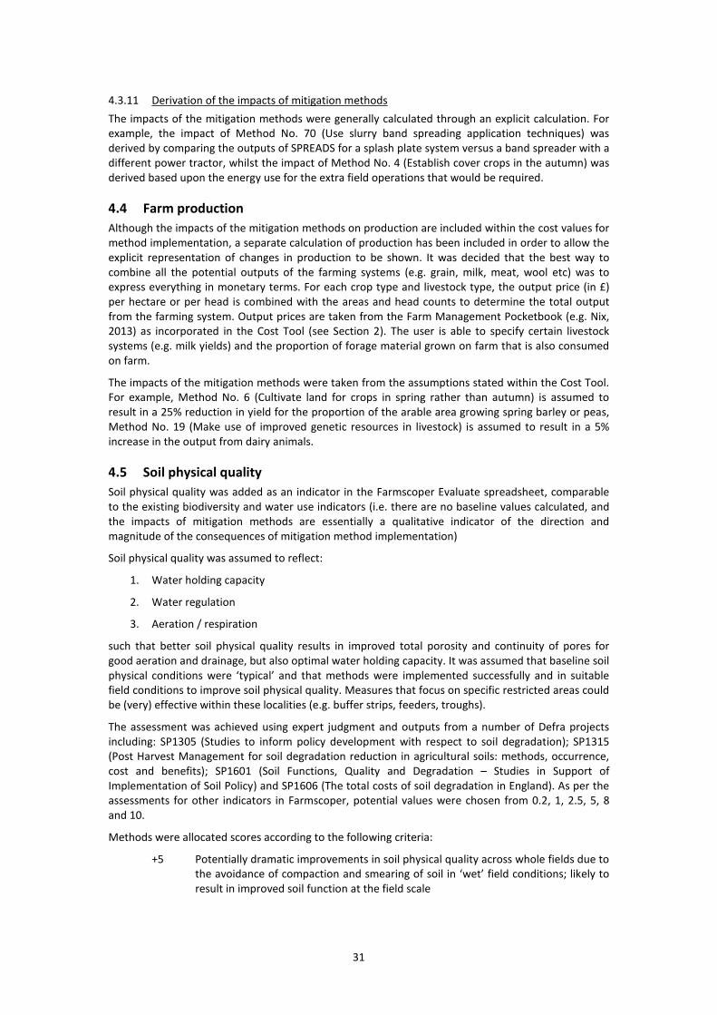
31
4.3.11 Derivation of the impacts of mitigation methods
The impacts of the mitigation methods were generally calculated through an explicit calculation. For
example, the impact of Method No. 70 (Use slurry band spreading application techniques) was
derived by comparing the outputs of SPREADS for a splash plate system versus a band spreader with a
different power tractor, whilst the impact of Method No. 4 (Establish cover crops in the autumn) was
derived based upon the energy use for the extra field operations that would be required.
4.4 Farm production
Although the impacts of the mitigation methods on production are included within the cost values for
method implementation, a separate calculation of production has been included in order to allow the
explicit representation of changes in production to be shown. It was decided that the best way to
combine all the potential outputs of the farming systems (e.g. grain, milk, meat, wool etc) was to
express everything in monetary terms. For each crop type and livestock type, the output price (in £)
per hectare or per head is combined with the areas and head counts to determine the total output
from the farming system. Output prices are taken from the Farm Management Pocketbook (e.g. Nix,
2013) as incorporated in the Cost Tool (see Section 2). The user is able to specify certain livestock
systems (e.g. milk yields) and the proportion of forage material grown on farm that is also consumed
on farm.
The impacts of the mitigation methods were taken from the assumptions stated within the Cost Tool.
For example, Method No. 6 (Cultivate land for crops in spring rather than autumn) is assumed to
result in a 25% reduction in yield for the proportion of the arable area growing spring barley or peas,
Method No. 19 (Make use of improved genetic resources in livestock) is assumed to result in a 5%
increase in the output from dairy animals.
4.5 Soil physical quality
Soil physical quality was added as an indicator in the Farmscoper Evaluate spreadsheet, comparable
to the existing biodiversity and water use indicators (i.e. there are no baseline values calculated, and
the impacts of mitigation methods are essentially a qualitative indicator of the direction and
magnitude of the consequences of mitigation method implementation)
Soil physical quality was assumed to reflect:
1. Water holding capacity
2. Water regulation
3. Aeration / respiration
such that better soil physical quality results in improved total porosity and continuity of pores for
good aeration and drainage, but also optimal water holding capacity. It was assumed that baseline soil
physical conditions were ‘typical’ and that methods were implemented successfully and in suitable
field conditions to improve soil physical quality. Measures that focus on specific restricted areas could
be (very) effective within these localities (e.g. buffer strips, feeders, troughs).
The assessment was achieved using expert judgment and outputs from a number of Defra projects
including: SP1305 (Studies to inform policy development with respect to soil degradation); SP1315
(Post Harvest Management for soil degradation reduction in agricultural soils: methods, occurrence,
cost and benefits); SP1601 (Soil Functions, Quality and Degradation – Studies in Support of
Implementation of Soil Policy) and SP1606 (The total costs of soil degradation in England). As per the
assessments for other indicators in Farmscoper, potential values were chosen from 0.2, 1, 2.5, 5, 8
and 10.
Methods were allocated scores according to the following criteria:
+5 Potentially dramatic improvements in soil physical quality across whole fields due to
the avoidance of compaction and smearing of soil in ‘wet’ field conditions; likely to
result in improved soil function at the field scale

32
+2.5 Moderate to large improvements in soil physical quality across whole fields
associated with improvements in soil structure and porosity due to either avoidance
or alleviation of soil compaction; can result in improved soil function at the field
scale
+1 Significant improvements in soil physical quality in specific localities (e.g. within a
riparian buffer strip); improved soil function in localised areas
-1 A small deterioration in soil quality may result due to greater likelihood of working
or trafficking soil in ‘wet’ conditions; can result in reduced soil function at the field
scale
-2.5 A moderate to large deterioration in soil physical quality due to greater likelihood of
grazing or trafficking when soils are 'wet'; likely to result in reduced soil function at
the field scale
-5 Potentially dramatic deterioration in soil quality over large areas due to livestock
poaching or compaction by machinery during harvest in late autumn; likely to result
in reduced soil function in multiple fields
The impact of methods on soil quality can vary according to soil type, mainly due to differences in clay
content, organic matter content, shrink-swell characteristics and the generally greater resilience and
resistance of heavier soils. Although Farmscoper recognizes different soil types, it was not possible to
link these directly to the impacts of the mitigation methods on soil quality. Therefore the impact value
was selected based upon the soil type most appropriate for that mitigation method (e.g. cover crops
are mostly grown on lighter soils).
4.6 Environmental Benefit
The environmental benefit calculation attempts to put a monetary value on the pollutant reductions
achieved through mitigation method implementation. This is achieved by calculating the units of each
pollutant saved in a mitigation scenario (calculated relative to the prior implementation situation) and
then multiplying these reductions with a value in £ per unit for each pollutant and then totalling
across all pollutants.
The default values for environmental benefit per unit pollutant emission reduced are shown in Table
4-12. Farmscoper has the capacity to use benefit values for pesticides and FIOs, but no default values
are provided for these two pollutants.
Table 4-12 Values used in the calculation of environmental benefit. The central value is the one
provided as a default value in Farmscoper. The low and high values are quoted to give an estimate
of the uncertainty.
Pollutant Units Low Central High
Nitrate £ kg-1 NO3-N 0.69 0.97 1.26
Phosphorus £ kg-1 P 26.66 33.16 39.34
Sediment £ kg-1 SS 0.30 0.39 0.49
Ammonia £ kg-1 NH3-N 2.17 2.79 3.17
GHGs £ kg-1 CO2-e 0.03 0.06 0.10
The values for nitrate, phosphorus and sediment are taken from Chadwick et al (2006). This project
estimated the economic damage from water pollutants across a range of ecosystem goods and
services (e.g. drinking water quality, fishing, bathing water quality and eutrophication) and isolated
the contribution of agriculture. There is considerable uncertainty in the costs for these different goods
and services, for example reducing freshwater eutrophication has a potential benefit of between
£168m and £330m per annum (Chadwick et al, 2006). Anthony et al (2008), summarising the results in
Spencer et al (2008) and Baker et al (2007) used costs for nitrate of £0.21 kg-1 and £0.67 kg-1,
phosphorus of £9.59 kg-1 and £44.93 kg-1 and sediment of £0.02 kg-1 and £0.11 kg-1, where the large
difference in values for each pollutant is due to uncertainty over the willingness to pay for achieving
good ecological status. These large uncertainties arise from the difficulty in estimating the costs for

33
treatment or the value of the benefits, apportioning the costs between the different pollutants (e.g.
how much of eutrophication is attributable to nitrate pollution) and then determining the proportion
of each pollutant which can be attributed to agriculture. It must also be noted that this simple costing
per unit of pollution reduced assumes that all reductions are equally beneficial, whereas reductions in
relatively pristine waters may not be as beneficial as the same reductions in more polluted waters.
There is also no relationship to pollutant concentrations, when these are the drivers for classification
under the EU water framework directive.
Farmscoper predicts energy use in terms of CO2-equivalent. It is possible to convert both methane
and nitrous oxide into CO2-e using global warming potentials of 21 and 310 CO2-e per kg respectively.
Thus all three of these pollutants can use the GHG figure from Table 4-12Error! Reference source not
found.. The unit value is the non-traded cost of carbon (DECC, 2011), which reflects the cost of
mitigating GHG emissions.
The value for ammonia is taken from air quality damage costs (Defra, 2011), and reflects the impacts
of exposure to air pollution on human health.
Note that the reports quoted are from different years, and thus the final values incorporated in
Farmscoper have been modified for consistency to reflect a value for 2013.

34
5 Review of prior implementation rates
The Farmscoper tool allows the user to enter an estimate of the present uptake of a method, which is
normally expressed as a percentage of the applicable area or number of livestock or number of farm
holdings. For example, the uptake of cover crops is expressed as a percent of the area of over-winter
bare ground or stubbles preceding spring sown crops, and the uptake of covered slurry stores is
expressed as a percent of the dairy and pig holdings managing their livestock manures as slurry.
A simple scoring system (Table 5-1) was used to estimate the possible range of uptake as it reflects
the uncertainty in mapping farm practice survey questions to the specific mitigation methods.
Responses to survey questions on practices may be unreliable because of misinterpretation by the
respondent, and because the questions rarely address the frequency and quality of uptake. For
example, a positive response to the question “Do you practice cover cropping?” provides no
information on the proportion of the field area affected or the timing or success in establishing a
cover crop.
The range of scores also closely resemble the ninety-five percent confidence intervals for a binomial
sample from a population of c. 50 farms with the listed average percent uptake. When used to
estimate mitigation potential for a catchment it is often forgotten that estimates of prior uptake are
derived from national stratified surveys of farm practice. The reported values are a good estimate of
uptake for a large population of farms, often many thousands, but a catchment study area may only
be 10 to 100 km2 in area and contain no more than 20 to 200 individual farms. The uptake of a specific
practice, such as ’site solid manure heaps away from watercourses/field drains’, can be either 0% or
100% at the scale of the individual farm. Unless you know otherwise, the farms within the catchment
are a random sample of the national population of farms and it is feasible that none or all carry out a
method, even if a national survey reports that 50% of farms practice it.
The scores therefore reflect a useful range for optimistic and pessimistic scenarios of mitigation
uptake based on the interpretation of survey questions, and also a range for uncertainty in prior
implementation within study catchments.
Table 5-1 Scoring system for assessing typical values and the range of percent uptake of mitigation
methods.
Score Typical Value Range
A 0 0
B 2 1-5
C 10 6-15
D 25 16-35
E 50 36 to 65
F 80 66 to 95
G 100 100
The available survey data relevant to the uptake off all the different mitigation methods was collated,
drawing upon the Defra Farm Practice Surveys in particular as these are exclusively for farms in
England, with a focus on survey data collated in the period 2006 to 2012. Survey data from other
parts of the United Kingdom was occasionally referenced where it has been reported by farm type,
allowing extrapolation to farm system types in England.
To aide the interpretation and synthesis of the survey data, the mitigation methods have been placed
into management groups to (Table 5-2), with the following subsections discussing the different
management groups. Based upon the survey data, each mitigation method was assigned an uptake
score (A to F; Table 5-1) for free draining and slowly permeable soil types, along with any expected
variation in uptake between more intensive and extensive systems, or between farms with and
without grazing livestock. The results of the process are presented in Table 5-3. Note that there was
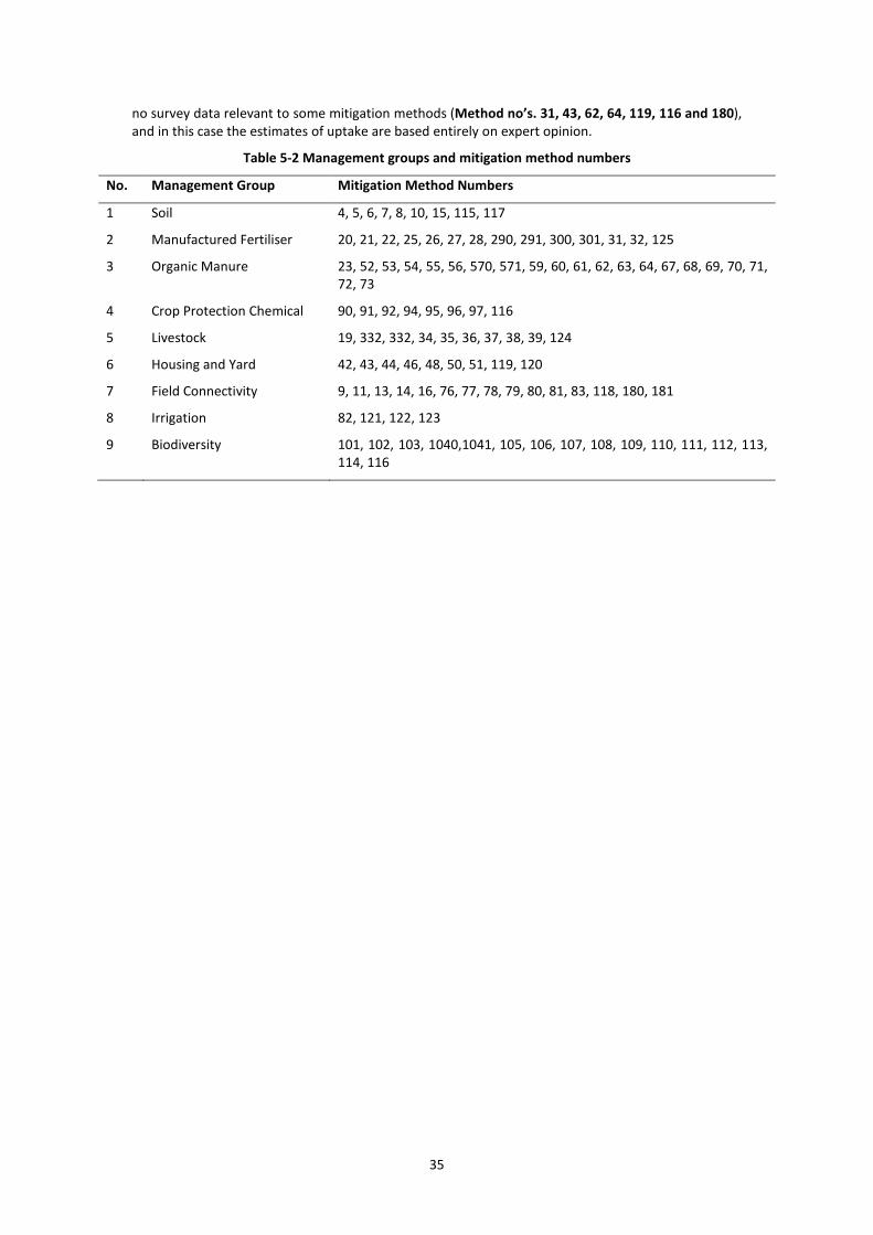
35
no survey data relevant to some mitigation methods (Method no’s. 31, 43, 62, 64, 119, 116 and 180),
and in this case the estimates of uptake are based entirely on expert opinion.
Table 5-2 Management groups and mitigation method numbers
No. Management Group Mitigation Method Numbers
1 Soil 4, 5, 6, 7, 8, 10, 15, 115, 117
2 Manufactured Fertiliser 20, 21, 22, 25, 26, 27, 28, 290, 291, 300, 301, 31, 32, 125
3 Organic Manure 23, 52, 53, 54, 55, 56, 570, 571, 59, 60, 61, 62, 63, 64, 67, 68, 69, 70, 71,
72, 73
4 Crop Protection Chemical 90, 91, 92, 94, 95, 96, 97, 116
5 Livestock 19, 332, 332, 34, 35, 36, 37, 38, 39, 124
6 Housing and Yard 42, 43, 44, 46, 48, 50, 51, 119, 120
7 Field Connectivity 9, 11, 13, 14, 16, 76, 77, 78, 79, 80, 81, 83, 118, 180, 181
8 Irrigation 82, 121, 122, 123
9 Biodiversity 101, 102, 103, 1040,1041, 105, 106, 107, 108, 109, 110, 111, 112, 113,
114, 116

36
Table 5-3 Mitigation methods and agreed levels of prior uptake representing the present day, circa 2010. The modifiers refer to the lettered categories, such that a ‘C’
baseline value modified by -1 becomes a ‘B’. Note that implementation rates for methods named in italics are based solely on expert opinion.
Group
ID
Method Name
Baseline Values Modifiers
Free
Draining
Other
Soils NVZ
Intensive
Grazing
Extensive
grazing
1 4 Establish cover crops in the autumn C B -1 -1
1 5 Early harvesting and establishment of crops in the autumn E E
1 6 Cultivate land for crops in spring rather than autumn F B
1 7 Adopt reduced cultivation systems C E -1 -1
1 8 Cultivate compacted tillage soils D D -1 -1
7 9 Cultivate and drill across the slope D C
1 10 Leave autumn seedbeds rough D D -1 -1
7 11 Manage over-winter tramlines D D -1 -1
7 13 Establish in-field grass buffer strips B B
7 14 Establish riparian buffer strips D D -1 -1
1 15 Loosen compacted soil layers in grassland fields C C
7 16 Allow grassland field drainage systems to deteriorate A B
7 180 Ditch management on arable land A E
7 181 Ditch management on grassland A D
5 19 Make use of improved genetic resources in livestock C C
2 20 Use plants with improved nitrogen use efficiency A A
2 21 Fertiliser spreader calibration E E 1 -1
2 22 Use a fertiliser recommendation system F F 1 -1
3 23 Integrate fertiliser and manure nutrient supply E E 1 -1
2 25 Do not apply manufactured fertiliser to high-risk areas E E 1 -1
2 26 Avoid spreading manufactured fertiliser to fields at high-risk times F* F* 1

37
Group
ID
Method Name
Baseline Values Modifiers
Free
Draining
Other
Soils NVZ
Intensive
Grazing
Extensive
grazing
2 27 Use manufactured fertiliser placement technologies C C
2 28 Use nitrification inhibitors A A
2 290 Replace urea fertiliser to grassland with another form A A
2 291 Replace urea fertiliser to arable land with another form A A
2 300 Incorporate a urease inhibitor into urea fertilisers for grassland B B -1
2 301 Incorporate a urease inhibitor into urea fertilisers for arable land B B -1
2 31 Use clover in place of fertiliser nitrogen D* D*
2 32 Do not apply P fertilisers to high P index soils A A
5 331 Reduce dietary N and P intakes: Dairy C C
5 332 Reduce dietary N and P intakes: Pigs F F
5 333 Reduce dietary N and P intakes: Poultry F F
5 34 Adopt phase feeding of livestock F F
5 35 Reduce the length of the grazing day/grazing season C C
5 36 Extend the grazing season for cattle C C
5 37 Reduce field stocking rates when soils are wet E E
5 38 Move feeders at regular intervals E E
5 39 Construct troughs with concrete base B B
6 42 Increase scraping frequency in dairy cow cubicle housing C C
6 43 Additional targeted bedding for straw-bedded cattle housing C C
6 44 Washing down of dairy cow collecting yards D D
6 46 Frequent removal of slurry from beneath-slat storage in pig housing B B
6 48 Install air-scrubbers or biotrickling filters in mechanically ventilated pig housing B B
6 50 More frequent manure removal from laying hen housing with manure belt systems C C

38
Group
ID
Method Name
Baseline Values Modifiers
Free
Draining
Other
Soils NVZ
Intensive
Grazing
Extensive
grazing
6 51 In-house poultry manure drying C C
3 52 Increase the capacity of farm slurry stores to improve timing of slurry applications A A 1
3 53 Adopt batch storage of slurry A A
3 54 Install covers to slurry stores C C
3 55 Allow cattle slurry stores to develop a natural crust F F
3 56 Anaerobic digestion of livestock manures A A
3 570 Minimise the volume of dirty water produced (sent to dirty water store) D D -1
3 571 Minimise the volume of dirty water produced (sent to slurry store) D D -1
3 59 Compost solid manure B B
3 60 Site solid manure heaps away from watercourses/field drains F E 1
3 61 Store solid manure heaps on an impermeable base and collect effluent C C
3 62 Cover solid manure stores with sheeting B B
3 63 Use liquid/solid manure separation techniques B B
3 64 Use poultry litter additives A A
3 67 Manure Spreader Calibration D D 1 -1
3 68 Do not apply manure to high-risk areas F F 1 -1
3 69 Do not spread slurry or poultry manure at high-risk times D* D* 1 -1
3 70 Use slurry band spreading application techniques C C -1
3 71 Use slurry injection application techniques B B -1
3 72 Do not spread FYM to fields at high-risk times D* D* 1 -1
3 73 Incorporate manure into the soil C C -1
7 76 Fence off rivers and streams from livestock E E -1
7 77 Construct bridges for livestock crossing rivers/streams F F

39
Group
ID
Method Name
Baseline Values Modifiers
Free
Draining
Other
Soils NVZ
Intensive
Grazing
Extensive
grazing
7 78 Re-site gateways away from high-risk areas A A
7 79 Farm track management E E -1
7 80 Establish new hedges B B
7 81 Establish and maintain artificial wetlands - steading runoff A B
8 82 Irrigate crops to achieve maximum yield D B
7 83 Establish tree shelter belts around livestock housing C C
4 90 Calibration of sprayer F F -1
4 91 Fill/Mix/Clean sprayer in field E E -1
4 92 Avoid PPP application at high risk timings E D -1
4 94 Drift reduction methods E E -1
4 95 PPP substitution B B -1
4 96 Construct bunded impermeable PPP filling/mixing/cleaning area C C -1
4 97 Treatment of PPP washings through disposal, activated carbon or biobeds F F -1
9 101 Protection of in-field trees C C
9 102 Management of woodland edges B B
9 103 Management of in-field ponds B B
9 105 Management of arable field corners C C
9 106 Plant areas of farm with wild bird seed / nectar flower mixtures C C
9 107 Beetle banks B B
9 108 Uncropped cultivated margins B B
9 109 Skylark plots B B
9 110 Uncropped cultivated areas B B
9 111 Unfertilised cereal headlands B B

40
Group
ID
Method Name
Baseline Values Modifiers
Free
Draining
Other
Soils NVZ
Intensive
Grazing
Extensive
grazing
9 112 Unharvested cereal headlands B B
9 113 Undersown spring cereals B B
9 114 Management of grassland field corners B B
1 115 Leave over winter stubbles F B
4 116 Leave residual levels of non-aggressive weeds in crops B B
1 117 Use correctly-inflated low ground pressure tyres on machinery E E -1 -1
7 118 Locate out-wintered stock away from watercourses C C
6 119 Use dry-cleaning techniques to remove solid waste from yards prior to cleaning A A -1
6 120 Capture of dirty water in a dirty water store F F -1
8 121 Irrigation/water supply equipment is maintained and leaks repaired E C
8 122 Avoid irrigating at high risk times D B
8 123 Use efficient irrigation techniques (boom trickle, self-closing nozzles) C A
5 124 Use high sugar grasses C C
2 125 Monitor and amend soil pH status for grassland A A
5 126 Increased use of maize silage A A
* Current implementation for these methods was accounted for within the baseline modelling, as specification of the appropriate model input data was based upon
the British Survey of Fertiliser Practice and thus would already include any adjustments for avoiding high risk times or using clover. Thus a value of A is actually used
within Farmscoper.

41
5.1 Soil Management
Soil management mitigation methods are principally concerned with protecting the soil from erosive
rainfall by maintaining vegetative cover, and preventing or removing soil compaction or poaching that
can result in increased surface runoff and mobilisation of soil and soluble pollutants.
There is a history of recording observations of soil erosion and actions taken to prevent soil erosion
dating back to the very first Defra Farm Practice Survey (2001). Early surveys focused on actions to
prevent soil damage or control runoff, such as delaying cultivations or contour ploughing. The most
recent surveys have focussed on the assessment of soil structure and actions taken to remove soil
compaction after it has occurred.
Cover crops and stubble protect the soil from erosive rainfall impact, and also remove nutrients from
the soil that would otherwise be at risk of leaching. The Defra Farm Practice Survey (2010) special
survey of over-winter cover on c. 10,500 holdings reported that 81,000 ha were purposely sown with
cover crops in the winter of 2009/10. This represented c. 10% of the area of relevant spring crops
(spring barley, maize, sugar beet, peas, vegetables and potatoes) (Method no. 4). However, it is
possible that the reported over-winter cover included forage crops such as stubble turnips, in which
case poaching caused by grazing livestock may enhance runoff and soil erosion, and the area of
effective arable cropping is less. The survey also reported that 514,000 ha of land was covered with
crop residues or stubble from the previous harvest. This represented c. 13% of the total arable crop
area or 67% of the relevant spring crop area (Method no. 115). According to Environment
Stewardship scheme summary statistics (correct as of 2012) the total paid option area of over-
wintered stubble is 107,510 ha (Lindsey Clothier, pers. comm.). The Defra (2012) Survey of Land
Managed Under the Campaign for the Farmed Environment estimated that 98,506 ha of arable land
was under over-wintered stubble as unpaid environmental management. These values are
considerably less than reported by the Defra (2010) Farm Practice Survey, indicating that a relatively
small proportion of over-wintered stubbles are in Environmental Stewardship or registered with the
Campaign for the Farmed Environment (CFE).
Reduced tillage can improve the structure of soils, resulting in improved water infiltration and
reduced erosion. The Defra (2010) Farm Practice Survey reported that 40% of the total cultivated area
was managed using reduced or minimum tillage, and 4% by zero tillage (Method no. 7). The Defra
(2008) Farm Practice Survey similarly reported that 49% of farms had used reduced or shallow
cultivation systems in the past 12 months, and the Defra Farm Business Survey reported that 38% of
cropping farms and 4% of livestock farms had practised minimum tillage to prevent diffuse pollution.
The Defra Farm Practice Survey (2007) reported that minimum tillage was practised on 52% of cereal
farms, 17% of dairy farms, and less than 12% of grazing livestock farms.
Autumn cultivation of land stimulates the mineralisation of nitrogen from organic matter reserves at a
time when there is little or no uptake by the crop, resulting in increased risk of nitrate leaching. By
cultivating in spring the risk of leaching is reduced and nitrogen mineralised from spring cultivation is
available for uptake by the following spring crops. The Defra Farm Practice Survey (2007) reported
that 25% of cereal farms, 10% of dairy farms, and less than 5% of grazing livestock farms had changed
the timing of cultivations to reduce the risk of diffuse pollution (Method no. 6). Anthony et al. (2012)
reported that between 44 and 50% of 218 livestock farms with arable land surveyed in Wales
specifically delayed cultivation for spring crops until spring. This value may be higher than for England
due to the dominance of medium-textured soils and a higher proportion of spring sown crops.
For autumn sown crops, early harvesting of the previous crop allows better establishment to take up
soil nutrients and development of some over-winter crop cover to protect against erosive rainfall.
Early harvesting of crops also avoids the risk of soil compaction due to machinery operations on ‘wet’
soil. Anthony et al. (2012) reported that between 19 and 24% of 218 livestock farms with arable land
surveyed in Wales had established winter cover through early drilling (Method no. 5).
Compacted soil layers reduce water infiltration, and increase surface runoff and soil erosion risk. Use
of low ground-pressure vehicles can limit soil compaction. The Defra Farm Practice Survey (2008)
recorded that 61% of 1,180 holdings had used low ground pressure set-ups within the last 12 months
to reduce soil compaction. Uptake was highest in the East Midlands (71%) and East of England (76%),
and lowest in the South West (48%) and North West (52%), indicative of an effect of farm type. The

42
Defra Farm Practice Survey (2012) reported that 54% of holdings had used low ground pressure set-
ups, and this varied from a low of 26% for the grazing livestock farm type to a high of 77% for the
specialist cereal farm type (Method no. 117).
Some degree of soil compaction is an inevitable outcome of a long-history of machinery operations or
trampling by livestock or cultivating and harvesting under adverse weather conditions. However,
there are methods available to disrupt and remove compaction. The Defra (2012) Farm Practice
Survey reported that 47% of farms carried out a soil structure survey prior to cultivation or any other
soil husbandry activity. However, the majority (28%) only surveyed where there was obvious
compaction and 53% did not carry out any survey. The percent of farms that did not carry out any
survey varied from 31% for the specialist cereal farm type, through 52% for dairy, to 75% for grazing
livestock farm types. This therefore represents a limit to the proportion of farms that can effectively
monitor and remove soil compaction.
The Defra (2012) Farm Practice Survey reported that 66% of holdings removed headland compaction
after harvest (ranging from 15% for grazing livestock farms to 87% for the specialist cereal farm type)
and 30% of grazing livestock farms removed grassland compaction by turf lifting or spiking (Method
no. 8 and 15). Anthony et al. (2012) similarly reported that between 22 and 25% of 218 livestock
farms with arable land surveyed in Wales had practised rough ploughing to remove harvest
compaction (Method No. 10). Also, between 34 and 46% of 590 livestock farms with improved
grassland had removed soil compaction on grassland by re-seeding or soil loosening.
Soil nutrients are at their maximum availability to plants in slightly acidic, neutral or slightly alkaline
soils. Agricultural practices often decrease the pH of a soil, and regular soil pH testing and treatment
with lime if necessary will improve the response of crops and grass to applied fertiliser. The Defra
Farm Practice Survey (2012) reported that 70% of farms tested the pH of soil at least every five years,
and 22% of farms more than every three years (Method no. 125).
5.2 Manufactured Fertiliser Management
Manufactured fertiliser management mitigation methods are principally concerned with ensuring that
only the required quantity of fertiliser is applied and only at the correct time to meet crop demand,
therefore avoiding the risk of surplus nutrients being mobilised.
The British Survey of Fertiliser Practice surveys fertiliser application rates and the methods and timing
of application nationally each year, whilst the Defra Farm Practice Surveys have collected information
on the sources of advice and tools used by farmers to plan fertiliser applications appropriately, taking
account of the history of land management, soil nutrient status and crop requirements.
The British Survey of Fertiliser Practice was used to define fertiliser practices for input to the diffuse
pollution models that underpin Farmscoper. As a result the baseline estimates of pollutant losses will
have captured the range of present day fertiliser practice, including the timing and types of fertiliser
used. Therefore, the prior uptake of the mitigation method to avoid spreading manufactured fertiliser
at high-risk times is zero (Method no. 26). Similarly, the prior uptake of alternatives to urea fertiliser
is zero (Method no. 290 and 291). According to the British Survey of Fertiliser Practice (2010) 9% of all
tillage land and 3% of all improved grassland receives urea fertiliser. This is also the maximum
potential uptake of urease inhibitors (Method no. 300 and 301). The uptake of nitrification inhibitors
is also very low, although no reliable information is available at present (Method no. 28). The uptake
of plants with improved genetic traits and nitrogen use efficiency is also assumed to be zero as
present breeding practices do not select for nitrogen efficiency (Method no. 20).
Nutrient and manure management planning involve calculating the balance of crop nutrient
requirements and availability from the soil, manufactured fertilisers and organic manures. It is an
effective method to optimise crop yields and maximise nutrient uptake and to avoid surplus nutrient
applications that are at increased risk of leaching. The Defra (2013) Farm Practice Survey reported
that 57% of farms had a nutrient management plan, accounting for 73% of the farmed area. The
farmer created the majority with the help of a professional (48%) or by an advisor or contractor
(27%). According to the earlier Defra (2012) Farm Practice Survey the majority of farmers use the
Tried and Tested paper based planning system (16%) or PLANET (48%) software when calculating the
fertiliser requirements of crops (Method no. 22). Note that use of a fertiliser recommendation system

43
may actually result in increased fertiliser application rates, where crops were initially under fertilised
– this would probably result in increased leaching and emissions. However, Farmscoper only
represents the more common situation where fertiliser usage would be reduced.
The Defra (2013) Farm Practice Survey also reported that 71% of farms had a manure management
plan, and that 57% of farms assess or calculate the value of their manure, and 24% test the nutrient
content by taking samples. According to the Defra (2012) Farm Practice Survey, between 31 and 46%
of specialist cereal farms use Global Positioning Systems, soil mapping or variable rate applications in
contrast to between 3 and 11% of grazing livestock farms. The existence of nutrient and manure
management plans, together with the growing adoption of precision farming techniques, should also
significantly reduce the risk of nutrient applications in excess of crop or soil requirements (Method
no. 25).
Balancing crop requirements specifically requires knowledge of the soil nutrient supply. According to
the Defra (2012) Farm Practice Survey, around 95% of specialist cereal farms test their soils for
nutrient status at least every five years, in comparison to 77% of dairy farms and less than 43% of
grazing livestock farms. The Defra Farm Business Survey (2009/10) similarly reported that testing soil
nutrient levels was practised on 79% of cropping farms and 35% of grazing livestock farms. However,
this testing should result in a smaller area of high P index soils (which is an applicability constraint),
rather than a higher level of uptake. Therefore implementation is set to zero for Method no. 32.
Effective implementation of a nutrient management plan also requires calibration of fertiliser
spreaders to avoid inaccurate spreading and the risk of under and over application. The Defra (2011)
Farm Practice Survey reported that 27% of holdings check and calibrate the spread pattern of their
spreaders more than once a year and 56% check and correct the rate for fertiliser type more than
once a year. The effective calibration rate may be higher in areas where contractors carry out the
majority of manure spreading. According to the British Survey of Fertiliser Practice (2005 to 2009),
around 40% of farms test their fertiliser spreaders at least once per year, and between 5 and 10% test
at each change of fertiliser type (Method no. 21).
Placement of nutrients close to germinating seed or the roots of established crops can help enhance
nutrient uptake, and can also reduce the exposure of fertiliser at the soil surface, thereby reducing
the risk of incidental losses in surface runoff. Nitrogen fertiliser placement is widely used for maize,
potatoes and some horticultural crops, e.g. strawberries. By comparison with the total area of arable
and horticultural crops (Defra, 2010) uptake is no more than 5% (Method no. 27).
The nitrogen at risk of leaching can be reduced directly by using clover in a grass sward to fix nitrogen
from the air in place of manufactured fertiliser inputs. The Defra Farm Practice Surveys (2011 and
2012) also reported that 79% of livestock holdings had sown a proportion of their temporary
grassland with a clover mix, and 33% had sown all of their temporary grassland with a clover mix. The
use of clover will have been reflected in lower rates of nitrogen fertiliser application reported by the
British Survey of Fertiliser Practice – as this is used as the baseline fertiliser rates for the model farms,
this implementation is already reflected within the default farm systems and so the prior
implementation rate for the method itself is 0 (Method no. 31).
5.3 Organic Manure Management
Organic manure management mitigation methods are principally concerned with estimating the
nutrient content of manures, and maximising the nutrient use efficiency by improved application
methods and planned timing and placement to avoid both gaseous emissions and surface runoff or
leaching.
As for manufactured fertiliser, the British Survey of Fertiliser Practice was used to define manure
application rates and timing for input to the diffuse pollution models that underpin Farmscoper. The
current timing of manure applications to land are therefore part of the Farmscoper baseline, and by
definition the further uptake of practices to avoid high risk times is zero (Method no. 69 and 72)
except within the Nitrate Vulnerable Zone area where closed periods for manure application are
enforced and uptake rates for some methods are higher.
The Defra Farm Practice Surveys have a history of collecting information on the types of manure
storage and the adoption of specific technologies for manure application. The focus has been on the
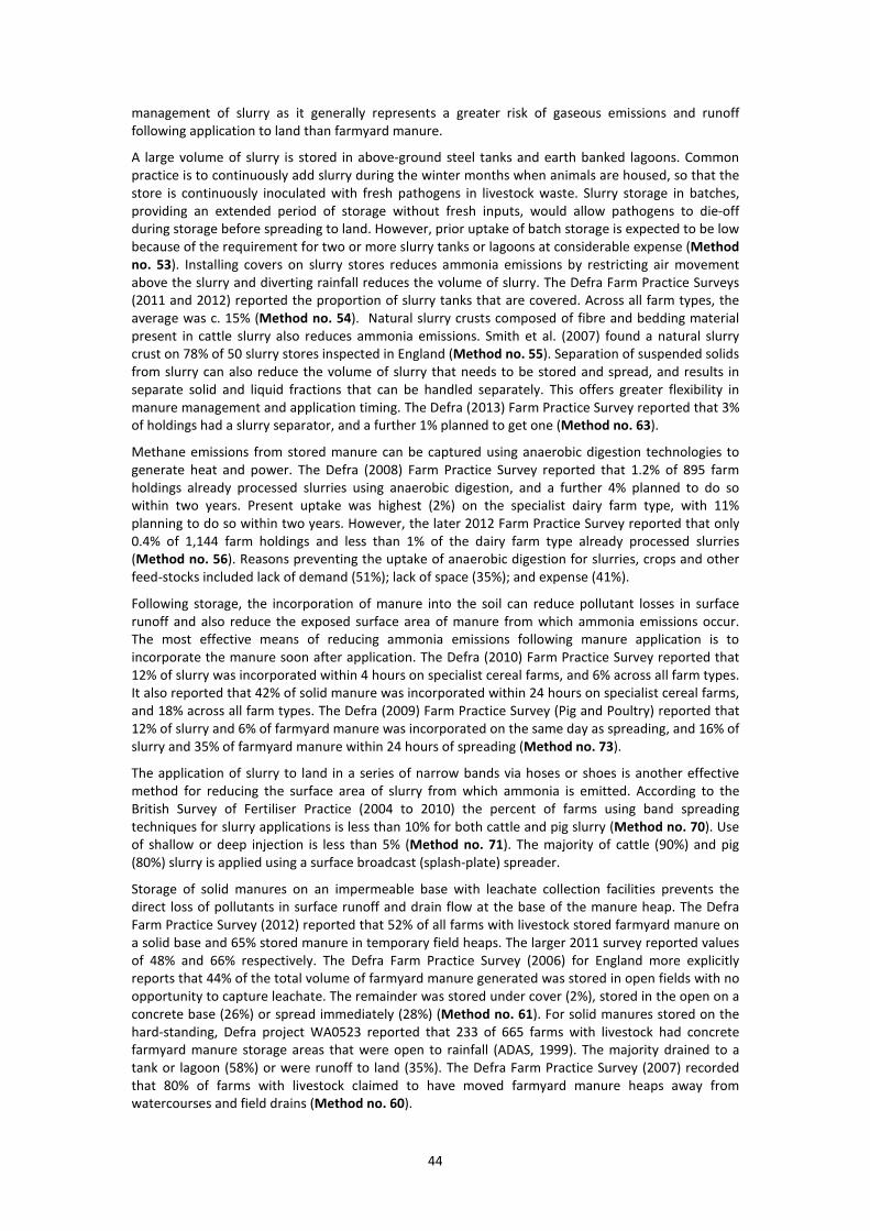
44
management of slurry as it generally represents a greater risk of gaseous emissions and runoff
following application to land than farmyard manure.
A large volume of slurry is stored in above-ground steel tanks and earth banked lagoons. Common
practice is to continuously add slurry during the winter months when animals are housed, so that the
store is continuously inoculated with fresh pathogens in livestock waste. Slurry storage in batches,
providing an extended period of storage without fresh inputs, would allow pathogens to die-off
during storage before spreading to land. However, prior uptake of batch storage is expected to be low
because of the requirement for two or more slurry tanks or lagoons at considerable expense (Method
no. 53). Installing covers on slurry stores reduces ammonia emissions by restricting air movement
above the slurry and diverting rainfall reduces the volume of slurry. The Defra Farm Practice Surveys
(2011 and 2012) reported the proportion of slurry tanks that are covered. Across all farm types, the
average was c. 15% (Method no. 54). Natural slurry crusts composed of fibre and bedding material
present in cattle slurry also reduces ammonia emissions. Smith et al. (2007) found a natural slurry
crust on 78% of 50 slurry stores inspected in England (Method no. 55). Separation of suspended solids
from slurry can also reduce the volume of slurry that needs to be stored and spread, and results in
separate solid and liquid fractions that can be handled separately. This offers greater flexibility in
manure management and application timing. The Defra (2013) Farm Practice Survey reported that 3%
of holdings had a slurry separator, and a further 1% planned to get one (Method no. 63).
Methane emissions from stored manure can be captured using anaerobic digestion technologies to
generate heat and power. The Defra (2008) Farm Practice Survey reported that 1.2% of 895 farm
holdings already processed slurries using anaerobic digestion, and a further 4% planned to do so
within two years. Present uptake was highest (2%) on the specialist dairy farm type, with 11%
planning to do so within two years. However, the later 2012 Farm Practice Survey reported that only
0.4% of 1,144 farm holdings and less than 1% of the dairy farm type already processed slurries
(Method no. 56). Reasons preventing the uptake of anaerobic digestion for slurries, crops and other
feed-stocks included lack of demand (51%); lack of space (35%); and expense (41%).
Following storage, the incorporation of manure into the soil can reduce pollutant losses in surface
runoff and also reduce the exposed surface area of manure from which ammonia emissions occur.
The most effective means of reducing ammonia emissions following manure application is to
incorporate the manure soon after application. The Defra (2010) Farm Practice Survey reported that
12% of slurry was incorporated within 4 hours on specialist cereal farms, and 6% across all farm types.
It also reported that 42% of solid manure was incorporated within 24 hours on specialist cereal farms,
and 18% across all farm types. The Defra (2009) Farm Practice Survey (Pig and Poultry) reported that
12% of slurry and 6% of farmyard manure was incorporated on the same day as spreading, and 16% of
slurry and 35% of farmyard manure within 24 hours of spreading (Method no. 73).
The application of slurry to land in a series of narrow bands via hoses or shoes is another effective
method for reducing the surface area of slurry from which ammonia is emitted. According to the
British Survey of Fertiliser Practice (2004 to 2010) the percent of farms using band spreading
techniques for slurry applications is less than 10% for both cattle and pig slurry (Method no. 70). Use
of shallow or deep injection is less than 5% (Method no. 71). The majority of cattle (90%) and pig
(80%) slurry is applied using a surface broadcast (splash-plate) spreader.
Storage of solid manures on an impermeable base with leachate collection facilities prevents the
direct loss of pollutants in surface runoff and drain flow at the base of the manure heap. The Defra
Farm Practice Survey (2012) reported that 52% of all farms with livestock stored farmyard manure on
a solid base and 65% stored manure in temporary field heaps. The larger 2011 survey reported values
of 48% and 66% respectively. The Defra Farm Practice Survey (2006) for England more explicitly
reports that 44% of the total volume of farmyard manure generated was stored in open fields with no
opportunity to capture leachate. The remainder was stored under cover (2%), stored in the open on a
concrete base (26%) or spread immediately (28%) (Method no. 61). For solid manures stored on the
hard-standing, Defra project WA0523 reported that 233 of 665 farms with livestock had concrete
farmyard manure storage areas that were open to rainfall (ADAS, 1999). The majority drained to a
tank or lagoon (58%) or were runoff to land (35%). The Defra Farm Practice Survey (2007) recorded
that 80% of farms with livestock claimed to have moved farmyard manure heaps away from
watercourses and field drains (Method no. 60).

45
The Defra (2012) Farm Practice Survey reported that 57% of farms had a nutrient management plan,
accounting for 73% of the farmed area. The farmer created the majority with the help of a
professional (48%) or by an advisor or contractor (27%). The nutrient management plan would help
farmers account for the nutrient value of organic manures when balancing crop requirements and
thereby reduce manufactured fertiliser applications. However, the Defra (2012) Farm Practice Survey
reported that only 57% of farms assess or calculate the value of their manures, and only 24% tested
the nutrient content by taking samples (Method no. 23). The Defra (2013) Farm Practice Survey also
reported that on over half of holdings (58%) where the farmer spreads manure or slurry himself the
manure or slurry spreader is never calibrated (Method no. 67).
A manure management plan includes a map of field areas that must be avoided due to slope, soil type
and proximity to water. According to the Defra (2012) Farm Practice Survey, 65% of grazing livestock
farms had a manure management plan and 90% of dairy farms (Method no. 68).
5.4 Crop Protection Chemical Management
Crop protection management mitigation methods are principally concerned with minimising the risk
of small quantities of chemicals entering watercourses from machinery washings or spray drift whilst
treating a crop.
Chemical sprayer practice in the United Kingdom was most recently surveyed by ADAS on behalf of
the Health and Safety Executive Chemical Regulations Directorate (Twining and Simpson, 2009a). The
surveys sampled c. 2,260 farm holdings including booster surveys for Scotland and Wales (Twining
and Simpson, 2009b; 2009c). After appropriate weighting to represent the national composition of
farm types, the weighted base for the survey was 1,403 interviews of which 34% used pesticides.
Knapsack (64%) and tractor mounted or self-propelled boom sprayers (50%) are the most common
type of equipment used to apply pesticides in England. The majority of knapsack (62%) and boom
sprayers (79%) had been tested within the last year, although only 7% of knapsack and 50% of booms
had been tested through the National Sprayer Testing Scheme (Method no. 90).
High risk times are considered to be windy days on the day of application affecting losses via spray
drift, wet soil conditions on the day of application and the imminent occurrence of rainfall both of
which promote losses via surface runoff and drain flow. Twining and Simpson (2009a) report that the
factors most commonly taken into account by farmers when deciding when to apply pesticides were
wind speed (71%), forecast of rain (79%), crop growth stage (43%) and ground conditions (32%).
However, 35% of those who decided when to apply pesticides did not hold any relevant qualifications.
The larger arable farms were most likely to take key factors into account, and almost all contractors
(96%) took the forecast of rain into account (Method no. 92).
Strategies used for reducing spray drift varied between farmer and contractors (Twining and Simpson,
2009a). Farmers tended to rely more on spraying in low wind conditions (69%) than on no-spray
buffer strips (28%) or low drift nozzles (23%). Contractors were more likely to use no-spray buffer
strips (74%) and low drift nozzles (68%), in addition to spraying in low wind conditions (82%). As
pesticides are applied by the farmer or farm worker on a majority (67%) of farms, the overall adoption
of spray drift reduction methods is not as advanced as it would be if agricultural contractors
dominated pesticide applications (Method no. 94). The Farm Business Survey (2009/10)
independently recorded 48% of farm holdings that used pesticides employing high tech spray nozzles
to minimise spray drift.
Although it is believed that there is a high willingness amongst farmers to substitute chemicals for less
toxic or less mobile equivalents, the reliance on branded products and professional agronomists to
make the decision on which pesticide to apply means that the farmers do not have the necessary
information to carry this out (Method no. 95).
Twining and Simpson (2009a) report that 85% of holdings in England disposed of sprayer washings
correctly, with the majority of washings from the sprayer tank sprayed on appropriate crops (77%) or
on waste land (8%). Only a small proportion was collected by a waste contractor (5%) or stored (1%),
with no explicit reporting of the use of activated carbon or biobeds (Method no. 97). Cattle and
sheep farms were more likely to dispose of washings on wasteland rather than appropriate crops.

46
Supplementary information on the practices of sprayer filling and cleaning is available from an earlier
survey of sprayer practices on arable holdings in the United Kingdom carried out by Garthwaite
(2002). The survey was based on farm visits and a postal survey of c. 800 holdings. The data were
weighted by farm size and arable crop area to provide national estimates of sprayer practice.
Overall, 57% of pesticide filling for the arable area was conducted in the yard alone, with 15% taking
place in the field and 28% in both situations. Overall, 45% of sprayers were cleaned in the yard and
44% in the field. When weighted to the number of washes per year, 50% of sprayers were washed in
the field (Method no. 91). Only 4% of the arable area had a bunded area within the yard (Method no.
96). Drainage at the sprayer cleaning or filling area was to soil, rubble, wasteland or watercourse at c.
40 to 50% of holdings, as opposed to collection tanks, soak away or Environment Agency approved
areas.
5.5 Livestock Management
Livestock management mitigation methods are principally concerned with ensuring that animals are
fed appropriately to minimise the quantity of potential pollutants in excreta, and that the location of
grazing is controlled to prevent soil damage.
The older Defra Farm Practice Surveys have generally focussed on grazing management, and most
recently the Greenhouse Gas orientated surveys have started collecting data on feed management
and trait selection in livestock that has the potential to reduce overall livestock numbers and enteric
methane emissions whilst maintaining outputs.
The Defra Farm Practice Survey (2007) recorded that 43% of dairy farms and 54% of grazing livestock
farms claimed to move feeder and water troughs at regular intervals to avoid poaching and soil
damage around them. Similarly, Anthony et al. (2012) recorded that 44% of dairy farms and 50% of
cattle and sheep farms in Wales claimed to have re-located or regularly rotated feeding sites (Method
no. 38). Only 309 capital grants for concrete bases to water troughs are recorded under the Entry
Level and Higher Level Stewardship schemes in England (Lindsey Clothier, pers. comm.) (Method no.
39).
The Defra (2013) Farm Practice Survey reported that 23% of holdings breeding dairy cows always used
bulls with a high Profitable Lifetime Index (PLI), and bulls and rams with high Estimated Breeding
Values (EBV) were always used by 16% of holdings breeding beef cattle and 10% of those breeding
lambs. The latter holdings accounted for 24% of beef cattle and 11% of lambs (Method no. 19).
Reducing feed nitrogen intake results in a reduction in nitrogen excretion and an increase in nitrogen
use efficiency by dairy cattle. The Defra (2013) Farm Practice Survey reported that 73% of livestock
holdings used a ration formulation programme or took professional nutritional advice. This would be
a firm basis for reducing dietary nitrogen and phosphorus intakes for dairy stock. However, a
reduction in nitrogen intake frequently also results in a reduction in milk yield and there is little
financial incentive for farmers to reduce the dietary protein content for cows on grass silage based
diets (Cottrill et al., 2006) (Method no. 331). Sowing high sugar grasses can also result in improved
feed digestibility and nitrogen use efficiency by grazing livestock. The Defra Farm Practice Survey
(2013) reported that 38% of the temporary grassland area on livestock holdings was sown with high
sugar grasses (Method no. 124).
Phase feeding involves more precise matching of the ration to the nutrient requirement of groups of
animals, based on livestock growth stage, and results in lower nutrient excretion. Adoption of phase
feeding is believed to be implemented widely in the pig and poultry industry (Cottrill et al., 2006)
(Method no. 34). Similarly, the current uptake of phytase supplements that increase the availability of
dietary phosphorus is estimated to be already close to the potential as including the enzyme in the
diet is cost neutral. Industry sources indicate that phytase is incorporated into approximately 90% of
pig diets, 90% of hen feeds and 40% of broiler rations manufactured in the UK (Cottrill et al., 2006)
(Method no. 332).
Changes to the length of time livestock graze in fields can affect the balance of gaseous emissions
from managed manures and excreta at grazing and the risk of soil damage and erosion, especially if
livestock are grazed early or late in the year when soils are ‘wet’. It is estimated that c. 10% of dairy
farms in England are aiming to strategically reduce the length of the grazing season, and a similar

47
proportion are aiming to extend the season (Method no. 35 and 36). The changes are in response to
herd size, forage availability, animal welfare and economic factors that are individual to each farm.
Both strategies are distinct from the tactical reduction in field stocking rates when fields are wet. The
Defra Farm Practice Survey (2005) reported that 56% of livestock farms delayed putting stock out to
grass to avoid field poaching in a typical year, and 60% took stock off the land to avoid poaching. The
Defra Farm Practice Survey (2008) reported that 89% of livestock farms claimed to have delayed turn
out of animals to avoid poaching, and 27% had added additional housing to facilitate this (Method no.
37).
5.6 Housing and Yard Management
Housing and yard management mitigation methods are principally concerned with controlling the risk
of gaseous emissions from excreta deposited in livestock housing. The majority of data on housing
and yard management come from specially commissioned surveys associated with specific Defra
funded projects rather than the annual Farm Practice Surveys, and these are now rather dated.
Washing down of dairy cow collecting yards involves moving from hosing and scraping once per day
to pressure washing (or hosing and brushing) of the yards immediately following dairy cow use. The
Survey of Farm Hardstandings (Dauven and Crabb, 1998) reported that 17% of 52 dairy cow collecting
areas, were hosed down in addition to brushing or scraping. A smaller proportion of loafing or feeding
areas was hosed (Method no. 44).
Increased scraping frequency involves increasing the number of times that cubicle passages are
scraped from twice to three or more times per day, and would be achieved by installation of an
automatic scraper. In a survey of manure practices in the dairy and beef industry, Dauven (1998a;
1998b) reported that the dirty concrete areas within buildings were scraped by an auto-scraper on
14% of 596 dairy farms and less than 1% of 538 beef farms in England (Method no. 42).
The proportion of pig buildings with fan ventilation ranges from 36% for smaller units to 75% of larger
units subject to Integrated Pollution Prevention and Control according to a 1998 survey of manure
practices on 530 holdings in England. This represented between 39 and 48% of the total number of
pigs housed (Dauven, 1998c). The proportion that have installed air scrubbers or bio-trickling filters is
likely to be substantially less than this (Method no. 48). Air scrubbers or bio-trickling filters are only
ever required in pig housing if there is an odour abatement issue.
The Defra Farm Practice Survey (2009) reported that frequent vacuum removal of slurry from beneath
slat storage in pig housing, defined as at least twice per week, occurred on 2% of holdings with fully
slatted floors and 1% of those with part slatted floors (Method no. 46). The Defra (2010) Farm
Practice Survey reported that 16% of pigs were housed on part slatted floors, and 25% on fully slatted
or perforated floors. The majority (46%) were on straw beds.
The Defra (2010) Farm Practice Survey reported that 24% of laying hens were housed in cages with a
belt or scraper system, allowing frequent manure removal. Belt-clean systems are typically cleaned
out either weekly or twice-weekly. However, there is no regulatory requirement and some resistance
to running the belts frequently due to cost. AEA Technology and Wageningen University (2012) report
information provided by the British Egg Industry Council (BEIC) on the types of layer housing systems
following the recent change to larger enriched colonies. It was estimated that 20% of laying hens are
housed in cages with belt systems that are cleaned out twice per week. According to AEA Technology
PLC and Wageningen University (2012) new enriched colonies with ventilation systems are more likely
to be cleaned out only once per week because of the greater distance between the manure belt and
the cage floor (Method no. 50). Some colony systems for laying hens include air-drying of the manure
on the belts; the environmental benefits are acknowledged but capital and operating costs are
significant. In some cases, producers have fitted the air ducts only in the colony units (because of the
difficulties of retro-fitting) in case further drying is needed in future (Method no. 51).
5.7 Field Connectivity Management
Field connectivity management mitigation methods are principally concerned with minimising the risk
of surface runoff concentration and maximising the retention of runoff and associated pollutants at

48
the edge of fields. Preventing livestock excretion directly into watercourses during stock movements
and uncontrolled discharges from yards and stores is also critical.
Delaying the establishment or disruption of tramlines is an effective means of preventing surface
runoff from arable fields. The Defra Farm Practice Survey (2008) reported that 66% of 1,018 holdings
had loosened tramlines in the past twelve months to reduce runoff, wind or water erosion from
arable and grassland. The effectiveness of the method would depend upon the time of year and soil
wetness. Uptake varied from 79% in the East Midlands and East of England to 48% in the South West
and 31% in the North West. Anthony et al., (2012) reported that between 10 and 22% of 218 livestock
farms with arable land in Wales had disrupted compacted tramlines, and between 6 and 10% had
delayed tramline establishment. The implied difference in uptake between cropping and livestock
farms is supported by evidence from the Farm Business Survey (2009/10) that reported disruption of
tramlines on 36% of cropping farms and only 5% of grazing livestock farms, based on c. 1,300 survey
returns (Method no. 11).
There is no direct evidence of farmers intentionally allowing field drainage systems to deteriorate.
However, the Defra Farm Practice Survey (2012) explicitly reported the area of managed land with
artificial tile-drains that was also affected by the symptoms of drain failure. Overall, of 691 holdings
with tile drains, 2% of the area was affected by drain failure causing an artificial spring or blow out;
3% by a yield reduction due to sustained waterlogging; and 4% by an increased risk of soil damage
due to seasonal waterlogging. The area of land affected varied by farm type from less than 2% on the
specialist cereal farm type to 14% on the Less Favoured Area grazing livestock farm type. There is also
evidence from the Defra Farm Practice Survey (2008) that a proportion of farmers claim to have
improved drainage on arable (48%) and grassland (29%) to reduce the risk of soil compaction or
poaching. The uptake of intentional drain deterioration is therefore low, and by definition only applies
to slowly permeable soils that require drainage (Method no. 16).
The establishment of new hedges can result in smaller field sizes and reduce the contributing slope
length that in turn will reduce soil erosion risk. The Defra (2010) Farm Practice Survey reported that
90% of all holdings had hedges, and 15% of these had carried out new planting within the past three
years. The Defra (2008) Farm Practice Survey reported that 30% of 1,150 holdings had planted hedges
or shelter belts in the last 12 months to reduce runoff, water or wind erosion from arable or
grassland. Defra statistics on the planting of hedges under the Entry Level and Higher Level
Stewardship schemes (Lindsey Clothier, pers. comm.) report 530,000 m of new planting; equivalent to
less than 1% of the total field boundary length in England (Method no. 80).
In-field grass strips or beetle banks are another means to reduce slope length and disrupt flow paths.
The Defra Farm Practice Survey (2007) reported that 5% of holdings had implemented beetle banks
and 3% had sown grass strips across slope in the past five years (Method no. 13).
Alternatively, cultivation and drilling across slope can be effective in preventing the concentration of
surface runoff. The Defra Farm Practice Survey (2008) reported that 71% of 900 holdings had worked
across rather than down slopes in the last 12 months to reduce runoff, water or wind erosion from
arable or grassland. However, this value differs considerably from earlier surveys. The Defra Farm
Practice Surveys (2005 to 2007) reported between 11 and 15% of all farms had practised contour
cultivation. Anthony et al. (2012) similarly reported that 23% of 218 livestock farms with arable land in
Wales had practised contour cultivation within the past three years (Method no. 9).
The establishment of riparian buffer strips is an effective means of slowing surface runoff, increasing
the probability of infiltration, sedimentation and filtering of any carried pollutants. The Defra Farm
Business Survey (2009/10) reported that 22% of grazing livestock farms and 51% of cropping farms
used wide buffer strips, ponds or wetlands to reduce runoff and store water. The Defra Farm Practice
Survey (2007) similarly reported that 38% of holdings surveyed in England had established buffer
strips to prevent soil, water or wind erosion. Anthony et al. (2012) also reported that c. 25% of 218
livestock farms with arable land in Wales had established vegetated and uncultivated buffer strips.
Surveys of farm practice may not be reliable, as it is not always clear that the respondents are
describing riparian buffer strips (immediately adjacent to watercourses) as opposed to general field
margins. More robust statistics are available directly from records of payments to farmers under the
Entry Level and Higher Level Stewardship schemes in England. According to scheme summary

49
statistics (correct as of 2012) the total paid option area of riparian buffer strip is 5,147 ha (for strips of
width 6 to 12 m; Lindsey Clothier, pers. comm.). Assuming an average field size of 6.25 ha with an
estimated boundary length of 250 m, this is equivalent to only c. 2% of the arable and grass fields in
England.
In contrast, the total paid option area for buffer strips (not necessarily adjacent to a watercourse) is
90,719 ha (for strips of width 2 to 6 m; Lindsey Clothier, pers. comm.). This is equivalent to c. 60% of
arable and grass fields in England, assuming a single buffer strip per field. The Defra Survey of Land
Managed under the Campaign for the Farmed Environment (2012) estimates that there is an
additional total area of unpaid grass buffers along temporary and permanent watercourses of 18,226
ha. It is unrealistic to assume that all fields have only one buffer strip, and that none of the general
buffer strips are located adjacent to a watercourse (Method no. 14).The effective area of buffer strips
and field corners also depends on their appropriate placement within a field. In a survey of the
placement of land management options supported by the Environment Stewardship schemes, Turner
et al. (2012) reported that 8% of buffers strips were inappropriately located at the top or edge of
slope, and a further 22% could have been better located.
Farmscoper assumes as default that all fields are unfenced and grazing livestock have direct access to
watercourses if present. Surveys exist that have recorded the extent of recent additional fencing. The
Defra Farm Practice Surveys (2005 to 2007), for example, reported that between 22 and 44% of
livestock farms had recently fenced watercourses to prevent stock from eroding banks. There is some
uncertainty in the number and length of watercourses fenced per farm. However, for Farmscoper it is
necessary to estimate the total proportion of all fields that are presently fenced, rather than a result
of recent farm improvements. One estimate of this is the proportion of grazing livestock that are
given direct access to watercourses for drinking water. Anthony et al., (2012), for example, reported
that between 52 and 78% of the 600 dairy and cattle and sheep farms survey in Wales permitted
direct access. The Defra Farm Business Survey (2009/10) of c. 1,300 farms similarly recorded the
percent of farms in England allowing livestock direct access to watercourses. This ranged from a low
of 7% for dairy cows; 25% for beef cows; 31% for sheep; and 39% for other cattle. More direct
evidence is available from the Countryside Survey (1998) that reported the length of streams marking
field boundaries associated with fences, walls etc that would exclude stock and those with only a
grass strip or no feature that would permit livestock to access a watercourse. The percent of stream
length marking field boundaries that presented no barrier to livestock ranged from 30 to 56% for
lowland and upland areas (Method no. 76).
Similarly, Farmscoper assumes as default that all dairy cattle ford a watercourse during daily
movements to and from the milking parlour. Surveys exist that record the extent of bridge building.
For example, the Defra Farm Practice Surveys (2006 to 2007) recorded that c. 19% of livestock
holdings had constructed bridges for livestock crossing streams or rivers. Also, the Farm Business
Survey (2009/10) recorded that 43% of grazing livestock farms had taken action to keep livestock out
of watercourses. However, for Farmscoper it is necessary to estimate the proportion of all livestock
that are required to ford watercourses, rather than the reduction due to recent farm improvements.
Direct evidence is available from surveys in Scotland and Wales. Anthony et al., (2012) reported that
between 10 and 18% of 600 livestock farms in Wales had livestock regularly walking through water
during stock movement. Similarly, Aikten reported that 13% of dairy farms, 19% of beef and 24% of
sheep farms in the Irvine catchment, Scotland, had regular stock movement through watercourses.
More recently, a synthesis of catchment walk data for the Scotland priority catchments recorded c.
10% of farms having fords for vehicles or livestock (Gooday et al., 2013; Method no. 77).
According to Entry Level and Higher Level Stewardship scheme summary statistics (correct as of 2012)
capital payments were made for the relocation of just 44 gates (Lindsey Clothier, pers. comm;
Method no. 78.)
The Defra Farm Practice Survey (2008) recorded that 43% of 870 holdings had installed or maintained
farm tracks to reduce the poaching of soils by livestock in the past twelve months. The survey result
varied between 61% for the dairy farm type and 32% for the Lowland grazing livestock farm type
(Method no. 79).
A woodland shelter-belt is a potentially effective and low cost measure to capture ammonia emissions
at a farm level. The Defra Farm Practice Survey (2010) reported that 35% of holdings had tree lines

50
(excluding hedges with trees) and 23% of these had planted new tree lines within the past three years
(Method no. 83).
The Defra Farm Practice Survey (2008) recorded that 60% of 1,022 holdings out wintered cattle or
sheep, ranging from 43% for the specialist cereal farm type to 88% for the Less Favoured Area grazing
livestock farm type. The proportion of animals out-wintered on grass fields that are likely to be
located adjacent to watercourses varied from c. 85% for cattle to c. 97% for sheep (Method no. 118).
The Defra Farm Practice Surveys (2006 and 2007) reported that 10% of farms in England had created
wetlands. However, it is unlikely that these are wetlands specifically designed to receive and treat
runoff from the farm steading. Anthony et al. (2012) recorded that 5% of 600 livestock holdings ran
yard drainage to a natural or constructed wetland (Method no. 81).
5.8 Irrigation Management
Irrigation management mitigation methods are principally concerned with improving the timing of
irrigation and minimising the volume of water used. Water usage in agriculture and the practice of
irrigation in England was most recently surveyed by the Defra Farm Business (2009/10) and Irrigation
(2010) surveys. The surveys sampled c. 1,300 and 1,600 farm holdings respectively and the results
were weighted to represent the national composition of farm sizes and robust farm types. The total
irrigated area in 2010 was 83,179 ha and was principally composed of potatoes (43%) and vegetables
(25%). The total irrigated area represents only 2% of the national crop and fallow area, but 28% of the
combined national potato, vegetable and sugar beet area that could potentially benefit from
irrigation (Method no. 82). Less than 0.1% of the permanent and temporary grass area is irrigated
(Defra, 2010).
No direct information is available on the maintenance of irrigation equipment. However, the Farm
Business Survey (2009/10) recorded the percent of farm holdings claiming to employ management
practices for efficient irrigation. These included use of weather forecasts (59%); in-field soil moisture
measurements (49%); and optimisation of the irrigation system (38%). The latter is used as an
indicator of adequate maintenance of equipment (Method no. 121). The Irrigation Survey (2010)
reported that 93% of the irrigation area was irrigated using hose reels with either rain guns (76%) or
booms (17%). Only 4% of the area was irrigated by more efficient trickle or drip methods (Method no.
123). Furthermore, the Farm Business Survey (2009/10) reported that the scheduling of irrigation was
largely based on judgement rather than on measurement (78% of holdings). As such, a proportion of
irrigation may occur at times when it is not required (Method no. 122). Other methods surveyed
included in-field soil moisture measurements (29%), computer based water balance calculations
(19%) and water balance calculations by hand (14%).
5.9 Biodiversity Management
Biodiversity management mitigation methods are principally concerned with providing habitat and
resources for wildlife. Mitigation method numbers 101 to 114 were added to the Farmscoper system
as part of the Defra Integrated Advice project (ADAS, INNOGEN, RAND and AHDB, 2012) and map
directly to management options under the Defra Entry Level and Higher Level Stewardship schemes,
including the Organic element.
The individual methods are described by the on-line Entry Level Stewardship Handbook (2013)
managed by Natural England and the University of Hertfordshire. Defra statistics at York (Lindsey
Clothier, pers. comm.) provided a national summary of the number of agreements, total field area
and total field margin lengths affected by the individual scheme options, based on scheme records
correct as of March 2012. These data were converted into an estimate of the number of fields
affected, assuming a standard field size of 6.25 ha with a boundary length of 250 m. For example,
scheme payments were made to support 697 ha of ‘Beetle Banks’ (Method no. 107). Assuming a bank
width of 3 m (based on the scheme guidance of 2 to 4 m) the total length of bank was 2,300 km.
Further, assuming a single bank per field of length 250 m, the number of fields affected was 9,300.
The total area of crops (excluding all grasses) in England in 2010 was 4,067,159 ha (Defra, 2010) from
which it was estimated that the total number of arable fields was 650,000 fields. Hence, beetle banks
have been installed in c. 1.4% of all arable fields in England.

51
By similar calculations, for the majority of the mitigation methods, the proportion of all arable or
grassland fields affected was less than 2% (Method no. 102, 103, 107, 108, 110 to 114). The
exceptions were the proportion of arable fields affected by ‘Skylark Plots’ (1 to 5%; Method No. 109);
affected by ‘Un-intensive Hedge and Ditch Management’ (5 to 10%; Method No. 1040 and 1041);
‘Management of Field Corners’ (5 to 10%; Method No. 105); ‘Areas of Wild Bird Seed or Nectar
Flower Mixtures’ (15 to 25%; Method No. 106); and ‘Protection of In-Field Trees’ (10 to 35%; Method
No. 101). The upper value in the range assumed a single protected tree or margin was found in an
affected field, and is therefore an over-estimate of the true value.
In each case, the percent of fields affected is assumed equivalent to the percent of the total crop area
affected. For skylark plots and beetle banks, although the feature occupies only a small fraction of a
field, the feature reduces pollutant losses from or increases the biodiversity value of the whole of the
affected field. However, for these field options to be effective against diffuse pollution requires that
they be placed at the base of field slope to capture runoff. Only a proportion of buffer strips created
by planting wild birdseed mixes or un-harvested headlands will be appropriately located and so the
effective percent uptake is judged to be less than given by the scheme statistics. This adjustment is
reflected in the low confidence assigned to these uptake estimates (Table 1).
5.10 Nitrate Vulnerable Zone Action Programme
The England Nitrate Vulnerable Zone Action Programme requires that farmers assesses on-farm
stocking rates; plan livestock manure and manufactured nitrogen fertiliser applications to meet crop
requirements; and minimise the risk of losses by placing restrictions on timing, location and overall
rate of application. It was expected that the Action Programme would influence prior uptake of
mitigation methods from the Fertiliser and Organic Manure Management groups only (Section 5.2
and Section 5.3).
The 2013 Farm Practice Survey and 2011/12 British Survey of Fertiliser Practice were reanalysed by
Defra (Wray, pers. comm.) for evidence of differences in prior uptake of mitigation methods between
farms located inside and outside of the Nitrate Vulnerable Zones. Overall, there are few large
increases in prior uptake of a mitigation method for farms located within NVZs. The most important
are the additional 25% of farms using a fertiliser recommendation system (Method no. 22) and 28%
having a nutrient management plan (Method no. 23), even though the difference in frequency of
referral to the plan is not so large. Calibration of fertiliser and manure spreaders (Method no. 21 and
67), and testing and assessment of manure nutrient content (Method no. 23) and soil nutrient
content (Method no. 32) are all more prevalent within NVZs. In addition, a greater proportion of
farms inside NVZs reported using low-pressure tyre set-ups to reduce soil compaction. However, a
greater proportion of farms outside the zone reported removal of grassland compaction. Based on
this analysis and the regulatory requirements of the Action Programme, Table 5-3 also shows the
mitigation methods for which prior uptake scores are expected to be above the baseline for farms
within the Nitrate Vulnerable Zones.

52
6 Farmscoper Results
This section shows a selection of results from Farmscoper, designed to demonstrate the new features
and capability of the tool.
6.1 Comparison of cost results with the previous version of Farmscoper
The mitigation method cost data within Farmscoper have been completely overhauled and revised
with the construction of the new Cost workbook. In order to show what differences this has resulted
in, the costs for implementing each method in Farmscoper have been compared from the previous
version of Farmscoper with results from the new version. For the purposes of this comparison, the
methods were applied to the default mixed livestock farm on a slowly permeable soil. Figure 6-1
shows that the there is a relatively consistent relationship between the two sets of numbers (r2 =
0.7), but some mitigation methods have changed in cost considerably, such that the root mean square
difference for all the methods considered is £1,600 per annum. Mitigation methods which are cost
neutral or can potentially save the farmer money are generally those more likely to be implemented,
so it is interesting to note that one method that was a saving now incurs a cost, and seven methods
previously incurring a cost now achieve a saving. These methods, together with those where there has
been a significant change in the total cost, are discussed below. The annual costs from the previous
and current versions of Farmscoper for the default mixed farm type are included for reference.
Note that the year 2013 was chosen for calculating the costs results from the updated Farmscoper
refer, whereas the results from the old version were based on a range of data from approximately
2004-2012.
-15,000
-10,000
-5,000
0
5,000
10,000
15,000
-15,000 -10,000 -5,000 0 5,000 10,000 15,000
Implementation Cost (£) - Farmscoper v2
Implementation Cost (£) - Farm
scoper v3
Figure 6-1 Comparison in the annual costs of mitigation method implementation for all mitigation
methods within Farmscoper applied to a mixed livestock farm on a slowly permeable soil.
6 Cultivate land for crops in spring rather than autumn: v2 £2,100 v3 £5,402
Both versions assume a 25% yield penalty, although prices will be different. Version 3 also accounts
for an additional cultivation required
21 Fertiliser spreader calibration v2 £151 v3 -£1,102

53
The cost of the spreader calibration itself is slightly higher in version 3, but version 3 also assumes
there will be a small yield improvement on arable land, and thus an overall saving.
27 Use manufactured fertiliser placement technologies v2 £108 v3 -£294
Version 2 assumed a cost from additional operational inputs, whereas version 3 assumes a cost from
the use of a GPS system, but also that this results in reduced fertiliser use whilst maintaining yields.
291 Replace urea fertiliser to arable land with another form v2 -£60 v3 £226
There were small differences in the balance between the different costs for urea and ammonium
nitrate and the anticipated yield penalty.
31 Use clover in place of fertiliser nitrogen v2 -£5,820 v3 -£11,841
Version 2 assumed a per hectare rate, whereas version 3 assumes the cost is proportional to the
initial fertiliser rate, with bigger savings thus possible on more intensive farms.
34 Adopt phase feeding of livestock v2 £927 v3 -£1,716
Version 2 only considered the costs of transponder collars and feed dispensers, whereas version 3
also considers a potential yield benefit, which results in an overall saving.
36 Extend the grazing season for cattle v2 £606 v3 -£2,729
The method should result in a cost-saving, due to less manure management and potentially reduced
costs associated with housing.
37 Reduce field stocking rates when soils are wet v2 £971 v3 £5,099
Version 2 simply assumed that the cost of this method was half that of a reduced grazing season
(Method No. 35). The calculations in version 3 assume that this is more of a reactive method that is
not planned for every year and so requires additional silage to be purchased.
43 Additional targeted bedding for straw-bedded cattle housing v2 £6,185 v3 £4,013
In version 2, it was assumed to take 30 minutes per day to handle the additional straw (placing it in
the housing and then subsequently collecting it). In version 3, a value of 15 minutes per day has been
used, which is thought to better reflect the time for handling the additional bedding, with the tractor
already in use for handling the original bedding,
48 Install air-scrubbers filters in mechanically ventilated pig housing v2 £2,801 v3 £7,706
Version 3 also accounts for the maintenance and consumables and waste spreading from the use of
air-scrubbers.
59 Compost solid manure v2 £3,031 v3 £431
Both versions assume manure is turned twice, so differences are a result of labour rates and the rate
at which manure is turned.
76 Fence off rivers and streams from livestock v2 £970 v3 £4,729
Version 2 assumed water troughs were used to supply drinking water, whilst version 3 assumes
pasture pumps are used. However, the differences in the total cost are a result of differences in the
costs of fencing and installation, which make up the majority of the total cost.
91 Fill/Mix/Clean sprayer in field v2 £653 v3 -£1,215
Version 2 accounted for the need for a bowser to be used in the field, whereas version 3 assumes this
is more than offset by not having to keep returning to the steading to fill the spreader.
107 Beetle banks v2 £340 v3 £3,389
The higher costs in version 3 result from the assumption that the beetle bank causes increased
cultivation times as a field is now effectively split in two by the beetle bank.
113 Undersown spring cereals v2 £5,120 v3 -£123

54
Version 2 only accounted for the yield penalty in the spring cereal, whereas version 3 also considers
the savings in cultivations that no longer occur between the cereal and following grass crop.
117 Use correctly-inflated low ground pressure tyres on machinery v2 £594 v3 -£2,192
Version 3 accounts for low pressure tyres potentially having a longer lifetime than standard pressure
tyres, and also that there will be reduced fuel use when travelling between the fields and the yard.
6.2 Cost sensitivity
The results in the following subsection are generated using the farm details contained within the Cost
workbook. These default numbers represent a conglomerate of typical farming systems, such that it
has a large dairy herd, pigs, poultry, all arable crop types etc which means all methods can be costed.
However, the results are thus not typical for any one specific realistic farm type.
6.2.1 Sensitivity to cost components
The results in Figure 6-2 show the total cost of implementation for the mitigation methods costing
under ± £25,000, and the variation in the total cost found using the sensitivity analysis within the Cost
workbook. Most of the uncertainty ranges applied to the unit cost items are in the range 10-25%, so it
is unsurprising that a lot of the mitigation methods have a similar uncertainty. The greatest ranges are
found on mitigation methods where there are significant costs and savings, but the overall total cost
is close to zero (e.g. ‘undersown spring cereals’ (Method 113) and ‘leave residual levels of non-
aggressive weeds’ (Method 116)).
More detail on the costs and sensitivity is shown in Table 6-1. Only two mitigation methods were
found where the sensitivity analysis produced maximum and minimum values that were different
signs (i.e. the methods ranged from a cost to a saving). Of the 105 methods in the Farmscoper
method library, 32 involve some capital outlay (note that there are more than 32 rows in Table 6-1
with capital costs as some method costings are duplicated, for example where they are costed
separately for different livestock types). Three of the methods requiring capital expenditure actually
result in an annual cost saving: ‘fertiliser placement technology’, where savings in fertiliser offset the
cost of GPS kit; ‘phase feeding of livestock’, where savings in feed costs offset the cost of the kit and
‘anaerobic digestion of livestock manure’, where the payments for electricity generation offset the
costs of buying and operating the digester and purchasing and spreading feedstock.

55
0
20
40
60
80
100
120
140
160
-25,000 -15,000 -5,000 5,000 15,000 25,000
Total Cost of Implementation (£)
Variation in Cost (%
)
Figure 6-2 Variation in the annual total cost found with the sensitivity analysis

56
Table 6-1 Costs for each mitigation method, for the default farm in the Cost workbook. Data shown are the upfront and annual costs, the range in the total annual costs
and the contribution to this variation from the capital, variable, fixed and output components to each method. Please refer to Table 5-3 for Method Names, which are
linked to Method IDs.
Upfront Cost
(£) Annual Cost (£)
Range in Total Cost
(£) Contribution to Range in Total Cost
ID Category Capital Total Capital Variable Fixed Output Max Min Capital Variable Fixed Output
-1 - 0 190 0 0 190 0 206 172 0 0 100 0
-2 - 0 165 0 0 165 0 179 150 0 0 100 0
4 - 0 3,843 0 0 3,843 0 4,062 3,625 0 0 100 0
5 - 0 7,744 0 0 0 7,744 9,975 5,529 0 0 0 100
6 - 0 9,518 0 0 1,665 7,853 11,231 7,724 0 0 8 92
7 - 0 -9,009 0 6,825 -15,834 0 -6,259 -11,714 0 1 99 0
8 - 0 3,276 0 0 3,276 0 4,009 2,546 0 0 100 0
9 - 0 812 0 0 812 0 996 626 0 0 100 0
10 - 0 2,284 0 1,538 -738 1,484 2,554 2,012 0 19 51 30
11 - 0 135 0 0 135 0 147 122 0 0 100 0
13 - 0 1,663 0 0 -450 2,113 2,051 1,324 0 0 20 80
14 0 457 0 0 -177 634 560 360 0 0 17 83
15 - 0 1,425 0 0 1,425 0 1,750 1,102 0 0 100 0
16 - 0 5,493 0 0 1,389 4,104 6,400 4,560 0 0 13 87
19 Dairy 0 -12,208 0 0 0 -12,208 -11,104 -13,303 0 0 0 100
19 Beef 0 -2,334 0 0 0 -2,334 -2,126 -2,550 0 0 0 100
19 Sheep 0 -3,115 0 0 0 -3,115 -2,829 -3,397 0 0 0 100
20 - 0 -3,152 0 -3,152 0 0 -2,863 -3,437 0 100 0 0
21 Grass 0 210 0 0 210 0 229 191 0 0 100 0
21 Arable 0 -6,655 0 0 210 -6,865 -6,198 -7,122 0 0 4 96
22 Grass 0 -1,026 0 0 0 -1,026 -791 -1,262 0 0 0 100
22 Arable 0 -1,887 0 -1,887 0 0 -1,745 -2,029 0 100 0 0
23 FYM 0 -21,865 0 -21,865 0 0 -20,381 -23,333 0 100 0 0
23 Slurry 0 -10,751 0 -10,751 0 0 -10,121 -11,375 0 100 0 0
23 Litter 0 -125,855 0 -125,855 0 0 -117,965 -133,703 0 100 0 0

57
Upfront Cost
(£) Annual Cost (£)
Range in Total Cost
(£) Contribution to Range in Total Cost
ID Category Capital Total Capital Variable Fixed Output Max Min Capital Variable Fixed Output
25 Grass 0 934 0 -255 -43 1,231 1,211 658 0 48 2 50
25 Arable 0 15,152 0 -1,887 -123 17,162 16,276 14,124 0 48 1 51
26 Grass 0 821 0 0 0 821 1,010 637 0 0 0 100
26 Arable 0 3,872 0 0 0 3,872 4,126 3,626 0 0 0 100
27 - 11,845 -1,487 1,686 -3,773 600 0 -940 -2,023 42 44 15 0
28 - 0 896 0 896 0 0 975 815 0 100 0 0
31 - 0 -4,656 0 -2,946 -1,710 0 -4,177 -5,147 0 24 76 0
32 Grass 0 -270 0 -126 -144 0 -228 -310 0 4 96 0
32 Arable 0 -1,659 0 -1,243 -416 0 -1,495 -1,835 0 37 63 0
34 - 17,500 -7,630 2,492 -10,122 0 0 -6,707 -8,535 17 83 0 0
35 Dairy 0 4,253 0 294 3,959 0 4,952 3,543 0 4 96 0
35 Beef 0 2,121 0 273 1,848 0 2,503 1,733 0 2 98 0
36 Dairy 0 -4,253 0 -294 -3,959 0 -3,574 -4,969 0 4 96 0
36 Beef 0 -2,121 0 -273 -1,848 0 -1,744 -2,496 0 0 100 0
37 Dairy 0 6,464 0 98 318 6,048 7,802 5,054 0 50 1 49
37 Beef 0 4,361 0 91 58 4,212 5,319 3,418 0 50 0 50
38 - 0 1,190 0 0 1,190 0 1,458 926 0 0 100 0
39 - 2,761 393 393 0 0 0 447 335 100 0 0 0
42 - 0 6,033 0 0 6,033 0 7,388 4,687 0 0 100 0
43 Dairy 0 3,994 0 2,450 1,544 0 4,650 3,316 0 51 49 0
43 Beef 0 3,815 0 2,275 1,540 0 4,459 3,149 0 49 51 0
44 - 0 6,080 0 0 6,080 0 6,435 5,729 0 0 100 0
46 - 44,312 4,235 4,231 0 4 0 4,598 3,864 100 0 0 0
48 - 176,500 36,617 25,130 0 11,487 0 43,114 30,506 97 0 3 0
50 - 0 121 0 0 121 0 148 94 0 0 100 0
51 - 1,038 18,380 253 0 18,127 0 22,368 14,292 1 0 99 0
52 Cattle 24,454 2,308 2,308 0 0 0 2,515 2,102 100 0 0 0
52 Pig 13,327 1,258 1,258 0 0 0 1,372 1,145 100 0 0 0

58
Upfront Cost
(£) Annual Cost (£)
Range in Total Cost
(£) Contribution to Range in Total Cost
ID Category Capital Total Capital Variable Fixed Output Max Min Capital Variable Fixed Output
53 Cattle 39,738 3,751 3,751 0 0 0 4,084 3,408 100 0 0 0
53 Pigs 21,656 2,044 2,044 0 0 0 2,230 1,863 100 0 0 0
54 Cattle 31,678 3,831 4,510 0 -679 0 4,865 2,841 94 0 6 0
54 Pig 17,264 2,828 2,458 0 370 0 3,392 2,276 95 0 5 0
55 - 2,000 762 285 0 478 0 874 654 19 0 81 0
56 - 434,589 -30,334 41,022 -2,071 -114,970 45,684 -11,693 -46,991 13 16 36 35
59 - 0 2,115 0 0 2,115 0 2,596 1,648 0 0 100 0
60 - 0 0 0 0 0 0 0 0 - - - -
61 - 60,670 7,981 5,727 0 2,255 0 9,232 6,731 88 0 12 0
62 - 800 921 855 0 66 0 998 845 93 0 7 0
63 - 25,865 3,657 3,545 0 111 0 3,957 3,369 92 0 8 0
64 - 0 4,164 0 4,164 0 0 4,534 3,796 0 100 0 0
67 - 0 200 0 0 200 0 218 182 0 0 100 0
68 - 0 0 0 0 0 0 0 0 - - - -
69 - 0 0 0 0 0 0 0 0 - - - -
70 - 0 2,752 0 0 2,752 0 3,574 1,932 0 0 100 0
71 - 0 1,233 0 0 1,233 0 1,974 519 0 0 100 0
72 - 0 0 0 0 0 0 0 0 - - - -
73 - 0 9,259 0 0 9,259 0 10,093 8,431 0 0 100 0
76 - 5,514 926 854 0 73 0 1,053 798 95 0 5 0
77 - 10,000 944 944 0 0 0 1,158 730 100 0 0 0
78 - 2,865 1,314 408 0 906 0 1,441 1,192 50 0 50 0
79 - 1,334 190 190 0 0 0 223 156 100 0 0 0
80 - 13,921 2,025 1,982 0 43 0 2,285 1,765 99 0 1 0
81 - 43,969 5,963 5,533 0 -429 858 6,554 5,390 63 0 5 32
82 - 63,676 -19,044 6,142 0 533 -25,718 -16,281 -21,909 24 0 3 73
83 Poultry 5,586 3,576 795 0 2,781 0 3,866 3,275 38 0 62 0
83 Pigs 1,086 695 155 0 541 0 752 636 36 0 64 0

59
Upfront Cost
(£) Annual Cost (£)
Range in Total Cost
(£) Contribution to Range in Total Cost
ID Category Capital Total Capital Variable Fixed Output Max Min Capital Variable Fixed Output
90 - 0 170 0 0 170 0 185 155 0 0 100 0
91 - 0 -6,143 0 0 -6,143 0 -4,774 -7,544 0 0 100 0
92 - 0 6,865 0 0 0 6,865 7,314 6,439 0 0 0 100
94 - 0 197 0 0 197 0 211 183 0 0 100 0
95 - 0 165 0 0 165 0 179 150 0 0 100 0
96 - 6,255 590 590 0 0 0 680 504 100 0 0 0
97 - 6,000 854 854 0 0 0 1,042 661 100 0 0 0
101 Grass 0 2 0 0 -2 4 3 1 0 0 13 87
101 Arable 0 15 0 0 -7 21 18 11 0 0 17 83
102 Grass 0 21 0 0 -21 43 35 8 0 0 30 70
102 Arable 0 806 0 0 195 611 904 712 0 0 16 84
103 Grass 492 86 74 0 -11 22 100 73 58 0 6 36
103 Arable 102 105 25 0 -32 112 125 86 21 0 12 67
105 - 0 4,289 0 0 -1,721 6,009 5,252 3,307 0 0 16 84
106 Grass 2,847 2,632 694 998 -838 1,778 3,271 1,980 12 42 6 40
106 Arable 8,182 11,271 1,995 2,867 -2,572 8,981 13,031 9,674 14 40 8 39
107 Grass 675 1,085 165 0 499 421 1,233 931 18 0 18 64
107 Arable 675 4,013 165 0 3,108 741 4,314 3,703 9 0 66 25
108 - 0 2,187 0 0 -983 3,169 2,702 1,664 0 0 16 84
109 - 0 432 0 0 0 432 503 363 0 0 0 100
110 - 0 27,254 0 0 -10,030 37,284 33,576 21,286 0 0 17 83
111 - 0 10,379 0 -1,282 0 11,660 11,090 9,629 0 50 0 50
112 - 0 7,258 0 0 -2,912 10,170 8,785 5,677 0 0 15 85
113 - 0 -354 0 0 -2,392 2,038 135 -829 0 0 26 74
114 - 0 5,695 0 0 1,951 3,744 6,851 4,522 0 0 13 87
115 - 0 3,493 0 0 3,493 0 4,017 2,978 0 0 100 0
116 - 0 1,054 0 -6,825 2,730 5,149 2,059 85 0 27 47 26
117 - -1,400 -6,502 -341 0 -6,161 0 -6,011 -6,999 33 0 67 0
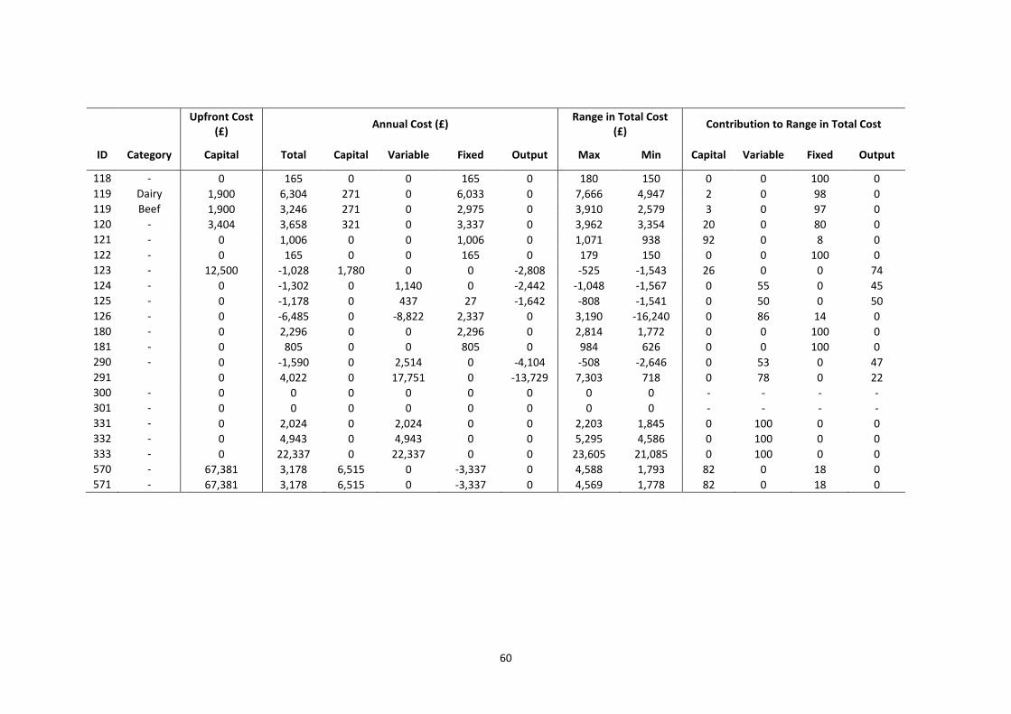
60
Upfront Cost
(£) Annual Cost (£)
Range in Total Cost
(£) Contribution to Range in Total Cost
ID Category Capital Total Capital Variable Fixed Output Max Min Capital Variable Fixed Output
118 - 0 165 0 0 165 0 180 150 0 0 100 0
119 Dairy 1,900 6,304 271 0 6,033 0 7,666 4,947 2 0 98 0
119 Beef 1,900 3,246 271 0 2,975 0 3,910 2,579 3 0 97 0
120 - 3,404 3,658 321 0 3,337 0 3,962 3,354 20 0 80 0
121 - 0 1,006 0 0 1,006 0 1,071 938 92 0 8 0
122 - 0 165 0 0 165 0 179 150 0 0 100 0
123 - 12,500 -1,028 1,780 0 0 -2,808 -525 -1,543 26 0 0 74
124 - 0 -1,302 0 1,140 0 -2,442 -1,048 -1,567 0 55 0 45
125 - 0 -1,178 0 437 27 -1,642 -808 -1,541 0 50 0 50
126 - 0 -6,485 0 -8,822 2,337 0 3,190 -16,240 0 86 14 0
180 - 0 2,296 0 0 2,296 0 2,814 1,772 0 0 100 0
181 - 0 805 0 0 805 0 984 626 0 0 100 0
290 - 0 -1,590 0 2,514 0 -4,104 -508 -2,646 0 53 0 47
291 0 4,022 0 17,751 0 -13,729 7,303 718 0 78 0 22
300 - 0 0 0 0 0 0 0 0 - - - -
301 - 0 0 0 0 0 0 0 0 - - - -
331 - 0 2,024 0 2,024 0 0 2,203 1,845 0 100 0 0
332 - 0 4,943 0 4,943 0 0 5,295 4,586 0 100 0 0
333 - 0 22,337 0 22,337 0 0 23,605 21,085 0 100 0 0
570 - 67,381 3,178 6,515 0 -3,337 0 4,588 1,793 82 0 18 0
571 - 67,381 3,178 6,515 0 -3,337 0 4,569 1,778 82 0 18 0

61
6.2.2 Variation in costs with time
The unit cost data within the Cost workbook contains a time series of data from 2000 to 2013, and is
updatable for future years. The user is able to select specific unit cost data either an individual year or
a range of years with which to calculate the mitigation method costs. The impacts of choosing two
different periods are shown in Figure 6-3. Unsurprisingly there is a linear trend in the dataset. The
costs of methods calculated using the more recent unit cost data are greater than those calculated
with the older data, but also the savings are also greater with the more recent data. There is some
scatter within the data, caused by some items in the unit costs data showing greater variation than
others, and also due to the time-series being complete for some data items and extrapolated for
others based upon an annual price change. It is also important to note that some mitigation methods
close to being cost neutral can switch from being a cost to a saving depending upon the data selected.
The two mitigation methods which have changed in the graph below are ‘Use manufactured fertiliser
placement technologies’, which is a cost in 2003-07, but a saving in 2008-12 and ‘Leave residual levels
of non-aggressive weeds’, which is a saving in 2003-07 and a cost in 2008-12. For fertiliser placement
technology, this difference is a result of the price of fertiliser increasing significantly over time (a 100%
increase between the two scenarios), whilst there is only a value for the GPS system for 2012 and the
tool simply extrapolates back in time using an annual price change (resulting in an 18% increase). Thus
there is now a bigger saving in fertiliser compared to the price of the system. Note that in reality, the
cost of a GPS system would probably be greater in the past as this new technology would have been
more expensive, and so this method would have been even more expensive in 2003-07 than the cost
predicted. For leaving residual weeds, the difference is because the arable output price has increased
significantly over time (by 63%), whilst the price of pesticides and pesticide applications has not
changed as much (17% and 35% respectively), thus the penalty of losing yield becomes more
significant over time.
-20,000
-10,000
0
10,000
20,000
-20,000 -10,000 0 10,000 20,000
Total Cost (£) - Average 2003 to 2007
Total Cost (£) - Average 2008-2012
Figure 6-3 Variation in the annual total costs of implementation resulting from different selections
of the data years to use for the unit costs. Values are for the default conglomerate farm within the
Cost workbook.

62
6.3 FIOs, Soil Carbon, Energy Use and Production
Farmscoper now predicts source apportioned baseline values for FIOs soil carbon, energy use and
production. The baseline values for four of the default farming systems within Farmscoper are shown
in Table 6-2. Emissions of FIOs are a function of the amount of livestock present, so there are no
losses on the mixed cereal farm (which has neither livestock nor manure). The highest FIO footprint is
on the dairy farm, but the indoor pig farm has a much lower value despite having a greater stocking
density. This is because all of the FIO losses on the pig farm are from managed manure (Table 6-3) and
the storage of the manure is of sufficient duration for a significant proportion of the FIO burden of the
manure to die-off before the manure is applied. For the dairy farm, the majority of the FIO loss comes
from excretion (voiding) as opposed to managed manure and so there is limited potential for die-off.
This is particularly true where livestock defecate directly in to water whilst grazing or travelling to and
from the yard. The soil carbon stocks are greatest on the pig farm and lowest on the dairy farm. This is
because the default soil carbon stocks per unit of grassland and arable land are comparable, so the
most important component of calculating the soil carbon stocks is the modifying factors taken from
the IPPC approach, with the highest factor used where arable land receives both manure and
fertiliser. The production values reflect the intensity of the system (i.e. stocking density for the
livestock farms), with highest values on the dairy and indoor pig farm and lowest values on the upland
cattle and sheep farm. Energy use is also related to the farm intensity, with the lowest values on the
upland cattle and sheep farm where there is limited machinery input (as there is limited rotational
land) and fertiliser rates are low. The apportionment of modelled farm energy use is shown in Table
6-4. The energy used in the production of fertilisers contributes between 55 and 65% of the total
energy use for the farms. On the arable farms, cultivating the land and storing the grain is a significant
source of energy use (approximately 20%). Housing livestock (particularly pigs and poultry) and
milking dairy animals also requiring significant energy.
Table 6-2 Summary results for the new pollutants and outcomes added to Farmscoper, for a
selection of default farming systems within Farmscoper. Values are for a 700-900mm climate and a
soil drained for arable fields (note that only FIO losses are affected by soil and climate).
Dairy Upland
Cattle &
Sheep
Indoor Pig &
Mixed
Cereal
Mixed
Cereal
Area
(ha) 114 146 197 197
Stocking Density
(kg N excreta ha-1) 162 61 176 -
FIOs
(109 cfu ha-1) 189 130 43 -
Soil Carbon
(t ha-1) 68 91 142 134
Energy Use
(kg CO2 ha-1) 1,655 294 1,977 1,708
Production
(£ ha-1) 2,667 378 2,288 1,104

63
Table 6-3 Losses of FIOs (109 cfu) for the selection of default farming systems, with apportionment
by source livestock and source type
Source
Livestock
Source
Type
Dairy Upland
Cattle &
Sheep
Indoor Pig &
Mixed
Cereal
Mixed
Cereal
Beef Dirty Water - 0 - -
Beef FYM 213 124 - -
Beef Slurry 1 - - -
Beef Voided 8754 7311 - -
Dairy Dirty Water 115 - - -
Dairy Slurry 517 - - -
Dairy Voided 10132 - - -
Pigs FYM - - 4149 -
Pigs Slurry - - 4387 -
Sheep FYM 2 13 - -
Sheep Voided 1737 11538 - -
Total - 21470 18986 8537 0
Table 6-4 Energy use (kg CO2) for the selection of default Farming systems, with apportionment by
source type.
Source Type Dairy Upland
Cattle &
Sheep
Indoor Pig &
Mixed
Cereal
Mixed
Cereal
Cultivation 4,044 379 42,459 42,459
Planting 499 35 4,081 4,081
Harvesting 10,882 7,120 11,811 11,811
Output 8,191 37,738 37,738
Fertiliser Production 106,763 26,187 217,850 217,850
Fertiliser Application 642 291 1,976 1,976
PPPs Production 835 122 18,210 18,210
PPPs Application 540 253 2,418 2,418
Housing 20,208 6,181 48,047 -
Milking 25,701 - - -
Cleaning 4,878 1,492 - -
Feeding 1,661 477 - -
FYM Application 358 498 3,110 -
Slurry Application 1,635 - 1,918 -
Dirty Water Application 1,044 4 - -

64
6.4 Upscaling
The Upscaling workbook allows Farmscoper to be applied at catchment to national scale. The
following results are from the tool being applied to the whole of England, to the 10 river basin
districts (RBDs) which cover England or to the 91 Water Management Catchments (WMCs) that cover
England.
6.4.1 Baseline Values
When applied to England and treating it as one area, the Upscaling workbook produces 171
Farmscoper Create files, reflecting the 10 different farm types on the 18 permutations of climate and
soil type (the 9 missing combinations are an LFA grazing farm in the climate zone with the lowest
rainfall and 8 combinations – mostly cereal and pig farms - in the climate zone with the highest
rainfall). The area weighted baseline values for the whole of England for this dataset are shown in
Table 6-5. The official IPCC inventory figures for agricultural emissions of methane and nitrous oxide
in 2010 are 10,008 and 18,901 kt CO2-e respectively (Thistlethwaite et al., 2012). Assuming a global
warming potential of 21 t CO2-e t-1 for methane and 310 CO2-e t-1 for nitrous oxide, the Farmscoper
totals are 9,718 kt CO2-e for methane (2% lower than the inventory total) and 21,461 kt CO2-e for
nitrous oxide (11% higher than the inventory total). There are a number of differences in the
management assumptions within Farmscoper that can explain these small differences. The national
inventory value for agricultural ammonia emissions in 2010 for England is 167 kt NH3 (MacCarty et al.,
2012). Using a factor of 1.22 to convert from NH3-N to NH3, the value predicted by Farmscoper for
England is 198 kt, (19% higher than the inventory total). Total agricultural production for the UK in
2010 was estimated as £14,151m, which is close to a figure of £15,363m for England in Defra et al.
(2012). The predicted energy use is 10,382 kt CO2, of which 3,961 kt comes from direct energy use
(i.e. not the embedded emissions associated with fertiliser and pesticide production). Warwick HRI &
FEC services (2007) estimated the direct energy use for the whole of UK agriculture was between
3,244 kt and 4,594 kt. Assuming that England contributes 75% of the UKs farm income (and thus
energy use), then a crude estimate of energy use in agriculture in England alone for comparison with
the Farmscoper figure is between 2,430 kt CO2 and 3,440 kt CO2.
Table 6-5 Baseline values for the pollutants and outcomes for the whole of England.
Pollutant Total Units for
Totals
Footprint Units for
Footprints
Nitrate 232 kt 27.6 kg ha-1
Phosphorus 4.52 kt 0.54 kg ha-1
Sediment 1,833 kt 218 kg ha-1
Ammonia 162 kt 19.3 kg ha-1
Methane 463 kt 54.9 kg ha-1
Nitrous Oxide 69 kt 8.2 kg ha-1
Pesticides 553,248 units 0.07 units ha-1
FIOs 653 1015 cfu 78 109 cfu ha-1
Soil Carbon 832 Mt 95.4 t ha-1
Energy Use 10,382 kt 1,233 kg ha-1
Production 14,151 £m 1,680 £ ha-1
The losses of nitrate, phosphorus and sediment as predicted by the Farmscoper Upscaling workbook
with WMC scale input data have been compared against results from the source models used to build
the Farmscoper coefficient database (i.e. NEAP-N and PSYCHIC) summarised to the same scale to
demonstrate that the two approaches remain comparable and thus Farmscoper is partly validated by
the validation of these source models. The results of these comparisons are shown in Figure 6-4.

65
There is a high correlation in the nitrogen loads (r2 = 0.92), with the majority of points close to the 1:1
line. The correlation is worse for phosphorus (r2 = 0.87) and sediment (r2 = 0.72), with more scatter
away from the 1:1 line. This is due to the strong dependence of sediment and phosphorus losses on
the soil type selected, due to the large contribution of losses in drain flow to total pollutant loads. The
soil type representation in PSYCHIC will be much more detailed than the three types within
Farmscoper, and the land use will be more spread out across the catchment that it is in Farmscoper
where it is all assigned to the location of the registered address for each farm holding.
This dependence of phosphorus and sediment emissions on soil type can also be seen in Table 6-6,
which shows the total results for England having run the Upscaling tool with the three different
spatial scales (England, RBD and WMC). The loads for most of the pollutants do not depend upon the
resolution of the input data, but there are noticeable differences for sediment, phosphorus and FIOs.
At these three different scales, the land will be allocated differently to the various farm types and
their associated soil and climate zones. For example, using the tool with England represented as one
big catchment, a crop may be allocated to a farm type that is found on each soil type. However, that
crop may only be found on that farm type in certain WMC catchments where the farms are mostly
found on only one soil type. Thus when running the tool at WMC scale, the crop will only be found on
certain soil types and so the pollutant loss from that crop type will be different.

66
0.0
2.0
4.0
6.0
8.0
10.0
0.0 2.0 4.0 6.0 8.0 10.0
Farmscoper Nitrogen Load (kt N)
NEAP-N Nitrogen Load (kt N)
0.00
0.05
0.10
0.15
0.20
0.25
0.00 0.05 0.10 0.15 0.20 0.25
Farmscoper Phosphorus Load (kt P)
PSYCHIC Phosphorus Load (kt P)
0
20
40
60
80
0 20 40 60 80
Farmscoper Sediment Load (kt S)
PSYCHIC Sedim
ent Load (kt S)
Figure 6-4 Comparison of agricultural nitrogen, phosphorus and sediment loads predicted by Farmscoper for the 91 Water Management Catchments in England against
loads predicted by the NEAP-N and PSYCHIC models for those same catchments. All model simulations used 2010 June Agricultural Census data.

67
Table 6-6 Comparison of the total values for England predicted by the Upscaling workbook using:
one catchment to represent the whole of England; the 10 RBDs in England; the 92 WMCs in England.
Pollutant Units England RBDs WMCs
Nitrate kt 232 227 227
Phosphorus kt 4.52 4.38 4.30
Sediment kt 1,833 1,692 1,625
Ammonia kt 162 163 163
Methane kt 463 464 464
Nitrous Oxide kt 69 69 69
Pesticides units 553,249 520,663 510,840
FIOs 1015 cfu 653 678 687
Soil Carbon Mt 832 836 829
Energy Use kt 10,382 10,418 10,433
Production £m 14,151 13,722 13,759
The Upscaling workbook includes graphical displays of the apportionment of pollutant emissions (and
outcomes) by catchment, farm type, climate zone and soil type, along with pollutant / outcome
footprints. Two screenshots of this are shown in Figure 6-5 (for nitrate) and Figure 6-6 (for sediment).
Emissions of nitrate are most intensive on the pig and poultry farms (58-76 kg ha-1) and even though
there are fewer of these than the other farm types (3,600 farms out of a total of 100,000 farms) they
are important in terms of a national apportionment by farm type. The lowland farm type is most
dominant (33,000 farms) but with a relatively small footprint does not contribute as much overall as
other farm types (i.e. cereals, dairy and general cropping). Losses of nitrate increase with increasing
annual average rainfall in the climate zones, except for in the wettest areas where the farms will be
less intensive and denitrification may be more likely. Losses of nitrate are greatest on the free-
draining soils. Conversely, sediment losses are greatest on the drained soils, where surface runoff is
higher and sediment is also transported through the drains. Losses of sediment increase with average
annual rainfall in the climate zones. Arable farms have the greatest sediment loads and contribute
over 50% of the total sediment budget.

68
Apportionment Footprint
kg kg ha-1
Summarised by farm type
Summarised by climate zone
Summarised by soil type
0 20 40 60 80 100
Cereals
General
Horticulture
Indoor Pig
Poultry
Dairy
LFA Grazing
Lowland Grazing
Mixed
Outdoor Pig
0 5 10 15 20 25 30 35
< 600 mm
600-700 mm
700-900 mm
900-1200 mm
1200-1500 mm
> 1500 mm
0 5 10 15 20 25 30 35
Free Draining
Drained - Arable
Drained - Arable
& Grass
Figure 6-5 Screenshot from the Upscaling workbook showing the apportionment of agricultural nitrate losses for England - in
the absence of mitigation method implementation - by farm type, climate zone and soil type.
69
Apportionment Footprint
kg kg ha-1
Summarised by farm type
Summarised by climate zone
Summarised by soil type
0 100 200 300 400 500
Cereals
General
Horticulture
Indoor Pig
Poultry
Dairy
LFA Grazing
Lowland Grazing
Mixed
Outdoor Pig
0 100 200 300 400
< 600 mm
600-700 mm
700-900 mm
900-1200 mm
1200-1500 mm
> 1500 mm
0 50 100 150 200 250 300 350
Free Draining
Drained - Arable
Drained - Arable
& Grass
Figure 6-6 Screenshot from the Upscaling workbook showing the apportionment of agricultural sediment losses for England - in
the absence of mitigation method implementation - by farm type, climate zone and soil type.

70
6.4.2 Impacts of mitigation
The Farmscoper mitigation method library contains over 100 methods, many of which are already
partially implemented on farms (or fully implemented on a proportion of farms). The impacts of this
prior implementation, and then a theoretical scenario assuming 100% implementation of all methods,
are shown in Table 6-7. The capital and operational costs of the prior implementation are roughly
equal in magnitude, except the operational costs are actually a saving, mostly through reduced inputs
(i.e. fertiliser), such that the total cost of prior implementation is effectively zero. The largest
reductions in pollutant loads (with respect to the baseline values) are for pesticides and FIOs at over
20%, the phosphorus reduction is almost 13% and the other pollutants are reduced by under 10%.
Energy use is reduced by 4%, and there is a 1% reduction in the amount of production. The
environmental benefit of this prior implementation is £247m. The impacts of maximum
implementation (with respect to the prior situation) are reductions in pollutant loads of up to 38%,
with methane the smallest reduction at 14%. These are associated with a 27% reduction in energy use
and an 8% reduction in production. The total cost of implementation is £1,390m, with an
environmental benefit of £659m. Note that the total impact of the mitigation methods on soil carbon
are negligible (discussed below).
The prior implementation and competition rules within Farmscoper can constrain the magnitude of
the reductions that can be predicted. For competition, this is because the default choice of method
implemented where two or more are mutually exclusive is often set to be the one most likely to be
implemented by a farmer rather than the one most likely to achieve the best pollutant reductions
(e.g. just leaving stubbles over winter as opposed to planting a purpose grown cover crop). It is also
important to note that Farmscoper assumes that once a method has been implemented as part of the
prior implementation scenario, it cannot be replaced by a different method where they are in
competition.
Table 6-7 Impacts of mitigation method implementation for the whole of England. Values with prior
implementation rates as specified in Table 5-3 differenced from the baseline values, and values
with 100% implementation of mitigation methods differenced from the prior situation.
Change from Baseline to
Prior Implementation
Change from Prior to
Maximum Implementation
Capital Cost (£m) 136 944
Operational Cost (£m) -130 446
Total Cost (£m) 6 1,390
Environmental Benefit (£m) 247 659
Nitrate (%) 8.9 19.4
Phosphorus (%) 8.5 31.3
Sediment (%) 6.8 28.5
Ammonia (%) 6.3 29.2
Methane (%) 2.5 14.3
Nitrous Oxide (%) 6.9 18.8
Pesticides (%) 22.5 38.5
FIOs (%) 14.0 21.7
Soil Carbon (%) 0.0 0.1
Energy Use (%) 3.7 27.3
Production (%) 1.3 7.5

71
The Upscaling workbook can also determine the impacts of mitigation methods applied individually.
The results of doing this for the whole of England, using every method in the Farmscoper method
library, are shown in Table 6-8. Note that these values are expressed relative to the prior
implementation values, so some methods appear to have a low effect because they are already
implemented across much of the land (see Table 5-3 for the prior implementation rates used). The
value from totalling the nitrate reductions for all methods is 28% - if this is compared to the value of
19% shown in Table 6-7, it gives an idea of the reductions ‘lost’ through method interactions (i.e.
diminishing returns where multiple methods target the same sources and due to competition
between mutually exclusive methods). The results in Table 6-8 are summarised in Table 6-9, which
shows the top five mitigation methods for reducing each pollutant, stating the reduction achieved,
cost of implementation, environmental benefit and any impact on production. ‘Uncropped cultivated
areas’ is one of the key methods for nitrate, phosphorus and sediment reduction in this table. This is
because it involves taking large areas of land out of production (approximately 1 ha per field), but
then consequently having the highest cost of all methods and the largest impact on production of all
methods. ‘Plant areas of farm with wild bird seed / nectar flower mixtures’ also achieves high
reductions but at a cost, as it involves taking large areas out of production. The probability of either of
these methods being applied across all agricultural land is minimal, whereas other methods within
Farmscoper should achieve high levels of implementation because they correspond closely to
agricultural policy regulations (e.g. the NVZ action programme). ‘Extend the grazing season for cattle’
is a method that reduces ammonia emissions and also results in cost savings. The opposite method -
‘Reduce the length of the grazing season’ - achieves the highest level of nitrous oxide reductions. The
environmental benefit of both methods is comparable. ‘Anaerobic digestion of livestock manures’
reduces methane emissions by 11% and is also one of the top methods for reducing FIO emissions.
The method results in a net cost saving (due to payment rates assumed for the electricity generated)
and is assumed to have no impacts on production. This second point is a consequence of applying a
farm scale tool at national scale – a single farm could import the necessary feedstock to run the
digester from neighbouring farms without impacting on its own production levels, but at a national
scale, the use of land for feedstock on neighbouring farms would impact on the national level of
production (the choice of assuming feedstock is imported on to the farm is made because of how
Farmscoper is not able to represent system level changes as mitigation methods, with an unknown
amount of land use change required, as well as potential changes in livestock numbers assuming the
land once used for forage is now used for feedstock).

72
Table 6-8 Costs and impacts (percentage change) for each mitigation method in Farmscoper, expressed relative to the prior implementation. A negative cost is a saving,
a negative percentage change is an increase. Values are for the whole of England. Please refer to Table 5-3 for Method Names, which are linked to Method IDs.
ID
Ca
pit
al
Co
st
(£m
)
Op
era
tio
na
l C
ost
(£m
)
To
tal
Co
st
(£m
)
En
vir
on
me
nta
l
Be
ne
fit
(£m
)
Nit
rate
(%)
Ph
osp
ho
rus
(%)
Se
dim
en
t
(%)
Am
mo
nia
(%)
Me
tha
ne
(%)
Nit
rou
s O
xid
e
(%)
Pe
stic
ide
s
(%)
FIO
s
(%)
So
il C
arb
on
(%)
En
erg
y U
se
(%)
Pro
du
ctio
n
(%)
4 0 42 42 108 3.7 6.7 13.1 0.0 0.0 0.5 0.4 0.1 0.0 -0.4 0.0
5 0 40 40 13 0.4 0.8 1.6 0.0 0.0 0.0 0.0 0.0 0.0 0.0 0.0
6 0 170 170 16 0.7 2.1 1.6 0.0 0.0 0.1 0.1 0.0 0.0 -0.1 1.7
7 0 -45 -45 36 1.6 0.9 2.4 0.0 0.0 0.6 -2.1 0.0 0.0 1.1 0.0
8 0 37 37 28 0.4 1.6 3.3 0.0 0.0 0.5 2.1 0.1 0.0 -0.6 0.0
9 0 8 8 18 0.3 0.9 2.2 0.0 0.0 0.0 1.9 0.1 0.0 0.0 0.0
10 0 30 30 247 0.0 0.0 0.0 0.0 0.0 0.0 -0.2 0.0 0.0 -0.1 0.0
11 0 1 1 2 0.1 0.1 0.3 0.0 0.0 0.0 0.9 0.0 0.0 0.0 0.0
13 1 24 25 26 0.1 1.5 3.6 0.0 0.0 0.0 0.7 0.1 0.0 0.0 0.0
14 5 43 47 54 0.8 2.5 5.3 0.4 0.0 0.5 6.3 0.1 0.0 0.8 0.6
15 0 52 52 30 0.4 2.2 2.0 0.0 0.0 0.9 0.0 0.3 0.0 0.0 0.0
16 0 82 82 -18 0.2 0.6 0.3 0.0 0.0 -1.6 0.0 0.0 0.0 -0.2 0.0
19 0 -240 -240 20 0.2 0.4 0.0 0.9 1.7 0.4 0.0 0.0 0.0 0.0 -0.7
20 0 -52 -52 78 2.9 0.0 0.0 3.3 0.0 2.5 0.0 0.0 0.0 3.9 0.0
21 0 -25 -25 0 0.1 0.0 0.0 0.0 0.0 0.0 0.0 0.0 0.0 0.0 0.3
22 0 -7 -7 5 0.3 0.0 0.0 0.2 0.0 0.2 0.0 0.0 0.0 0.0 0.0
23 0 -138 -138 10 0.5 0.5 0.0 0.4 0.0 0.4 0.0 0.0 0.0 0.3 0.0
25 0 16 16 4 0.1 0.0 0.0 0.2 0.0 0.1 0.0 0.0 0.0 0.2 0.1
26 0 134 134 6 0.2 1.5 0.0 0.7 0.0 0.0 0.0 0.0 0.0 0.0 0.9
27 23 -42 -20 27 0.4 0.1 0.0 0.5 0.0 0.1 0.0 0.0 0.0 3.6 0.0
28 0 16 16 4 1.0 0.0 0.0 0.0 0.0 0.1 0.0 0.0 0.0 0.0 0.0
31 0 -197 -197 66 0.6 0.0 0.0 0.4 0.0 0.6 0.0 0.0 0.0 8.6 0.0
32 0 -24 -24 6 0.0 1.0 0.0 0.0 0.0 0.0 0.0 0.0 0.0 0.7 0.0
34 1 -4 -3 1 0.1 0.0 0.0 0.1 0.0 0.0 0.0 0.0 0.0 0.0 0.0

73
ID
Ca
pit
al
Co
st
(£m
)
Op
era
tio
na
l C
ost
(£m
)
To
tal
Co
st
(£m
)
En
vir
on
me
nta
l
Be
ne
fit
(£m
)
Nit
rate
(%)
Ph
osp
ho
rus
(%)
Se
dim
en
t
(%)
Am
mo
nia
(%)
Me
tha
ne
(%)
Nit
rou
s O
xid
e
(%)
Pe
stic
ide
s
(%)
FIO
s
(%)
So
il C
arb
on
(%)
En
erg
y U
se
(%)
Pro
du
ctio
n
(%)
35 0 96 96 6 0.1 1.0 2.0 -8.9 -2.6 3.7 0.0 1.6 0.0 -0.5 0.0
36 0 -96 -96 2 -0.1 -1.0 -0.8 8.9 2.6 -3.7 0.0 -1.6 0.0 0.5 0.0
37 0 96 96 0 0.1 0.5 0.5 -1.9 -0.6 0.6 0.0 0.4 0.0 -0.1 0.0
38 0 24 24 11 0.1 0.3 0.5 0.0 0.0 0.5 0.0 1.6 0.0 0.0 0.0
39 8 0 8 11 0.1 0.3 0.5 0.0 0.0 0.5 0.0 1.6 0.0 0.0 0.0
42 0 63 63 10 0.0 0.0 0.0 2.7 0.0 0.0 0.0 0.0 0.0 -0.2 0.0
43 0 85 85 11 0.0 0.0 0.0 2.6 0.0 0.0 0.0 0.0 0.0 0.0 0.0
44 0 53 53 6 0.0 0.0 0.0 1.4 0.0 0.0 0.0 0.0 0.0 0.0 0.0
46 4 0 4 2 0.0 0.0 0.0 0.4 0.0 0.0 0.0 0.0 0.0 0.0 0.0
48 41 26 67 4 0.0 0.0 0.0 1.0 0.0 0.0 0.0 0.0 0.0 -0.1 0.0
50 0 0 0 0 0.0 0.0 0.0 0.1 0.0 0.0 0.0 0.0 0.0 0.0 0.0
51 0 4 4 1 0.0 0.0 0.0 0.2 0.0 0.0 0.0 0.0 0.0 -0.1 0.0
52 47 0 47 1 0.2 0.7 0.0 -0.3 0.0 0.0 0.0 1.7 0.0 0.0 0.0
53 77 0 77 -1 0.0 0.0 0.0 -0.3 0.0 0.0 0.0 2.7 0.0 0.0 0.0
54 83 -13 71 0 0.0 0.0 0.0 0.0 0.0 0.0 0.0 0.0 0.0 0.1 0.0
55 1 2 3 4 0.0 0.0 0.0 0.0 0.7 0.0 0.0 0.0 0.0 0.0 0.0
56 455 -792 -336 101 0.0 0.0 0.0 -0.3 11.1 0.0 0.0 3.6 0.0 5.4 0.0
59 0 8 8 18 0.0 0.0 0.0 4.2 0.0 0.0 0.0 2.7 0.0 0.0 0.0
60 0 0 0 0 0.0 0.1 0.0 0.0 0.0 0.0 0.0 0.2 0.0 0.0 0.0
61 20 8 28 2 0.1 0.9 0.0 0.0 0.0 0.0 0.0 1.6 0.0 0.0 0.0
62 3 0 4 -4 0.0 0.2 0.0 -1.1 0.0 0.0 0.0 0.8 0.0 0.0 0.0
63 38 1 39 1 0.0 0.1 0.0 0.2 0.0 0.0 0.0 0.1 0.0 0.0 0.0
64 0 2 2 9 0.0 0.1 0.0 2.1 0.0 0.0 0.0 0.0 0.0 0.0 0.0
67 0 1 1 1 0.3 0.0 0.0 0.0 0.0 0.0 0.0 0.0 0.0 0.0 0.0
68 0 0 0 0 0.0 0.0 0.0 0.0 0.0 0.0 0.0 0.0 0.0 0.0 0.0
69 0 0 0 20 0.4 2.0 0.0 0.0 0.0 1.3 0.0 1.1 0.0 0.0 0.0
70 0 26 26 14 -0.7 0.0 0.0 4.2 0.0 -0.1 0.0 0.0 0.0 -0.1 0.0

74
ID
Ca
pit
al
Co
st
(£m
)
Op
era
tio
na
l C
ost
(£m
)
To
tal
Co
st
(£m
)
En
vir
on
me
nta
l
Be
ne
fit
(£m
)
Nit
rate
(%)
Ph
osp
ho
rus
(%)
Se
dim
en
t
(%)
Am
mo
nia
(%)
Me
tha
ne
(%)
Nit
rou
s O
xid
e
(%)
Pe
stic
ide
s
(%)
FIO
s
(%)
So
il C
arb
on
(%)
En
erg
y U
se
(%)
Pro
du
ctio
n
(%)
71 0 13 13 34 0.6 3.6 0.0 6.8 0.0 0.1 0.0 1.4 0.0 -0.3 0.0
72 0 0 0 14 0.3 1.2 0.0 0.0 0.0 0.9 0.0 0.1 0.0 0.0 0.0
73 0 28 28 7 0.2 0.4 0.0 1.5 0.0 0.0 0.0 0.8 0.0 -0.2 0.0
76 87 7 95 3 0.2 1.6 0.0 0.0 0.0 0.0 0.0 7.4 0.0 0.0 0.0
77 3 0 3 0 0.0 0.2 0.0 0.0 0.0 0.0 0.0 0.5 0.0 0.0 0.0
78 7 16 23 19 0.3 1.6 2.3 0.0 0.0 0.0 0.0 0.0 0.0 0.0 0.0
79 2 0 2 0 0.0 0.0 0.0 0.0 0.0 0.0 0.0 0.0 0.0 0.0 0.0
80 48 1 49 0 0.0 0.0 0.0 0.0 0.0 0.0 0.0 0.0 0.0 0.0 0.0
81 36 3 39 1 0.1 0.5 0.0 0.0 0.0 0.0 0.0 1.5 0.0 0.0 0.0
82 43 -175 -132 0 0.2 0.0 0.0 0.0 0.0 0.0 0.0 0.0 0.0 -0.1 -0.9
83 1 3 4 0 0.0 0.0 0.0 0.1 0.0 0.0 0.0 0.0 0.0 0.0 0.0
90 0 0 0 0 0.0 0.0 0.0 0.0 0.0 0.0 0.2 0.0 0.0 0.0 0.0
91 0 -46 -46 1 0.0 0.0 0.0 0.0 0.0 0.0 11.8 0.0 0.0 0.1 0.0
92 0 67 67 0 0.0 0.0 0.0 0.0 0.0 0.0 5.3 0.0 0.0 0.0 0.6
94 0 1 1 0 0.0 0.0 0.0 0.0 0.0 0.0 2.6 0.0 0.0 0.0 0.0
95 0 2 2 0 0.0 0.0 0.0 0.0 0.0 0.0 1.2 0.0 0.0 0.0 0.0
96 4 0 4 0 0.0 0.0 0.0 0.0 0.0 0.0 11.8 0.0 0.0 0.0 0.0
97 3 0 3 0 0.0 0.0 0.0 0.0 0.0 0.0 2.8 0.0 0.0 0.0 0.0
101 0 0 0 0 0.0 0.0 0.0 0.0 0.0 0.0 0.0 0.0 0.0 0.0 0.0
102 0 8 8 1 0.1 0.0 0.1 0.0 0.0 0.0 0.0 0.0 0.0 0.1 0.0
103 1 1 2 1 0.0 0.1 0.1 0.0 0.0 0.0 0.0 0.3 0.0 0.0 0.0
105 0 57 57 12 0.1 0.6 1.4 0.0 0.0 0.0 0.5 0.0 0.0 0.2 0.8
106 18 195 213 58 1.1 2.4 4.6 0.6 0.0 0.8 1.2 0.0 0.0 1.3 0.8
107 5 198 202 11 0.1 0.6 1.4 0.0 0.0 0.0 0.5 0.0 0.0 0.0 0.0
108 0 32 32 32 1.1 0.9 1.4 0.1 0.0 0.8 1.0 0.0 0.0 1.3 0.9
109 0 14 14 0 0.0 0.0 0.0 0.0 0.0 0.0 0.0 0.0 0.0 0.0 0.0
110 0 397 397 164 5.3 4.6 7.2 2.8 0.0 3.4 4.9 0.0 0.0 6.4 4.4

75
ID
Ca
pit
al
Co
st
(£m
)
Op
era
tio
na
l C
ost
(£m
)
To
tal
Co
st
(£m
)
En
vir
on
me
nta
l
Be
ne
fit
(£m
)
Nit
rate
(%)
Ph
osp
ho
rus
(%)
Se
dim
en
t
(%)
Am
mo
nia
(%)
Me
tha
ne
(%)
Nit
rou
s O
xid
e
(%)
Pe
stic
ide
s
(%)
FIO
s
(%)
So
il C
arb
on
(%)
En
erg
y U
se
(%)
Pro
du
ctio
n
(%)
111 0 174 174 15 0.3 0.1 0.8 0.0 0.0 0.3 0.6 0.0 0.0 0.7 0.4
112 0 121 121 21 0.3 0.3 1.3 0.4 0.0 0.4 0.6 0.0 0.0 0.7 0.4
113 0 -4 -4 29 1.1 1.8 3.3 0.0 0.0 0.1 0.1 0.0 0.0 0.0 0.2
114 0 209 209 16 0.2 0.5 0.5 0.1 0.0 0.7 0.0 0.0 0.0 0.4 0.0
115 0 38 38 16 0.7 2.1 1.6 0.0 0.0 0.1 0.1 0.0 0.0 -0.1 0.0
116 0 15 15 3 0.0 0.0 0.0 0.0 0.0 0.0 4.9 0.0 0.0 0.5 0.9
117 -4 -69 -73 11 0.1 0.4 1.0 0.0 0.0 0.0 1.5 0.0 0.0 0.4 0.0
118 0 1 1 8 0.0 0.2 0.2 0.0 0.0 0.5 0.0 0.5 0.0 0.0 0.0
119 10 150 160 0 0.2 0.6 0.0 0.0 0.0 0.0 0.0 1.9 0.0 -0.3 0.0
120 1 6 6 1 0.2 0.5 0.0 0.0 0.0 0.0 0.0 1.6 0.0 0.0 0.0
121 0 6 6 0 0.0 0.0 0.0 0.0 0.0 0.0 0.0 0.0 0.0 0.0 0.0
122 0 1 1 0 0.0 0.0 0.0 0.0 0.0 0.0 0.0 0.0 0.0 0.0 0.0
123 13 -21 -8 1 0.0 0.0 0.0 0.0 0.0 0.0 0.0 0.0 0.0 0.0 -0.2
124 0 -2 -2 9 0.0 0.0 0.0 0.0 1.5 0.0 0.0 0.0 0.0 0.0 -0.5
125 0 -48 -48 0 0.1 0.0 0.0 0.0 0.0 0.0 0.0 0.0 0.0 0.0 0.0
126 0 -6 -6 0 0.0 0.0 0.0 0.0 0.1 0.0 0.0 0.0 0.0 0.0 0.0
180 0 10 10 -3 -0.3 -0.4 -0.6 0.0 0.0 0.2 -0.2 0.0 0.0 0.0 0.0
181 0 9 9 1 -0.1 -0.5 -0.2 0.0 0.0 0.3 0.0 0.0 0.0 0.0 0.0
290 0 -5 -5 -3 0.0 0.0 0.0 0.2 0.0 0.0 0.0 0.0 0.0 -0.6 0.0
291 0 19 19 -42 0.0 0.0 0.0 6.3 0.0 0.0 0.0 0.0 0.0 -10.7 -0.2
300 0 0 0 1 0.0 0.0 0.0 0.1 0.0 0.0 0.0 0.0 0.0 0.0 0.0
301 0 0 0 17 0.0 0.0 0.0 3.9 0.0 0.0 0.0 0.0 0.0 0.0 0.0
331 0 21 21 9 0.2 0.2 0.0 0.4 0.7 0.1 0.0 0.0 0.0 0.0 0.0
332 0 2 2 1 0.1 0.0 0.0 0.2 0.0 0.0 0.0 0.0 0.0 0.0 0.0
333 0 5 5 2 0.2 0.0 0.0 0.3 0.0 0.0 0.0 0.0 0.0 0.0 0.0
570 4 -2 2 0 0.0 0.0 0.0 0.0 0.0 0.0 0.0 0.0 0.0 0.0 0.0
571 7 -2 5 0 0.0 0.0 0.0 0.0 0.0 0.0 0.0 0.0 0.0 0.0 0.0

76
Table 6-9 Top five mitigation methods for pollutant reductions when implemented across all of
England, determined for each individual pollutant, along with implementation costs, overall
environmental benefits and impacts on production (summarised from Table 6-8).
Mitigation Method
Reduction
(%)
Total
Cost
(£m)
Environ.
Benefit
(£m)
Production
Impact
(£m)
Nitrate
Uncropped cultivated areas 5.3 397 164 4.4
Establish cover crops in the autumn 3.7 42 108 0.0
Use plants with improved nitrogen use efficiency 2.9 -52 78 0.0
Adopt reduced cultivation systems 1.6 -45 36 0.0
Plant areas of farm with wild bird seed / nectar flower mixtures 1.1 213 58 0.8
Phosphorus
Establish cover crops in the autumn 6.7 42 108 0.0
Uncropped cultivated areas 4.6 397 164 4.4
Use slurry injection application techniques 3.6 13 34 0.0
Establish riparian buffer strips 2.5 47 54 0.6
Plant areas of farm with wild bird seed / nectar flower mixtures 2.4 213 58 0.8
Sediment
Establish cover crops in the autumn 13.1 42 108 0.0
Uncropped cultivated areas 7.2 397 164 4.4
Establish riparian buffer strips 5.3 47 54 0.6
Plant areas of farm with wild bird seed / nectar flower mixtures 4.6 213 58 0.8
Establish in-field grass buffer strips 3.6 25 26 0.0
Ammonia
Extend the grazing season for cattle 8.9 -96 2 0.0
Use slurry injection application techniques 6.8 13 34 0.0
Replace urea fertiliser to arable land with another form 6.3 19 -42 -0.2
Compost solid manure 4.2 8 18 0.0
Use slurry band spreading application techniques 4.2 26 14 0.0
Methane
Anaerobic digestion of livestock manures 11.1 -567 101 0.0
Extend the grazing season for cattle 2.6 -96 2 0.0
Make use of improved genetic resources in livestock 1.7 -240 20 -0.7
Use high sugar grasses 1.5 -2 9 -0.5
Reduce dietary N and P intakes: Dairy 0.7 21 9 0.0
Nitrous Oxide
Reduce the length of the grazing day/grazing season 3.7 96 6 0.0
Uncropped cultivated areas 3.4 397 164 4.4
Use plants with improved nitrogen use efficiency 2.5 -52 78 0.0
Do not spread slurry or poultry manure at high-risk times 1.3 0 20 0.0
Loosen compacted soil layers in grassland fields 0.9 52 30 0.0
Pesticides
Construct bunded impermeable PPP filling/mixing/cleaning area 11.8 -46 1 0.0
Fill/Mix/Clean sprayer in field 11.8 4 0 0.0
Establish riparian buffer strips 6.3 47 54 0.6
Avoid PPP application at high risk timings 5.3 67 0 0.6
Uncropped cultivated areas 4.9 397 164 4.4
FIOs
Fence off rivers and streams from livestock 7.4 95 3 0.0
Anaerobic digestion of livestock manures 3.6 -567 101 0.0
Adopt batch storage of slurry 2.7 77 -1 0.0
Compost solid manure 2.7 8 18 0.0
Use dry-cleaning techniques to remove solid waste from yards 1.9 160 0 0.0

77
7 Discussion and Conclusions
The previous version of the Farmscoper tool has been used by a variety of government organisations,
research institutes, consultancies, levy bodies and other agricultural organisations for more complex
assessments of the impacts of policy scenarios and agri-environment schemes through to prioritising
catchment management plans and assessing pollutant footprints and mitigation potential of
individual farms or groups of farms. The Farmscoper webpage on the ADAS website from which the
tool can be downloaded has had almost 3,000 unique page views since it was created in 2012.
This project funded the expansion or development of Farmscoper in four areas:
1. The addition of more pollutants (FIOs and carbon from energy use) and outcomes (soil
carbon stocks and production)
2. A review of prior implementation rates
3. A new Cost workbook
4. A new Upscaling workbook
The calculation of carbon from energy use replaces the energy use indicator in the previous version of
Farmscoper (where there was only a qualitative assessment of the impacts of mitigation
implementation). The inclusion of a calculated baseline farm energy use provides a more complete
assessment of carbon footprints and a more robust assessment of potential GHG mitigation. It also
helps to identify win-win scenarios where there is a quantifiable benefit to the farmer in terms of
reduced expenditure on fuel. Source apportioned emissions of carbon from energy use were
calculated for all major farming operations, as well as the embedded emissions from fertiliser and
pesticide production. The embedded emissions typically account for around 60% of the energy use,
with land management (cultivation, planting and harvesting) and housing livestock the other major
sources of energy use. Farmscoper predicts that large savings in energy use can be made (27%
reduction if all 105 mitigation methods are implemented), but this is mostly because of reductions in
embedded emissions associated with reduced fertiliser use.
The inclusion of FIOs within Farmscoper will provide an additional benefit when the tool is applied in
areas where bathing water quality and shellfish production are important. The majority of FIO losses
are associated with direct deposition of excreta in watercourses, unlike with manure or excreta
deposited in fields where faecal die-off can significantly reduce the concentrations of FIOs in runoff
and drain flow. On dairy farms where livestock cross watercourses on the way to and from the milking
parlour and grazing fields are not fenced off from streams, the direct deposition contribution can be
over 80% of the total load. Thus mitigating this, through fencing and the construction of bridges, is the
most successful approach to reducing FIO losses.
Farmscoper now estimates the production of the farm system, using output prices per head of
livestock or per hectare of cropping (accounting for forage used on farm). This source apportioned
production value allows for the impacts of mitigation method implementation on production to be
calculated exactly as per the pollutant emissions, i.e. through a percentage change in the value from a
set of coordinates (e.g. buffer strips results in a 2% reduction in arable outputs). This allows for
production to be explicitly considered when evaluating mitigation scenarios, as well as it being
accounted for as part of the cost of implementation.
The tool now also calculates soil carbon stocks, following an enhanced IPCC inventory Tier 1 approach.
Due to the carbon stock values for arable land and grassland not being that different, the impacts of
mitigation method implementation on carbon stocks are limited. However, the tool can be used to
determine the impacts of system level changes (i.e. reversion to grassland or increased area of
woodland), at both farm and – using the upscaling tool – catchment to national scale.
Farmscoper also now qualitatively estimates the impacts of mitigation implementation on soil quality,
scoring the impacts of the mitigation methods on soil water holding capacity, aeration and drainage.
Farmscoper allows the user to specify the implementation rates of the different mitigation methods
prior to the scenario being investigated. The original version of Farmscoper was populated with prior
implementation rates for all mitigation methods, to reflect national average rates. These prior

78
implementation rates have been reviewed as part of this project, using the available evidence base
from national stratified surveys of farm practice. The justification for the prior implementation rates
for each mitigation method is included in this report, and Farmscoper has now been modified to allow
the user to edit and alter the rates. It should be noted that the prior implementation rates are
average rates reflecting national trends, and will not be representative of any one particular farm.
This is particularly true of mitigation methods that are either implemented or not at a farm scale, but
where a proportion of farms may have done so (e.g. slurry store covers), as opposed to those where
partial implementation is more possible at farm scale (e.g. avoid high risk areas). Thus, for an
individual farm, the default prior implementation rates should be used with caution.
One of the key developments in the revised Farmscoper is the new Cost workbook. The previous cost
data within Farmscoper was somewhat opaque, not readily auditable and reflected a range of
different assumptions and time periods. By creating a separate workbook which lays out all the cost
components and the assumptions used in the costing up of the mitigation methods as well as
ensuring, where possible, that mitigation methods use a uniform set of data and assumptions, the
intention is to make the cost element of Farmscoper more robust and auditable. This is particularly
important as the cost data is often the part of the tool that users are more familiar with and able to
question. This Cost workbook has been designed to operate as a stand alone tool so that users can
assess the costs of different mitigation methods, assumptions, input data etc without the need to use
the other Farmscoper workbooks.
Although Farmscoper was designed to quantify pollutant losses and mitigation impacts at a farm
scale, users have applied - or tried to apply – the previous version to catchments or other spatial units
by representing them as a number of different farms or simply one mega-farm (i.e. all land use and
livestock in a catchment put in as one farm). The development of the Upscaling workbook allows
users to automate the generation of multiple farms and calculation of their pollutant impacts, and
then to take these results forward for assessments of mitigation potential. The automation allows for
a more stream-lined approach which is significantly faster than ‘hand-worked’ attempts by both users
and the developers of Farmscoper to derive catchment level impacts.
As a demonstration of the capability of the upscaling tool, pollutant emissions were generated for the
whole of England using agricultural data at a range of scales. The choice of scale (England as one
catchment down to 100 water management catchments), made little impact on most total pollutant
emissions. However, for phosphorus and sediment emissions, the change in scale changed total
emissions by 5 and 12% respectively. This is because the presence of under drainage significantly
increases phosphorus and sediment emissions, and with the coarser data, more land ended up
attributed to the farm types found on the soils with drainage. National total emission for methane
and nitrous oxide were comparable to the official inventory values, which use similar calculations, but
different assumptions. Results for nitrate, phosphorus and sediment are comparable to the source
models upon which they were based, which was the intention of area-weighting the pollutant loss
coefficients across the soil and climate zones within England and Wales. Using the revised
assumptions of prior implementation rates, the tool predicted that prior implementation of mitigation
methods in England reduced nitrate, phosphorus, sediment, ammonia and nitrous oxide emissions by
between 6 and 9%, with comparatively little cost to the farming sector (£6m per annum). Applying the
full set of 105 mitigation methods in Farmscoper on top of this resulted in additional reductions of
most pollutants of 15 to 40%. These extra reductions would be at a cost of £1,160m, with a potential
7% reduction in agricultural production. More realistic results than this demonstration scenario could
be found by either applying more realistic national implementation scenarios, or only focussing on
catchments where specific pollutants are an issue and selecting methods appropriately.
There are a few consequences of applying the Farmscoper tool nationwide (which may apply to other
cost-effect of mitigation models/frameworks). Firstly, a number of the mitigation methods assume
other material (e.g. additional straw or forage, of feedstock for an anaerobic digester) are grown off-
farm and can be bought in. Whilst this may be a legitimate assumption at farm or small catchment
scale, at a national scale this would require materials to be bought in from other countries or
additional consequences on production and pollutant emissions within this country not accounted for
within this tool (e.g. more land devoted to maize production). There is also the possibility that
widespread implementation of certain mitigation methods could alter the supply and demand for raw
materials or additional suppliers could increase competition in the market place.

79
7.1 Future work
Significant effort has gone in to providing help within the Farmscoper workbooks and producing
supporting documentation on how to use the tool and the background behind the different
components, and Farmscoper has now inevitably become more complex as more functionality and
scope has been added. Feedback from government and NGO users is that training is required to
enable users to get the most out of Farmscoper, and this would also help to ensure that any
conclusions drawn from using Farmscoper reflect the methodology applied with Farmscoper and the
assumptions and limitations of the tool. This training material would include case studies of
Farmscoper being applied for different purposes.
The Farmscoper tool has been widely used by a variety of organisations, at different scales and for
different purposes. It would be useful to hold a conference at which users of Farmscoper could
discuss the work they have undertaken with the tool, say how outputs have been disseminated to the
farming community, reveal the lessons they have learn through applying Farmscoper and share any
modifications or amendments to the Farmscoper mitigation method library. This would also provide a
forum to discuss potential future application and development of the tool.
The review of prior implementation data was based upon the best available nationally survey data on
agricultural practice. As has been stated earlier, these data can reflect the proportion of farms
undertaking an activity, where that activity can only be done or not done at farm scale, or may not
reflect what is happening in smaller catchments. Therefore it would be beneficial to determine at
what spatial scale the prior implementation data become appropriate, given the uncertainty in
applying national data at smaller scales. We would statically model the uncertainty arising in the
downscaling on national data on the uptake of mitigation methods and the underlying assumptions in
the derivation of the smart pollutant loss export coefficients (e.g. fertiliser timing), taking account of
the number and mix of farm types present at a range of spatial scales. This would provide critical
information on whether changes in pollutant pressure calculated at catchment scale are robust, i.e.
insensitive to uncertainties in the input agricultural census data.
The mitigation method library now contains 105 methods. The tool was originally designed - and
retains the capability - for a user to adjust or add new mitigation methods to this library. However,
now that this involves the specification of the impacts of a mitigation method on up to 14 different
pollutants or outcomes, as well as a detailed cost calculation, it is unlikely that users will add new
methods. There are number of potential mitigation methods to include within Farmscoper, such as
some of those identified in the Defra ‘Basic Measures’ Project (Newell-Price et al, 2014), although it
must be remembered that Farmscoper cannot easily represent mitigation methods requiring large
scale system change, and there is not sufficient evidence to differentiate between some methods that
may at first appear different (e.g. different widths of buffer strip). There is also the need to maintain
an ongoing review of new data as it arises, especially those from detailed meta-analysis of existing
data. The Farmscoper Cost workbook has been populated with unit cost data for 2000 to 2013. It is
advisable that a regular update of the Cost workbook is maintained.
The user is able to modify the pollutant losses generated with Farmscoper, or even over-write them
entirely if, for example, they feel that an alternative model is more appropriate for representing the
pollutant losses occurring within a specific area. They can then use the rest of the Farmscoper
framework to calculate the cost-effectiveness of mitigation method implementation on those revised
/ alternate pollutant losses. However, currently no one has undertaken this procedure, possibly either
due to a lack of awareness of this functionality or due to uncertainty about how to implement it.
Therefore it would be useful if this procedure could be demonstrated, together with the creation of a
protocol or additional interface to allow users to transform model outputs into the terminology
required by Farmscoper. The demonstration of this procedure would show the sensitivity of
Farmscoper outputs, at farm scale, to the choice of input model.
There are a number of record keeping / management systems (e.g. PLANET, GateKeeper) that require
farmers to specify a range of crop and livestock management data, and which already have significant
uptake within the farming community. A mechanism for automatically populating the Farmscoper
input data from these existing datasets may encourage further use of Farmscoper by reducing the
data input burden on farmers, and thus increase the awareness of pollution and the potential impacts
of mitigation method implementation.

80

81
8 References
ADAS, INNOGEN, RAND & AHDB (2012) Integrated Advice Pilot Project. Defra project FF0204, Final
Report, 140 pp.
ADAS Energy in Agriculture (1977) MAFF
AEA Technology PLC & Wageningen University (2012) Developing New Ammonia Emissions Factors for
Modern Livestock Housing and Management Management Systems, Phase 1: Literature Review. Defra
project AC0123, Final Report, 24 pp.
Anthony, S., Duethman, D., Gooday, R., Harris, D., Newell-Price, P., Chadwick, D. & Misselbrook, T.
(2009) Quantitative Assessment of Scenarios for Managing Trade-Off between the Economic
Performance of Agriculture and the Environment and Between Different Environmental Media. Final
report for Defra Project WQ0106 (Module 6), 95 pp.
Anthony, S., Jones, I., Naden, P., Newell-Price, P, Jones, D., Taylor, R., Gooday, R., Hughes, G., Zhang,
Y., Fawcett, L., Simpson, D., Turner, A., Fawcett, C., Turner, D., Murphy, J., Arnold, A., Blackburn, J.,
Duerdoth, C., Hawczak, A., Pretty, J., Scarlett, P., Laize, C., Douthwright, T., Lathwood, T., Jones, M.,
Peers, D., Kingston, H., Chauhan, M., Williams, D., Rollett, A., Roberts, J., Old, G., Roberts, C.,
Newman, J., Ingram, W., Harman, M., Wetherall, J. & Edwards-Jones, G. (2012) Contribution of the
Welsh agri-environment schemes to the maintenance and improvement of soil and water quality, and
to the mitigation of climate change. Welsh Government, Agri-Environment Monitoring and Technical
Services Contract Lot 3: Soil, Water and Climate Change (Ecosystems), No. 183/2007/08, Final Report,
477 pp + Appendices.
Baker, B., Metcalfe, P., Butler, S., Gueron, Y., Sheldon, R. & East, J. (2007) The benefits of Water
Framework Directive programme of measures in England and Wales. Final report for Defra Project
4b/c, 131 pp.
Bradley, R.I., Milne, R., Bell, J., Lilly, A., Jordan, C., & Higgins, A. (2005) A soil carbon and land use
database for the United Kingdom. Soil Use and Management, 21, 363- 369.
British Survey of Fertiliser Practice (2010) Fertiliser Use on Farm Crops for Crop Year 2010. Defra,
York, 100 pp.
Chadwick, D., Chambers, B., Harris, D., & Crabtree, R. (2006) Benefits and pollution swapping: Cross-
cutting issues for catchment sensitive farming policy. Final report for Defra project WT0706, 29 pp +
Appendices.
Cottrill, N., Sylvester-Bradley, R., Webb, J., Twining, S., Temple, M., Longland, A., Crompton, L., &
Mills, J. (2006) A theoretical analysis of how the protein and phosphorus requirements of livestock
may best be met. Defra, Final Report, Project No. IS0208, 101 pp.
DairyCo. (2012) Greenhouse gas emissions on British dairy farms DairyCo carbon foot printing study:
Year one
Dauven, A. (1998a) Survey of Animal Manure Practices in the Dairy Industry. ADAS, 19pp +
appendices.
Dauven, A. (1998b) Survey of Animal Manure Practices in the Beef Industry. ADAS, 18pp + appendices.
Dauven, A. (1998c) Survey of Animal Manure Practices in the Pig Industry. ADAS, 20 pp + appendices.
Dauven, A. (1998d) Survey of Animal Manure Practices in the Poultry Industry. ADAS, 23pp +
appendices.
Dauven & Crabb (1998) Nitrate Vulnerable Zones – Baseline Survey Report. ADAS, 50pp + appendices.
Defra, DARDNI, WAG & SG (2012). Agriculture in the United Kingdom 2012.
Defr

82
Defra (2010) June Census of Agriculture and Horticulture, England – Final Results.14 pp.
(http://archive.defra.gov.uk/evidence/statistics/foodfarm/landuselivestock/junesurvey/documents/J
un2010-Eng.pdf).
Defra (2011) Water Usage in Agriculture and Horticulture – Results from the Farm Business Survey
2009/10 and the Irrigation Survey 2010. Defra, 46 pp.
Defra (2009/10) Water Usage in Agriculture and Horticulture – Results from the Farm Business Survey
2009/10 and the Irrigation Survey 2010. 46 pp.
http://webarchive.nationalarchives.gov.uk/20130315143000/http://www.defra.gov.uk/statistics/files
/defra-stats-foodfarm-farmmanage-fbs-waterusage20110609.pdf
Defra (2001 to 2013) Farm Practices Survey.
https://www.gov.uk/government/organisations/department-for-environment-food-rural-
affairs/series/farm-practices-survey
Defra (2012) Survey of Land Managed Under CFE, 12 pp. (http://www.cfeonline.org.uk/defra-stats-
foodfarm-environ-environmanagement-3rd/).
Defra(2012) Governement Greenhouse Gas Conversion factors for Company Reporting
Entry Level Stewardship Handbook (2013) Natural England and the University of Hertfordshire.
(http://adlib.everysite.co.uk/adlib/defra/content.aspx?doc=277274&id=277276).
Eggleston, S., Buendia, L., Miwa, K., Ngara, T. & Tanabe K (2006). Guidelines of National Greenhouse
Gas Inventories. Volume 4. Agriculture, Forestry and Other Land Use. IPCC.
Falloon, P., Powlson, D. & Smith, P. (2004). Managing field margins for biodiversity and carbon
sequestration: a Great Britain case study. Soil Use and Management, 20, 240-248.
Garthwaite, D. (2002) Survey of Current Sprayer Practices in the United Kingdom. Central Science
Laboratory.
Gooday , R., Anthony, S., Chadwick, D., Newell-Price, P., Harris, D., Duethmann, D., Fish, R., Collins, A.
& Winter, M. (2013). Modelling the cost-effectiveness of mitigation methods for multiple pollutants at
farm scale. Science of the Total Environment, in press, 12 pp.
University of Nebraska (2013). http://tractortestlab.unl.edu/
Metcalfe JP, Heywood C (2007) Manageing Enery and Carbon, the farmers’ Guide to Energy Audits
CALU 2007
Grisso R, Perumpral JV, Vaughan D, Roberson GT, Pitman R (2010)Predicting Tractor Diesel Fuel
Consumption, College of Agriculture and Life Sciences,Virginia Polytechnic Institute and State
University, 2010 Virginia Cooperative Extension PUBLICATION 442-073
(Kool A, Marinussen M.,Blonk H 2012)LCI dData for the Ccalculation Ttool Feedprint for
Ggreenhouse gGas Eemissions of Ffeed Pproduction and Uutilization GHG Emissions of N, P and K
fertilizer production.
Gibbons, M. M., Anthony, S. G., & Smith, K. A. (2004). SPREADS – A system for controlling the costs
and efficiency of manure and slurry spreading on farms. In: Bernal, M. A., Moral, R., Clemente, R. &
Paredes, C. [eds] Proceedings of the 11th International Conference of the FAO ESCORENA on the
recycling of agriculture, municipal and industrial residues in agriculture (RAMIRAN 2004), Murcia,
Spain, pp. 349–352.
E. Audsley, K. Stacey, D.J. Parsons, A.G. Williams 2009, Estimation of the greenhouse gas emissions
from agricultural pesticide manufacture and use, Crop Protection Association, August 2009
Newell-Price, P., Harris, J., Taylor, M., Williams, J., Anthony, S., Deuthmann, D., Gooday, R., Lord, E.,
Chambers, B., Chadwick & D., Misselbrook, T (2011) An Inventory of Mitigation Methods and Guide to
their Effects on Diffuse Water Pollution, Greenhouse Gas Emissions and Ammonia Emissions from
Agriculture. Defra project WQ0106, Final Report, 162 pp.

83
Smith, K., Cumby, T., Lapworth, J., Misselbrook, T. & Williams, A. (2007) Natural crusting of slurry
storage as an abatement measure for ammonia emissions on dairy farms. Biosystems Engineering, 97,
464-471.
Spencer, I., Bann, C., Moran, D., McVittie, A., Lawrence, K. & Caldwell, V. (2008) Environmental
accounts for agricultural. Final report for Defra project SFS0601, 175 pp.
Twining, S. & Simpson, D. (2009a) HSE Chemicals Regulation Directorate – Pesticide Practices – United
Kingdom, ADAS, 124 pp.
Twining, S. & Simpson, D. (2009b) Scottish Government – Pesticide Practices Survey, ADAS, 138 pp.
Twining, S. & Simpson, D. (2009c) Welsh Assembly Government – Pesticide Practices Survey, ADAS,
118 pp.
Warwick HRI & FEC Services (2007). Direct energy use in agriculture: opportunities for reducing fossil
fuel inputs. Final report for Defra project AC0401. 57pp.
Williams, A.G., Audsley, E. & Sandars, D.L. (2006) Determining the environmental burdens and
resource use in the production of agricultural and horticultural commodities. Final report for Defra
Project IS0205.