scf methods2016_summer_school:... · 2016-08-24 · scf methods — diagonalisation &orbital...

SCF Methods — Diagonalisation &Orbital Transformation

Lianheng Tong

King’s College London, UK

24 August 2016

Summer School 2016

Self Consistent Field Calculation

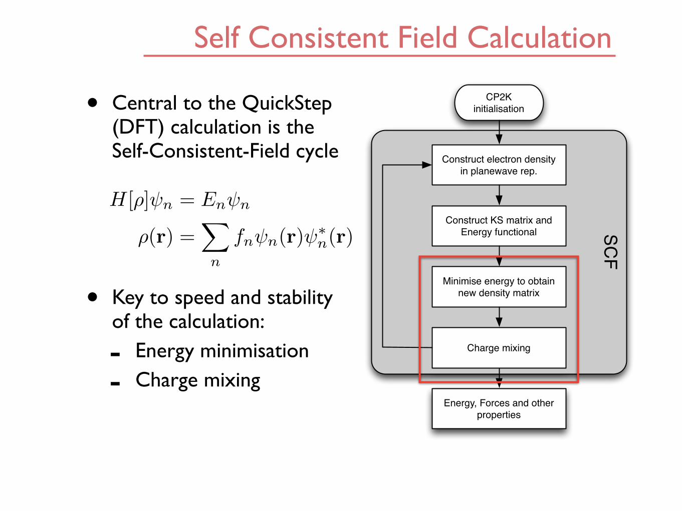
• Central to the QuickStep (DFT) calculation is the Self-Consistent-Field cycle

• Key to speed and stability of the calculation:

- Energy minimisation

- Charge mixing

Construct electron density in planewave rep.

CP2K initialisation

Construct KS matrix and Energy functional

Minimise energy to obtain new density matrix

Charge mixing

Energy, Forces and other properties

SCF

H[⇢] n = En n

⇢(r) =X

n

fn n(r) ⇤n(r)

Topics In This Talk

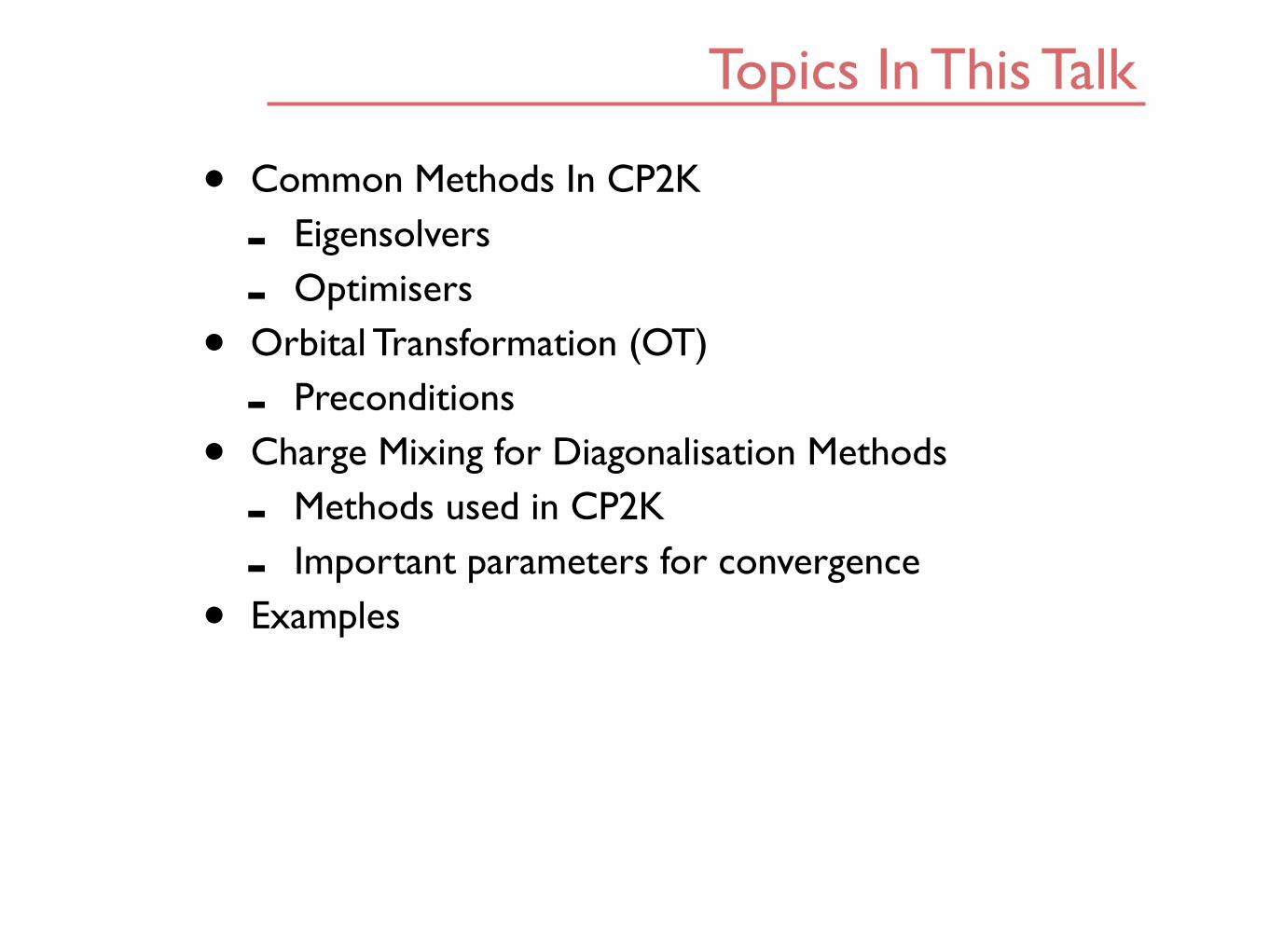
• Common Methods In CP2K

- Eigensolvers

- Optimisers

• Orbital Transformation (OT)

- Preconditions

• Charge Mixing for Diagonalisation Methods

- Methods used in CP2K

- Important parameters for convergence

• Examples

Eigensolvers In CP2K

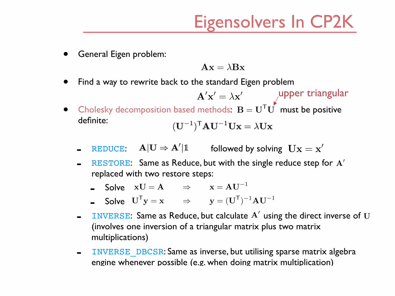
• General Eigen problem:

• Find a way to rewrite back to the standard Eigen problem

• Cholesky decomposition based methods: must be positive definite:

- REDUCE: followed by solving

- RESTORE: Same as Reduce, but with the single reduce step for replaced with two restore steps:

- Solve

- Solve

- INVERSE: Same as Reduce, but calculate using the direct inverse of (involves one inversion of a triangular matrix plus two matrix multiplications)

- INVERSE_DBCSR: Same as inverse, but utilising sparse matrix algebra engine whenever possible (e.g. when doing matrix multiplication)

A

0x

0 = �x0

Ax = �Bx

xU = A ) x = AU

�1

U

Ty = x ) y = (UT)�1

AU

�1

B = UTU

Ux = x

0

A0

A0

U

upper triangular

Eigensolvers In CP2K

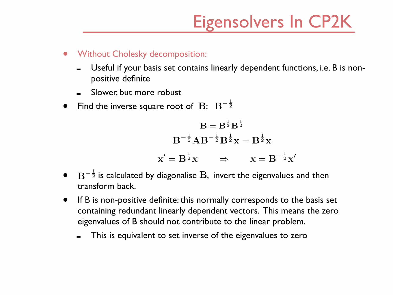
• Without Cholesky decomposition:

- Useful if your basis set contains linearly dependent functions, i.e. B is non-positive definite

- Slower, but more robust

• Find the inverse square root of :

• is calculated by diagonalise , invert the eigenvalues and then transform back.

• If B is non-positive definite: this normally corresponds to the basis set containing redundant linearly dependent vectors. This means the zero eigenvalues of B should not contribute to the linear problem.

- This is equivalent to set inverse of the eigenvalues to zero

B = B12B

12

B

� 12AB

� 12B

12x = B

12x

x

0 = B

12x ) x = B

� 12x

0

B B� 12

B� 12 B

Optimisers In CP2K

• Concerns with finding the local minimum of a function of many variables

• Steepest Decent:

- How much we travel along the gradient is determined by a line search to find the minimum of the function along the path

f(xn) = f(xn�1) + ↵rf(xn�1)

Optimisers In CP2K

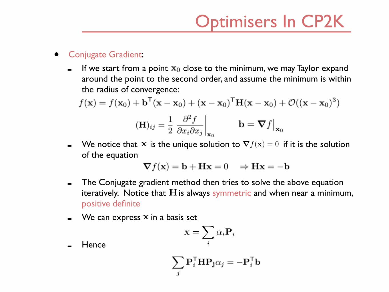
• Conjugate Gradient:

- If we start from a point close to the minimum, we may Taylor expand around the point to the second order, and assume the minimum is within the radius of convergence:

- We notice that is the unique solution to if it is the solution of the equation

- The Conjugate gradient method then tries to solve the above equation iteratively. Notice that is always symmetric and when near a minimum, positive definite

- We can express in a basis set

- Hence

x

x

x =X

i

↵iPi

H

rf(x) = 0

Optimisers In CP2K

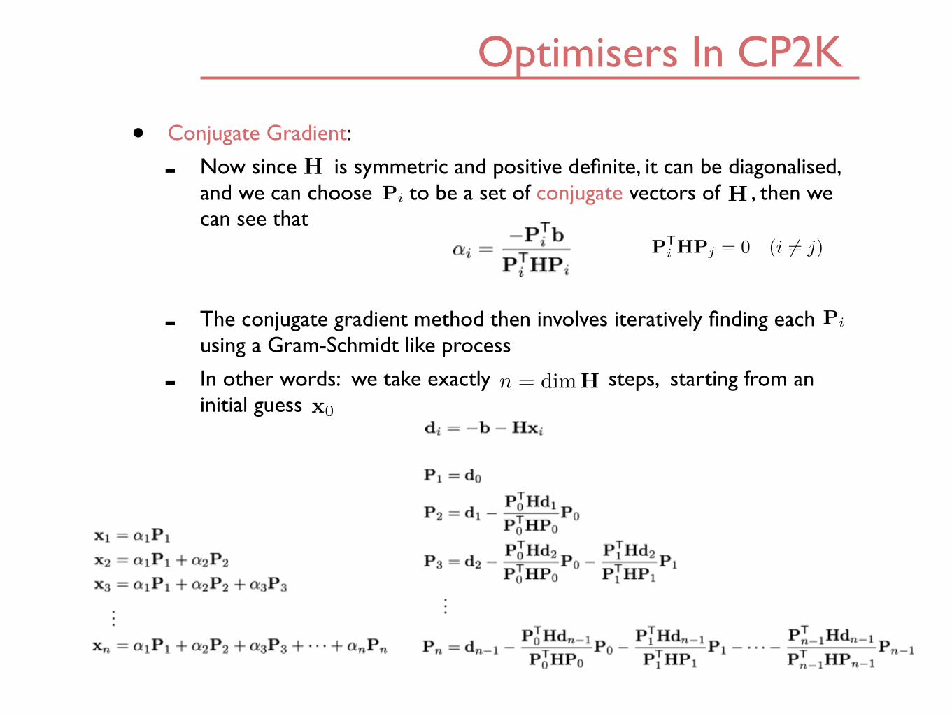
• Conjugate Gradient:

- Now since is symmetric and positive definite, it can be diagonalised, and we can choose to be a set of conjugate vectors of , then we can see that

- The conjugate gradient method then involves iteratively finding each using a Gram-Schmidt like process

- In other words: we take exactly steps, starting from an initial guess

HPi H

Pi

n = dimH

PTi HPj = 0 (i 6= j)

x0

Optimisers In CP2K

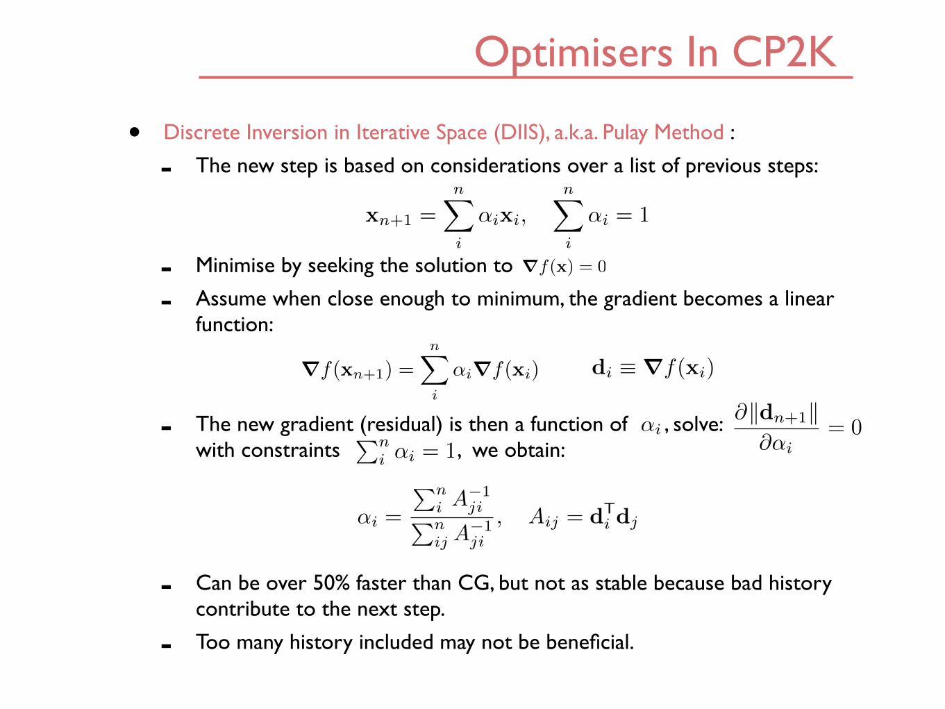
• Discrete Inversion in Iterative Space (DIIS), a.k.a. Pulay Method :

- The new step is based on considerations over a list of previous steps:

- Minimise by seeking the solution to

- Assume when close enough to minimum, the gradient becomes a linear function:

- The new gradient (residual) is then a function of , solve: with constraints , we obtain:

- Can be over 50% faster than CG, but not as stable because bad history contribute to the next step.

- Too many history included may not be beneficial.

xn+1 =nX

i

↵ixi,nX

i

↵i = 1

rf(x) = 0

rf(xn+1) =nX

i

↵irf(xi) di ⌘ rf(xi)

↵iPni ↵i = 1

@kdn+1k@↵i

= 0

↵i =

Pni A

�1jiPn

ij A�1ji

, Aij = dTi dj

Optimisers In CP2K

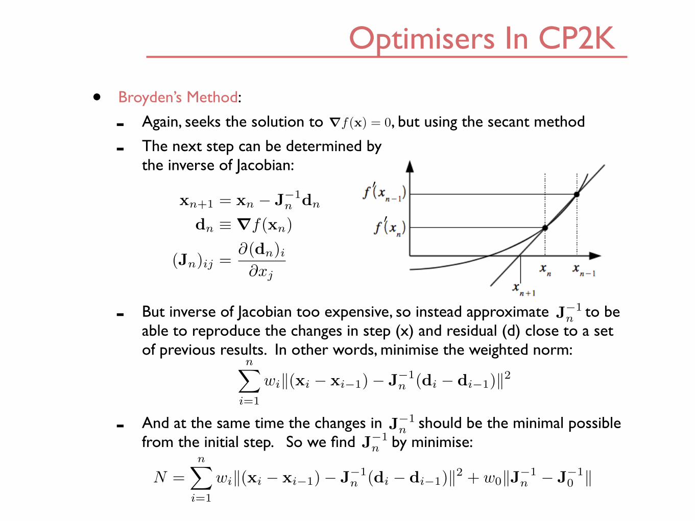
• Broyden’s Method:

- Again, seeks the solution to , but using the secant method

- The next step can be determined by the inverse of Jacobian:

- But inverse of Jacobian too expensive, so instead approximate to be able to reproduce the changes in step (x) and residual (d) close to a set of previous results. In other words, minimise the weighted norm:

- And at the same time the changes in should be the minimal possible from the initial step. So we find by minimise:

rf(x) = 0

0

0xn+1 = xn � J

�1n dn

dn ⌘ rf(xn)

(Jn)ij =@(dn)i@xj

N =nX

i=1

wik(xi � xi�1)� J

�1n (di � di�1)k2 + w0kJ�1

n � J

�10 k

J�1n

nX

i=1

wik(xi � xi�1)� J

�1n (di � di�1)k2

J�1n

J�1n

Orbital Transform

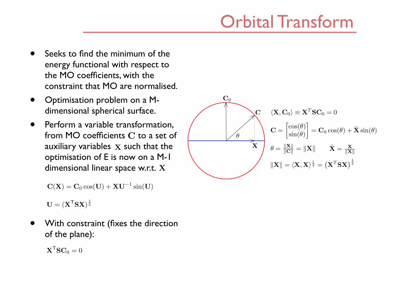
• Seeks to find the minimum of the energy functional with respect to the MO coefficients, with the constraint that MO are normalised.

• Optimisation problem on a M-dimensional spherical surface.

• Perform a variable transformation, from MO coefficients to a set of auxiliary variables such that the optimisation of E is now on a M-1 dimensional linear space w.r.t.

• With constraint (fixes the direction of the plane):

Direction of steepest decent

on E surface tangent to

manifold at ngeodesic

correction

Constraint manifold for CTSC = 1

Cn

Cn+1

Direction of steepest decent

on E surface tangent to

manifold at n

Constraint manifold for XTSC0 = 0

Xn+1

Xn

CX

X

U = (XTSX)12

C(X) = C0 cos(U) +XU�1sin(U)

XTSC0 = 0

Orbital Transform

• Seeks to find the minimum of the energy functional with respect to the MO coefficients, with the constraint that MO are normalised.

• Optimisation problem on a M-dimensional spherical surface.

• Perform a variable transformation, from MO coefficients to a set of auxiliary variables such that the optimisation of E is now on a M-1 dimensional linear space w.r.t.

• With constraint (fixes the direction of the plane):

CX

X

U = (XTSX)12

C(X) = C0 cos(U) +XU�1sin(U)

XTSC0 = 0

C

C0

X

✓C =

cos(✓)sin(✓)

�= C0 cos(✓) + ˆX sin(✓)

ˆX =

XkXk

hX,C0i ⌘ XTSC0 = 0

kXk = hX,Xi 12=

�XTSX

� 12

✓ =

kXkkCk = kXk

Orbital Transform

• Computation of SIN and COS terms

- Can be calculated by diagonalisation: transforming to eigenspace, operate on eigenvalues, and then transform back. BUT too expensive.

- Use Taylor expansion: 2 or 3 order expansion already give machine precision.

- Calculate as part of the Taylor expansionU�1

cos(U) =

KX

i=0

(�1)

(2i)!(XTSX)

i

U�1 sin(U) =KX

i=0

(�1)i

(2i+ 1)!(XTSX)i

Orbital Transform

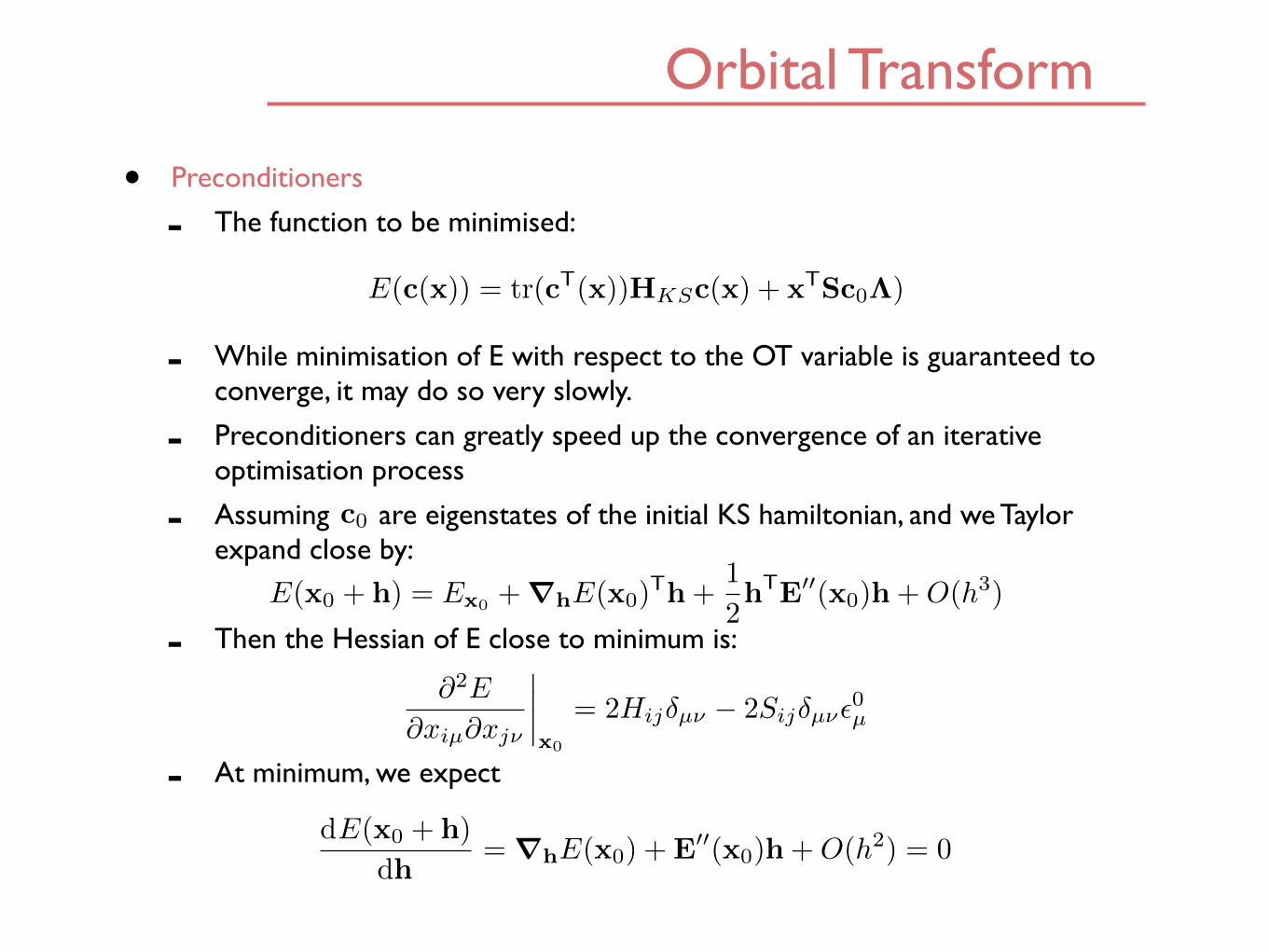
• Preconditioners

- The function to be minimised:

- While minimisation of E with respect to the OT variable is guaranteed to converge, it may do so very slowly.

- Preconditioners can greatly speed up the convergence of an iterative optimisation process

- Assuming are eigenstates of the initial KS hamiltonian, and we Taylor expand close by:

- Then the Hessian of E close to minimum is:

- At minimum, we expect

E(c(x)) = tr(cT(x))HKSc(x) + xTSc0⇤)

E(x0 + h) = Ex0 +r

h

E(x0)Th+

1

2h

TE

00(x0)h+O(h3)

dE(x0 + h)

dh= rhE(x0) +E

00(x0)h+O(h2) = 0

@2E

@xiµ@xj⌫

��x0

= 2Hij�µ⌫ � 2Sij�µ⌫✏0µ

c0

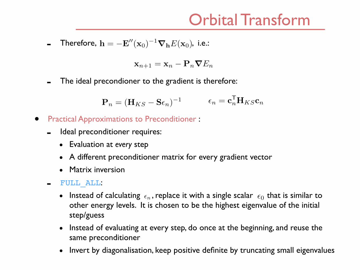
Orbital Transform- Therefore, , i.e.:

- The ideal precondioner to the gradient is therefore:

• Practical Approximations to Preconditioner :

- Ideal preconditioner requires:

• Evaluation at every step

• A different preconditioner matrix for every gradient vector

• Matrix inversion

- FULL_ALL:

• Instead of calculating , replace it with a single scalar that is similar to other energy levels. It is chosen to be the highest eigenvalue of the initial step/guess

• Instead of evaluating at every step, do once at the beginning, and reuse the same preconditioner

• Invert by diagonalisation, keep positive definite by truncating small eigenvalues

h = �E

00(x0)�1rhE(x0)

Pn = (HKS � S✏n)�1

xn+1 = xn �PnrEn

✏n = cTnHKScn

✏n ✏0

Orbital Transform- FULL_KINETIC

• Same as FULL_ALL, except only use kinetic energy part of KS matrix.

• This gives sparse matrices, and can be taken advantage of using DBCSR based methods

- FULL_SINGLE

• Same as FULL_ALL, however, only use the block diagonal parts of

• In other words, only on-site terms are considered by the preconditioner

• Much faster, as each block can be calculated separately

- FULL_SINGLE_INVERSE

• Same as FULL_SINGLE, but with the inversion process replaced by Cholesky process. Only works if is already positive definite.

• Therefore less robust, but more efficient than FULL_SINGLE

- FULL_S_INVERSE

• Ignore the KS matrix contribution all together, and utilise Cholesky decomposition of the full overlap matrix

• Generally avoid

- NONE

• Not recommended…

HKS � S✏0

HKS � S✏0

Orbital Transform• Inner and Outer SCF/OT minimisation Loop :

- Relevant only for OT:

- KS matrix is updated at every OT minimisation step: minimisation and SCF happening at the same time

- Inner Loop: Preconditioner is calculated at the begging of the loop, and remains constant throughout the inner loop

- Outer Loop: Loops over the inner loop, this means the preconditioner is updated at every outer loop step

- Tips for OT convergence:

• If inner loop is converging slowly, try to reduce the number of allowed iterations in the inner loop, and increase the number of iterations allowed for the outer loop.

• This effectively forces the preconditioner to be updated more frequently

Mixing Methods for Diagonalisation• Diagonalisation:

- Solves the generalised eigen problem:

- Uses any one of the eigensolvers implemented in CP2K

- Density matrix can be constructed from the MOs.

- Occupy the MOs from the lowest energy up, until total number of electrons has reached.

• This gives Fermi energy

• Allows the opportunity to introduce smearing into the occupancy

- From the density matrix, we can obtain electron charge, and this is then mixed back into the KS Hamiltonian, to complete the SCF loop

HKSc = �Sc

Pij =X

n

fncincjn

Mixing Methods for Diagonalisation• Smearing:

- Integer occupation numbers: discontinuity at Fermi energy.

- If Fermi energy is close to a number of MOs, a small variation of MO energies can lead to a jump in total energy, due to the electrons either occupy or leave a particular orbital completely

• This brings havoc to SCF optimisers, because all numerical optimisers work on the basis that functions they try to minimise is continuous and (at least once or twice) differentiable.

- Not a problem if the Fermi energy is in a band gap. Is a problem for metals.

0 0.5 1 1.5 2

0

0.2

0.4

0.6

0.8

1- Smearing: replace the step function

of occupancy with a smooth function of the similar shape, with smoothness controlled by a parametric temperature

- The higher the smearing temperature, the less resolution (system size) required for the band structure, but also less accurate

Mixing Methods for Diagonalisation• Broyden / Pulay Mixing

- The same as Broyden / DIIS optimisation method

- Solving for

- Broyden mixing is very similar to Pulay mixing, but slightly faster and somewhat more robust, as it does not involve matrix inversion

• Kerker Preconditioning (automatically turns on Pulay):

- Solve SCF convergence issues caused by large changes in the Hartree energy due to the changes in charge density that are far apart at every iteration step.

- The large change in Hartree energy then causes a corresponding reaction correction in the next output density, leading to a phenomenon referred to as “charge sloshing”.

- The problem can be solved by performing charge mixing in reciprocal space, and change the mixing parameter A to a preconditioner:

R[⇢in] = ⇢out � ⇢in = 0

A ! Aq2

q2 +B2Long range change correspond to

small q, and its contribution goes to 0

Examples

&SCF SCF_GUESS ATOMIC EPS_SCF 1.0E-06 MAX_SCF 200 &OT ON MINIMIZER DIIS PRECONDITIONER FULL_SINGLE_INVERSE &END OT &OUTER_SCF MAX_SCF 10 &END OUTER_SCF &PRINT &RESTART OFF &END RESTART &END PRINT &END SCF

If you have a restart file, use RESTART

64 water box

Examples SCF WAVEFUNCTION OPTIMIZATION

----------------------------------- OT --------------------------------------- Minimizer : DIIS : direct inversion in the iterative subspace using 7 DIIS vectors safer DIIS on Preconditioner : FULL_SINGLE_INVERSE : inversion of H + eS - 2*(Sc)(c^T*H*c+const)(Sc)^T Precond_solver : DEFAULT stepsize : 0.08000000 energy_gap : 0.08000000 eps_taylor : 0.10000E-15 max_taylor : 4 ----------------------------------- OT ---------------------------------------

Step Update method Time Convergence Total energy Change ------------------------------------------------------------------------------

Trace(PS): 512.0000000000 Electronic density on regular grids: -512.0000014959 -0.0000014959 Core density on regular grids: 512.0000000045 0.0000000045 Total charge density on r-space grids: -0.0000014914 Total charge density g-space grids: -0.0000014914

1 OT DIIS 0.80E-01 1.9 0.02242151 -1059.3825079557 -1.06E+03


2 OT DIIS 0.80E-01 1.2 0.01583191 -1079.2016155971 -1.98E+01



149 OT DIIS 0.80E-01 1.2 0.00000102 -1101.0377081868 -3.67E-07


150 OT DIIS 0.80E-01 1.2 0.00000101 -1101.0377086068 -4.20E-07


151 OT DIIS 0.80E-01 1.2 0.00000101 -1101.0377089336 -3.27E-07


152 OT DIIS 0.80E-01 1.2 0.00000100 -1101.0377093306 -3.97E-07


153 OT DIIS 0.80E-01 1.2 0.00000100 -1101.0377096545 -3.24E-07

*** SCF run converged in 153 steps ***

Examples

&SCF SCF_GUESS ATOMIC EPS_SCF 1.0E-06 MAX_SCF 200 &OT ON MINIMIZER DIIS PRECONDITIONER FULL_ALL &END OT &OUTER_SCF MAX_SCF 10 &END OUTER_SCF &PRINT &RESTART OFF &END RESTART &END PRINT &END SCF

64 water box

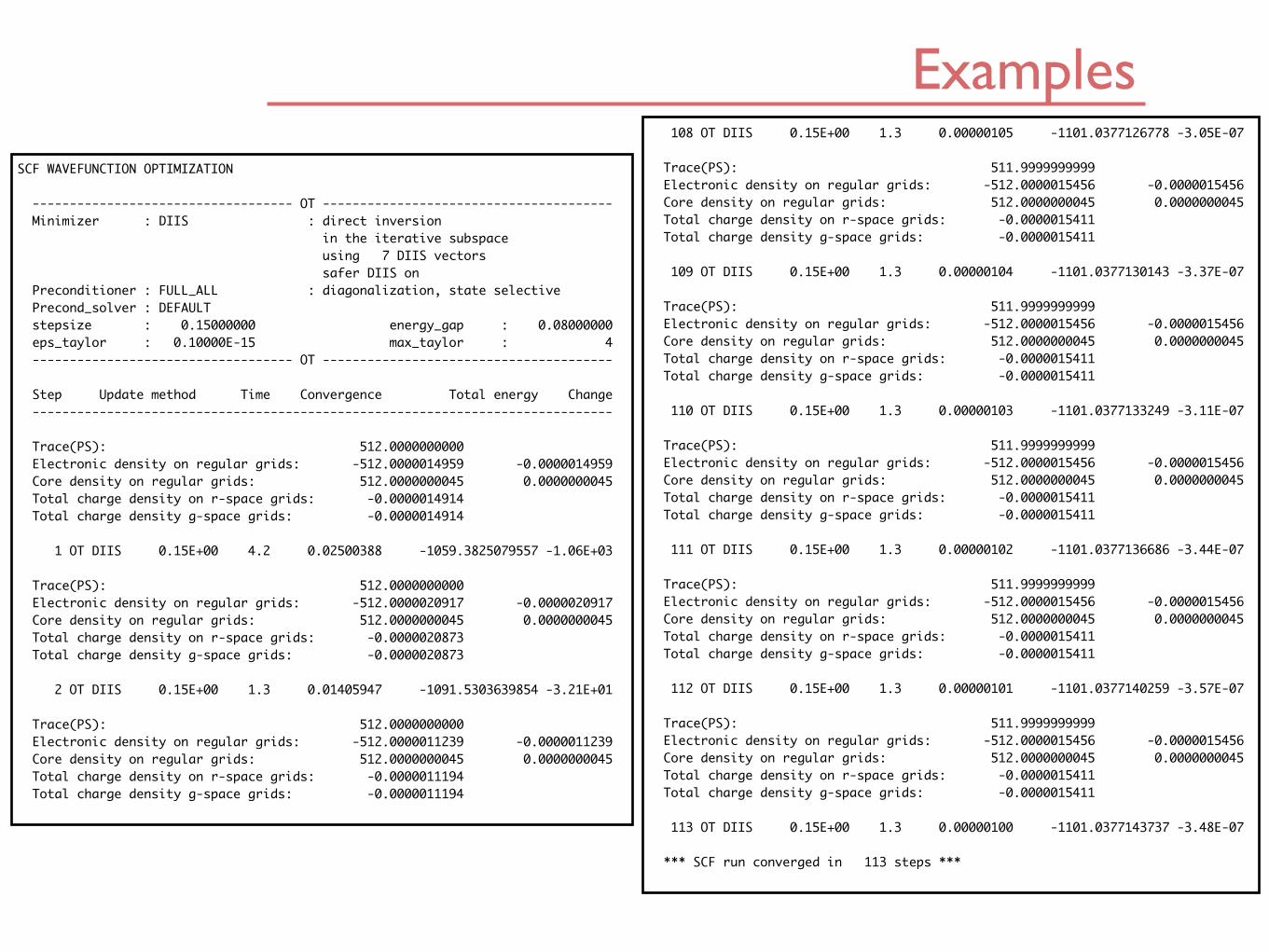
ExamplesSCF WAVEFUNCTION OPTIMIZATION

----------------------------------- OT --------------------------------------- Minimizer : DIIS : direct inversion in the iterative subspace using 7 DIIS vectors safer DIIS on Preconditioner : FULL_ALL : diagonalization, state selective Precond_solver : DEFAULT stepsize : 0.15000000 energy_gap : 0.08000000 eps_taylor : 0.10000E-15 max_taylor : 4 ----------------------------------- OT ---------------------------------------



1 OT DIIS 0.15E+00 4.2 0.02500388 -1059.3825079557 -1.06E+03


2 OT DIIS 0.15E+00 1.3 0.01405947 -1091.5303639854 -3.21E+01


108 OT DIIS 0.15E+00 1.3 0.00000105 -1101.0377126778 -3.05E-07


109 OT DIIS 0.15E+00 1.3 0.00000104 -1101.0377130143 -3.37E-07


110 OT DIIS 0.15E+00 1.3 0.00000103 -1101.0377133249 -3.11E-07


111 OT DIIS 0.15E+00 1.3 0.00000102 -1101.0377136686 -3.44E-07


112 OT DIIS 0.15E+00 1.3 0.00000101 -1101.0377140259 -3.57E-07


113 OT DIIS 0.15E+00 1.3 0.00000100 -1101.0377143737 -3.48E-07


Examples

&SCF SCF_GUESS ATOMIC EPS_SCF 1.0E-06 MAX_SCF 20 &OT ON MINIMIZER DIIS PRECONDITIONER FULL_ALL &END OT &OUTER_SCF MAX_SCF 100 &END OUTER_SCF &PRINT &RESTART OFF &END RESTART &END PRINT &END SCF

64 water box

Examples

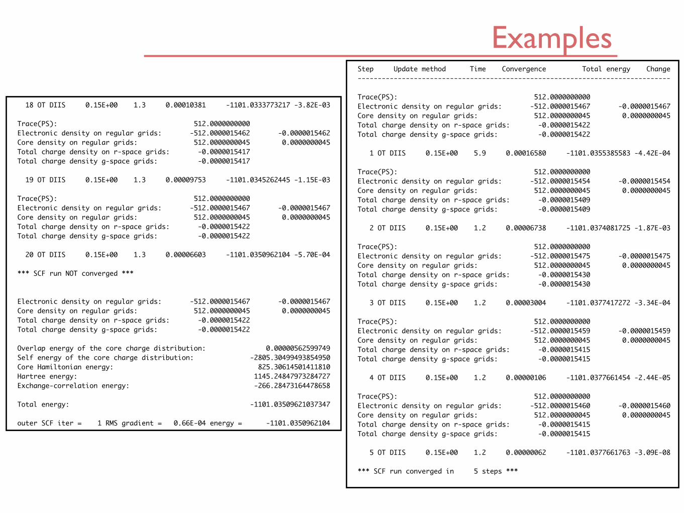
18 OT DIIS 0.15E+00 1.3 0.00010381 -1101.0333773217 -3.82E-03


19 OT DIIS 0.15E+00 1.3 0.00009753 -1101.0345262445 -1.15E-03


20 OT DIIS 0.15E+00 1.3 0.00006603 -1101.0350962104 -5.70E-04

*** SCF run NOT converged ***

Electronic density on regular grids: -512.0000015467 -0.0000015467 Core density on regular grids: 512.0000000045 0.0000000045 Total charge density on r-space grids: -0.0000015422 Total charge density g-space grids: -0.0000015422

Overlap energy of the core charge distribution: 0.00000562599749 Self energy of the core charge distribution: -2805.30499493854950 Core Hamiltonian energy: 825.30614501411810 Hartree energy: 1145.24847973284727 Exchange-correlation energy: -266.28473164478658

Total energy: -1101.03509621037347

outer SCF iter = 1 RMS gradient = 0.66E-04 energy = -1101.0350962104



1 OT DIIS 0.15E+00 5.9 0.00016580 -1101.0355385583 -4.42E-04


2 OT DIIS 0.15E+00 1.2 0.00006738 -1101.0374081725 -1.87E-03


3 OT DIIS 0.15E+00 1.2 0.00003004 -1101.0377417272 -3.34E-04


4 OT DIIS 0.15E+00 1.2 0.00000106 -1101.0377661454 -2.44E-05


5 OT DIIS 0.15E+00 1.2 0.00000062 -1101.0377661763 -3.09E-08


Examples &SCF SCF_GUESS ATOMIC EPS_SCF 1.0E-6 MAX_SCF 500 ADDED_MOS 200 CHOLESKY INVERSE &SMEAR ON METHOD FERMI_DIRAC ELECTRONIC_TEMPERATURE [K] 300 &END SMEAR &DIAGONALIZATION ALGORITHM STANDARD &END DIAGONALIZATION &MIXING METHOD DIRECT_P_MIXING ALPHA 0.5 &END MIXING &OUTER_SCF EPS_SCF 1.0E-6 MAX_SCF 1 &END OUTER_SCF &END SCF

Au128 bulk

Examples

Step Update method Time Convergence Total energy Change ------------------------------------------------------------------------------ 1 P_Mix/Diag. 0.50E+00 2.1 0.41056021 -2133.4408435676 -2.13E+03 2 P_Mix/Diag. 0.50E+00 3.2 0.20432922 -2132.0776002852 1.36E+00 3 P_Mix/Diag. 0.50E+00 3.2 0.10741372 -2131.3677551799 7.10E-01 4 P_Mix/Diag. 0.50E+00 3.2 0.05420394 -2131.0080867703 3.60E-01 5 DIIS/Diag. 0.39E-03 3.2 0.02722180 -2130.8276990683 1.80E-01 6 DIIS/Diag. 0.19E-03 3.1 0.00062404 -2130.6473761946 1.80E-01 7 DIIS/Diag. 0.84E-04 3.2 0.00050993 -2130.6473778175 -1.62E-06 8 DIIS/Diag. 0.63E-04 3.2 0.00021250 -2130.6473781683 -3.51E-07 9 DIIS/Diag. 0.11E-03 3.2 0.00019003 -2130.6473780859 8.24E-08 10 DIIS/Diag. 0.29E-03 3.1 0.00037131 -2130.6473764995 1.59E-06 11 DIIS/Diag. 0.34E-03 3.2 0.00045761 -2130.6473757354 7.64E-07 12 DIIS/Diag. 0.10E-02 3.2 0.00121294 -2130.6473574307 1.83E-05 13 DIIS/Diag. 0.47E-03 3.1 0.00355236 -2130.6473668667 -9.44E-06 14 DIIS/Diag. 0.74E-02 3.1 0.00485367 -2130.6464389964 9.28E-04 15 DIIS/Diag. 0.80E-02 3.1 0.01204111 -2130.6462412097 1.98E-04 16 DIIS/Diag. 0.10E-01 3.1 0.00709698 -2130.6441536117 2.09E-03 17 DIIS/Diag. 0.73E-02 3.1 0.06036011 -2130.6454804871 -1.33E-03 18 DIIS/Diag. 0.32E-01 3.1 0.07606048 -2130.6085108701 3.70E-02 19 P_Mix/Diag. 0.50E+00 3.1 1.20934863 -2130.4320575334 1.76E-01 20 P_Mix/Diag. 0.50E+00 3.1 164.38141403 -2083.0458429170 4.74E+01 21 P_Mix/Diag. 0.50E+00 3.1 484.77129296 642.3682176809 2.73E+03 22 P_Mix/Diag. 0.50E+00 3.1 242.49533726 680.0967740982 3.77E+01 23 P_Mix/Diag. 0.50E+00 3.1 108.28073503 713.7098573905 3.36E+01 24 P_Mix/Diag. 0.50E+00 3.1 133.38323194 -83.2160327233 -7.97E+02 25 P_Mix/Diag. 0.50E+00 3.1 243.65162842 257.9355830764 3.41E+02 26 P_Mix/Diag. 0.50E+00 3.1 360.75338107 804.4210109712 5.46E+02 27 P_Mix/Diag. 0.50E+00 3.2 423.28363111 790.1670568787 -1.43E+01 28 P_Mix/Diag. 0.50E+00 3.1 527.98757101 1358.0740107382 5.68E+02 29 P_Mix/Diag. 0.50E+00 3.1 467.44558067 1279.1848521006 -7.89E+01 30 P_Mix/Diag. 0.50E+00 3.1 511.11190255 1700.0469627750 4.21E+02 31 P_Mix/Diag. 0.50E+00 3.1 531.81962633 1488.0293045448 -2.12E+02 32 P_Mix/Diag. 0.50E+00 3.1 469.22980247 1449.5252473273 -3.85E+01

274 P_Mix/Diag. 0.50E+00 3.1 496.18271982 1433.1258409018 -2.52E+02 275 P_Mix/Diag. 0.50E+00 3.1 465.21950527 1708.0865674753 2.75E+02 276 P_Mix/Diag. 0.50E+00 3.2 526.35992000 1701.9896437225 -6.10E+00 277 P_Mix/Diag. 0.50E+00 3.1 500.55201331 1429.0695309273 -2.73E+02 278 P_Mix/Diag. 0.50E+00 3.1 452.47323777 1685.6997235986 2.57E+02 279 P_Mix/Diag. 0.50E+00 3.1 525.66284299 1726.0727258188 4.04E+01 280 P_Mix/Diag. 0.50E+00 3.1 504.85174061 1437.1005594299 -2.89E+02 281 P_Mix/Diag. 0.50E+00 3.1 452.73958110 1626.9128568615 1.90E+02 282 P_Mix/Diag. 0.50E+00 3.2 524.88774970 1767.5496813722 1.41E+02 283 P_Mix/Diag. 0.50E+00 3.1 509.84684807 1454.1863412940 -3.13E+02 284 P_Mix/Diag. 0.50E+00 3.1 424.76338293 1583.5008811158 1.29E+02 285 P_Mix/Diag. 0.50E+00 3.1 516.88135732 1784.1133181315 2.01E+02 286 P_Mix/Diag. 0.50E+00 3.1 514.48307366 1475.1702369153 -3.09E+02 287 P_Mix/Diag. 0.50E+00 3.1 429.02575267 1494.4059971253 1.92E+01 288 P_Mix/Diag. 0.50E+00 3.2 505.84474236 1762.0172683978 2.68E+02 289 P_Mix/Diag. 0.50E+00 3.1 521.09854796 1519.1104495575 -2.43E+02 290 P_Mix/Diag. 0.50E+00 3.2 460.28042402 1463.1850194878 -5.59E+01 291 P_Mix/Diag. 0.50E+00 3.1 494.65034012 1736.5367974686 2.73E+02 292 P_Mix/Diag. 0.50E+00 3.1 523.62795354 1561.0634325581 -1.75E+02 293 P_Mix/Diag. 0.50E+00 3.1 470.92963686 1458.4095785993 -1.03E+02 294 P_Mix/Diag. 0.50E+00 3.1 489.94822751 1740.7536880093 2.82E+02 295 P_Mix/Diag. 0.50E+00 3.1 527.88371821 1586.4713619002 -1.54E+02 296 P_Mix/Diag. 0.50E+00 3.1 477.46948475 1461.2599044466 -1.25E+02 297 P_Mix/Diag. 0.50E+00 3.1 481.52741519 1744.2498516733 2.83E+02 298 P_Mix/Diag. 0.50E+00 3.1 528.64978975 1631.2670959487 -1.13E+02 299 P_Mix/Diag. 0.50E+00 3.1 483.01432540 1447.7674793116 -1.83E+02 300 P_Mix/Diag. 0.50E+00 3.1 475.21476950 1734.9217161865 2.87E+02 301 P_Mix/Diag. 0.50E+00 3.1 527.70245328 1640.9047892819 -9.40E+01 302 P_Mix/Diag. 0.50E+00 3.1 485.65879289 1448.0327123002 -1.93E+02 303 P_Mix/Diag. 0.50E+00 3.1 474.33206574 1735.1993514743 2.87E+02 304 P_Mix/Diag. 0.50E+00 3.1 528.41442815 1652.4630012861 -8.27E+01 305 P_Mix/Diag. 0.50E+00 3.1 487.89310966 1441.5618979731 -2.11E+02 306 P_Mix/Diag. 0.50E+00 3.1 472.80773473 1735.6753322017 2.94E+02 307 P_Mix/Diag. 0.50E+00 3.1 528.03454596 1664.1188498883 -7.16E+01 308 P_Mix/Diag. 0.50E+00 3.1 489.55606395 1439.4935858980 -2.25E+02 309 P_Mix/Diag. 0.50E+00 3.2 471.87729366 1733.8307029231 2.94E+02 310 P_Mix/Diag. 0.50E+00 3.1 527.88042982 1669.9038337698 -6.39E+01

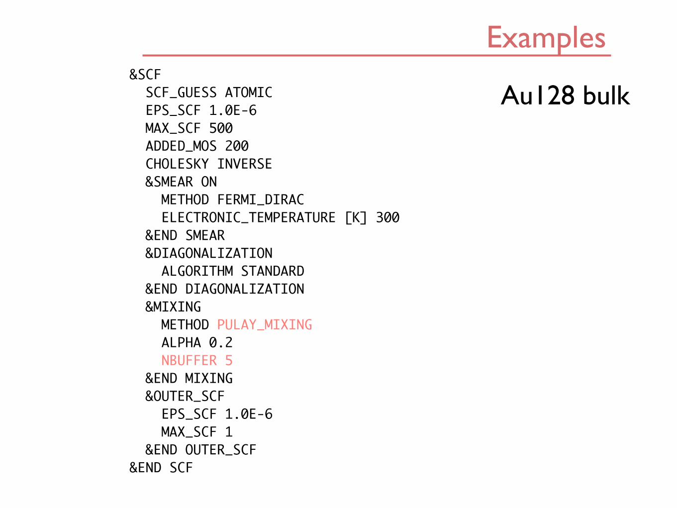
Examples &SCF SCF_GUESS ATOMIC EPS_SCF 1.0E-6 MAX_SCF 500 ADDED_MOS 200 CHOLESKY INVERSE &SMEAR ON METHOD FERMI_DIRAC ELECTRONIC_TEMPERATURE [K] 300 &END SMEAR &DIAGONALIZATION ALGORITHM STANDARD &END DIAGONALIZATION &MIXING METHOD PULAY_MIXING ALPHA 0.2 NBUFFER 5 &END MIXING &OUTER_SCF EPS_SCF 1.0E-6 MAX_SCF 1 &END OUTER_SCF &END SCF

Au128 bulk

Examples

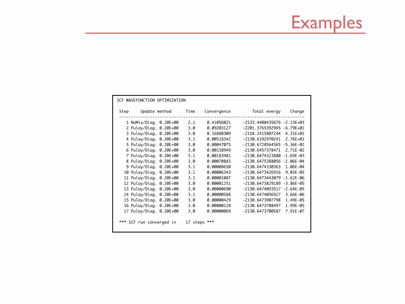
SCF WAVEFUNCTION OPTIMIZATION

Step Update method Time Convergence Total energy Change ------------------------------------------------------------------------------ 1 NoMix/Diag. 0.20E+00 2.1 0.41056021 -2133.4408435676 -2.13E+03 2 Pulay/Diag. 0.20E+00 3.0 0.09203127 -2201.3765392945 -6.79E+01 3 Pulay/Diag. 0.20E+00 3.0 0.16880309 -2158.2415807244 4.31E+01 4 Pulay/Diag. 0.20E+00 3.1 0.00518342 -2130.6192970241 2.76E+01 5 Pulay/Diag. 0.20E+00 3.0 0.00047075 -2130.6728564565 -5.36E-02 6 Pulay/Diag. 0.20E+00 3.0 0.00158949 -2130.6457378471 2.71E-02 7 Pulay/Diag. 0.20E+00 3.1 0.00183981 -2130.6474323880 -1.69E-03 8 Pulay/Diag. 0.20E+00 3.0 0.00070883 -2130.6475388056 -1.06E-04 9 Pulay/Diag. 0.20E+00 3.1 0.00008650 -2130.6474330363 1.06E-04 10 Pulay/Diag. 0.20E+00 3.1 0.00006343 -2130.6473426916 9.03E-05 11 Pulay/Diag. 0.20E+00 3.1 0.00001087 -2130.6473443079 -1.62E-06 12 Pulay/Diag. 0.20E+00 3.0 0.00001251 -2130.6473829189 -3.86E-05 13 Pulay/Diag. 0.20E+00 3.0 0.00000690 -2130.6474093517 -2.64E-05 14 Pulay/Diag. 0.20E+00 3.1 0.00000588 -2130.6474056927 3.66E-06 15 Pulay/Diag. 0.20E+00 3.0 0.00000429 -2130.6473907798 1.49E-05 16 Pulay/Diag. 0.20E+00 3.0 0.00000128 -2130.6473708497 1.99E-05 17 Pulay/Diag. 0.20E+00 3.0 0.00000069 -2130.6473700587 7.91E-07


Examples &SCF SCF_GUESS ATOMIC EPS_SCF 1.0E-6 MAX_SCF 500 ADDED_MOS 200 CHOLESKY INVERSE &SMEAR ON METHOD FERMI_DIRAC ELECTRONIC_TEMPERATURE [K] 300 &END SMEAR &DIAGONALIZATION ALGORITHM STANDARD &END DIAGONALIZATION &MIXING METHOD BRYODEN_MIXING ALPHA 0.2 NBUFFER 5 &END MIXING &OUTER_SCF EPS_SCF 1.0E-6 MAX_SCF 1 &END OUTER_SCF &END SCF

Au128 bulk

Examples

SCF WAVEFUNCTION OPTIMIZATION

Step Update method Time Convergence Total energy Change ------------------------------------------------------------------------------ 1 NoMix/Diag. 0.20E+00 2.1 0.41056021 -2133.4408435676 -2.13E+03 2 Broy./Diag. 0.20E+00 3.0 0.09203127 -2201.3765392945 -6.79E+01 3 Broy./Diag. 0.20E+00 3.0 0.16796900 -2158.0252203875 4.34E+01 4 Broy./Diag. 0.20E+00 3.0 0.00119322 -2130.7623431374 2.73E+01 5 Broy./Diag. 0.20E+00 3.0 0.00354041 -2130.8401320934 -7.78E-02 6 Broy./Diag. 0.20E+00 3.0 0.00027721 -2130.6310148769 2.09E-01 7 Broy./Diag. 0.20E+00 3.0 0.00021364 -2130.6341596109 -3.14E-03 8 Broy./Diag. 0.20E+00 3.0 0.00096927 -2130.6425441433 -8.38E-03 9 Broy./Diag. 0.20E+00 3.0 0.00061032 -2130.6368211911 5.72E-03 10 Broy./Diag. 0.20E+00 3.0 0.00008199 -2130.6405099448 -3.69E-03 11 Broy./Diag. 0.20E+00 3.1 0.00004376 -2130.6475333293 -7.02E-03 12 Broy./Diag. 0.20E+00 3.1 0.00001638 -2130.6493205024 -1.79E-03 13 Broy./Diag. 0.20E+00 3.1 0.00001451 -2130.6486762850 6.44E-04 14 Broy./Diag. 0.20E+00 3.2 0.00001432 -2130.6482674682 4.09E-04 15 Broy./Diag. 0.20E+00 3.1 0.00001122 -2130.6476512837 6.16E-04 16 Broy./Diag. 0.20E+00 3.1 0.00000112 -2130.6472295415 4.22E-04 17 Broy./Diag. 0.20E+00 3.1 0.00000103 -2130.6472635676 -3.40E-05 18 Broy./Diag. 0.20E+00 3.1 0.00000112 -2130.6472999859 -3.64E-05 19 Broy./Diag. 0.20E+00 3.0 0.00000168 -2130.6473550000 -5.50E-05 20 Broy./Diag. 0.20E+00 3.0 0.00000144 -2130.6473964425 -4.14E-05 21 Broy./Diag. 0.20E+00 3.1 0.00000009 -2130.6474004989 -4.06E-06


scf methods2016_summer_school:... · 2016-08-24 · scf methods — diagonalisation &orbital...

Documents