scat wind retrieval simulator & fom
TRANSCRIPT

CFOSAT, Oct 2009
SCAT wind SCAT wind retrievalretrievalsimulatorsimulator & & FoMFoM
Royal Netherlands Meteorological [email protected]
Maria Belmonte Rivas, Jos de Kloe

CFOSAT, Oct 2009
Outline• Objective• SCAT Baseline and backup concepts• End-to-End Performance Study
– Input winds– Observation geometry– Instrumental and geophysical noise– Wind retrieval simulator– Figure of Merit
• Test cases• Conclusions

CFOSAT, Oct 2009
Objective• KNMI is responsible for
the End-to-End SCAT Performance Study for Post-EPS (2019):– To assess the wind retrieval performance– To support parameter optimization

CFOSAT, Oct 2009
Post EPS scatterometer (SCA) [baseline requirements and options]
• Spatial resolution (25 km)• Dynamic range (4-25 m/s)• Radiometric resolution (~3-10% at 4 m/s)• Swath coverage (95% in 48 hours for incidences between 20 and 60°)
I - Fixed beam (ASCAT type) II - Rotating beam (RFSCAT type)
Discarded: Ku-band, pencil beam, extended nadir coverage for ASCAT type
MetOp orbit Sun Sync with 820 km altitude

CFOSAT, Oct 2009
End-to-End Performance Study
1) Input wind vector
GMF
2) Observation geometry
Backscatter vector
+ Instrumental noise+ Geophysical noise
4) Wind retrieval
5) Figure of Merit (function of input wind, location on swath and system noise)
3)

CFOSAT, Oct 2009
SCA wind retrieval simulator (F90)
Input wind vector
GMFPseudo L1B file
Backscatter vector observation
Geophysical noise
Wind inversion
Observational likelihood
Output wind vector(first rank solution)
Pobs(Vout|Vin)( )
20 0,
22 01,...,
( , )1( , ) i GMF i
i N p i
wMLE w
MLE K
σ σ φφ
σ=
−=
QuikSCAT Kp =20%9 m/s @ 90 deg
Outer swath
CFOSAT, Oct 2009
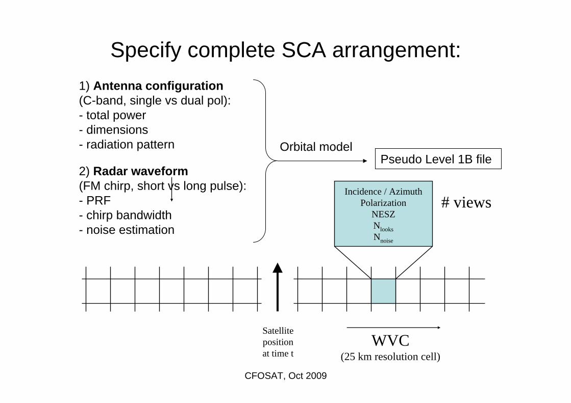
Specify complete SCA arrangement:1) Antenna configuration (C-band, single vs dual pol):- total power- dimensions - radiation pattern
2) Radar waveform(FM chirp, short vs long pulse):- PRF- chirp bandwidth- noise estimation
Pseudo Level 1B fileOrbital model
Incidence / AzimuthPolarization
NESZNlooksNnoise
WVC(25 km resolution cell)
Satellitepositionat time t
# views

CFOSAT, Oct 2009
2) Observation geometry
Pseudo L1B file(simulated swath coverage)
WVC(25 km resolution cell)
IncidenceAzimuth
PolSNRNlooksNnoise
Satellitepositionat time t
- Orbital model- Antenna/Pulse design- Spatial ground filter
# views

CFOSAT, Oct 2009
Radiometric resolution (NESZ and Kp)
lookslook
x yNA
Δ Δ=
noise s noiseN f T=
look range azimuthA = Δ Δ
( )
00
2
3 4
( )
4
B eq look
lookt TX RX
prop
k T T BNESZSNR APG G
R L
σλπ
+= =
⋅
1) NESZ (Noise Equivalent Sigma Zero) for a single look:
2) Number of looks per node:
3) Number of noise samples:
2 202
20
var{ } 1 1 1 11plooks noise
KN SNR N SNR
σσ
= = + +
Radiometric resolution:
(reduce speckle)
(noise estimation)

CFOSAT, Oct 2009
1) Input wind vector• Climatology distribution of wind inputs:
Weibull distribution in wind speeds (with maximum around 8 m/s) and uniform distribution in wind direction.

CFOSAT, Oct 2009
3) Instrumental & geophysical noise
( )0
2 220
var{ } 0.064( 16)gk vσσ
= = −r
( )20
22 20
var{ } 1 1 11plooks noise
kN SNR N SNR
σσ
= = + +
• Instrumental (radiometric) noise
• Geophysical noise
0 0 2 2(1 [0;1])GMF p gk k Nσ σ= + + ⋅Simulated observations

CFOSAT, Oct 2009
4) Wind retrieval – MLE and likelihood
20 0,
01,...,
( , )1( , )var{ }
i GMF i
i N i
wMLE w
MLEσ σ φ
φσ=
−=
( ) [ ]0 22; , ( , )obs NP u v MLE u vσ χ −=
• Multiple ambiguous solutions and broad maximaare limiting factors in wind retrieval performance.

CFOSAT, Oct 2009
4) Wind retrieval – worst cases
• Rotating beam (SeaWinds WVC=0)
• Fixed antennas (ASCAT WVC =0)

CFOSAT, Oct 2009
SCAT simulator verification tests
1) Verifying MLE statistics (“chi-square assumption”)
QSCAT (N = 4 views)
e-x/2
• Simulator MLE statisticsfollow 2 assumption at low noise levels.
• At higher noise levelsGMF loses its 2D surface quality and statisticsare modified accordingly!

CFOSAT, Oct 2009
SCAT simulator verification tests
2) Verifying observational likelihoods
(True wind input is 9 m/s @ 45 deg, 1000 simulator runs)
Expected SCAT Simulator

CFOSAT, Oct 2009
WVC =13
WVC =26
QSCAT
QSCAT
• SCAT Simulator is more realistic “than expected”.

CFOSAT, Oct 2009
4) Wind retrieval –background info
[ ]( ) ( )222ln(Probability) 2ln ( ) 2ln ;obs bg N bg bgJ J J MLE v N v vχ σ− = − = + = − − −
r r r
Best wind estimate
• Combined observation and NWP background cost functions:
[ ]22( , ) ( , )obs Np u v C MLE u vχ −= ( , ) ;bg bg bgp u v N v v σ = −
r r
Maximum likelihood
CFOSAT, Oct 2009
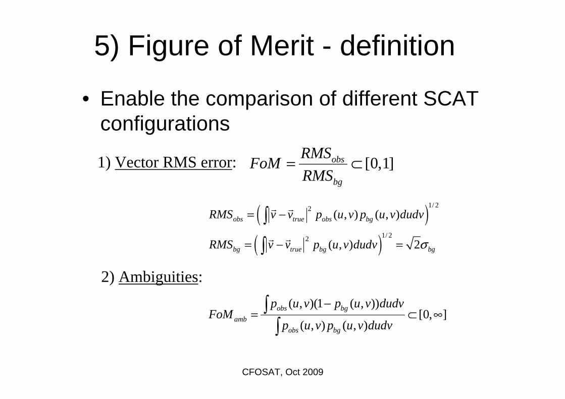
5) Figure of Merit - definition
• Enable the comparison of different SCAT configurations
[0,1]obs
bg
RMSFoMRMS
= ⊂
( )( )
1/ 22
1/ 22
( , ) ( , )
( , ) 2
obs true obs bg
bg true bg bg
RMS v v p u v p u v dudv
RMS v v p u v dudv σ
= −
= − =
r r
r r
( , )(1 ( , ))[0, ]
( , ) ( , )obs bg
ambobs bg
p u v p u v dudvFoM
p u v p u v dudv
−= ⊂ ∞
1) Vector RMS error:
2) Ambiguities:

CFOSAT, Oct 2009
Systematic biasesDetermined by skewness in observational likelihood:
• Example: True wind input with 9 m/s @ 30 deg features small wind speed bias but output wind direction seems drawn to 45 deg solution!
( , ) ( , )
( , ) ( , )
speed true obs true bg true
dir true obs true bg true
skew v v p v p v dv
skew p v p v d
φ φ
φ φ φ φ φ
= − ⋅
= − ⋅
skewness = mode - mean(in wind speed and direction)
u
v

CFOSAT, Oct 2009
Wind retrieval performancePobs(Vout|Vin) NWP background (5 m2/s2)
1) Wind Vector RMS error
2) Ambiguity susceptibility
3) Wind biases (skewness)Figu
re o
f Mer
it
( )1/ 22 2( ) ( )obs true obs bgRMS v v p v p v d v= −r r r r
For instance:
u
v

CFOSAT, Oct 2009
Wind retrieval performance9 m/s
5 m/s
9 m/s
13 m/sexamples

CFOSAT, Oct 2009
FoM – Test cases
better
worse
0.28 0.32 0.38 0.41
0.48 0.53 0.64 0.73
QSCATASCAT
1.19 1.57
1.14
1.591.20
2.852.872.10

CFOSAT, Oct 2009
FoM – Test cases
• For this wind input, ASCAT gives better background constrained information, although with more ambiguity.

CFOSAT, Oct 2009
Preliminary SCA assessment
ASCATtype
RFSCAT(1rpm)
RFSCAT(2rpm)
RFSCAT(3rpm)
Wind Vector RMS error across swath
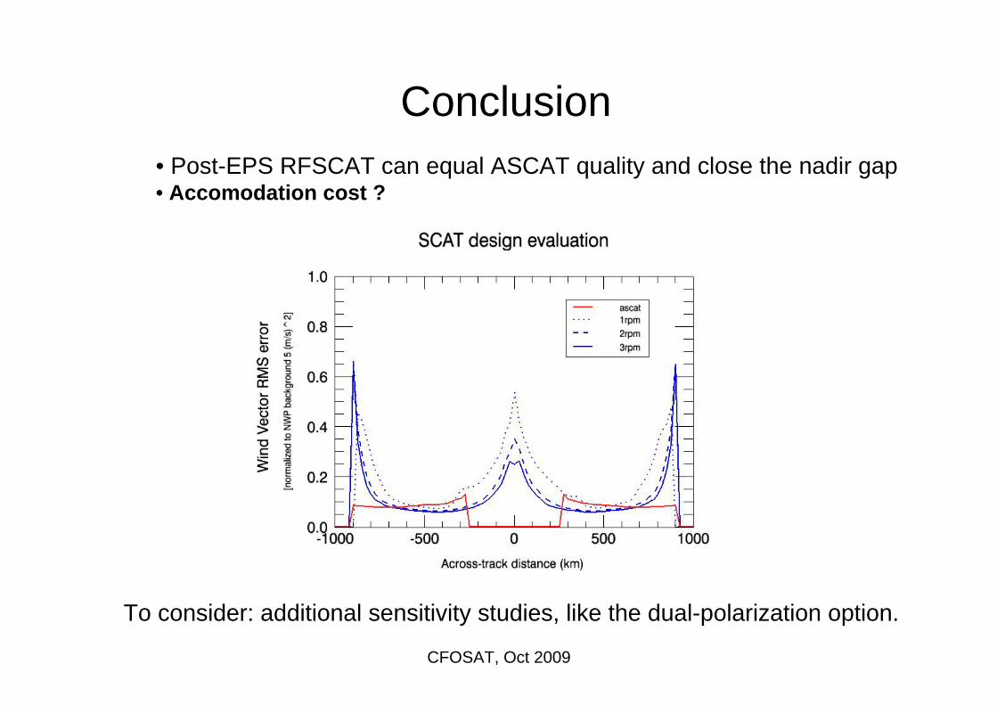
CFOSAT, Oct 2009
Conclusion• Post-EPS RFSCAT can equal ASCAT quality and close the nadir gap• Accomodation cost ?
To consider: additional sensitivity studies, like the dual-polarization option.