General rights Copyright and moral rights for the publications made accessible in the public portal are retained by the authors and/or other copyright owners and it is a condition of accessing publications that users recognise and abide by the legal requirements associated with these rights.

Users may download and print one copy of any publication from the public portal for the purpose of private study or research.

You may not further distribute the material or use it for any profit-making activity or commercial gain

You may freely distribute the URL identifying the publication in the public portal If you believe that this document breaches copyright please contact us providing details, and we will remove access to the work immediately and investigate your claim.

Downloaded from orbit.dtu.dk on: Feb 10, 2019

Scanning X-ray Imaging Techniques for Characterization of Energy Materials

Ayres Pereira da Cunha Ramos, Tiago João

Publication date:2019

Document VersionPublisher's PDF, also known as Version of record

Link back to DTU Orbit

Citation (APA):A. P. C. Ramos, T. J. (2019). Scanning X-ray Imaging Techniques for Characterization of Energy Materials.Technical University of Denmark (DTU).

Scanning X-ray Imaging Techniques

for Characterization of Energy Materials

Tiago J. A. P. C. Ramos

DTU Risø Campus 2018

i

Preface

This thesis was prepared in partial fulfilment of the requirements for the acqui-

sition of a PhD degree at the Technical University of Denmark (DTU). The work

here described was carried out in the period of September 2015 to September

2018 in the section of Imaging and Structural Analysis of the department of En-

ergy Conversion and Storage, under the supervision of Professor Jens Wenzel

Andreasen.

This work was funded by the Innovation Fund Denmark (Innovationsfonden)

within the CINEMA (alliance for ImagiNg and Modelling of Energy Applica-

tions). Part of the work was performed in collaboration with the NanoMAX

beamline from the MAX IV laboratory, as part of the EU project ESS MAX IV –

Cross Border Science and Society and subproject MAX4ESSFUN Cross Border

Network and Researcher Programme.

14th September 2018

Tiago Ramos

ii

iii

Summary

The large and ever-growing energy needs call for an urgent shift for sustainable energy

sources. Associated to the current production of energy is the emission of noxious gas-

es that among other undesirable effects contribute for an increase of the greenhouse

effect and consequently to global warming. From the currently available energy

sources, solar energy is the one with the biggest potential to fulfil our current and fu-

ture energetic needs. To date, the main factors impeding upscaling and mass produc-

tion of solar cell devices are associated to their high production costs or low efficien-

cies, for which fossil fuels are still economically competitive.

The performance of solar cells, especially those from second- and third-generation, is

largely determined by their micro- and nano-scale. To improve their conversion effi-

ciency, scientists must first be able to measure and characterize the nanostructure of

the devices produced by current synthesis methods, so that these may be improved or

tuned to fulfil a specific need.

Emerging X-ray imaging techniques, such as coherent diffractive imaging methods,

have the potential to reach extremely high resolutions and are well suited for this task.

Currently the available spatial resolution delivered by such methods is limited by the

X-ray beam properties and by the performance of the numerical algorithms used for

image reconstruction. Furthermore, the combination of different X-ray imaging meth-

ods allows for complementary information about the sample from which the local elec-

tronic and chemical compositions can be derived.

This thesis is devoted to the improvement of current X-ray scanning imaging methods.

Our main contributions lie in the development of numerical algorithms for image data

analysis of X-ray fluorescence and X-ray ptychography. More specifically the thesis

includes the theoretical background of the main types of X-ray-matter interaction, a

brief description of some X-ray scanning imaging techniques, the description of the

developed algorithms and the report of recent experimental measurements for the

characterization of third-generation kesterite solar cells.

iv

v

Resumé

Det store og evigt voksende energiforbrug kræver indtrængende et skift til bæredygti-

ge energikilder. Forbundet med den nuværende produktion af energi via fossile

brændsler er udledningen af skadelige gasser, der blandt andet bidrager til global op-

varmning gennem drivhuseffekten. Ud af de energikilder, vi har tilgængelige i dag, er

solenergi den med det største potentiale til at dække vores nuværende og fremtidige

energiforbrug. De største faktorer, der til dato har begrænset opskaleringen og masse-

produktionen af solceller, er forbundet med høje produktionsomkostninger eller lav

effektivitet, hvilket til stadighed gør fossile brændsler økonomisk konkurrencedygtige.

Effektiviteten af solceller, specielt den af anden- og tredjegenerationssolceller, er ho-

vedsageligt bestemt af deres morfologi på micro- og nanoskala. For at forbedre deres

effektivitet kræves en indsats fra videnskabsmænd imod at blive i stand til at måle og

karakterisere strukturen af de solceller, der bliver produceret og printet fra opløsning,

så disse metoder bliver forbedret eller tunet til at opfylde specifikke behov.

Nye røntgenbilledbehandlingsmetoder, såsom koherent diffraktionsbilledbehandling,

har potentialet til at nå ekstremt høje billedopløsninger og er godt egnet til denne op-

gave. Den nuværende rumlige opløsning, der er opnåelig med denne og lignende me-

toder, er begrænset af egenskaberne af røntgenstråler og af effektiviteten af de nume-

risk algoritmer, der bliver brugt til at rekonstruere billederne fra disse eksperimenter.

Desuden tillader kombinationen af forskellige røntgenbaserede målemetoder os at få

komplementær information om vores prøver, så deres lokale elektroniske og kemiske

komposition kan blive analyseret og bestemt.

Denne Ph.D.-afhandling er koncentreret omkring forbedringen af de nuværende bil-

ledbehandlingsmetoder for røntgenskanning. Vores største bidrag baserer sig på ud-

viklingen af numeriske algoritmer til billedanalyse af røntgenfluorescens og –

ptychografi. Mere specifikt inkluderer denne afhandling en teoretisk baggrund for et

udvalg af røntgenskanningsmetoder, samt beskrivelsen af de udviklede algoritmer og

nylige eksperimentelle målinger i forbindelse med karakteriseringen af tredjegenera-

tionssolceller baseret på kesteritter.

vi

vii

Acknowledgments

I would like to express my immense gratitude to all the people I had the opportunity to

meet and work with, without whom this work would have not been possible.

First, to my parents, for all their support, guidance, and positive influences in my life to

whom I dedicate this thesis. I must say that in the last three years I was blessed with an

extraordinary team of people that I will remember and keep for all years to come. If I

was to properly address each in specific, this section would most likely become a dom-

inant part of this thesis. Instead I would like to briefly thank my co-workers and

friends Aleksandr, Anders, Azat, Christian, Giovanni, Khadijeh, Lea, Marcial, Mariana,

Megha and Michael for their friendship, enriching discussions, generous smiles besides

all their help in scientific matters for which I am sure they know I am grateful.

Thank you Mike, Mégane, Pia, Jørgen and Aia for taking the “role” of my family, for

sharing a house, and life’s ups and downs in these last three years.

Thank you Jens, for your academic support, trust, patience, advices and kind words in

the moments of most need. Thank you Jakob and Martin for your wise teachings and

suggestions in the fields of tomography and numerical optimization that were crucial

for my understanding of these subjects.

I also take this opportunity to thank Dr. Alexander Björling, Dr. Gerardina Carbone for

their support during my external collaboration project, and to the anonymous referees

for their useful suggestions in our manuscripts.

Last but not least, to the love and light of my life Sofia and Heidi, for their endless love,

understanding and long waiting. I’m coming home now.

Ulteia et Suseia!

viii

ix

List of symbols and abbreviations

𝐀 – System Matrix

𝐁 – Magnetic field

𝐵0 – Amplitude of magnetic field

𝑐 – speed of light in vacuum

𝑑ps – Detector pixel size

𝐄 – Electric Field

𝐸0 – Amplitude of electric field

𝑒 – photon energy

e – Euler number

𝐹 – Fresnel number

ℱ – Two dimensional Fourier Transform

ℱ1 – One dimensional Fourier Transform

𝑓0 – Atomic form factor

𝑔𝐾𝛼 – Transition probability for 𝐾𝛼 emission

ℎ - Plank’s constant

𝐢 – imaginary unit √−1.

��, 𝒋, �� – spatial unit vectors

𝐼𝑝 – Absorption projection

𝐼0 – Flat field projection

𝐼𝐷 – Dark field projection

𝐼𝑁 – Flat field corrected absorption projection

𝐉 – Current density field

𝐽𝐾 – Absorption jump factor

𝐤 – wave vector

𝐾𝛼 – X-ray emission line

𝐿 – Distance from sample to detector

𝐿𝐿 – Longitudinal coherence length

𝐿𝑇 – Transverse coherence length

𝑁𝑒−/ℎ+coll – Number of collected electric charges

𝑁𝑒−/ℎ+gen

– Number of generated electric charges

𝑛 – Refractive index

𝑂 – Object function

𝑃𝑨, 𝑃𝑩 - Projector operators in the Difference Map algorithm

𝑃 – Probe or illumination function

𝒑 – photon momentum

x

𝑝𝜙0 – Projection image or radiograph at the angle 𝜙0

𝑸 – Scattering vector

𝑄𝐾𝛼 – Excitation factor

𝑄(∙) – Wrapping operator

ℜ – Radon Transform

𝐫 - Position vector

𝑟ps – Reconstructed Pixel Size

𝑟0 – Thomson scattering length

𝑟𝐾 – K-shell absorption jump

𝑡 – Time instant

𝑊 – With of the object in CDI

𝑧 – Propagation direction

𝛼 – Incident angle

𝛼′ – Refracted angle

𝛽 – Imaginary part of the refractive index decrement from 1

𝛿 – Real part of the refractive index decrement from 1

Δ𝜆 – Wavelength bandwidth

Δ𝜙 – Phase-shift

𝛿(∙) - Dirac delta function

𝜖0 – Medium permittivity

2𝜃 – Scattering angle

𝜆 – wavelength

𝜆𝑒 – Electron wavelength

𝜇 – Linear absorption coefficient

𝜇0 – Medium permeability

𝜈 – wave spatial frequency

𝑣𝑝 – Radiation propagation speed

𝜌 – Mass density

𝜌𝑐 – Charge density

𝜌𝑒𝑙 – Electron density

𝜙0 – Initial phase

𝜓in – Incoming wave front

𝜓out – Exit wave front

𝜔𝐾 – Fluorescence yield of 𝐾 lines emission

∇ ∙ – Divergence operator

∇ × – Curl operator

ART – Algebraic Reconstruction Techniques

CCD – Charged-Coupled Device

xi

CDI – Coherent Diffraction Imaging

CE – Charge collection Efficiency

CGM – Conjugate Gradient Method

CT – Computed Tomography

DM – Difference Map

ER – Error Reduction (Fienup Error Reduction algorithm)

ePIE – extended Ptychographical Iterative Engine

EQE – External Quantum Efficiency

FBP – Filtered Back Projection algorithm

FCDI – Fresnel Coherent Diffraction Imaging

FDK – Feldkamp-Davis-Kress algorithm

FEL – Free-Electron Laser

FFT – Fast Fourier Transform

FOV – Field Of View

FTH – Fourier Transform Holography

FWHM – Full Width at Half Maximum

FZP – Fresnel Zone Plate

GPU – Graphics Processing Unit

HIO – Hybrid Input-Output

IQE – Internal Quantum Efficiency

KB - Kirkpatrick-Baez

LBIC – Laser Beam-Induced Current

NEXAFS – Near Edge X-ray Absorption Fine Structure

OBIC – Optical Beam-Induced Current

PHeBIE – Proximal Heterogeneous Block Implicit-Explicit

PIE – Ptychographical Iterative Engine

PSF – Point Spread Function

RAM – Rapid Access Memory

SAXS – Small Angle X-ray Scattering

SIRT – Simultaneous Iterative Reconstruction Techniques

SSE – Sum Squared Error

STXM – Scanning Transmission X-ray Microscopy

TEY – Total Electron Yield

WAXS – Wide Angle X-ray Scattering

XANES – X-ray Absorption Near Edge Structure

XBIC – X-ray Beam-Induced Current

XPEEM – X-ray PhotoEmission Electron Microscopy

XPS – X-ray Photonelectron Spectroscopy

XRF – X-Ray Fluorescence

xii

Table of Contents Preface .............................................................................................................................. i

Summary ...................................................................................................................... iii

Resumé............................................................................................................................ v

Acknowledgements .................................................................................................... vii

List of symbols and abbreviations ........................................................................... ix

Contents

1. Introduction and Motivation .................................................................................. 1

2. X-ray interaction with matter ................................................................................. 7

2.1 The wave-particle duality of X-rays .............................................................................. 8

2.2 Scattering ......................................................................................................................... 10

2.3 Absorption ....................................................................................................................... 15

2.4 Refraction......................................................................................................................... 16

2.5 The photoelectric effect and fluorescence emission .................................................. 18

Near-field or Fresnel Diffraction ........................................................................................ 22

Far-field or Fraunhofer Diffraction .................................................................................... 23

3. X-ray imaging techniques ..................................................................................... 24

3.1 Full-field imaging methods........................................................................................... 24

X-ray absorption imaging ............................................................................................... 24

Coherent Diffraction Imaging ........................................................................................ 26

Phase Retrieval in CDI ..................................................................................................... 27

Geometric considerations ................................................................................................ 29

Other forms of CDI .......................................................................................................... 31

3.2 Scanning imaging methods ........................................................................................... 32

Scanning Transmission X-ray microscopy – STXM ..................................................... 32

Scanning Coherent Diffraction Imaging – Forward Ptychography .......................... 33

Phase Retrieval in X-ray ptychography ........................................................................ 36

X-ray fluorescence mapping – XRF................................................................................ 43

X-ray beam induced current mapping – XBIC ............................................................. 48

xiii

3.3 Challenges in high-resolution imaging ....................................................................... 52

Coherence requirements.................................................................................................. 55

Phase-wrapping and Phase residues ................................................................................ 56

Radiation damage and X-ray dose ................................................................................. 58

Resolution Enhancement of STXM-type techniques by probe deconvolution ........ 59

4. X-ray Tomography .................................................................................................. 65

The Radon transform ....................................................................................................... 65

Analytical tomographic reconstruction......................................................................... 67

Iterative tomographic reconstruction ............................................................................ 71

Tomographic alignment of high-resolution phase-contrast projections .................. 74

Combined three-dimensional phase retrieval and tomographic reconstruction of

scanning coherent diffraction imaging techniques ...................................................... 76

5. Multimodal techniques for the characterization of solar cells ...................... 77

Sample preparation .............................................................................................................. 78

Experiment description ....................................................................................................... 79

Technical challenges ............................................................................................................ 80

Data analysis ......................................................................................................................... 80

Results .................................................................................................................................... 81

Conclusions ........................................................................................................................... 82

Bibliography ................................................................................................................ 84

Annexes ........................................................................................................................ 93

xiv

1

1. Introduction and Motivation“I would put my money on the sun and solar energy. What a source of power! I hope we

don’t have to wait until oil and coal run out before we tackle that”.

Thomas Edison

All living organisms need and are driven by energy. In particular with the rise of mod-

ern civilizations and population growth, humans require ever-growing amounts of

energy that today are expected to increase by approximately 45% until 2030 [1]. At pre-

sent, our species consumes roughly 16 terawatts of power, which put into perspective,

is equivalent to the amount of energy required to fuse and boil to steam 60 kg of ice per

person per day or to the energy released by an atomic bomb every 4 seconds†. From the

total of 16 terawatts (TW), roughly 85% is provided by the consumption of fossil fuels

such as oil, coal and natural gas [1] which are considered to be non-renewable energy

sources since they were created by biological and geological processes over millions of

years and cannot be replenished at the current rate of consumption. The relatively high

abundance of fossil fuels and the high-energy density associated with the chemical

bonds in hydrocarbons made them preferential energy sources, especially during the

industrial revolution, awarding several advantages for social and technological evolu-

† The energy used to fuse and boil to steam 1 kg of ice, assumes a transition from 0 °C to 100 °C

at atmospheric pressure (fusion latent heat: 334 kJ/kg; vaporisation latent heat: 2265 kJ/kg; spe-

cific heat: 4.182 kJ/kg). The atomic bomb used as reference is known by its code name “Little

Boy”, dropped in Hiroshima on August 1945 with a total blast yield of 63 TJ.

Figure 1.1: Primary energy consumption [1] and greenhouse gas emissions [2], [3] of different regions of

the world for the period 1970-2012. Energy consumption expressed in megatonnes of oil equivalent

(Mtoe), and greenhouse gas emissions in gigatonnes of equivalent CO2. The dashed lines on the right

plot correspond only to CO2 whereas the solid lines include the contributions of CH4 and N2O.

2

tion. However, the large consumption of these types of fuels are associated with the

emission of noxious gases, e.g. hydrogen fluoride (HF), sulphur dioxide (SO2), nitrogen

oxides (NOx), and carbon dioxide (CO2). These are responsible for climate changes and

more specifically for the increase of the greenhouse effect. It is often said that “correla-

tion does not always imply causality”, but in this case, it is now common knowledge

that the increase of primary energy consumption is associated with a direct increase in

the concentrations of greenhouse gases in the atmosphere as shown Figure 1.1, and

consequently with global warming [1]–[3]. According to the Intergovernmental Panel

on Climate Change (IPCC), the average temperature on Earth has increased by roughly

0.8 °C over the period 1880-2012 as a consequence of human activity [4]. If we choose

to be responsible for mitigating such an effect or even reverse it, we must first realize

that the climate change problem is essentially an energy problem, which we may ad-

dress by transitioning to alternative and renewable energy sources.

Figure 1.2 summarizes the different energy reserves known in 2008 and the potential

power available from renewable energy sources [5]. If we were to meet our present

energy needs with renewable energy sources, wind and solar power would certainly

play a major role. Coal, petroleum, and natural gas reserves can potentially fulfil our

Global Energy Consumption (2008)

/*

Figure 1.2: Potential power output from available energy sources [5]. *Finite non-renewable sources are

represented by their total energy reserve in Terawatt-year, while renewable sources by their potential

power output in Terawatt (equivalent to Terawatt-year/year). The world’s total energy consumption for

2008 is represented by a red dash-dotted line. Please note that for visualization purposes, the vertical

axis is broken in two locations depicted by the hatched bars. Here, OTEC stands for Ocean Thermal

Energy Conversion. The bars in yellow correspond to variations in the predictions taken from different

sources.

3

energy needs for some decades but are finite and will eventually expire. Moreover,

their environmental impact alone calls for an urgent shift to cleaner and sustainable

energy sources. There are different factors driving this energy transition, ranging from

political to economic and social issues. It is the role of scientists to develop and pro-

mote new technologies, to increase their efficiency, and to reduce their production and

operation costs.

During my PhD studies I had the opportunity to participate in the scientific research

activities of DTU Energy that span many different energy production and storage

technologies as e.g. from solid oxide fuel cells, solid oxide electrolysis cells, batteries,

and third-generation photovoltaics. The interest in research on solar cell technologies

and materials is surely well supported by the immense power potential in solar energy

as illustrated in Figure 1.2. The research and development of solar cells may be

grouped in three different classes or generations. First-generation devices use silicon

semi-conductors as energy absorber material; they are simple in constitution, inherent-

ly stable, and have a relatively high efficiency, but at the same time they require high

manufacturing temperatures, energy and materials. Consequently, silicon-based solar

cells have a longer energy payback time when compared to second- and third-

generation devices that aim to address this issue by employing different absorber ma-

terials produced with faster and more energy-efficient manufacturing processes. More

specifically, the third-generation photovoltaics are characterized by the use of earth-

abundant and non-toxic elements where emerging technologies exploiting perovskite

and kesterite materials are currently a hot research topic. However the low production

costs and energy payback times associated with these technologies – the latter of which

can potentially reach < 10 days compared to a few years for silicon [6], [7] – comes at

the cost of relatively low efficiencies and lifetimes. So far, these are the major impedi-

ments for the upscaling and mass-production of second- and third-generation photo-

voltaics that today are still not economically competitive when compared to other en-

ergy sources. If we chose to adopt these new generations of photovoltaics as a major

energy production technology we must first address the problems associated with their

relatively low efficiency and stability so that the immense energy potential from the

sun can be harvested to fulfil our energy demands.

4

The performance of diverse engineering materials is greatly driven by their internal

structure down to the micro- and nano-scale. The recent and future development of

materials for energy applications stretches over multiple scientific fields from numeri-

cal modelling to manufacturing, characterization and testing. In order to image and

characterize these different materials at their micro- and nano-scale, electron and X-ray

microscopy techniques are often employed. X-ray microscopy is a non-invasive imag-

ing technique well suited for such studies, as it requires minimal sample preparation, is

able to provide high spatial resolutions and different contrast mechanisms, and allows

for quantitative measurements and in situ or operando experimental setups. However,

in some applications, the spatial resolution and contrast provided by X-ray imaging

methods sits currently near, but still not exactly, at the limit required for proper imag-

ing and characterization of the features of interest. Let us take as example the case of

organic photovoltaics (OPV), a current research field at DTU Energy mainly distin-

guished by their highly competitive and very low energy payback times. The materials

responsible for the absorption of light in OPV devices belong to the class of organic

semiconductors. In organic semiconductors the difference between the electrons va-

lence band and conduction band, or band gap, happens to match the energy of photons

in the visible part of the light spectrum. As consequence, upon excitation by visible

light, an exciton or electron-hole pair is formed in the organic semiconductor. In order

to generate an electric current the exciton must be first dissociated into free charge car-

riers. Contrarily to silicon devices, the binding energy of the exciton in OPVs is rela-

tively high which prevents a simple and efficient charge separation. One of the sim-

plest ways to achieve a proper charge separation is by combining two different semi-

conductor materials with different conduction band energies. This way, one of the ma-

terials becomes an electron donor while the other an acceptor and the opposite could

90%

24 nm

10%

Figure 1.3: Resolution limitations in X-ray tomography. On the left: vertical slice through reconstructed

tomogram of a tandem organic solar cell. Phase-contrast projections were obtained by ptychography

reconstructions on diffraction data acquired at the cSAXS beamline at the Paul Scherrer Institut (PSI)

(2014). On the right: line profile across two-layers with different contrast (orange line on left figure)

displaying a spatial resolution of approximately 24 nm, busing the 10%-90% criterion.

5

be said for the case of holes. However, the exciton dissociation into charge carriers oc-

curs only at the interface between the two semiconductors, and the exciton has a lim-

ited life-time which limits the distance it can migrate, before it recombines and dissi-

pates its energy as heat. It has been shown in the literature that the exciton lifetime sets

a limit to its mean diffusion length of around 10 nm [8]. So in the case an exciton is

formed in one of the semiconductors at a distance larger than 10 nm to an interface, no

charge separation is possible and no electric current is created. This fact suggests that

the nano-structure of the active layer of OPVs at the nanometre scale is of crucial im-

portance for the efficiency of charge collection and the overall device performance.

Accordingly, sub-10 nm resolution imaging methods are a requisite for proper imaging

and characterization of the materials (and their interfaces) that constitute the device’s

active layer. In the past years we have been able to image and characterize OPV devic-

es with coherent X-ray diffractive imaging methods, with spatial resolutions of around

20 nm as shown by the example in Figure 1.3. The path to higher spatial resolutions

comprises mostly technological challenges. New generation synchrotrons and devel-

opments in X-ray optics will provide more stable and coherent X-rays in a near future,

but the full potential of X-ray imaging techniques, namely diffractive imaging meth-

ods, is only fully realized when followed by advanced numerical algorithms for imaging

and tomographic reconstruction.

During my PhD studies, most of my work was devoted to the development of new

computational tools for X-ray imaging analysis. Our contributions included the devel-

opment of an automated tomographic alignment and reconstruction algorithm [9], an

optimization algorithm for resolution enhancement of X-ray fluorescence maps, and an

algorithm for direct three-dimensional tomographic reconstruction and phase-retrieval

of coherent diffraction patterns.

This thesis introduces the fundamental X-ray theory and imaging techniques that I

have worked with in the past three-years, justifying the models and assumptions made

and identifying some of the possible limitations of the devised methods. The following

chapters are organized as follows:

Chapter 2 gives a description of the main X-ray interactions with matter, and free-

space propagation of coherent X-rays.

Chapter 3 summarizes the X-ray techniques that I have worked with, with special

focus on X-ray scanning methods.

Chapter 4 describes the fundamental model and main reconstruction algorithms for

X-ray tomography.

Chapter 5 is devoted to reporting some preliminary results from a very recent X-

ray experiment for the characterization of third-generation kesterite solar cells.

6

Annexes :

Journal Articles Included in This Thesis:

Ramos, T., Jørgensen, J. S., & Andreasen, J. W. (2017). Automated angular and

translational tomographic alignment and application to phase-contrast imaging.

Journal of the Optical Society of America A, 34(10), 1830-1843.

Ramos, T., Frønager, B. E., Andersen, M. S., & Andreasen, J. W. (2018). Direct 3D

tomographic reconstruction and phase-retrieval of far-field coherent diffraction

patterns. Pre-print available on arXiv under http://arxiv.org/abs/1808.02109.

(Submitted to Physical Review Applied)

Developed Software

Ramos, T., Jørgensen, J. S., & Andreasen, J. W. (2017). AutoTomoAlign – MATLAB

scripts for automatic tomographic alignment and reconstruction of phase-contrast data.

Available online under the DOI: 10.5281/zenodo.495122.

Ramos, T., Frønager, B. E., Andersen, M. S., & Andreasen, J. W. (2018). 3DscanCDI –

MATLAB functions and scripts for 3D inversion (phase-retrieval and tomographic re-

construction) of scanning coherent diffraction patterns. Available online under the

DOI: 10.6084/m9.figshare.6608726.

Ramos, T., & Andreasen, J. W. (2017). FMRE – Fluorescence Map Resolution Enhance-

ment by probe deconvolution. Python plugin available at the NanoMAX GitHub

webpage https://github.com/alexbjorling/nanomax-analysis-utils/tree/fmre.

7

2. X-ray interaction with matter“I did not think. I investigated… It seemed at first a new kind of invisible light. It was

clearly something new, something unrecorded… There is much to do…”

Wilhelm Röntgen

As many important human discoveries, X-rays were found by accident. The first de-

scription of X-rays is credited to Dr. Wilhelm Röntgen, a professor at Würzburg Uni-

versity in Germany, who in 1895 accidentally produced and detected the fluorescence

effect of X-rays while working with a cathode-ray tube in his laboratory. The discovery

of X-rays or Röntgen rays earned him the very first Nobel Prize in Physics in 1901 and

opened a new window for scientific and technological breakthroughs in the following

century. Today, 120 years after their discovery, X-ray applications span many different

fields from materials science, bio-medicine, physics, chemistry, astronomy and securi-

ty.

X-rays are a form of electromagnetic radiation (EMR) such as light characterized by

their short wavelengths (0.1 to 1 Å), or equivalently high energies (100 eV to 100 keV).

Like all electromagnetic waves, X-rays transport energy in space, travel in straight lines

and are not affected by electric or magnetic fields. In general, EMR interacts with mat-

ter by interacting with the electrons in its atoms.

The range of wavelengths that comprises the X-ray spectrum happens to match the

interatomic distances of solids, liquids and molecules. This property confers X-rays the

ability to penetrate different materials and to interplay with their atomic and crystal-

line structure in a variety of ways. By measuring and interpreting the effects of such

interactions, scientists are able to access atomic-level information about the chemical

composition and crystalline structure of a large group of materials.

The idea that light can be treated as waves or as particle-like discrete packages of elec-

tromagnetic energy is essential for the explanation of the X-ray interaction phenomena

that govern the main X-ray measuring techniques. For convenience I will freely alter-

nate between both wave and particle conventions/descriptions when describing each of

the main types of X-ray-matter interactions.

This chapter introduces the main different types of X-ray-matter interactions used for

materials characterization and imaging with X-rays as well as the mathematical formu-

lations that sustain such models.

8

2.1 The wave-particle duality of X-rays X-rays, as light, exhibit a wave-particle duality i.e. some of their behaviour such as in-

terference and diffraction are explained and modelled by the wave theory, while other

phenomena such as the photoelectric effect, fluorescence and Compton scattering treat

X-rays as consisting of elementary particles, photons.

Despite the competing theories of Christiaan Huygens and Isaac Newton about the

nature of light, within the classical theory, X-rays or any other form of EMR, radiate

from a source and propagate through a medium as waves. The wavelength 𝜆 is de-

pendent on the medium the wave travels through (e.g. air, vacuum or other material)

and relates with the wave spatial frequency 𝜈 and its propagation speed 𝑣𝑝 by the

equation 𝜆𝜈 = 𝑣𝑝. In vacuum 𝑣𝑝 is commonly denoted by ≈ 3 × 109 ms−1 . Electromag-

netic waves are in turn defined as synchronized oscillations of the electric (𝐄) and

magnetic (𝐁) fields perpendicular to the propagation direction. The dynamical behav-

iour of an electromagnetic field, i.e. the relationship between 𝐄 and 𝐁, their evolution in

time and space and interaction with a given medium, is generalized, in classical elec-

tromagnetism, by the Maxwell equations.

The Maxwell equations consist of a set of four partial differential equations, two scalar

and two vector equations. For a given position vector 𝐫 = 𝑥�� + 𝑦𝒋 + 𝑧��, and time in-

stant 𝑡:

∇ ∙ 𝐄(𝐫, 𝑡) =𝜌𝑐

𝜖0, (Gauss’ law for electricity) (2.1)

∇ ∙ 𝐁(𝐫, 𝑡) = 0, (Gauss’ law for magnetism) (2.2)

∇ × 𝐄(𝐫, 𝑡) = −∂𝐁(𝐫,𝑡)

∂t, (Faraday’s law of induction) (2.3)

∇ × 𝐁(𝐫, 𝑡) = μ0𝐉(𝐫, 𝑡) + μ0ϵ0∂𝐄(𝐫,𝑡)

∂t. (Ampere’s law) (2.4)

Here, 𝐉 represents the current density vector-field, 𝜌𝑐 the charge density, 𝜇0 the medi-

um permeability and 𝜖0 the medium permittivity. ∇ ∙ and ∇ × represent the divergent

and curl operators respectively.

Under the assumption of zero current and charge density (𝜌𝑐 = 0, 𝐉 = 𝟎), together the

Maxwell equations can be used to derive the wave equation (Helmholtz) for the specif-

ic description of X-ray propagation. A simple solution for the wave-equation, common-

ly used in optics, arises from the small-angle or paraxial approximation. Under the

paraxial approximation, rays propagate through a reference axis with small divergence

angles 𝜃, so that the approximations sin𝜃 ≈ 𝜃, tan 𝜃 ≈ 𝜃 and cos 𝜃 ≈ 1 are valid. The

following expressions result from the previous considerations:

9

𝐄(𝐫, 𝑡) = 𝐸0exp[𝐢(𝐤 ∙ 𝐫 − 2𝜋𝜈𝑡 + 𝜙0)], (2.5)

𝐁(𝐫, 𝑡) = 𝐵0exp[𝐢(𝐤 ∙ 𝐫 − 2𝜋𝜈𝑡 + 𝜙0)]. (2.6)

Here, 𝐸0 and 𝐵0 represent the amplitudes of the electric and magnetic field respective-

ly, 𝐢 is the imaginary unit (√−1), 𝜙0 the phase at 𝑡 = 0, and 𝐤 is the wave vector. The

wave vector, also known as k-vector, is a unit vector (versor) that describes the phase

variation/evolution of a plane wave in Cartesian coordinates. The magnitude of this

vector is known as wavenumber 𝑘 and relates with the X-ray wavelength according to

𝑘 =2𝜋

𝜆(2.7)

Although the Maxwell equations, or more generally the classical wave theory, success-

fully describes and models many of light (and X-rays) propagation and interference

effects, it fails to explain the photoelectric effect first observed by Heinrich Hertz in

1887. It was only after Max Planck’s suggestion that energy carried by electromagnetic

waves could only be released in discrete amounts (“packets”) of energy, that in 1905

Albert Einstein explained the photoelectric effect. Einstein’s observations about the

discrete or quantum nature of light were later supported/sustained by Arthur Comp-

ton’s discovery of the Compton effect and the relation between photon energy (𝑒) and

frequency:

e = hν =hc

λ, (2.8)

where ℎ is the Planck’s constant. Photons have a relativistic mass, and consequently a

momentum 𝒑 that relates to the wave vector by

𝒑 =ℎ

2𝜋𝒌. (2.9)

The momentum of a photon 𝒑 has a propagation direction (same as 𝒌) and quantized

energy. Equation (2.9) may be rewritten as the de Broglie wavelength, that relates the

wavelength of any relativistic particle with its momentum as

𝜆 =ℎ

|𝒑|=ℎ

𝑝. (2.10)

The different types of X-ray-matter interaction can be classified depending on the effect

of electrons of an atom on an incoming photon’s momentum (or wave vector). When

only the direction of the momentum is affected, the effect is known as elastic scattering.

This happens without energy-transfer between the photon and the electron, and the

scattered X-rays have the same energy/wavelength. A photon can also lose some of its

energy during this event (inelastic scattering) by a process called absorption.

10

Scattering and absorption together encompass other relevant effects, such as X-ray ion-

ization and fluorescence, reflection and refraction, which along with diffraction and

coherent interference, establish the fundamental principles of X-ray techniques for

chemical and structural characterization of materials.

A thorough understanding of all these events requires the introduction of many differ-

ent physical and mathematical concepts including quantum mechanics and special

relativity that are not part of the scope of this thesis. Instead, I will mainly focus on the

subjects of scattering, refraction, coherent scattering or diffraction, X-ray fluorescence

(XRF) and X-ray beam induced current (XBIC) that are the most pertinent within my

research area.

2.2 Scattering The most elementary type of X-ray-matter interaction is perhaps between an X-ray

wave and an electron. In classical electromagnetism the elastic scattering of EMR by a

free charged particle, such as an electron, is known as Thomson scattering. This form of

scattering occurs when the photon energy of the incoming X-rays and the energy of the

electron are different and happens without energy loss of the incoming photon.

Under a first-order approximation, nuclear interactions and the effect of the light’s

magnetic field in a photon-electron interaction can be neglected. The electric field of

the incident photon, however, accelerates the charged particle (electron) in its polariza-

tion direction and with the same spatial frequency. Whenever a (non-relativistic)

Figure 2.1: Scattering from a free electron. (a) An incoming wave forces the electron to accelerate. The

electron emits an electromagnetic wave perpendicular to its acceleration. The surfaces represent areas

of constant amplitude, differentiated by different colours. (b) The electron scatters in all directions.

Areas of constant amplitude as in (a) are represented with dashed-lines. Far from the source, the wave-

front (areas with same phase) represented by solid lines, becomes a plane wave with the same wave

vector as the incoming wave. The intensity of the emitted waves is proportional to the thickness of the

lines describing the wave fronts.

11

charged particle is accelerated, i.e. its velocity changes in amplitude or direction, it acts

as a dipole and emits EMR. The electron can also oscillate with different modes (differ-

ent frequencies) and scatter polychromatic radiation but for simplicity I will consider

only the case of monochromatic waves i.e. with a unique wavelength or energy.

As several photons interact with the electron its acceleration gets stronger. The electron

vibrates at the same frequency, in the elastic case, but with higher amplitude. The am-

plitude of the emitted waves is higher closer to the source and in the direction perpen-

dicular to the electron’s acceleration. For this reason, in Thomson scattering and far

from the source, the eradiated wave has the propagation direction, or wave vector, as

the incoming excitation wave. However, it is important to say that the emitted wave is

scattered by the electron in all directions. The phase of the emitted wave is also differ-

ent from the incoming photon having a −180° shift in Thomson scattering. The conse-

quence of this negative phase-shift results in values of refractive indices smaller than 1

in the X-ray regime.

The phase of the scattered wave from the electron plays a critical role in the process of

constructive and destructive interference of waves that explains scattering from atoms,

molecules, crystals or any other periodic structure at the atomic level

To understand the phenomenon of wave interference one often relies on the principle

of superposition of waves. This states that at any point in space or time, the net dis-

placement resulting from the superposition or addition of waves equals the sum of their

individual displacements at the same point. The exact wave equation resulting from

the addition of different individual waves requires an analysis with tedious series ex-

pansions that I found unnecessary and preferred to avoid. Instead I highlight that, for

monochromatic polarized waves, a wave resulting from such superposition has an

amplitude and phase defined by the amplitude and relative phase-difference between

the individual incoming waves. When the resulting wave’s amplitude is higher than

the incoming waves the interference is said to be constructive. The maximum ampli-

tude results when the relative phase between the incoming waves is 0 (or a multiple of

2𝜋). In this case the waves are said to be in-phase and the interference to be perfectly

constructive. Analogously, the two same waves could interfere destructively if their

phase difference were an even multiple of 𝜋 as shown in Figure 2.2. In the phase region

in between 0 and 𝜋, two waves can still interfere resulting in a wavefront with lower

amplitude than the perfectly constructive case but still monochromatic and with the

same frequency as the incoming waves. When two waves do not share the same fre-

quency the interference is said to be non-coherent, and is usually referred to as inco-

herent addition, while the term interference is often reserved for the coherent case.

12

Far from it, an electron or any other point where waves may interfere constructively

can be seen as a source of coherent waves. Because the range of wavelengths that con-

stitute the X-ray spectrum is within the same order of magnitude as the distance be-

tween electrons in an atom, or between atoms in a molecule or a crystal, further con-

structive interference phenomena occur at preferential directions. When the same inci-

dent wavefront is scattered at two different locations as exemplified in Figure 2.3, it

does so by taking paths with different lengths. Conse-quently, the wave has different

phases at the scattering volumes, which relative differ-ence is given by the internal

product between the incoming wave vector 𝒌in and the relative position vector 𝒓.

Analogously, the scattered waves also travel different dis-tances and thus have a

different relative phase. The total phase-shift Δ𝜙 experienced by an incoming wave

when scattered from two different points can be expressed in terms of the scattering

vector 𝑸 as

Δ𝜙 = 𝑸 ∙ 𝒓, (2.11)

where

𝑸 = 𝒌in − 𝒌out. (2.12)

The scattering vector 𝑸, also known as wave vector transfer, is often expressed in units

of Å−1 and describes the scattering process. In elastic scattering, the momentum trans-

fer occurs without energy loss |𝒌in| = |𝒌out| = 𝑘 and thus |𝑸| = 2𝑘 sin(𝜃) =

(4𝜋 𝜆⁄ ) sin(𝜃). In an X-ray scattering experiment, if 𝜆 is known then 𝑸 can be indirectly

Incoherent addition of waves

The interference may be constructive or destructive but the resulting amplitude is always smaller than the coherent case, and the resulting wave is not monochromatic.

Coherent constructive interference

The interference is perfectly constructiveand the amplitude of the resulting wave isthe sum of the original waves amplitudes.

Coherent destructive interference

The phase difference between the waves is an

even multiple of , which results in theirmutual cancelation.

(a)

(b)

(c)

Figure 2.2: Graphical representations of interference between waves. (a) two waves with the same fre-

quency and phase result in a wave with their combined amplitude. (b) Two waves with the same am-

plitude and frequency cancel each other when their relative phase is an even multiple of 𝝅. (c) The

different waves have different frequencies with random relative phases between, and consequently the

resulting wave is polychromatic. If we consider a large number of waves, it can be said that the result-

ing wave intensity (and not the amplitude) is given by the sum of the original waves intensities.

13

assessed by measuring the scattering angle 2𝜃 and then used to infer the relative spa-

tial distribution of the scattering volumes.

According to Bohr’s (and quantum) atomic model, electrons in atoms orbit around the

nucleus in discrete energy levels. When excited by an incoming X-ray wave, all the

electrons of the atom scatter with different phases, giving rise to constructive and de-

structive interference of waves. In practise, the scattering from an atom is expressed by

means of the atomic form factor 𝑓0(𝑸) that represents the ratio between the amplitude

scattered by an atom and a single electron, defined as

𝑓0(𝑸) = ∫𝜌𝑒𝑙(𝒓) e𝐢𝑸∙𝒓d𝒓 (2.13)

In equation (2.13), 𝜌𝑒𝑙(𝒓) represents the electron density of the atom at a position 𝒓, and

e𝐢𝑸∙𝒓 the phase factor associated with the total phase-shift experienced by an incoming

wave as defined in (2.9). The concept of atomic form factor can be extended to more

complex systems such as molecules or crystals and can also include the so called dis-

persion corrections to model absorption/resonant scattering events. The equation (2.11)

may also be interpreted as the Fourier transform of the atom electron density in polar

coordinates.

In practise, the scattering from a single atom or a molecule is too weak to be recorded

with conventional radiation sources (with the exception of new generation free-

electron lasers (FEL)). In a typical X-ray scattering experiment (SAXS or WAXS) one

illuminates a sample consisting of multiple atoms or molecules, with a monochromatic

(b)

(c)

(a)

Figure 2.3: Conditions for constructive interference of waves scattered from two different points. (a) an

incoming wave with wave vector 𝒌𝐢𝐧 is scattered in two points distant from each other by a position

vector 𝒓. The difference between propagation paths determines the phase-difference between the scat-

tered waves. (b) The scattered wave has maximum intensity in a preferential direction defined by the

wavelength, incoming angle and distance between the scatterers. (c) Scattering resulting from incoher-

ent interference still occurs in all directions but the wave intensity is considerably weaker in such cas-

es.

14

and low divergent beam. The X-ray beam is then scattered by the sample and its inten-

sity recorded on a two-dimensional, position sensitive detector. The scattering occurs

in all directions depending on the beam polarization and relative orientation of the

atoms. For this reason and for isotropic samples, the scattering signal is averaged azi-

muthally and represents the average scattered intensity as function of scattering vector,

or in other words, the form factor of the sample.

The condition for maximum intensity, of the scattered wave, occurs whenever the

phase difference between two waves interfering is 0 or an integer multiple of 2𝜋. If we

take Figure 2.3 as example, considering the scattering volumes as atoms in a crystalline

lattice instead of electrons in an atom, the scatter-ing vector can be used to determine

the interplanar distance 𝑑 between the lattice planes of a crystal. The Bragg’s law for

crystalline diffraction can be deduced from equation (2.11) imposing a total phase shift

of 𝑛 ∙ 2𝜋, where 𝑛 is a positive integer number and taking 𝑟 = 𝑑:

2𝑑 sin(𝜃) = 𝑛𝜆. (2.14)

Unit cell form factor

Lattice sum

(a) (b) (c)

Figure 2.5: Scattering from an atom (a), molecule (b) and crystal (c) and respective form factors. In (b) 𝒋

represents the index of an atom in the molecule and in (c) 𝒍 represents the index of a molecule (or unit

cell) in the crystal lattice. In a crystal structure the scattering is stronger in a direction defined by the

distance between crystallographic planes in the lattice.

Figure 2.4: Data acquisition setup for SAXS and WAXS measurements. A monochromatic X-ray beam

illuminates an isotropic sample of monodisperse spheres (example sample). The beam is scattered at

low angles into a detector that measures its intensity. The typical SAXS and WAXS signals are analysed

after an azimuthal average of the recorded intensity values. In this example, the resulting graph (on the

right) represents the form factor of the spheres with a characteristic radius.

15

2.3 Absorption X-ray scattering can also be inelastic, meaning that the scattering phenomenon is fol-

lowed by a decrease in energy of the primary incident beam. In this case, some photons

transfer their momentum (or energy) to the electrons of a sample material in a process

known as absorption. The electrons of all materials have discrete energy levels that are

governed by quantum mechanics rules, and respond to the excitation driving force in

different ways depending on the energy of the incident beam. The relationship be-

tween the electron and photon energy is further discussed in 2.4 when describing the

X-ray fluorescence effect. In any case, all (real) materials offer some opposition to the

incoming radiation. The reductions in scattering length and intensity are quantified in

the scattering form factors by including an additional complex term to describe the so

called dispersion corrections. The real part is related to refraction and the imaginary

part to absorption. Macroscopically, the attenuation of X-ray intensity due to absorp-

tion through a uniform material follows an exponential decay with a characteristic lin-

ear attenuation length. Quantitatively, the beam intensity 𝐼(𝑧) can be expressed by the

Beer-Lambert attenuation law as

𝐼(𝑧) = 𝐼0e−𝜇𝑧, (2.15)

where 𝐼0 = 𝐼(𝑧 = 0), 𝑧 is the propagation depth and 𝜇 the linear absorption coefficient‡

which in turn depends on the incoming photon energy, the average material atomic

number and density. The intensity of an X-ray beam, here defined as the number of

photon counts recorded in a detector per second is proportional to the squared ampli-

tude of the X-rays electric field (times the detector area and the speed of light) 𝐼(𝒓, 𝑡) ∝

|𝑬(𝒓, 𝑡)|2.

‡ The symbol 𝜇 is also widely used in the literature to denote the mass absorption coefficient

defined as 𝜇/𝜌.

Sample

Slope =

Figure 2.6: Intensity attenuation due to absorption from a homogeneous sample with absorption coeffi-

cient 𝝁

16

2.4 Refraction X-rays, as any other form of waves, experience refraction when changing its propaga-

tion medium. The phenomenon of refraction is characterized by a change in the wave’s

phase velocity (or wavelength if preferred) at the interface between two media without

any change in its frequency or energy. For a given incident angle 𝛼 on an interface,

EMR changes its propagation direction as formulated by the law of refraction, general-

ly known as Snell’s law. Snell’s law relates the incident angle 𝛼 and refracted angle 𝛼′

as illustrated in Figure 2.7 with the refractive index of a medium/material 𝑛 by:

𝑛1 sin(𝛼) = 𝑛2 sin(𝛼′). (2.16)

The refractive index 𝑛 is a dimensionless number that relates the propagation speed or

phase velocity of a wave with the speed of light in vacuum by 𝑛 = 𝑐 𝑣𝑝⁄ . In the X-ray

regime the refractive indices of most materials are smaller than but very close to 1. As a

consequence, the phase velocity, but not the group velocity, of the wave is larger than

𝑐§ which leads to significant differences in refractive behaviour between visible light

and X-rays. The small deviations of 𝑛 from unity for X-rays, in contrast to visible light,

make it harder for the fabrication of lenses, although focusing optics such compound

refractive lenses (CRLs) exist. Alternatively, X-ray beams may be focused by Kirkpat-

rick-Baez (KB) mirrors by reflecting them at grazing incident conditions off a curved

surface, or by means of diffractive optics such as Fresnel zone plates.

The refractive index 𝑛 may also be expressed in terms of its decrement from unity (ref-

erence in vacuum), and take complex values to account for absorption:

§ This statement does not contradict the laws of relativity that state that signals carrying infor-

mation do not travel faster than 𝑐. The signal information moves with the wave group velocity

and not phase velocity, which is in all cases is smaller than 𝑐.

(a) (b)

Figure 2.7: Change in propagation direction of an incident wave due to refraction between vacuum (𝒏𝟏)

and a given medium (𝒏𝟐). For visible light (a) the rays are refracted towards the normal of the interface

while for X-rays (b) they are refracted away from it. The refractive angles for X-rays are often very small

and are exaggerated here for clarity purposes.

𝑛 = 1 − 𝛿 + 𝐢𝛽. (2.17)

For a uniform homogeneous material, the real part of the refractive index decrement 𝛿,

that describes refraction, relates to the sample electron density 𝜌𝑒𝑙 by

𝛿 =𝜌𝑒𝑙𝑟0𝜆

2

2𝜋, (2.18)

whereas the imaginary decrement 𝛽 relates to the sample’s mass density or to the line-

ar absorption coefficient 𝜇 as

𝛽 =𝜇𝜆

4𝜋. (2.19)

In (2.18) 𝑟0 = 2.82 × 10−5 Å is the Thomson scattering length or classical electron radi-

us. The formulation in (2.17) is very convenient for the description of attenuation and

phase shift of X-ray beams through materials, especially those generated from coherent

sources. In a coherent X-ray beam, all photons that constitute a ray are in phase at a

given point in space and the phase difference between rays have definite values which

are constant with time. To the different points in space of a wave with similar phases

we give the name of wavefront. For simplicity let us consider the case of a plane wave-

front for the description of the electric field of the X-ray beam as in equation (2.5) and

its interaction with a uniform homogeneous material. In Figure 2.8 an incoming wave-

front 𝜓in refracts in a sample with refractive index 𝑛 and experiences an attenuation

Phase-shift

Absorption decreasesamplitude

Sample

Figure 2.8: An incoming wave with wave number 𝒌 and propagation direction 𝒓 is refracted by a uni-form material with refractive index 𝒏. For simplicity the incident and refractive angles are the same in

this case. When exiting the sample the wave has the same wavelength and frequency as the incom17in g

wave but with a phase-shift (due to refraction) and smaller amplitude (due to absorption).

18

and phase shift Δ𝜙 according to

𝜓out = 𝜓inexp[−𝐢�� ∙ ∫(1 − 𝑛) 𝑑�� ]. (2.20)

If preferred, equation (2.20) may be re-written in terms of the decrements from the re-

fractive index which better illustrate the absorption and phase-shift of the incoming

wave. In this case,

𝜓out = 𝜓inexp[−𝑘 ∫𝛽d𝑧] exp[−𝐢𝑘 ∫ 𝛿d𝑧]. (2.21)

We could say that the sample acts as a modulator of the incoming wavefront providing

two different types of contrast; one related to refraction and the electron density of the

materials, and other related to absorption from where the mass density of a sample can

be inferred. However, the intensity of the exit wave |𝜓out|2 is independent of its phase

and its expression is reduced to the Beer-Lambert attenuation law.

2.5 The photoelectric effect and fluorescence emission While describing X-ray scattering I mentioned that when accelerated, an electron emits

electromagnetic radiation. Coherent and incoherent scattering are for this reason re-

sponsible alone for the emission of X-rays that are usually observed as a background

signal in experimental X-ray fluorescence (XRF) measurements. However, when speak-

ing about X-ray fluorescence, one usually refers to the emission of characteristic lines

or peaks in the spectra caused by an electron transition between energy levels in an

atom.

The electron orbitals of an atom are distributed in discrete energy levels with higher

KL

Incident Photon

Scattered Photon(Inelastic)

Ejected electron

Electron transition

KL

Ejected Auger Electron

Photon emission (X-ray)

Figure 2.9: Illustration of an inelastic scattering event by a single photon with the ejection of an

elec-tron from a K shell. The created electron vacancy is filled by other electron from an outer energy

shell (L). The filling of the inner shell vacancy is accompanied by a release of energy from the atom,

mostly in the form of a characteristic X-ray photon but it may also involve the emission of a secondary

electron from an outer shell known as an Auger electron.

19

energies closer to the nucleus. If the energy of an incident X-ray photon matches or is

higher than the one of the electron, it may cause it to be expelled from its orbital. When

an electron from an inner shell gets expelled, the atomic configuration gets unstable

and in order to restore its previous equilibrium state, an electron from one of the

at-om’s outer shells falls into the inner electron vacancy (see Figure 2.9). This

transition between energy levels is followed by the emission of a photon, the energy of

which is defined by the difference in energy between the orbitals and is often

within the X-ray spectrum. As all elements have a unique set of energy levels, the

energy of the emitted photon is characteristic of each element and may be used for its

identifica-tion and quantification of its concentration. For this reason fluorescence X-

rays are also known as characteristic X-rays. Some of the most energetic

transitions, allowed by quantum mechanics, are illustrated in Figure 2.10.

When illuminated by a high energetic X-ray beam, a sample material consisting of mul-

K LM

K

L

M

Figure 2.10: Representation of a sulphur atom, according to the Bohr model, and the distribution of its

electrons over different energy shells (K, L, M,…). On the right, the diagram shows some of the most

energetic (and allowed) electron transitions. An electron “jumping” from the L to the K orbital emits a

photon with characteristic energy given by 𝐊𝜶.

Figure 2.11: X-ray fluorescence spectrum of a thin film of kesterite precursors acquired over a 𝟑 × 𝟐 𝛍𝐦

area with a primary beam energy of 10.72 keV. The measured spectra can be seen as a superposition of

different elemental peaks that constitute the sample, with a continuous background and an elastic

scattering signal.

20

tiple elements emits a continuum background X-ray spectra superimposed by a set of

characteristic peaks, which energy and intensity are defined by a specific element con-

centration in the sample. The emitted photons and ejected electrons can further excite

other electrons from the same or neighbouring atoms giving rise to a cascade of lower

energy fluorescence events (detected as a background spectrum) and to the emission of

Auger electrons (from the outer energy shells).

2.6 Diffraction and Free-space propagation So far I have introduced the major forms of X-ray-matter interaction briefly mentioning

the effects of constructive and destructive interference of waves. In fact, X-rays as any

other form of waves, may interact with itself in a process known as interference. For

monochromatic and coherent radiation it is possible to derive expressions that approx-

imate the phase and intensity propagation of X-rays in free-space (vacuum) over its

propagation direction. These, together with models of the type of (2.21) set the basis for

X-ray phase-contrast imaging methods such as near-field holography or far-field co-

herent diffraction imaging (CDI). While (2.21) models the propagation of an X-ray

wave field through a sample material, free-space propagation methods yield a relation-

ship between the wave field propagation between the sample exit-surface and the de-

tector plane at a relative distance.

The most rigorous model for propagation of X-rays is perhaps given by Kirchhoff’s

integral theorem. Kirchhoff used the Huygens principle of superposition of waves,

together with the Green’s identities to derive a solution for the homogeneous wave

equation at an arbitrary point in space, given the solution for the wave equation at a

reference plane and its first order derivative in all points of an arbitrary surface that

encloses that point. I found Kirchhoff’s derivation of the wave propagation equation

somehow too extensive for its purpose in this thesis, but it might be relevant to note

that some assumptions made by Fresnel to derive the Huygens-Fresnel diffraction

equation appear naturally using Kirchhoff’s method.

Before Kirchhoff, Fresnel had already proposed a solution to the wave propagation

equation under certain approximations, which limits its validity to a propagation re-

gion known as near-field (defined below). Fresnel showed that the Huygens principle

of superposition of waves together with his theory of interference could be used to

formulate the propagation equation. The Huygens’s principle states that all points of a

wavefront can be seen as new (or secondary) sources of wavelets that propagate in all

directions (see Figure 2.12). It also says that the propagation speed from the wavelets is

the same in all directions, meaning that any wavefront can be described by the super-

position of spherical wavelets with a phase term e𝑖𝒌 ∙𝒓 and an amplitude that decays

21

linearly with a propagation distance 𝑟 from its origin. For a monochromatic coherent

wavefront and according to the coordinate system in Figure 2.12, the electric field 𝐸 at

a point (𝑥′, 𝑦′, 𝑧) is found by

𝐸(𝑥′, 𝑦′, 𝑧) =1

𝐢𝜆∬ 𝐸(𝑥, 𝑦, 0)

e𝐢𝒌 ∙𝒓

𝑟d𝑥d𝑦

+∞

−∞ (2.22)

Analytical solutions for the integral in (2.22) are only feasible for simple geometries

and for that reason numerical calculations are often preferred to describe more com-

plex systems. The difficulty associated with the integral in (2.22) arises from the ex-

pression of 𝑟, that in turn represents the propagation distance between a point with

coordinates (𝑥, 𝑦, 0) and other of coordinates (𝑥′, 𝑦′, 𝑧) . For a spherical wavelet:

𝑟 = √(𝑥′ − 𝑥)2 + (𝑦′ − 𝑦)2 + 𝑧2, or if preferred for notation clarity, 𝑟 = √𝑢2 + 𝑧2, where

𝑢 = √(𝑥′ − 𝑥)2 + (𝑦′ − 𝑦)2. The simplicity of Fresnel approximation comes from only

considering the first two terms of a Taylor series expansion of 𝑟. Naturally, the validity

of this approximation breaks down when the contributions from the third term (or

higher) become significant. The first terms of the Taylor expansion of 𝑟 are

𝑟 = 𝑧 +𝑢2

2𝑧−

𝑢4

8𝑧3+

𝑢6

16𝑧5+⋯ (2.23)

The third term of (2.23) is considered to be “small” when its value is much smaller than

the wavelength of the wave 𝜆, as 𝑢4

8𝑧3≪ 𝜆. Propagation distances where this assumption

holds true are said to be in the near-field. Alternatively this condition is more often

𝑟

𝑧

𝑦′

𝑥′𝑦

𝑥

Figure 2.12: On the left: The Young’s single slit experiment illustrates the Huygens’s principle. All

points of the incoming wave can be seen as a new source of spherical wavelets (here represented only

at the location of the slit). This phenomenon explains for example the principle of diffraction, or the

bending of light/X-rays when passing through an opening. The wavefront after the opening or slit can

be seen as the superposition of the spherical wavelets emanating from the slit. On the right: Coordinate

system for free-space propagation of X-rays used in the derivations below.

22

written in terms of the dimensionless Fresnel number 𝐹, originally introduced in the

context of a beam passing through an aperture, defined as

𝐹 =𝑎2

𝜆𝑧. (2.24)

Here (in 2.24), 𝑎 represents the characteristic size (for example radius or diameter) of

the aperture where the wavefront emanates from. In practise, during a CDI experi-

ment, 𝑧 represents the distance between the sample and the detector plane, whereas 𝑎

is associated with the illumination focus (or probe) size at the sample plane.

When 𝐹 ≈ 1 (or slightly larger), the Fresnel approximation works well and can be used

to model free-space propagation of waves in the near field. For “high” propagation

distances, when 𝐹 ≪ 1, the quadratic terms of the phase variation (associated with the

second term in 2.31) may also be neglected which provide a simpler formulation for

Fraunhofer diffraction.

Near-field or Fresnel Diffraction

The Fresnel diffraction integral, valid for near-field propagation, results from equation

(2.22) under the approximation 𝑟 ≈ 𝑧 +(𝑥′−𝑥)

2+(𝑦′−𝑦)

2

2𝑧 for the phase term and 𝑟 ≈ 𝑧 in

the denominator:

𝐸(𝑥′, 𝑦′, 𝑧) =e𝐢𝑘𝑧

𝐢𝜆𝑧∬ 𝐸(𝑥, 𝑦, 0)e

𝐢𝑘

2𝑧[(𝑥′−𝑥)

2+(𝑦′−𝑦)

2]d𝑥d𝑦

+∞

−∞. (2.25)

Alternatively, the integral in (2.25) may be expressed in terms of a convolution. This is

especially convenient for numerical implementations where the Fourier convolution

theorem can be used to simplify, and accelerate its computation. The convolution and

convolution kernel/function ℎ are then

𝐸(𝑥′, 𝑦′, 𝑧) = 𝐸(𝑥, 𝑦, 0) ⋆ ℎ(𝑥′, 𝑦′, 𝑧), (2.26)

ℎ(𝑥′, 𝑦′, 𝑧) =e𝐢𝑘𝑧

𝐢𝜆𝑧e𝐢

𝑘

2𝑧(𝑥′2+𝑦′2). (2.27)

According to the Fourier convolution theorem, under certain (boundary) conditions, a

convolution can be expressed by a simple multiplication between Fourier transforms,

𝐸(𝑥′, 𝑦′, 𝑧) = ℱ−1{ℱ{𝐸(𝑥, 𝑦, 0)}ℱ{ℎ(𝑥′, 𝑦′, 𝑧)}}, (2.28)

where ℱ and ℱ−1 represent respectively the two-dimensional Fourier transform opera-

tor and its inverse.

23

Far-field or Fraunhofer Diffraction

For small Fresnel numbers, 𝐹 ≪ 1, the approximation of 𝑟 may be even further re-

duced. In the far-field or Fraunhofer regime, the propagation distance 𝑧 and the coor-

dinates at the detector plane (𝑥′, 𝑦′) are often very larger when compared to the aper-

ture or illumination size. Consequently the quadratic terms in (2.25) associated with the

small dimensions (𝑥2 and 𝑦2 ) can be neglected when compared to 𝑥2 and 𝑥′𝑥 (and

analogously for 𝑦):

(𝑥′ − 𝑥)2 = 𝑥′2 + 𝑥2 + 2𝑥′𝑥 ≈ 𝑥′2 + 2𝑥′𝑥, (2.29)

(𝑦′ − 𝑦)2 = 𝑦′2 + 𝑦2 + 2𝑦′𝑦 ≈ 𝑦′2 + 2𝑦′𝑦. (2.30)

Under these approximations, the Fresnel diffraction formula takes the form

𝐸(𝑥′, 𝑦′, 𝑧) =e𝐢𝑘𝑧

𝐢𝜆𝑧∬ 𝐸(𝑥, 𝑦, 0)e

𝐢𝑘

2𝑧[𝑥′2−2𝑥′𝑥+𝑦′2−2𝑦′𝑦]d𝑥d𝑦

+∞

−∞, (2.31)

which under the substitution 𝑘 =2𝜋

𝜆 can in turn be rearranged as

𝐸(𝑥′, 𝑦′, 𝑧) =e𝐢𝑘𝑧

𝐢𝜆𝑧e𝐢𝑘

2𝑧(𝑥′2+𝑦′2)

∬ 𝐸(𝑥, 𝑦, 0)e−2𝜋𝐢[𝑥

𝑥′

𝜆𝑧+𝑦

𝑦′

𝜆𝑧]d𝑥d𝑦

+∞

−∞. (2.32)

In this case, the integrals in (2.32) represents the two-dimensional Fourier transform of

the wave equation at the reference plane 𝑧 = 0, with reciprocal space coordinates

(𝑥′

𝜆𝑧,𝑦′

𝜆𝑧). Therefore, for parallel (under paraxial conditions), coherent and monochro-

matic X-ray beams a diffraction pattern recorded in the far-field can be approximated

by the Fourier transform of the wavefront after exiting a sample up to a constant com-

plex term (constant phase and slight intensity attenuation). This assumes naturally that

there are neither additional obstructions nor optics between the sample and the detec-

tor plane.

Note on fractional Fourier transforms

The relationship between free-space propagation of coherent waves and the Fourier

transform is a key idea that is largely exploited during the analysis of diffraction phe-

nomena. More advanced descriptions, relying for example on the fractional Fourier

transform, may also be used for modelling free-space propagation of X-rays and are

not limited to a validity region such as the near-field or far-field [10]–[12].

24

3. X-ray imaging techniques“If the hand be held between the discharge-tube and the screen, the darker shadow of the

bones is seen within the slightly dark shadow-image of the hand itself… For brevity’s

sake I shall use the expression “rays”; and to distinguish them from others of this name

I shall call them “X-rays”.

Wilhelm Röntgen

X-ray imaging techniques exploit the X-rays ability to pass through different objects to

record a real-space image revealing their internal structure, the contrast of which is

defined by the density, thickness and type of materials being illuminated.

There are several different ways one could classify the different techniques, based on

the type of illumination (coherent vs non-coherent), beam geometry (parallel, cone or

line beam), contrast (absorption vs phase-contrast), energy (soft X-rays vs hard X-rays),

among others… As most of my work has been focused on X-ray scanning techniques it

seemed natural to divide this chapter into full-field and scanning imaging methods.

Full-field and scanning imaging methods are distinguished by the relationship be-

tween the illumination and sample sizes. In full-field imaging the incident beam is

larger than the sample, whereas in scanning microscopy, a small (focused) but intense

beam scans the sample in different locations. At each position of the scan, an X-ray sig-

nal, such as absorption, diffraction, or X-ray fluorescence is recorded and a single im-

age is then reconstructed by ‘stitching’ the different measurements together.

3.1 Full-field imaging methods

X-ray absorption imaging

Full-field X-ray absorption imaging dates back to the late 19th century and it is likely to

be the most well-known type of X-ray imaging, widely spread for example in the med-

ical community. In this case, a sample is fully illuminated by an X-ray beam which is

attenuated depending on the X-rays and the sample properties, according to the ex-

pression (2.13). An X-ray detector or film/plate placed after the sample records the X-

ray intensities after absorption, the variations of which define the image contrast. The

detector plane is often placed relatively close to the sample in order to minimize any

possible diffraction events. For this reason, the recorded image contrast is proportional

to the measured intensity of the beam only, whereas the X-ray phase does not play a

considerable role in the process. This fact alleviates the requirements for coherent X-ray

25

sources, which are often only practically available in large-scale facilities such as syn-

chrotrons.

Despite its simplicity, the acquired radiographs or projection images are commonly

affected by constant background noise or fluctuations that limit their overall quality.

There are many sources for such intensity variations, which include for example varia-

tions in intensity of the beam itself, different performance of the detector pixels and

even the presence of dust in the detector screen. If the projection images are recorded

digitally, the background noise can easily be reduced by applying a flat field correction

that I found worth noticing. In conventional X-ray flat field correction, a set of three

images are recorded during data acquisition. These include the already mentioned pro-

jection (X-ray beam and sample) 𝐼𝑝, the flat field projection 𝐼0 and the dark field projec-

tion 𝐼𝐷 recorded without the sample, with and without beam, respectively. A new ra-

diograph 𝐼𝑁 is then generated by normalizing 𝐼𝑝 as follows,

𝐼𝑁 =𝐼𝑝−𝐼𝐷

𝐼0−𝐼𝐷. (3.1)

Quantitative evaluation of the sample’s linear absorption coefficient 𝜇, at each pixel of

the recorded image is possible under certain conditions. First, 𝜇 depends not only on

the material properties but also on the energy of the incoming radiation. For this rea-

son, polychromatic or white beams have wavelength/energy-dependent attenuations

and the calculated 𝜇 represents an average quantity weighted by the incoming illumi-

nation spectrum. Second, if the object is composed by different materials or includes

voids, their different contributions are superimposed into a single projection image, a

problem that can be solved by means of tomographic principles as it is later discussed.

Measured Radiograph Corrected RadiographFlat Field

Figure 3.1: Flat field correction of a full field X-ray absorption radiograph. The measured radiograph (at

the centre) is heavily contaminated by a constant background as seen in the flat field image. The dark

field image of this set of measurements was omitted here due to its lack of contrast and absence of

features visible to the naked eye. The resulting radiograph after flat field correction is represented at

the right.

26

Having this in mind, 𝐼𝑁 relates linearly to 𝜇 and the local sample thickness by a nega-

tive logarithmic transformation,

∫𝜇d𝑧 = − log 𝐼𝑁. (3.2)

Coherent Diffraction Imaging

Coherent diffraction (or diffractive) imaging (CDI) techniques rely on both intensity

and phase variations of the X-ray beam when passing through a sample to generate a

complex transmission image of the sample system. In order to keep track of phase

changes of the incoming beam, one often exploits phase-dependent phenomena such as

interference or diffraction which set the requirements for coherent radiation. In CDI, a

coherent X-ray beam is absorbed and refracted by the sample system according to

equation (2.18) before being propagated downstream onto a detector in the near- or far-

field. There are different types of experimental setups one can use, but in general no

optics such as an objective lens are used between the sample and the detector planes.

This comes with the advantage that the final image resolution is not affected by lenses

aberration but is only diffraction (and dose) limited.

The resulting diffraction pattern is recorded by an X-ray detector that measures the

wavefront intensity whereas any information about the phase of the beam is lost. The

diffraction pattern is a representation of the reciprocal space of the sample and must be

inverted to form a real space image. This could be accomplished for example by using

an objective lens after the sample so that a real space image is formed in the detector

plane. However, X-ray detectors are only able to measure X-ray intensities and thus the

real space image formed by a lens would still only be representative of the absorption

properties of the sample. To the loss of information concerning the phase of a wave-

front (upon detection) we assign the name of phase problem.

Effectively, CDI phase retrieval algorithms replace the purpose of the objective lens by

recovering the unknown phase numerically using an iterative approach based on some

type of optimization problem. From the different methods for phase retrieval proposed

in the literature, I highlight the most commonly used based on the pioneering work by

Gerchberg and Saxton [13] and Fienup [14]. Although most of the following deriva-

tions model the free-space propagation from a sample to the detector plane by a Fouri-

er transform (far-field) the same concepts can be used in the near-field by replacing the

Fourier transform operator by a Fresnel propagator (and its inverse) as in equation

(2.26).

27

Both Gerchberg and Saxton and Fienup proposed the use of an iterative update scheme

that simply alternates between reciprocal/Fourier and real space enforcing a priori con-

straints in both domains. Besides the measured modulus of the Fourier transform of an

“object”, Gerchberg and Saxton approach rely on intensity measurements of the object

in the imaging plane, while Fienup’s error-reduction algorithm (ER) exploits other con-

straints such as non-negativity and the existence of a support function for the object.

The support function of an object is the subset of the object domain that contains all the

non-zero elements and can be directly estimated from the autocorrelation function of

the object that in turn can be computed from the measured Fourier modulus without

any knowledge of the phase.

Phase Retrieval in CDI

From equation (2.18) and (2.27), it is seen that for monochromatic coherent radiation at

the far field the measured intensities are proportional (up to a constant factor) to the

square modulus of the Fourier transform of the refracted wave as

𝐼meas ∝ |ℱ{𝜓out}|2. (3.3)

In most CDI techniques, the object (sample) is assumed to be represented by a “thin”

complex transmission function. In other words, the object 𝑂 is responsible for changing

the phase and amplitude of the incident illumination function or probe 𝑃 whereas no

propagation effects through the thickness of the object are accounted for. In this case,

under the “thin object” condition, the interaction between the object and probe func-

tion can be approximated by a simple multiplicative relation so that

𝜓out(𝑥, 𝑦) = 𝑃 × 𝑂, (3.4)

𝑃(𝑥, 𝑦) = 𝜓in(𝑥, 𝑦), (3.5)

𝑂(𝑥, 𝑦) = exp[−𝐢𝑘 ∙ ∫(1 − 𝑛(𝑥, 𝑦, 𝑧)) 𝑑𝑧], (3.6)

where 𝑧 is the propagation direction. Phase retrieval algorithms are able to recover the

missing phase information and return an estimate of the exit wavefront 𝜓out that ac-

cording to (3.4) superimposes both the object and probe function. For this reason, in

full-field CDI, a plane wavefront is often used so that the effect of the probe function

can be reduced to a complex constant term in the exit wave and the reconstructed im-

age is considered to be the only representative of the object. In practice, this imposes a

limitation in the sizes of the samples to be imaged that must be relatively small when

compared to the X-ray beam size. For relatively large fields-of-view one must rely on

scanning CDI methods such as ptychography which as it will be later discussed in this

thesis.

28

At each iteration of the Gerchberg-Saxton phase-retrieval algorithm, two modulus con-

straints are enforced in both object and Fourier domains. This is done by replacing the

amplitudes of the wavefront 𝜓 and its Fourier transform Ψ by the squared-root of the

experimentally measured intensities. In Figure 3.2, these functions are represented by

𝜓′ and Ψ′ respectively. In Fienup’s algorithm, the object modulus constraint is replaced

by a finite-support function 𝑆 in 𝜓 which defines the subset of non-zero values in the

domain of 𝑂. At the 𝑖th iteration, the support constraint may be implemented as fol-

lows,

𝜓′[𝑖+1](𝑥, 𝑦) = {𝜓[𝑖], (𝑥, 𝑦) ∈ 𝑆

0, (𝑥, 𝑦) ∉ 𝑆 . (3.7)

Despite it has been shown that the ER algorithm converges to a solution, which may

not necessarily be the optimal, this phase-retrieval method still suffers from slow con-

vergence. Three different solutions to this problem were suggested later by Fienup in

what are known as the input-output, output-output and the hybrid input-output (HIO)

algorithms. These differ from the ER algorithm in the implementation of the real space

constraints where the support function is replaced by

𝜓′[𝑖+1](𝑥, 𝑦) = {𝜓′[𝑖], (𝑥, 𝑦) ∈ 𝑆

𝜓′[𝑖] − 𝛽𝜓[𝑖], (𝑥, 𝑦) ∉ 𝑆 , (3.8)

for the input-output algorithm. Analogously, the output-output and hybrid input-output

algorithms are respectively implemented as

𝜓′[𝑖+1](𝑥, 𝑦) = {𝜓[𝑖], (𝑥, 𝑦) ∈ 𝑆

𝜓[𝑖] − 𝛽𝜓[𝑖], (𝑥, 𝑦) ∉ 𝑆 , (3.9)

𝜓′[𝑖+1](𝑥, 𝑦) = {𝜓[𝑖], (𝑥, 𝑦) ∈ 𝑆

𝜓′[𝑖] − 𝛽𝜓[𝑖], (𝑥, 𝑦) ∉ 𝑆 . (3.10)

1.

2. Initialize phase with random values between

3.

4.

5. Enforce object constraints in

6.

7.

8. Enforce object constraints

Initialize phase with randomvalues between

Enforce object constraints in

Enforce Fourier constraints in

Loop between 3. and 7. until convergence

Enforce Fourierconstraints

Enforce Object constraints

Figure 3.2: Simplified diagram for (far-field) CDI phase-retrieval. The Gerchberg and Saxton and

Fienup methods distinguish mainly in the type of object constraints to be applied.

29

In expressions (3.8) to (3.10), 𝛽 represents a feedback constant that ranges from 0.5 to 1

(and should not be mistaken for the imaginary part of the refractive index as in chapter

2). The support function itself may be updated at any point of the algorithm, for exam-

ple via the shrink-wrap algorithm.

The convergence of phase-retrieval algorithms may be monitored at each iteration us-

ing, for example, the sum squared error (SSE) between the experimentally measured

intensities and those resulting from the squared Fourier magnitude of the current re-

constructed exit wave Ψ[𝑖], as

𝑆𝑆𝐸[𝑖] =∑ (𝐼meas(𝒒)−|Ψ[𝑖](𝒒)|

2)2

𝒒

∑ (𝐼meas(𝒒))2

𝒒

. (3.11)

Geometric considerations

Contrary to full-field absorption images, the spatial resolution and field-of-view (FOV)

of reconstructed CDI images are defined not only by the detector size and pixel pitch,

but also by the experimental setup itself. At the detector plane, the diffracted wave is

continuous in space but measured discretely at each pixel of the detector. Let us now

consider the simplified experimental setup as represented in Figure 3.4Figure . The

detector of size 𝐷 × 𝐷 is placed at a distance 𝐿 from the sample. Here, for simplicity, I

have only considered the case of square detectors, so that the horizontal and vertical

resolutions (and FOV) of the reconstructed image are the same. If non-square detectors

are used, or if the number of pixels in each dimension is different, the following calcu-

lations should be done independently for each dimension. For the sake of briefness, I

present only the expressions for the reconstructed pixel size and FOV for the 𝑦 dimen-

sion.

Object Function Diffraction Pattern Autocorrelation Reconstructed object

Figure 3.3: Example of a recovered object function from the modulus of its Fourier transform by means

of Fienup’s hybrid input-output phase retrieval algorithm. The diffraction pattern 𝑰𝐦𝐞𝐚𝐬 was generated

using a discrete Fourier transform algorithm. The autocorrelation function can be directly computed

from the measured intensities and used to define a finite support region (represented by dashed-lines).

The reconstructed object is represented on the right for the 2000th iteration.

30

In 1952, Sayre [15] proposed that in order to recover the phase information from a scat-

tering event of a non-crystalline specimen, the acquired diffraction pattern must be

sampled at a frequency higher than twice the Nyquist frequency. This is often referred

to in crystallography as oversampling, since the Nyquist frequency is the minimum fre-

quency at which a signal can be sampled without aliasing, which in turn is equal to

twice the highest frequency of the signal. The term oversampling or double sampling is

still often used and widespread, but as pointed out by Rodenburg [16] and Sayre [15] is

a serious misnomer. The diffraction pattern intensity is not the Fourier transform of the

original exit wave but rather of its autocorrelation. As the maximum extent of an auto-

correlation function is twice of its signal, the diffraction pattern must be sampled with

at least twice as fine steps so that the autocorrelation signal may be recovered.

Let us also consider that the detector has 𝑁 × 𝑁 pixels and that the fast Fourier trans-

form (FFT) algorithm conserves the total amount of pixels, i.e. the object function or

exit wave is represented in a Cartesian grid of 𝑁 × 𝑁 pixels. To ensure that the sam-

pling requirement is fulfilled, the detector must sample the diffraction pattern with

twice as many points as the Nyquist-Shannon criterion requires. As the result of this

oversampling, the reconstructed pixel size 𝑟ps (which may differ from the actual image

resolution) is half of the maximum frequency of the diffraction pattern defined as

2𝜋|𝑄|max⁄ . This way,

𝑟ps =1

2

2𝜋

|𝑄|max, (3.12)

where |𝑄|maxis the maximum 𝑄 vector measured, in this case in the 𝑦 direction. From

the theory of scattering |𝑄| = (4𝜋 𝜆⁄ ) sin(𝜃), which according to Figure 3.4 and the par-

axial approximation can be reduced to

𝑦

𝑥

2𝜃

𝐷

𝐿

𝑄 max

Figure 3.4: Simplified experimental setup for CDI. A coherent incident beam scatters from a sample

with an angle 𝟐𝜽 and reaches a detector of size 𝑫 ×𝑫 placed at a distance 𝒛 = 𝑳 from the sample. The

detector measures the intensity of the scattered (refracted and diffracted) wave.

31

|𝑄| =4𝜋

𝜆sin(𝜃) ≈

4𝜋

𝜆

𝐷

4𝐿=𝜋𝐷

𝜆𝐿, (3.13)

where 𝐿 is the distance from the sample to the detector and 𝐷 the detector size as illus-

trated in Figure 3.4. Whenever all the required conditions are fulfilled, the reconstruct-

ed pixel size is then uniquely defined by the X-rays wavelength and experimental set-

up as

𝑟ps =𝜆𝐿

𝐷. (3.14)

Despite the reconstructed image being represented in a 𝑁 ×𝑁 grid of pixels of (virtual)

size 𝑟ps as a consequence of the sampling criterion, the (valid) field-of-view does not

cover 𝑁 × 𝑟ps pixels in both dimensions, but rather half of it

𝐹𝑂𝑉 =𝑁𝑟ps

2=

𝜆𝐿

2𝑑ps, (3.15)

where 𝑑ps is the detector pixel pitch or size. The oversampling effect in the (valid) field-

of-view of the reconstructed image is illustrated in Figure 3.5 and imposes a maximum

size on the specimen given by expression (3.15). In ptychography, this criterion trans-

lates into a limitation for the illumination function (in the object plane) as it is later dis-

cussed.

Other forms of CDI

In order to overcome some of the limitations imposed by CDI, different experimental

setups can be used. In Fresnel CDI (FCDI) for example, the detector is placed in the

near-field and the incident beam has usually a small divergence angle ~1° − 2°, which

allows larger specimens to be imaged at the cost of spatial resolution. Gabor’s principle

No oversampling With oversampling

Figure 3.5: Implications of oversampling in CDI. If the discrete Fourier transform conserves the total

number of pixels in an image, then oversampling in the Fourier space is mathematically equivalent to

zero-padding in the real space. The two object functions represented above by the CINEMA logo have

the same size i.e. are represented by the same number of pixels (𝑵/𝟐 ×𝑵/𝟐) but the one on the right is

zero-padded to twice its original size. As a consequence its discrete Fourier transform is oversampled

by a factor of 2.

32

of holography may also be exploited for phase-retrieval and image reconstruction,

which is accomplished by mixing the scattered wave with a reference wave. When the

reference wave is the same as the incoming wave the technique is known as in-line

holography [17][16], whereas if the reference wave comes from a pinhole (or other

known source), the technique is known as Fourier transform holography (FTH) [18].

3.2 Scanning imaging methods

Scanning Transmission X-ray microscopy – STXM

Scanning transmission X-ray microscopy (STXM) extends the principles of X-ray ab-

sorption imaging to the microscopic realm. In STXM, a KB-mirror or a zone plate is

used to focus the X-ray beam into a small spot, and the sample is scanned in focus or in

the focal plane. A detector records the transmitted beam intensity that is attenuated in

each scanning point according to expression (2.13). This way, the detected signal is

guaranteed to come from a small area in the sample of the same size as the illumination

focus spot. In full-field absorption imaging the images pixel size matches the detec-

tor’s, while in STXM this is instead given by the step-size between different scanning

positions. The final resolution however strongly depends on the measured scanning

positions uncertainties and the ratio between the illumination size and scanning step-

size. STXM is often used with soft X-rays and in combination with fluorescence spec-

troscopy techniques in studies of biological systems [19], [20].

CDI HolographyFCDI FTH

Specimen Incident beam Scattered beam Pinhole reference beam

Figure 3.6: Different experimental setups in coherent diffraction imaging. In CDI or FCDI, the scattered

beam (after refraction in the sample) interferes with itself and propagates to the far- or near-field. In

holography or FTH the scattered beam interferes with a reference wave that facilitates the phase re-

trieval operation. For illustration purposes the divergence angles of the X-ray beams were exaggerated.

33

When STXM measurements are done with X-ray energies close to one of the sample

element’s characteristic lines or absorption edges, the technique is known as X-ray ab-

sorption near edge structure (XANES) for high-energy/hard X-rays, or as near edge X-

ray absorption fine structure (NEXAFS) for low-energy/soft X-rays.

Probing the same specimen at different energies close to one specific absorption edge is

a good strategy to enhance contrast of STXM images to a specific element as it is shown

as example in Figure 3.7. Different electronic states of a sample (for example, during

charging of a battery or other electrochemical process) are responsible for a small shift

in energy (a few eV) of the refractive indices and therefore, in an analogous way, the

same principle for contrast enhancement can be applied by changing the electronic

state of the sample and keeping the same incoming X-ray energy (near an absorption

edge).

Scanning Coherent Diffraction Imaging – Forward Ptychography

X-ray forward ptychography has its origins in Walter Hoppe’s work in electron diffrac-

tion [21]–[23] between about 1968 and 1973 that was later revised and applied to X-ray

microscopy by Rodenburg [16]. Electrons also display a wave-particle duality, with a

wavelength given by de Broglie’s formula 𝜆𝑒 = h/p and their scattering and diffraction

properties have been widely exploited in the field of electron microscopy.

CZTS

CTS

on-Edge off-Edge

off-edgecontrast

on-edgecontrast

Figure 3.7: Example of contrast enhancement in X-ray absorption imaging by XANES. The plot on the

left shows the imaginary part of the refractive index, related to absorption, of two different materials:

CZTS (Cu2ZnSnS4) and CTS (Cu2SnS3) as function of the incident X-rays energy. CZTS and CTS are

two different phases present in kesterite thin-film photovoltaics that have respectively positive and

negative contributions to the final device performance. They mainly differ in their Zn content that in

turn has an absorption edge (𝑲𝜷-line) around 9560 eV. The two images on the centre and right represent

a matrix of CTS with embedded CZTS circles (assuming a thin/2D sample). Close to/on the Zn absorp-

tion edge the contrast between the two materials is enhanced due to photo-absorption effects (see chap-

ter 2.5) in the Zn electron cloud. Far from the absorption edges the refractive indices are assumed to be

constant (or to vary slowly with energy) and the contrast is reduced as it is illustrated in the image on

the right.

34

Hoppe realized that if Bragg peaks** from crystalline diffraction patterns interfere then

one can obtain information about their relative phase. Bragg peaks at the detector

plane take different and strongly localized positions, and so, in order to enforce inter-

ference, Hoppe suggested the use of coherent illuminations with a finite size instead of

the conventional extended plane waves. This way, the measured diffraction pattern

intensities are convolved with the Fourier transform†† of the probe or illumination

function, and Bragg peaks are guaranteed to interfere as long as the illumination size is

around the same order of magnitude as the unit cell of the crystalline sample. To dis-

tinguish this technique from holography, Hegerl and Hoppe [24] coined the name

‘ptychography’ that derives from the Greek words πτυξ or πτυχή (ptycho = ‘fold’) and

can be translated to the “folding” of different diffraction orders into a single one by

means of the aforementioned convolution. Electron diffraction ptychography remained

somehow dormant and received rather little interest from the scientific community for

almost four decades since its first description from Hoppe. It was not until a while lat-

er, that John Rodenburg reviewed its fundamental principles, applied and further de-

veloped this technique with application to coherent X-ray sources [16], [25]. Different

names have been since then proposed by several authors to distinguish X-ray

ptychography from Hoppe’s original work, and thus references to this technique may

be found in the literature under the names “ptychographic coherent diffraction imag-

ing” [26], “scanning X-ray diffraction microscopy” [27] and/or “ptychographical itera-

tive phase retrieval” [28].

In CDI, the recorded diffraction patterns must be oversampled in order to uniquely re-

trieve the missing phases, which in practice implies that a finite support is known for

the object under investigation [13], [29], [30]. Although phase-retrieval is possible un-

der such conditions, ambiguities in the solution may arise, e.g. related to its complex

conjugate or twin image remain (see chapter 3.3). Hoppe showed that diffraction pat-

terns recorded at two overlapping positions remove the ambiguities between the cor-

rect solution and its complex conjugate besides providing an implicit object support

defined by the illumination size and scanning positions. Consequently, one of the in-

trinsic requirements of ptychography is that adjacent scanning positions must be close

enough so that a significant overlap between the illuminated areas of the object is en-

sured.

** Scattered radiation from Bragg conditions i.e. Bragg peaks are by definition coherent and al-

lows for interference phenomena. †† According to the convolution theorem, the Fourier transform of a point-wise multiplication

between two functions (object and probe in this case) equals the convolution of their respective

Fourier transforms.

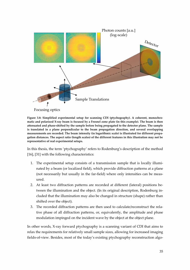
35

In this thesis, the term ‘ptychography’ refers to Rodenburg’s description of the method

[16], [31] with the following characteristics:

1. The experimental setup consists of a transmission sample that is locally illumi-

nated by a beam (or localized field), which provide diffraction patterns at a plane

(not necessarily but usually in the far-field) where only intensities can be meas-

ured.

2. At least two diffraction patterns are recorded at different (lateral) positions be-

tween the illumination and the object. (In its original description, Rodenburg in-

cluded that the illumination may also be changed in structure (shape) rather than

shifted over the object).

3. The recorded diffraction patterns are then used to calculate/reconstruct the rela-

tive phase of all diffraction patterns, or, equivalently, the amplitude and phase

modulation impinged on the incident wave by the object at the object plane.

In other words, X-ray forward ptychography is a scanning variant of CDI that aims to

relax the requirements for relatively small sample sizes, allowing for increased imaging

fields-of-view. Besides, most of the today’s existing ptychography reconstruction algo-

Focusing optics

Sample Translations

Photon counts [a.u.] (log-scale)

Figure 3.8: Simplified experimental setup for scanning CDI (ptychography). A coherent, monochro-

matic and polarized X-ray beam is focused by a Fresnel zone plate (in this example). The beam is then

attenuated and phase-shifted by the sample before being propagated to the detector plane. The sample

is translated in a plane perpendicular to the beam propagation direction, and several overlapping

measurements are recorded. The beam intensity (in logarithmic scale) is illustrated for different propa-

gation distances. The aspect ratio (length scales) of the different features in this illustration may not be

representative of real experimental setups.

36

rithms recover simultaneously not only the object (expression (3.6)) but also the illumi-

nation or probe function (expression (3.5)) which facilitates data acquisition and allows

the use of a variety of diffractive optics for focusing the beam.

The fundamental principles of ptychography are analogous to those of CDI, i.e. the

reconstructed image contrast is given by both intensity and phase modulations of the

incoming wave front according to expression (2.18) and the exit wave is propagated in

free-space to the detector plane that measures its intensity. Before illuminating the

sample, the incoming beam passes through a pinhole or is focused by some type of X-

ray optics that defines the incoming illumination properties, such as size, intensity and

phase. At the sample plane, the electric field of the incoming wave front is defined by

𝜓in or for notation purposes by 𝑃 (as in expression 3.5)). The sample is then translated

in a plane perpendicular to the X-ray beam propagation direction, and different inten-

sity measurements (in the far-field) are recorded at different scanning positions. X-ray

ptychography is not necessarily performed in the focal plane where the illumination

size is small, but often slightly out of focus so that the illuminated area of the object is

large and the number of scanning points can be reduced.

Phase Retrieval in X-ray ptychography

Since its inception by Hoppe, several reconstruction algorithms have been suggested

by different authors to recover the relative phase between diffraction patterns from

adjacent scanning positions. The first ptychographic technique which yielded recon-

structions of non-crystalline specimens was introduced by Bates and Rodenburg and is

known as Wigner-distribution deconvolution [32], [33]. Although this method provides

a closed-form solution to the phase-retrieval problem, it has not been extensively used

besides from some proof-of-principle experiments, mainly due to its high sampling

requirements which limit its practical implementation. For this reason, and since many

different methods (and/or variants) are available in the literature, I introduce only two

of the most predominant iterative algorithms commonly known as Ptychographical

Iterative Engine (PIE) and Difference Map (DM).

Ptychographic Iterative Engine (PIE)

The first iterative algorithm for ptychographical reconstructions was proposed by

Faulkner and Rodenburg (2004) and is known as Ptychographical Iterative Engine PIE

[28], [34], [35]. The PIE algorithm assumes a perfect knowledge of both amplitude and

phase of the two-dimensional probe function, which may be bandwidth-limited, have

infinite spatial extent and/or soft edges [36]. Besides the known probe function and

measured diffraction intensities, the PIE algorithm takes as input an arbitrary guess for

the object function 𝑂[0] that is updated at each iteration according to the following

steps [34], [35]. Assuming the forward model

37

𝐼𝑗(𝒒) = |ℱ{𝑃(𝒓 − 𝑹𝑗) ∙ 𝑂(𝒓)}|2, (3.16)

at the 𝑖th iteration, a new guess of the exit wave 𝜓𝑗[𝑖] is calculated from the current

guess of the object 𝑂[𝑖](𝒓), and the probe function 𝑃 shifted to the scanning position 𝑹𝑗

𝜓𝑗[𝑖](𝒓) = 𝑃(𝒓 − 𝑹𝑗) ∙ 𝑂

[𝑖](𝒓). (3.17)

Analogously to the HIO algorithm, the Fourier constraint is enforced by replacing the

magnitude of the propagated exit wave |Ψ𝑗[𝑖]| by the squared root of the measured in-

tensities

Ψ𝑗[𝑖](𝒒) = ℱ {𝜓𝑗

[𝑖](𝒓)}, (3.18)

𝜓𝑗′[𝑖](𝒓) = ℱ−1 {√𝐼𝑗

meas(𝒒)Ψ𝑗[𝑖](𝒒)

|Ψ𝑗[𝑖](𝒒)|

}. (3.19)

Finally, the object function is updated at the current illuminated area according to

𝑂[𝑖+1](𝒓) = 𝑂[𝑖](𝒓) + 𝛽|𝑃(𝒓−𝑹𝑗)|

max(𝑃(𝒓−𝑹𝑗))

𝑃∗(𝒓−𝑹𝑗)

|𝑃(𝒓−𝑹𝑗)|2+𝛼(𝜓𝑗

′[𝑖](𝒓) − 𝜓𝑗[𝑖](𝒓)). (3.20)

The steps described by equations (3.17) to (3.20) are repeated for all scanning positions

until the whole scanned object area is updated and a new iteration of the algorithm

begins. In (3.20), 𝛽 is a feedback update constant similar to that used in Fienup phase

retrieval algorithms as in (3.8) to (3.10).

In (3.20), the first term |𝑃| max(𝑃)⁄ is a weighting factor that aims to compensate for the

effect of probe intensity variations in the illuminated area. The object function update

is consequently favoured at highly-illuminated areas as opposed to weakly-illuminated

regions where otherwise artefacts or errors would be observed. The second term

𝑃∗ (|𝑃|2 + 𝛼)⁄ removes the contribution of the probe function from the exit wave and

can be seen as a deconvolution‡‡ step by means of a Wiener filter [37]. Please note that a

simple division of the exit wave (or the difference term in (3.20)) by the probe function

would be undefined in regions where |𝑃(𝒓 − 𝑹𝑗)| = 0 , which is avoided in

𝑃∗ (|𝑃|2 + 𝛼)⁄ by including a small constant value 𝛼 in the denominator.

‡‡ The multiplicative relation between the object and probe function corresponds to a convolu-

tion between the Fourier transforms of the probe and object at the detector plane.

38

The illumination overlap constraint is implicitly described by (3.17), since the probe

functions 𝑃(𝒓 − 𝑹𝑗) and 𝑃(𝒓 − 𝑹𝑗+1), at adjacent scanning points partially overlap (as

shown in the example in Figure 3.9Figure ).

The extension of the PIE algorithm for simultaneous reconstruction of the object and

probe function was later proposed by Maiden and Rodenburg (2009) [38] by introduc-

ing expression (3.21) for the probe update function. This algorithm is known as ePIE

and stands for extended ptychographic iterative engine. In ePIE, the probe function up-

date proceeds in a similar fashion as the object update function in (3.20), according to

𝑃[𝑖+1](𝒓) = 𝑃[𝑖](𝒓) + 𝛽𝑃𝑂∗(𝒓+𝑹𝑗)

|𝑂(𝒓+𝑹𝑗)|2+𝛼(𝜓𝑗

′[𝑖](𝒓) − 𝜓𝑗[𝑖](𝒓)), (3.21)

where 𝛽𝑃 has the same role as 𝛽 in (3.20) and may be adjusted to modify the update

step-size. Here, I note that some differences between the expressions in this thesis and

those in the original papers, or following work, may exist. For example, in Maiden and

Rodenburg’s original paper [38] the small constant/regularization term 𝛼 and the

weighting term |𝑃| max(𝑃)⁄ in the object update function are omitted although they

may be required for numerical purposes.

The convergence of this ptychography reconstruction algorithm may be monitored in a

similar way as in CDI phase retrieval, by means of the sum squared error (SSE) be-

7

[rad]Reconstructed Object Phase

Probe Amplitude

Probe Overlap

Figure 3.9: Probe overlap in ptychography data acquisition. On the left: example of a reconstructed

object function (phase) from a catalyst powder in a capillary tube, acquired at the cSAXS beamline

(2004). The scanning positions are marked with a cross symbol, and the dashed circles represent the

probe extent/size at the first 3 scanning positions. The probe amplitude is represented on the top right

(with brightness proportional to the amplitude). The bottom right image superimposes the amplitude

of the probe at the first 3 scanning positions.

39

tween the experimentally measured intensities and those resulting from the squared

Fourier magnitude of the current reconstructed exit wave Ψ𝑗[𝑖] as

𝑆𝑆𝐸[𝑖] =∑ ∑ (𝐼𝑗

meas(𝒒)−|Ψ𝑗[𝑖](𝒒)|

2)2

𝒒𝑗

∑ ∑ (𝐼𝑗meas(𝒒))

2

𝒒𝑗

. (3.22)

Difference Map Ptychography (DM)

Prior to Maiden and Rodenburg’s extension of the PIE algorithm for probe retrieval,

Thibault proposed an iterative scheme for simultaneous object and probe reconstruc-

tion based on Elser’s difference map algorithm [39]. Elser’s difference map algorithm is

a search algorithm that aims to solve constraint-based problems by formulating them

as a set intersection operation in Euclidean space. Although it has been originally de-

signed to solve the missing phase-problem its applications span to other areas such as

protein folding, anagram unscrambling and Sudoku puzzle solving [39].

Generalized Difference Map Algorithm

The following is based on Elser’s description of the difference map algorithm [39]:

The DM algorithm aims to find a solution for 𝑥 in the intersection of two sets 𝐴 and

𝐵 in Euclidean space. The projection operators 𝑃𝐴 and 𝑃𝐵, given an arbitrary input

value for 𝑥, return a point in the constraint sets 𝐴 and 𝐵 respectively, that is closest

to 𝑥. Each 𝑖th iteration of the DM algorithm updates 𝑥 by applying the mapping

operator 𝐷(𝑥) that may be interpreted as an interpolation between the two projec-

tion operators through a parameter 𝛽𝐷𝑀:

𝑥[𝑖+1] = 𝐷(𝑥[𝑖]), (3.23)

𝐷(𝑥) = 𝑥 + 𝛽𝐷𝑀[𝑃𝐴(𝑓𝐵(𝑥)) − 𝑃𝐵(𝑓𝐴(𝑥))], (3.34)

with

𝑓𝐴(𝑥) = 𝑃𝐴(𝑥) −(𝑃𝐴(𝑥)−𝑥)

𝛽𝐷𝑀, (3.35)

𝑓𝐵(𝑥) = 𝑃𝐵(𝑥) +(𝑃𝐵(𝑥)−𝑥)

𝛽𝐷𝑀. (3.36)

Convergence to a fixed point (global minimum) has been only proven for problems

where 𝐴 and 𝐵 are convex sets [113], although this algorithm can be successfully

applied to more difficult problems, such as phase-retrieval, as it has been empirical-

ly shown.

40

Phase-retrieval problems, in particularly ptychography reconstructions, can be ex-

pressed as two intersecting constraints on the exit wave function 𝜓(𝒓) at each scanning

position. According to the forward model in (3.16), the Fourier modulus constraint

enforces compliance to the measured/recorded intensities

𝐼𝑗(𝒒) = |ℱ{𝜓𝑗(𝒓)}|2, (3.22)

while the overlap constraint states that the exit wave at each scanning positions can be

factorized as a probe and object function according to

𝜓𝑗(𝒓) = 𝑃(𝒓 − 𝑹𝑗) ∙ 𝑂(𝒓). (3.23)

In ptychography reconstructions, these constraints are enforced by the distance-

minimizing projections onto constraint sets expressed by the operators 𝑃𝑨 and 𝑃𝑩 that

act in the state vector �� = (𝜓1(𝒓), 𝜓2(𝒓), … , 𝜓𝑁𝑑𝑝(𝒓)) , with 𝑁𝑑𝑝 equal to the number of

acquired diffraction patterns. In each iteration of the DM algorithm, the projection as-

sociated to the Fourier modulus constraint, let us say 𝑃𝑨, consists simply in replacing

the modulus of the exit wave Fourier transform by √𝐼𝑗 while keeping the original

phases:

𝑃𝑨(��): 𝜓𝑗 → 𝜓𝑗𝐹 = ℱ−1 {√𝐼𝑗

ℱ{𝜓𝑗}

|ℱ{𝜓𝑗}|}. (3.24)

In turn, the projection 𝑃𝑩, associated to the illumination overlap, aims to find a solution

for the object and probe function, here represented by �� and ��, that minimizes the dis-

tance

‖�� − ��𝑂‖2= ∑ ∑ |𝜓𝑗(𝒓) − ��(𝒓 − 𝑹𝑗) ∙ ��(𝒓)|

2𝒓𝑗 , (3.25)

subjected to the constraint (3.23). This way:

𝑃𝑩(��): 𝜓𝑗 → 𝜓𝑗𝑂 = ��(𝒓 − 𝑹𝑗) ∙ ��(𝒓). (3.26)

In (3.24) and (3.25), the superscripts ‘𝐹’ and ′𝑂′ stand for the Fourier modulus and

Overlap constraint respectively, in order to distinguish the constrained state vector

from the input state vector ��. According to Thibault [40], minimization of equation

(3.25) does not have a closed-form solution and must be computed numerically, for

which various optimization methods may be successfully and efficiently applied. Thi-

bault suggested the use of a line minimization for (3.25), which reduces (3.25) to the

following system of equations:

��(𝒓) =∑ ��∗(𝒓+𝑹𝑗)𝜓𝑗(𝒓)𝑗

∑ |��(𝒓+𝑹𝑗)|2

𝑗

, (3.28)

41

��(𝒓) =∑ ��∗(𝒓+𝑹𝑗)𝜓𝑗(𝒓)𝑗

∑ |��(𝒓+𝑹𝑗)|2

𝑗

. (3.29)

While this system of equations cannot be decoupled analytically it has been empirically

found that updating the object and probe function with (3.28) and (3.29) in turn (for

different iterations) is an efficient procedure to find a minimum for (3.25).

The convergence behaviour of the difference map algorithm applied to ptychography

reconstructions may be monitored by the sum squared error (3.22) as in the PIE or ePIE

algorithm, but Thibault has additionally suggested the difference map error metric 𝜖

expressed as

𝜖[𝑖] = ‖��[𝑖] − ��[𝑖−1]‖. (3.30)

Having defined the projection operators 𝑃𝑨 and 𝑃𝑩, the reconstruction algorithm fol-

lows the difference map procedure, taking random complex values for the initial

guesses for the object and probe function. In practice it has been observed that the re-

construction convergence is improved by better initial estimates of the object and probe

function. If an initial probe function is not available, it can be either modelled or esti-

mated from the autocorrelation function of the exit wave. The parameter 𝛽𝐷𝑀 in (3.34)

to (3.36) may take any value in the interval [−1,1], and so far, optimal values (for good

reconstructions) have been found empirically for different datasets. Without any prior

information the values 𝛽𝐷𝑀 = ±1 are preferred because this reduces the number of

projection evaluations per iteration. In fact, replacing 𝛽𝐷𝑀 = 1 in (3.34) to (3.36) reduces

the mapping 𝐷(𝑥) to 𝐷(𝑥) = 𝑥 + 𝑃𝑨(2𝑃𝑩(𝑥) − 𝑥) − 𝑃𝑩(𝑥) which is equivalent to

Fienup’s HIO algorithm [39].

Note on other Ptychography reconstruction algorithms

Reconstruction algorithms for phase-retrieval, specifically for ptychography recon-

structions, are currently in continuous development by different research groups. The

description of the PIE, ePIE, and DM algorithms in this thesis was mainly motivated by

historical reasons and by the fact that they have been implemented in the open-source

software package Ptypy [41] currently widely used at synchrotron beamlines. Howev-

er, I found other ptychography reconstruction methods available in the literature

worth mentioning given some particularities associated to each of the different algo-

rithms.

Already in 2008, prior to the extension of the PIE algorithm for probe retrieval, Guizar

and Fienup [42] proposed a non-linear optimization method for simultaneous recon-

struction of the probe and object function with additional refinement of the probe

scanning positions. This method was seen to return superior reconstruction accuracy in

the presence of noise or when the system parameters are inaccurately known.

42

A general alternating minimization algorithm for nonconvex optimization problems

with application to ptychography reconstructions was introduced by Hesse et al. [43]

in 2014 under the name PHeBIE that stands for Proximal Heterogeneous Block Implic-

it-Explicit method. The major highlight of this work is the clear description of the

method’s mathematical framework, proof of convergence to critical points and com-

parison with other existing reconstruction methods.

Recently in 2018, Odstrčil et al. [44] suggested a new iterative least-squares method for

ptychography reconstructions of the object and probe functions. The reconstruction

algorithm is framed as two constrained optimization problems, one in real space and

other in reciprocal space, where the measured intensity data is assumed to be corrupt-

ed by both Poisson and additive white noise (Gaussian). To account for this mixed

noise model, Odstrčil suggested the use of a negative log-likelihood metric as the op-

timization problem cost-function. This approach is similar to the one used for the 3D

ptychography reconstruction algorithm developed during my work, with the main

difference that the forward model is expressed in terms of the diffraction data ampli-

tudes instead of intensities as in my work [45]. Another relevant characteristic of Od-

strčil’s recent reconstruction method is its ability to estimate variations in the probe

function during data acquisition which translates into lower artefacts in the final re-

constructed object function.

Ptychography in inverse space

The ptychography principles (and algorithms) may also be applied in the reciprocal

space in what is known as Fourier ptychography. This technique is often used with

visible light (such as lasers) and with the aid of imaging optics such as lenses. In Fouri-

er ptychography however, the measured intensities in the detector plane correspond to

a real space image, and the “field-of-view” of the reciprocal space is enlarged by means

of a ptychography reconstruction algorithm. The resulting reconstructed real space

image spans the same spatial FOV as in the detector but has increased spatial resolu-

tion when compared with a single measurement [46]–[48].

43

X-ray fluorescence mapping – XRF

X-ray fluorescence (XRF) is a non-destructive spectroscopy technique used to deter-

mine the chemical composition of a sample and their relative elemental concentrations.

The principles of XRF are based on the photoelectric effect and X-ray fluorescence

emission by the sample under investigation upon excitation by an incident high-

energetic X-ray beam§§ as briefly described in Chapter 2.5.

In a conventional XRF experiment, a sample is illuminated and excited by a high-

energy focused X-ray beam. As a consequence, the sample emits X-rays in a broad

spectrum that is recorded by an X-ray fluorescence detector. Each XRF measurement

returns an X-ray spectrum with characteristic peaks and background that carry infor-

mation about the chemical composition (and other external factors) of the sample area

under illumination. X-ray fluorescence maps are finally generated by combining sever-

al XRF spectra measured at different scanning positions. After data acquisition, the

recorded XRF spectra must be analysed and decomposed into the different contribu-

tions from the individual elemental peaks, background and other possible features.

This is often done by fitting a model of the generated intensities by a group of elements

(selected by the user) to the measured spectra via for example a least-squares minimi-

zation approach.

The relationship between elemental concentration and intensity of the emitted X-rays

depends on several factors besides the sample’s composition, including for example

the experimental setup itself. In the mid-1950s, J. Sherman proposed a theoretical mod-

el that describes the relationship between the emitted intensities and elemental concen-

tration that later became the basis for the “fundamental parameters” approach for XRF

calibration [49]. In this thesis I include Sherman’s main remarks under the simplifying

assumptions: a two-dimensional sample of thickness ℎ is illuminated by a parallel and

monochromatic X-ray beam with incoming intensity 𝐼0 with an incident angle of 90°,

i.e. the incident beam is perpendicular to the sample’s surface (see Figure 3.10). Also

for simplification, I will only consider primary fluorescence events and I will mainly

focus on the 𝐾𝛼 X-ray emission of an element with index ‘𝑗’ and mass concentration 𝑤𝑗.

Secondary and tertiary fluorescence occurs when the primary (or secondary) X-ray

fluorescence emission induces characteristic fluorescence events in other elements (or

lower energy shells) of the sample. These effects are often accounted for, in XRF data

analysis, with more advanced models or by means of modelling methods such as Mon-

te Carlo simulation [50].

§§ An electron beam may also be used as incident probe, for which the technique received dif-

ferent names, such as, electron-probe X-ray fluorescence (EP-XRF), energy dispersive X-ray

spectroscopy (EDX), wavelength dispersive X-ray spectroscopy (WDX), among others.

44

The quantitative analysis for mass concentration estimations from fluorescence intensi-

ty measurements is here described in different steps:

First, I introduce the relationship between the incoming beam attenuation and

the X-ray photon absorption by an element with index ‘𝑗’;

Then, the probability for a 𝐾𝛼 photon emission is estimated based on the ab-

sorption jump ratio, transition probability and fluorescence yield;

Finally, the attenuation of the emitted 𝐾𝛼 photons from the sample to the fluo-

rescence detector is taken into account.

The attenuation or absorption of the incoming beam by the sample is described by the

Beer-Lambert law as in expression (2.15), i.e. a sample material with an average linear

absorption coefficient 𝜇𝑠 , attenuates the incoming beam over the X-ray penetration

depth according to

𝐼(𝑧) = 𝐼0e−𝜇𝑠𝑧. (3.31)

The absolute fraction of radiation intensity that is absorbed by an element of thickness

d𝑧 is determined by combining equation (3.31) with its derivative with respect to the

penetration depth 𝑧:

d𝐼

𝐼= 𝜇𝑠d𝑧. (3.32)

However, the radiation may be absorbed by the different elements that constitute the

sample, and only a fraction of it is received by the element with index ‘𝑗’. This fraction

is given by the product of the elemental mass concentration 𝑤𝑗 and the ratio between

the mass absorption coefficient of the element and the sample respectively. Please note,

Sample Translations

XRF Detector

(a) (b)

XRF Detector

Incident beam

Figure 3.10: (a) (Example) of experimental setup for an XRF scanning experiment. A focused X-ray beam

illuminates an area of the sample that consequently emits fluorescent X-rays in all directions. The frac-

tion of the emitted X-rays seen by the detector is defined by the solid angle 𝛀. (b) Relative orientation

between incident beam, sample and XRF detector.

45

that the mass attenuation coefficient is defined as 𝜇/𝜌, and thus equation (3.32) takes

the form

d𝐼𝑗

𝐼= (𝑤𝑗

𝜇𝑗𝜌𝑠

𝜇𝑠𝜌𝑗) 𝜇𝑠d𝑧, (3.33)

that now represents the fraction of the incident radiation intensity that is absorbed by a

specific element ‘𝑗’ in an infinitesimal thickness d𝑧. In equation (3.33), 𝜌𝑠 and 𝜌𝑗 repre-

sent the mass density of the sample and the element ‘𝑗’ respectively.

The radiation absorbed by a specific element can still result in several electron transi-

tions between the different energy shells of the atom (besides the 𝐾𝛼 emission). To ac-

count for this, one often relies on the excitation factor 𝑄𝐾𝛼 that in turn is defined as the

product of the probabilities of three main events:

The probability of an electron to be ejected from a K-shell rather than another

(shell);

The probability for a 𝐾𝛼 emission (L-K transition) rather than 𝐾𝛽 (M-K transi-

tion) or other possible K lines;

The probability for the ejection of an Auger electron rather than 𝐾𝛼 emission.

The probability of an electron to be ejected from a K-shell rather than an L- or M-shell

is expressed by the absorption jump factor (or ratio) 𝐽𝐾:

𝐽𝐾 =𝑟𝐾−1

𝑟𝐾, (3.34)

(a) (b)

Figure 3.11: (a) Linear absorption coefficient (and imaginary decrement of refractive index) for a

Cu2ZnSnS4 sample around the Zn characteristic K-edge. (c) Fluorescence yields for the 𝑲𝜶 and 𝑳𝜶 lines

emission as function of the material atomic number, based on semi-empirical analytical expressions

from Hubbell [114].

46

where 𝑟𝐾 is the K-shell absorption jump defined as the ratio between the linear absorp-

tion coefficients at the K absorption edge as illustrated in Figure 3.11a:

𝑟𝐾 =𝜇max

𝜇min. (3.35)

Second, the probability for a 𝐾𝛼 emission rather than other possible K-lines is given by

a transition probability 𝑔𝐾𝛼 :

𝑔𝐾𝛼 =𝐼(𝐾𝛼)

𝐼(𝐾𝛼)+𝐼(𝐾𝛽). (3.36)

Finally, the probability for a 𝐾𝛼 radiation emission rather than the ejection of an Auger

electron is dictated by the fluorescence yield 𝜔𝐾. The fluorescence yield for the 𝐾𝛼 and

𝐿𝛼 lines of some materials is represented in Figure 3.11b.

The absorption jump ratio, transition probability and fluorescence yield may be de-

termined experimentally or based on theoretical models. The resulting excitation factor

is then:

𝑄𝐾𝛼 = 𝐽𝐾𝑔𝐾𝛼𝜔𝐾 =𝑟𝐾−1

𝑟𝐾

𝐼(𝐾𝛼)

𝐼(𝐾𝛼)+𝐼(𝐾𝛽)𝜔𝐾. (3.37)

The fluorescent radiation generated by the infinitesimal volume is still attenuated by

the sample through its path back to the detector. If one neglects any other form of at-

tenuation (as for example attenuation by the air between the sample and detector) the

fraction of radiation that reaches the detector is given by

exp [−𝜇𝑠,𝐾𝑗𝑧

cos (𝜙𝑑) ]. (3.38)

The sample’s linear absorption coefficient is represented in (3.38) by 𝜇𝑠,𝐾𝑗 to distin-

guish it from 𝜇𝑠 in (3.31), as the first is calculated for an excitation energy equal to the

emitted fluorescent radiation energy, whereas the second is calculated for the excita-

tion energy of the incoming beam.

Besides the aforementioned remarks, the fluorescent radiation is emitted uniformly in

all directions over a solid angle of 4𝜋 sr (as represented by the green sphere in Figure

3.10) although only a fraction of it (Ω/4𝜋) is seen by the XRF detector. Taking all this

into account, the primary 𝐾𝛼 fluorescent radiation from an element ‘𝑗’ of thickness d𝑧 is

given by

d𝐼𝑗 =Ω

4𝜋𝐼0e

−𝜇𝑠𝑧 (𝑤𝑗𝜇𝑗𝜌𝑠

𝜇𝑠𝜌𝑗) 𝜇𝑠𝑄𝐾𝛼 exp [−𝜇𝑠,𝐾𝑗

𝑧

cos(𝜙𝑑) ] d𝑧. (3.39)

Integrating (3.39) with respect to 𝑧 through the whole sample thickness (𝑧 = [0, ℎ]) re-

sults in

47

𝐼𝑗 =Ω(𝐼0𝜔𝑗𝜇𝑗𝜌𝑠𝑄𝐾𝛼)

4𝜋𝜌𝑗(𝜇𝑠+𝜇𝑠,𝐾𝑗 cos(𝜙𝑑)⁄ )

(1 − exp [−ℎ (𝜇𝑠 + 𝜇𝑠,𝐾𝑗 cos(𝜙𝑑)⁄ )]). (3.40)

Equation (3.40) can now be used as a forward model to estimate the emitted intensity

(or photon counts) by a specific element, according to the previously mentioned as-

sumptions. This forward model is then used by some type of optimization algorithm in

order to match the experimentally measured intensities (for all detectable elements), so

that the mass concentrations 𝜔𝑗 can be determined. If the measured sample consists of

a stack of layers of different materials, the forward model in (3.40) must be extended to

include additional self-absorption events that may occur at the different layers (with

different linear absorption coefficients and thicknesses).

X-ray fluorescence spectroscopy has been widely used in combination with scanning

electron microscopy. Electron beams are often easier to control and manipulate (using

magnetic and electric fields), and thus may yield smaller probe sizes and higher spatial

resolutions, with suitable high fluxes. On the other hand, X-rays have higher penetra-

tion depths when compared to electrons (see Figure 3.12) and thus are not limited to

surface measurements. Besides, X-ray induced XRF spectra have higher elemental sen-

sitivity, usually a lower Bremsstrahlung or continuous background and do not require

the sample to be conductive and electrically grounded during measurement.

x [µm]

y [µm] Electrons X-raysy [µm]

x [µm]x [µm]

y [µm] Electrons X-raysy [µm]

x [µm]

Figure 3.12: Comparison between the interaction volumes of an electron and X-ray beam incident on a

kesterite (Cu2ZnSnS4) substrate. An incoming beam of 10.4 keV (electrons or photons) reaches the sub-

strate surface (𝒚 = 𝟎) with a diameter of 𝟏𝟎𝟎 nm, scatters and is absorbed or transmitted by the sample.

Backscattered particles (electrons or photons) are represented by yellow lines whereas all remaining

trajectories are represented in blue. The end point of a trajectory corresponds to the full absorption of

an electron or photon. For identical energies, the interaction volume for an electron beam gets confined

to penetration depths lower than 𝟏 𝛍𝐦, whereas for X-rays the beam is almost fully transmitted through

the whole sample. A total of 1000 trajectories were simulated using the Monte Carlo model of the open-

source software pyPENELOPE [115].

48

X-ray beam induced current mapping – XBIC

Beam-induced current techniques have been successfully applied to the investigation

of local electrical properties of semiconductor materials. Their fundamental principle

relies on the measurement of the electric current generated by a specimen upon excita-

tion by an optical (OBIC or LBIC), electron (EBIC), or X-ray beam (XBIC).

In a wider context, X-ray beam induced current techniques may include all different

forms of X-ray detection in which the measured current is, at a first approximation,

proportional to the number of absorbed X-ray photons. For example, an X-ray (absorp-

tion) detector consisting of a scintillator and a CCD (charged-coupled device) can be

said to exploit the XBIC principle during data acquisition. Nevertheless, the term XBIC

is generally used for experiments, in which the specimen acts as detector itself, i.e., the

measured current arises from electron-hole pairs generated in the sample upon X-ray

excitation. As any beam-induced current technique, XBIC is a powerful tool for the

study and characterization of solar cells. The technique’s full potential is realized when

XBIC is combined and correlated with XRF measurements, from which a relationship

between the charge collection efficiency (CE)and the specimen’s elemental composi-

tion can be determined. The charge collection efficiency quantifies the probability of

converting photons into electric current and plays a fundamental role in solar cells en-

gineering, where losses due to recombination (1 − CE)should be minimized.

In 2000 H. Hielsmair, et al. [51] proposed, with proof of principle, the use of XBIC for

the investigation of crystalline silicon solar cells. Their main motivations were the

higher penetration depth of X-rays when compared to electrons (EBIC) and the possi-

bility to simultaneously acquire XRF data with sufficiently high sensitivity to detect

trace elements and microdefects in fully functional devices. In the last few years, XBIC

measurements have been extended from silicon to thin-film solar cells such as CIGS

[52], CdTe [53], organic photovoltaics (OPV) [54], perovskite [55] and kesterite (see

Chapter 5).

49

The experimental setup and strategy for XBIC data acquisition follows the same prin-

ciples of a scanning method such as XRF, in the sense that a highly focused X-ray beam

excites a localized area of the specimen, from where the signal is measured. The sample

is then moved to a new scanning position and the measurements are repeated until a

full two-dimensional map representative of a region of interest is acquired.

While in XRF one exploits the emitted fluorescent radiation resulting from the ejection

of an electron from an atom (photoelectron), in XBIC the recorded signal is given by

measurements of the current generated by the ejected electrons. XBIC distinguishes

from other photoelectron measurement techniques, such as X-ray photoemission elec-

tron microscopy (XPEEM) or photoelectron spectroscopy (XPS), in the way the electric

current is measured. In XPEEM, or other analogous methods, the electrons emitted

from a surface are directly measured (see Figure 3.13 left) whereas in XBIC the elec-

trons are measured indirectly by exploiting the semiconductor properties of a p-n junc-

tion***. The circuit schematics in Figure 3.13 left, shows an example of an experimental

setup for the measurement of the total electron yield (TEY). After photoexcitation, and

electron emission, the sample surface becomes positively charged and new electrons

flow from a grounded connection to restore charge neutrality in the sample. In this

*** A p-n junction is one of the simplest ways to create a semiconductor device, by joining a p-

type (positive) material with excess of holes with an n-type material with excess of electrons. A

p-n junction diode only allows current to flow in one direction, i.e. electrons flow easily through

the junction from the n- to the p-type material, and the opposite for the holes.

n

p

-

A

n

p

-

-+

A

TEY XBIC

Figure 3.13: Experimental setups for TEY (left) and XBIC (right) measurements. In TEY, photoelectrons

ejected from the layer where X-rays are incident, locally recombine or are replaced by new electrons

from a grounded connection. The replacement current is measured between the exit-layer and the

ground thus representing the sample’s total electron yield. In XBIC, the replacement current is instead

measured between the two terminals of the p-n junction, and thus only charge carriers dissociated at

the p-n junction contribute to the measured current.

50

case, the replacement current is a measure of the ejected electron current, which after

normalization with respect to the incident photon flux returns the TEY.

For XBIC measurements on solar cell devices (or other type of semiconductor material),

the setup on Figure 3.13 right must be used instead [56]. The incoming X-ray beam may

hit either the p- or n-type material, as long as the incident layer is electrically ground-

ed, and the current is measured between the p- and n-type materials. This way, elec-

trons ejected from the top layer (where the X-rays are incident) are quickly replenished

by the electrically grounded connection but do not contribute to the measured current.

In fact, any electron or hole generated in the p- and n-type layers are prone to recom-

bine since the p-n junction limits one of the charge carriers’ mobility through the junc-

tion. However, electron-hole pairs generated by the X-ray photons in the absorber lay-

er, as analogously happens with visible light in standard solar cells operation, diffuse

to the p- and n-type semiconductors, generating a potential bias. The electric current

measured by closing the circuit between the two semiconductors is then only depend-

ent on the generated charge carriers in the absorber layer and is representative of the

device’s charge collection efficiency (CE) [57]. In turn, the charge collection efficiency is

defined as the ratio between the number of collected ( 𝑁𝑒−/ℎ+coll ) and the number of gen-

erated ( 𝑁𝑒−/ℎ+gen

) electron-hole pairs (𝑒−/ℎ+) as

CE = 𝑁𝑒−/ℎ+coll

𝑁𝑒−/ℎ+gen . (3.41)

In the photovoltaic community, the charge collection efficiency is often interpreted

from external (EQE) and/or internal quantum efficiency (IQE) measurements that are

available with standard laboratory equipment with absolute errors on the order of 1%.

The EQE and IQE describe the ratio between the number of collected electron-hole

pairs and the number of incident (𝑁𝑝in) or absorbed (𝑁𝑝

abs) photons respectively:

EQE = 𝑁𝑒−/ℎ+coll

𝑁𝑝in , (3.42)

IQE = 𝑁𝑒−/ℎ+coll

𝑁𝑝abs . (3.43)

Solar cells usually operate in the visible part of the electromagnetic spectrum, where

the generation of more than one electron-hole pair per incident photon can be consid-

ered negligible. Under this condition (visible light), the number of generated charge

carriers may be approximated to the number of absorbed photons so that 𝑁𝑒−/ℎ+gen

≈

𝑁𝑝abs. Also, under the assumption of null transmittance, i.e. the incident light is either

51

absorbed or reflected, the number of absorbed photons can be approximated by

𝑁𝑝abs ≈ 𝑁𝑝

in(1 − 𝑅), where 𝑅 represents the device’s reflectance, or if preferred, the frac-

tion of light that is not absorbed. This way, under the assumption of photoexcitation

with visible light:

CE = 𝑁𝑒−/ℎ+coll

𝑁𝑒−/ℎ+gen ≈ IQE =

𝑁𝑒−/ℎ+coll

𝑁𝑝in(1−𝑅)

=EQE

(1−𝑅). (3.44)

However, in the X-ray part of the electromagnetic spectrum, the approximations in

(3.44) do not hold, mainly because a high-fraction of the X-rays is fully transmitted

through the sample and the emitted fluorescent radiation may promote a cascade of

photoexcitation events. The number of generated charge carriers is then estimated from

the incident photon flux by means of a correction factor 𝐶 that accounts for the absorb-

er layer absorptance and the number of generated electron-hole pairs per absorbed

photon. This way, the charge collection efficiency under excitation by X-rays, here de-

noted by CEX is then expressed as

CEX = 𝑁𝑒−/ℎ+coll

𝑁𝑒−/ℎ+gen ≈

𝑁𝑒−/ℎ+coll

𝐶∙𝑁𝑝in . (3.45)

For proper quantification of XBIC signals, the correction factor 𝐶 must be estimated

taking into account X-ray absorption and secondary particle interactions. For this rea-

son calculations based on the Beer-Lambert’s attenuation law alone do not suffice and

more complex models, based for example on Monte Carlo simulations, must be used

instead. Although Stuckelberger et al. [56] suggested a method for estimating the cor-

rection factor 𝐶, based on the properties of the sample and incoming X-ray beam, as

pointed out by the same authors, absolute/quantitative CEX measurements with rela-

tive low errors are still out of reach with current experimental methods and equipment.

Errors in XBIC measurements are mostly attributed to the lack of calibrated X-ray de-

tectors installed at synchrotron beamlines and uncertainties in the sample layer thick-

nesses. Nonetheless, relative/qualitative maps of CEX, normalized to 100%, still provide

useful information and highlight local differences in charge collection efficiency within

the same specimen with high spatial resolution.

52

3.3 Challenges in high-resolution imaging

In this chapter I introduced the main X-ray imaging and mapping techniques that I

have worked with during my PhD studies. The described methods exhibit unique im-

aging characteristics that are of special relevance for the structural, chemical and elec-

trical characterization of solar cell devices, currently a hot research topic at DTU, and

more specifically at DTU Energy.

However, the applicability of these techniques, for example for characterization of the

active layer of organic photovoltaics, has been mainly restricted by the obtained spatial

resolutions currently provided by most synchrotron beamlines. Whereas the spatial

resolution of coherent diffractive imaging techniques such as full-field CDI and

ptychography is mostly diffraction-limited, other factors such as the degree of coher-

ence of the illumination wave front, and the possibility for induced radiation damage

also have meaningful contributions. On the other hand, in mapping techniques such as

XRF and XBIC the obtained spatial resolution is a function of the distance between two

adjacent scanning points and the size of the illumination function, or if preferred, the

interaction volume between the incoming X-rays and the sample.

The extension of ptychography imaging to 3D, by means of tomographic principles

(see Chapter 4), requires additional computational operations such as phase-

unwrapping, background normalization, tomographic alignment and reconstruction. If

these are not carried out satisfactorily, they may also be a source of additional artefacts

or result in degradation of the final tomogram resolution.

In the last three years, most of the work developed during my PhD was devoted to the

improvement of the ultimate high-resolution of different X-ray imaging techniques by

numerical methods. This problem was addressed in three independent but related

tasks:

1. We introduced an automated tomographic alignment algorithm [9] with appli-

cation to phase-contrast (CDI or ptychography) tomography, which includes a

self-consistent iterative refinement of the translational and angular alignment

parameters. The method we proposed was successfully applied to simulated

and real datasets and suggested that the final three-dimensional spatial resolu-

tion of a reconstructed tomogram can be improved by a three-dimensional

alignment of the reconstructed projections. During our investigations we have

seen our alignment method to fail on datasets with heavily wrapped projections

and in the presence of phase residues (see Phase-Wrapping), that should and can

be avoided or reduced by proper design of the sample and experimental setup.

So far, for good datasets, the main limitation of our method’s implementation

53

and performance is its requirement for large memory (RAM) and graphic pro-

cessor units (GPU). Fortunately we are currently observing a fast expansion and

quick development of these computational resources that will certainly fulfil

our needs in the near future. A MATLAB implementation of our tomographic

alignment and reconstruction method was made publically available and can be

accessed through reference [58].

2. As part of a collaboration project with MAX-IV laboratory, under the IN-

TERRREG project, we developed a numerical method for resolution enhance-

ment of “STXM-type” images by means of a deconvolution with the illumina-

tion intensity function. The proposed method is further described in Resolution

Enhancement of STXM-type techniques by probe deconvolution.

3. We introduced a new numerical method that extends ptychography reconstruc-

tions to three dimensions. Our reconstruction algorithm described in reference

[45] iterates directly between a three-dimensional function representing the re-

fractive indices of a sample and the intensities of coherent diffraction patterns

measured at different scanning and angular positions. By exploiting data re-

dundancy between different tomographic angles in a single reconstruction vol-

ume, three-dimensional phase-retrieval/reconstruction algorithms have proved

to relax the requirements for illumination overlap during data acquisition. Be-

sides the possibility for faster acquisition times, the scanning geometry can also

be optimized for a uniform dose distribution on the sample, which in turn is

not only beneficial from a numerical point of view during data reconstruction

but also decreases the possibility of radiation damage on the sample. So far, the

application of our reconstruction algorithm relies on the precise knowledge of

the relative positions between the beam and the sample at different rotation an-

gles, which is often only fully available after tomographic alignment of the re-

constructed projections. Today, interferometric systems for active control of the

sample movement can achieve sub-10 nm precision but are unable to track large

sample movements necessary when rotating the sample with accuracies better

than ~100 nm. The route for higher-resolution phase-contrast tomography (or

coherent diffraction imaging) is thus dependent on the continuous develop-

ment of interferometric alignment systems combined with ever-increasing

computational resources, new reconstruction algorithms, and new generation

synchrotrons. A MATLAB implementation of this reconstruction tool is availa-

ble online and can be accessed through the DOI: 10.6084/m9.figshare.6608726.

Different approaches to improve the spatial resolution of CDI reconstructions have

already been proposed in the literature by various research groups. For example, in

2011 Maiden et al. [59] suggested the possibility to extrapolate the recorded diffraction

54

patterns intensities beyond the detector’s aperture during ptychography reconstruction

using a modified version of the ePIE algorithm. This superresolution technique has

shown promising results and reported the ability for large increases in resolution over

3 − 5 times, without the acquisition of additional data or introduction of noise.

CDI techniques often assume full spatial (transverse) and temporal (longitudinal) co-

herence of the incident X-rays and thus small deviations from the ideal setup can pre-

vent the reconstruction algorithm to fully converge. Based on Wolf’ coherent-mode

decomposition model [60], [61], different authors proposed modifications to the con-

ventional full-field CDI reconstruction algorithms to account for partial transverse [62]

and longitudinal [63] coherence of the illumination source. Later, Thibault and Menzel

[64] applied the same principle of multi-mode probe decomposition to ptychography

reconstruction algorithms which consequently relaxes the coherence requirements of

the experiment, allowing for higher fluxes and shorter exposure times, and improves

the final reconstruction quality by minimizing reconstruction artefacts.

Coherent diffraction patterns, especially those from a parallel X-ray beam and recorded

in the far-field, are often significantly brighter at their centre and may have very low

(or null) counts at large scattering angles that are associated with the smaller scatter-

ers/features in the sample. In order to increase the reconstructed spatial resolution one

must access and measure with sufficient statistics the high frequency information en-

coded in high scattering angles, in the outer parts of the detector. Higher counting sta-

tistics can be obtained by increasing the exposure time, but because of the large dy-

namic range of intensities in the detector this may cause saturation of lower diffraction

orders. Alternatively, as demonstrated by Li et al. [65], an optical static diffuser mount-

ed close to the specimen can be used to spread the recorded intensities uniformly over

all detector pixels and extend the angular range of the recorded intensities. Besides,

any form of illumination function becomes highly structured after passing through a

diffuser, a characteristic that is known to be favourable during ptychography recon-

struction and for decoupling the different illumination modes.

As experimental setups for data acquisition are becoming more stable, light sources

more brilliant and coherent, and reconstruction algorithms more robust, CDI methods

will most likely reach the spatial resolution limit, imposed by the coherent properties

of the illumination source or by the radiation damage on the sample [66].

55

Coherence requirements

Despite the fact that numerical algorithms for CDI and ptychography reconstructions

that account for partial illumination coherence exist, I found relevant to highlight the

theoretical limitations on the spatial resolutions of coherent diffractive imaging meth-

ods. In real experimental setups, the incoming X-ray beam deviates from the ideal de-

scription of a plane wave in two main aspects: the beam is not fully monochromatic

and its propagation direction is not perfectly well defined. Associated twith these fea-

tures are the concepts of longitudinal 𝐿𝐿 and transverse 𝐿𝑇 coherent lengths respective-

ly defined as

𝐿𝐿 =𝜆2

Δ𝜆, (3.46)

𝐿𝑇 =𝜆𝐿

𝑊, (3.47)

where Δ𝜆 represents the wavelength bandwidth measured at FWHM, 𝐿 the distance

from the sample to the detector and 𝑊 the width of the object (in CDI) or illumination

function at the object plane (in ptychography). The coherence and sampling require-

ments for optimum results in diffractive imaging are succinctly described in the review

work by Spence et al. [67]. The Nyquist-Shannon sampling criterion for diffraction pat-

terns intensities was already mentioned in the section of Coherent Diffraction Imag-

(a) (b)

Figure 3.14: Graphical representation of the longitudinal (a) and transverse (b) coherence lengths. (a)

two plane waves are initially in phase and propagate in the same direction but with different wave-

lengths. Consequently, their phase evolves differently and after a propagation distance equal to the

longitudinal coherence length 𝑳𝑳 the two waves are out of phase by a factor of 𝝅. (b) two plane waves,

here represented by their wave fronts/crests, with the same wavelength and initial phase propagate in

different directions, defined by the divergence angle 𝚫𝜽 ≈𝑾 𝟐𝑳 = 𝝀 𝟐𝑳𝑻⁄⁄ . Because the waves propa-

gate with different directions, their relative phase is different in each point on the wavefront. The

(transverse) distance or coherence length is then the distance along a wavefront between points that are

in-phase and out-of-phase.

56

ing, and as explained imposes a maximum size on the specimen for full-field CDI. This

same requirement translates into a maximum size of the probe function at the object

plane for ptychography defined as

𝑊 ≤𝜆𝐿

2𝑑ps. (3.48)

In order to avoid overlap between different diffraction orders in the same pixel of the

detector, under the paraxial approximation, the longitudinal and transverse coherence

lengths must obey:

𝐿𝐿 ≥ 𝑊(2𝜃)max, (3.49)

𝐿𝑇 ≥ 2𝑊. (3.50)

The spatial resolution in CDI is dependent on the sample properties and thus a simple

relation between resolution and coherence lengths is not well defined. However we

can establish these relationships in terms of the object and reconstructed pixel/voxel

sizes. Recalling expression (3.12) and the oversampling criterion, the maximum scatter-

ing angle (2𝜃)max relates to the finest spatial frequency of the object by (2𝜃)max =𝜆

2𝑟𝑝𝑠.

Taking this, and combining (3.46) and (3.47) with (3.49) and (3.51) returns

Δ𝜆

𝜆≤2𝑟𝑝𝑠

𝑊, (3.51)

𝑊 ≤ √𝜆𝐿

2, (3.52)

which impose a maximum relative wavelength bandwidth and size for the object or

illumination function (at the object plane).

Phase-wrapping and Phase residues

Although not directly related to limitations in resolution, the presence of phase-

wrapping in the reconstructed phase of the complex object can introduce challenges

and artefacts during tomographic reconstruction. Because phase-retrieval algorithms

are insensitive to constant phase offsets and the periodic nature of phase signals, the

phase of the reconstructed object is only known modulo 2𝜋, commonly represented in

a [−𝜋, 𝜋] range. Phase unwrapping is possible using numerical methods, such as the

two-dimensional Goldstein unwrapping algorithm [68] or Volkov’s method [69], but

may be unfeasible in the presence of noise, reconstruction artefacts or aliasing due to

undersampling of the phase, i.e. the phase difference between two adjacent pixels is

larger than 𝜋. In the presence of these or other sources of errors, a closed-path integral

around a pixel of the phase image may be different than zero as expected. To these

57

points we give the name of phase residues or more specifically, “positive residue charge”

if the integral returns +2𝜋, or “negative residue charge” if the integral is equal to −2𝜋.

In the datasets I worked with during my PhD studies, the most predominant source of

phase residues was associated with sharp phase transitions that occur at edges between

two materials (or background) with different contrast. As an example, Figure

3.15Figure shows the ptychography reconstruction (phase) of an organic solar cell

with phase wrapped areas and phase residues. The high contrast between the materials

that compose the active layer (PC70BM:P3HS) and the electrodes (Cu and ZnO) is re-

sponsible for large phase transitions at their interface that may not be representable in

a single pixel and thus result in a phase residue. Consequently phase-unwrapping be-

comes challenging or introduces artefacts when conventional algorithms are used, that

propagate further to three dimensions after tomographic reconstruction. To avoid or

mitigate these adverse effects, without changing the composition of the sample system,

one could in principle apply any of the following suggestions:

Phase wrapping can be simply avoided by setting the specimen’s thickness so

that all phase-shifts through the object are smaller than 2𝜋†††, or alternatively

∫𝛿(𝑥, 𝑦, 𝑧, 𝑘)d𝑧 < 𝜆. Here I write 𝛿 as function of the spatial coordinates and

wave vector to highlight its dependency on the incoming illumination energy.

††† Here it could be argued that if air (background) is taken as a reference value for the phase

(equal to zero), the maximum admissible phase-shift on the sample is 𝜋 and values larger than

this will result in wrapped areas.

5 µm

(a) (b) (c) (d)

1 µm 1 µm 1 µm

Figure 3.15: Effect of phase residues in phase unwrapping. (a) Phase-contrast projection of an organic

solar cell with a PC70BM:P3HS bulk heterojunction, acquired at the cSAXS beamline with 6.2 keV

incoming beam and reconstructed pixel size of 11.5 nm. (b) Location of the phase residues (red circles)

in a zoomed area of the specimen with phase wrapping. (c) Volkov’s unwrapping method is not path-

dependent but the presence of phase residues results in artefacts that extend beyond the problematic

area. (d) Goldstein’s branch-cut unwrapping method is able to handle phase residues as long as positive

and negative residue charges can be paired. Otherwise, Goldstein’s method is not robust and becomes

path-dependent as the example shows: In this example the unwrapping procedure started at the top left

corner of the image and thus all points below and at the right of a phase residue are affected by a

strong offset which results in the darker rectangular region in (d).

58

Sharp phase transitions may be reduced and spanned to several pixels by in-

creasing the spatial resolution of the reconstructed projections. This can be

achieved, for example, by reducing the reconstructed pixel size by appropriate

selection of the parameters in equation (3.14). Increasing data redundancy may

also provide additional constraints during reconstruction and decrease the

number of observed artefacts and phase residues.

Although phase residues are mostly located at interfaces, their effect may extend

to a few voxels in each layer of the reconstructed tomogram. If phase residues

cannot be avoided with the available spatial resolution, one may alternatively

increase the height of the layers of interest and aim to guarantee a significantly

wide field-of-view that is not affected by such artefacts.

Radiation damage and X-ray dose

New fourth-generation synchrotrons and free-electron lasers (FEL) are continuously

under development and will progressively deliver X-ray beams with a superior degree

of coherence and significant fluxes. When the coherence properties of the beam are no

longer a limitation to the reconstructed image resolution, this will most likely be re-

stricted by radiation damage suffered by the sample. Long exposures to high-energetic

radiation may lead to different dissociation mechanisms, and eventually cause damage

to the sample, changing its micro- and nanostructure and preventing the visualiza-

tion/reconstruction of its smallest features. For this reason, X-ray imaging experiments

should simultaneously fulfil the minimum required dose for imaging and the maxi-

mum tolerable dose before “unacceptable degradation” of the sample.

Whereas the minimum required dose for imaging can be estimated from statistical cal-

culations such as Rose’s criterion [70], based on the signal-to-noise ratio, critical dose

and desired image contrast, the maximum tolerable dose on the other hand must be

inferred from experimental or simulation results. Howells et al. [66] predicted that the

best achievable resolution for an X-ray diffraction experiment, based on the contrast

between water and a protein is about 10 nm, and suggested that resolutions lower than

1 nm are unlikely even for heavy/radiation-hard materials. Based on their own meas-

urements, and other compiled results from the literature, Howells et al. suggested an

empirical simple linear relationship between maximum allowed dose and resolution

equal to 1.0 × 108 Gy/nm (Gray per nanometer of resolution).

Radiation damage effects can be mitigated in different ways, for example, by perform-

ing experiments at cryogenic temperatures, or by reducing the required dose (for a

given resolution) by means of contrast enhancing agents/strategies. When performing

X-ray tomographic experiments one may additionally optimize the scanning geometry

so that the radiation dose is equally distributed through the different voxels of the ob-

59

ject. In tomography the required dose can be further decreased and distributed (frac-

tioned) over the different projection angles as suggested by the dose fractionation the-

orem. This fundamental theorem introduced by Hegerl and Hoppe [71], and later veri-

fied by McEwen et al. [72] states that three-dimensional reconstructions require the

same integral dose as a single two-dimensional projection image for the same level of

statistical significance. A practical implication of this theorem is that “a statistically

significant 3D reconstruction can be obtained from projections which are not statistical-

ly significant at the limiting resolution” as pointed out by McEwen et al. [72]. Conse-

quently, three-dimensional phase-retrieval and tomographic reconstruction algorithms

as the one in [45], have the possibility to decrease acquisition times and radiation dos-

es, further increasing the limits of maximum obtainable resolution.

Resolution Enhancement of STXM-type techniques by probe deconvolution

The resolution in STXM-type techniques is primarily defined by the focal spot size of

the X-ray beam, whereas mechanical instabilities or drifts due to thermal effects dis-

play minor contributions. The technological advances in X-ray optics, noticeably in

refractive optics such as Fresnel Zone plates, have allowed increasingly smaller focus

sizes that will further enjoy the anticipated coherence of new synchrotron or FEL facili-

ties. The resolution in STXM imaging is in fact approaching competitive values to co-

herent diffractive imaging methods with reported resolutions of 15 nm in the soft X-ray

regime [73]. Furthermore, numerical methods can be used to enhance the spatial reso-

lution of the acquired images, by modelling the interaction between the sample and the

beam based on a priori knowledge of the illumination function. CDI methods such as

ptychography and its variants, available at high coherent sources, allow the reconstruc-

tion of the illumination function while simultaneously measuring a specimen. When

measurements are performed out of focus, propagation methods such as those de-

scribed in Chapter 2.6 can be further used to propagate and characterize the beam in-

tensity at its focal spot.

The performance of numerical algorithms, such as those based on “probe deconvolu-

tion”, is however mostly realized when the distance between two neighbouring scan-

ning positions is significantly smaller than the probe size. This condition is especially

relevant and verified in experiments where simultaneous X-ray ptychography and X-

ray fluorescence measurements are conducted. In these cases, the resolution of XRF

maps is mostly compromised by the large overlap between illuminations in different

scanning positions as is necessary for successful ptychography reconstructions and

may significantly benefit from further deconvolution data analysis. The deconvolution

of X-ray fluorescence maps using a reconstructed illumination function from

ptychography measurements has already been proposed and demonstrated in the lit-

erature, for example, by the work of Deng et al. [74], [75] with frozen-hydrated biologi-

60

cal specimens, where the spatial resolution of the measured fluorescence maps was

improved by a factor of 2. However, in their same work, the authors pointed out some

of the limitations of XRF deconvolution by the Wiener-filter deconvolution method [37]

as it requires additional knowledge of the spatial frequency distribution of the signal

and noise power. Besides, direct deconvolution methods rely on the application of

Fourier transforms that sample the acquired image in a uniform Cartesian grid. Alt-

hough the first demonstration of this method [74] was successfully done using a con-

tinuous-motion or fly-scan ptychography setup (with a uniform Cartesian scanning

grid), fly-scan data acquisition is not limited to regular grids and may take complex

scanning geometries so that the dwell time during the scanning motion can be mini-

mized [74], [76]–[78]. Just as importantly, uncertainties in the scanning positions and

variations in the illumination function during data acquisition posed additional chal-

lenges for probe deconvolution of XRF maps by Wiener-filter deconvolution [74].

On the other hand, numerical algorithms for image deconvolution based on iterative

methods have the possibility to account for specific noise models and include addi-

tional regularizations and constraints to improve the reconstructed image quality [79],

[80]. Motivated by this, during my PhD project we developed a method for enhancing

XRF maps from combined ptychography measurements, based on an optimization

problem that we solve by four analogous but different algorithms. This work was de-

veloped in collaboration with the NanoMAX beamline at MAX IV laboratory under the

EU project: MAX4ESSFUN Cross Border Network and Researcher Programme. The

developed tool was implemented in both MATLAB and Python and is available online

on NanoMAX GitHub repository under the URL

https://github.com/alexbjorling/nanomax-analysis-utils/tree/fmre.

Iterative deconvolution of XRF maps

The process of sampling a signal by a kernel function wider than its sampling period is

mathematically expressed by a convolution operation between the sampled signal and

a point spread function (PSF). As the measured XRF maps are proportional to the in-

coming X-ray beam intensity, the point spread function can in this case be described by

the intensity of the recovered probe function PSF = |𝑃(𝑥, 𝑦)|2. Iterative methods for

image deconvolution are already well established in the literature but implicitly as-

sume that the blurred image and PSF are expressed in the same grid, or in other words

that the data is not sparse. While the “resolution” of the illumination function recov-

ered by ptychography equals the reconstructed pixel size (equation (3.12)), the XRF

maps are expressed in a grid of lower resolution, equal to the distance between neigh-

bouring scanning points. To account for this, our method interpolates the XRF maps to

the ptychography image resolution at each iteration, facilitating also additional analy-

sis between both datasets. Since the process of convolution and sampling can be de-

61

scribed uniquely by linear operations in Euclidean space I have decided to formulate

the following mathematical models in terms of matrices and vectors operations mainly

due to its simple terminology. However our final implementation relied on functions

operators for a faster performance. In the following paragraphs, matrices or two-

dimensional arrays are represented by uppercase boldface letters, vectors by italic low-

ercase boldface letters and constants with plain italic letters.

Forward model description

Let 𝐗 ∈ ℝ𝑁×𝑀 and 𝐁meas ∈ ℝ𝑛×𝑚 represent a solution for the enhanced fluorescence

map (that we aim to reconstruct), and the measured fluorescence map respectively,

described in a 𝑁 ×𝑀 and 𝑛 ×𝑚 pixel grids. In order to handle a variety of applications,

it is common to represent 𝐗 and 𝐁meas in their vector form, when using linear algebra

for image operations [79]. The vector forms of 𝐗 and 𝐁meas can be obtained by rear-

ranging all the elements of the respective arrays in a single column vector. In other

words, 𝒙 = vec(𝐗) ∈ ℝ𝑁𝑀×1 and 𝒃meas = vec(𝐁meas) ∈ ℝ𝑛𝑚×1. The forward model that

describes the measurement operation, i.e. the convolution and sampling of a signal 𝒙 is

expressed as

𝒃exp = 𝐀𝒙, (3.53)

and returns the “expected” low-resolution fluorescence map 𝒃exp. In turn the system

matrix 𝐀 can be formulated as a composition of two linear operators: An operator 𝐂

that computes the two-dimensional convolution with the probe intensity function

�� = |𝑃(𝑥, 𝑦)|𝟐 ∈ ℝ𝑀×𝑁, and a sampling operator 𝐒 that maps ℝ𝑁𝑀×1 → ℝ𝑛𝑚×1 based on

the measured scanning positions

𝐀 = 𝐒 × 𝐂. (3.54)

Inverse problem description

The reconstruction of an enhanced fluorescence map is framed as an inverse problem

where one tries iteratively to find a solution for the problem 𝐀𝒙 = 𝒃meas by minimizing

the difference between the measured XRF maps 𝒃meas and those resulting from the

forward model (3.53) in a least-squares sense

𝒙∗ = argmin𝒙

1

2‖𝒃meas −𝐀𝒙‖2

2 , (3.55)

where the operator ‖∙‖2 represents the L-2 or Frobenius norm operator. Here we as-

sume that the XRF measurements contain sufficient statistics so that the noise in the

measurement can be modelled as white Gaussian noise as is implicit by the least-

squares minimization in (3.55). Additionally, two modified versions of (3.55) were also

62

tested and implemented by including the Tikhonov, and Total Variation (TV) regulari-

zation terms [79], [80]. In these cases:

𝒙Tik∗ = argmin

𝒙

1

2‖𝒃meas − 𝐀𝒙‖2

2 + 𝛼‖𝒙‖22 , (3.56)

𝒙TV∗ = argmin

𝒙

1

2‖𝒃meas − 𝐀𝒙‖2

2 + 𝛾2∑ ‖[∇𝒙]𝑖‖1𝑖 , 𝑖 = 1,2. (3.57)

In equation (3.56), while ‖𝒃meas − 𝐀𝒙‖22 is a measure of the goodness-of-fit, the Tikhonov

regularization term ‖𝒙‖22 aims to suppress the influence of noise that may otherwise

dominate the reconstruction process. Alternatively the discrete Total Variation of 𝒙,

defined as the L-1 norm of the sum of the gradient fields

TV(𝒙) = ∑ ‖[∇𝒙]𝑖‖12𝑖=1 , 𝑖 = 1,2 (3.58)

{[∇𝒙]1 = vec([𝐗𝑖,𝑗+1 − 𝐗𝑖,𝑗])

[∇𝒙]2 = vec([𝐗𝑖+1,𝑗 − 𝐗𝑖,𝑗]),

𝑖 = 1,2, … ,𝑀𝑗 = 1,2,… ,𝑁

. (3.59)

suppresses the effects of noise by penalizing large gradients in the image. Using the L-1

norm allows the existence of some steep gradients that can be helpful for the definition

of edges and enhancing non-sharp features [80]. In (3.56) and (3.57), 𝛼 and 𝛾 are known

as regularization parameters and control the weight between the data-fitting and regu-

larization terms of the cost-function.

To solve the problems (3.55), (3.56) and (3.57) I have used the conjugate gradient meth-

od with the Hestenes-Stiefel update formula [81]. The conjugate gradient method

(CGM) requires the system matrix 𝐀 to be symmetric positive definite which is not the

case of our problem. Instead of explicitly solving 𝐀𝒙 = 𝒃meas we make use of the nor-

mal equations

(𝐀T𝐀)𝒙 = 𝐀T𝒃meas, (3.60)

to fulfil the CGM prerequisite. Alternatively, (3.55) can be solved without relying on

the normal equations by means of the Landweber update scheme [82]. In this case the

algorithm iterates from an initial solution guess 𝒙𝐿[0] according to the expression

𝒙𝑳[𝒍+𝟏]

= 𝒙𝑳[𝒍]+𝜔𝑨𝑻 (𝒃 − 𝑨𝒙𝑳

[𝒍]) , 𝒍 = 𝟎, 𝟏, 𝟐, …, (3.61)

until a stopping criteria is verified. In the Landweber method the regularization of the

problem is defined, and can be controlled by, the number of iterations run and the reg-

ularization parameter 𝜔 ∈ ℝ that must satisfy 0 < 𝜔 < 2‖𝐀T𝐀‖2

−1= 2 𝜎1⁄ . Here 𝜎1 rep-

resents the first singular value of the system matrix 𝐀, that in fact is implemented using

function operations. For this reason 𝜎1 cannot be estimated from a simple SVD decom-

position but rather via the power method also known as Von Mises iteration [83] that

63

often converges in a few iterations (< 10). The details for the implementation of the

CGM algorithm can be found elsewhere [81], [84], but as the Landweber method, it

requires the definition of the transpose or adjoint operator 𝐀T. In our problem 𝐀T is

given by

𝐀T = 𝐂T × 𝑺T. (3.62)

The adjoint operator 𝐒T maps from the low-resolution to the high-resolution grid

ℝ𝑛𝑚×1 → ℝ𝑁𝑀×1 by means of a nearest-neighbour, cubic, or linear interpolation. To

implement the linear operator 𝐂 we relied on the convolution theorem that states that

the Fourier transform of a convolution between two functions is equal to the pointwise

multiplication of their Fourier transforms:

𝐂𝒙 ← ℱ−1 {ℱ{��}ℱ{𝐗}} . (3.63)

Here, ℱ represents the two-dimensional discrete Fourier transform executed by the

FFT algorithm [85]. The adjoint operator 𝐂T is implemented in an analogous way, but

using as a convolution kernel the probe intensity function rotated by 180°.

In summary, four different solutions for the deconvolution of XRF maps were pro-

posed and implemented. The use of the Wiener filter for probe deconvolution requires

a priori knowledge of the signal-to-noise ratio in the measurements and interpolation

operations that may introduced undesired artefacts. Iterative methods were seen to be

more robust than the Wiener deconvolution at the cost of an increase computational

time. An example of the proposed deconvolution methods to an XRF measured map is

presented in Figure 3.16 and Figure 3.17. All tested datasets showed a recognizable

improvement in terms of image quality and sharpness, with reduced noise levels and

Figure 3.16: Acquired Cr XRF map of the NanoMAX logo, acquired at the NanoMAX beamline in MAX-

IV. A total of 20 iterations were run for the Landweber, TV and Tikhonov methods, with respective

regularization parameters of 1.6, 0.05 and 0.5.

64

more distinguished features. We are confident that better results could be obtained

given a better estimate of the illumination function and the use of a large overlap be-

tween different scanning positions.

Figure 3.17: Enhanced fluorescence maps by the proposed methods in the regions of interest (details)

marked by dashed-lines squares in Figure 3.16.

65

4. X-ray Tomography “I do not know what I may appear to the world, but to myself I seem to have been only

like a boy playing on the seashore, and diverting myself in now and then finding a

smoother pebble or a prettier shell than ordinary, whilst the great ocean of truth lay all

undiscovered before me”.

Isaac Newton

The discovery of X-rays by Dr. Wilhelm Röntgen was responsible for the rise of a novel

imaging technique – projection radiography – that soon became popular and widely

used as a diagnostic procedure in the medical community. X-ray projections allow the

visualization of internal features of an object, but at the same time superimpose the

signals from different depths, making it hard to differentiate their relative position in-

side the specimen. The problem of determining a (cross-section) image from the meas-

urement of its projections is known as tomographic imaging or computed tomography

(CT), whilst the word tomography derives from the Ancient Greek τóµoς (“tomos” =

“slice”) and γράϕω (“grapho” = “to write”).

Two people are generally credited with the invention of computer tomography: Allan

MacLeod Cormack [86], [87] for his theoretical observations, and Godfrey Newbold

Hounsfield [88] for creating the first CT scanner in 1971. Their independent, but com-

plementary, work awarded them jointly the Nobel Prize in Physiology or Medicine in

1979. However, from a mathematical standpoint, a solution for the problem of recon-

structing a cross-section imaging from its angular projections dates back to the work of

Johann Radon in 1917 [89] with his introduction of the Radon transform (and its in-

verse). As it will be seen the inverse Radon transform can be used to reconstruct ana-

lytically cross-section images from a set of acquired projections, provided that the

measured signal is described by a line integral operator. For this reason, the application

of tomographic principles and reconstruction methods is not limited to the medical

community and spans numerous fields including non-destructive testing of engineer-

ing materials, geoscience (to explore oil and groundwater reservoirs) and astronomy

(to study properties of distant galaxies or stars).

The Radon transform

The Radon transform defines analytically the function resulting from a series of line

integrals through an image 𝑓(𝑥, 𝑦) at different offsets 𝑠 and angular orientations 𝜙

from the origin. To the set of data after application of the Radon transform we give the

name of sinogram. In order to write explicitly the Radon transform ℜ, one often relies

66

on the parametrization of the lines (through which the integral takes place), using the

angular parameter 𝜙 ∈ [0, 𝜋[ and offset parameter 𝑠 = 𝑥 cos𝜙 + 𝑦 sin𝜙 so that

ℜ{𝑓(𝑥, 𝑦)}(𝑠, 𝜙) = ∫ ∫ 𝑓(𝑥, 𝑦)𝛿(𝑠 − 𝑥 cos𝜙 + 𝑦 sin𝜙)d𝑥d𝑦+∞

−∞

+∞

−∞. (4.1)

Here in (4.1), 𝛿(∙) is the Dirac delta function. Let us also define a projection image 𝑝𝜙0

(or radiograph) as the values of the Radon transform for a given constant angular pa-

rameter 𝜙0 as

𝑝𝜙0 = ℜ{𝑓}(𝑠, 𝜙0). (4.2)

Examples of cross-section and projection images are illustrated in Figure 4.3. Please

note that the formulations in (4.1) and (4.2) represent line integrals over a two-

dimensional function, or image. Therefore, when referring to three-dimensional tomo-

graphic reconstructions 𝑓(𝑥, 𝑦) should be interpreted as a two-dimensional slice or

cross-section view (perpendicular to the rotation axis) of a three-dimensional volume.

Moreover, for a given orientation, or angular parameter 𝜙, the Radon transform con-

cerns only integrals over lines parallel to each other. Accordingly, its application in X-

ray tomography requires that projection images are recorded using X-rays in parallel

beam geometry. If X-rays are used in a different configuration, such as fan-beam or

cone-beam (see Figure 4.2), the tomographic reconstruction is still possible, either by

iterative methods, by the Feldkamp-Davis-Kress (FDK) algorithm [90] or by re-

projecting the measured radiographs in a corresponding parallel-beam configuration.

Figure 4.1: Representation of the Radon transform of a two-dimensional function for a given singular

angular parameter 𝝓. In this figure, the grayscale brightness relates linearly with the function values

(in arbitrary units).

67

Analytical tomographic reconstruction

The process of reconstructing a slice, or cross-section, from a measured sinogram is

known as tomographic reconstruction. There is almost an indefinite number of differ-

ent possibilities and algorithms that one may utilize for this task, but it is common to

categorize them in two different families: analytical and iterative methods.

Analytical methods for tomographic reconstruction aim to get an exact (or approxi-

mate) estimate of the function describing the cross-section by applying an inverse Ra-

don transform to the measured sinogram. Probably the most common method in this

family is known as filtered back-projection (FBP) and is best explained adopting the

Fourier slice theorem, also known as projection-slice or central slice theorem. The

Fourier slice theorem can be extended to any N-dimensional space, but for simplicity I

will refer only to the two-dimensional case, associated with the reconstruction of a

tomographic cross-section. The Fourier slice theorem states that the one-dimensional

Fourier transform of a projection 𝑝𝜙0 , taken at a given angle 𝜙0 , is equal to the two-

Parallel beam Fan beam Cone beam

Figure 4.2: Different beam geometries for acquisition of X-ray projections: parallel, fan and cone beam.

Cross-section Projection

Figure 4.3: (Simulated) projection and cross-section images from a three-dimensional phantom. In par-

allel beam geometry, X-ray projections can be interpreted as a superposition of all cross-sections per-

pendicular to the X-ray beam propagation direction, as it is expressed by the line integral in equation

(4.1). Consequently, information concerning depth in the specimen in lost, and the different cross-

sections (that compose the three-dimensional volume) must be reconstructed by tomographic recon-

struction algorithms.

68

dimensional Fourier transform of the function 𝑓(𝑥, 𝑦) sampled over a line (slice) pass-

ing through the origin and with an angle 𝜙0. This is better illustrated in Figure 4.4

where ℱ1 represents the one-dimensional Fourier transform, that should not be mistak-

en by the two-dimensional Fourier transform ℱ. Also, let us define a back-projection

operator, the adjoint of the Radon transform, as

ℜT{𝑝𝜙(𝑠)}(𝑥, 𝑦) = ∫ 𝑝𝜙(𝑥 cos𝜙 + 𝑦 sin𝜙)d𝜙𝜋

0. (4.3)

The derivation of the FBP method is already well established in the literature, and thus

I focus only on its major steps to demonstrate its clear relationship with the Fourier

slice theorem. We start by defining 𝑓(𝑥, 𝑦) = ℱ−1{ℱ{𝑓(𝑥, 𝑦)}}, and expressing it as a

Fourier integral. To fully exploit the Fourier slice theorem, it is convenient to express

the Fourier transform in polar coordinates (𝜔, 𝜙), which gives rise to a Jacobian 𝜔 in

the following expression:

𝑓(𝑥, 𝑦) = ∫ ∫ 𝐹(𝜔 cos𝜙 ,𝜔 sin𝜙)e2𝜋𝐢(𝜔 cos𝜙𝑥+𝜔sin𝜙𝑦)𝜔d𝜔d𝜙+∞

0

2𝜋

0. (4.4)

Here, in (4.4), 𝐹(𝜔 cos𝜙 ,𝜔 sin𝜙) represents the two-dimensional Fourier transform of

𝑓(𝑥, 𝑦) in polar coordinates. By using trigonometric identities, (4.4) can be re-written as

𝑓(𝑥, 𝑦) = ∫ ∫ 𝐹(𝜔 cos𝜙 ,𝜔 sin𝜙)e2𝜋𝐢(𝜔 cos𝜙𝑥+𝜔sin𝜙𝑦)|𝜔|d𝜔d𝜙+∞

0

𝜋

0. (4.5)

Finally, according to the Fourier slice theorem, 𝐹(𝜔 cos𝜙 ,𝜔 sin𝜙) is equal to the one-

dimensional Fourier transform of a projection taken at an angle 𝜙:

(a) (b) (c)

Figure 4.4: Illustration of the Fourier slice theorem: (a) two-dimensional function 𝒇(𝒙,𝒚), (b) amplitude

of the two-dimensional Fourier transform of 𝒇(𝒙,𝒚). The dashed line in (b) represents the slice over the

two-dimensional Fourier space passing through the origin and with an angle 𝝓𝟎. After inverting the

one-dimensional Fourier transform of the Fourier slice one obtains the same projection as if it was

computed by a series of line integrals with an angle 𝝓𝟎 as in Figure 4.1. The computed projections by

application of the Radon transform and Fourier slice theorem are represented in (c), where small devia-

tions between the functions are attributed to numerical errors/precision of interpolation operations.

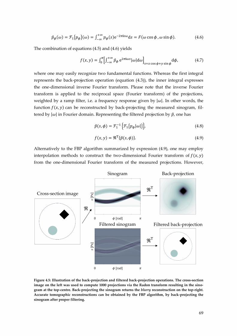
69

��𝜙(𝜔) = ℱ1{𝑝𝜙}(𝜔) = ∫ 𝑝𝜙(𝑠)e−2𝜋𝐢𝑠𝜔d𝑠

+∞

−∞= 𝐹(𝜔 cos𝜙 ,𝜔 sin𝜙). (4.6)

The combination of equations (4.5) and (4.6) yields

𝑓(𝑥, 𝑦) = ∫ [∫ ��𝜙+∞

−∞e2𝜋𝐢𝜔𝑠|𝜔|d𝜔]

𝑠=𝑥 cos𝜙+𝑦 sin𝜙d𝜙

𝜋

0, (4.7)

where one may easily recognize two fundamental functions. Whereas the first integral

represents the back-projection operation (equation (4.3)), the inner integral expresses

the one-dimensional inverse Fourier transform. Please note that the inverse Fourier

transform is applied to the reciprocal space (Fourier transform) of the projections,

weighted by a ramp filter, i.e. a frequency response given by |𝜔|. In other words, the

function 𝑓(𝑥, 𝑦) can be reconstructed by back-projecting the measured sinogram, fil-

tered by |𝜔| in Fourier domain. Representing the filtered projection by ��, one has

��(𝑠, 𝜙) = ℱ1−1 {ℱ1{𝑝𝜙|𝜔|}}, (4.8)

𝑓(𝑥, 𝑦) = ℜT{��(𝑠, 𝜙)}. (4.9)

Alternatively to the FBP algorithm summarized by expression (4.9), one may employ

interpolation methods to construct the two-dimensional Fourier transform of 𝑓(𝑥, 𝑦)

from the one-dimensional Fourier transform of the measured projections. However,

Sinogram

Filtered sinogram

Back-projection

Filtered back-projection

Cross-section image

Figure 4.5: Illustration of the back-projection and filtered back-projection operations. The cross-section

image on the left was used to compute 1000 projections via the Radon transform resulting in the sino-

gram at the top-centre. Back-projecting the sinogram returns the blurry reconstruction on the top-right.

Accurate tomographic reconstructions can be obtained by the FBP algorithm, by back-projecting the

sinogram after proper filtering.

70

such interpolation must account for the change between polar to Cartesian coordinates,

which may become an additional challenge in the Fourier domain even with advanced

methods such as cubic or spline interpolation. Examples of a sinogram, filtered sino-

gram and tomographic reconstruction are presented in Figure 4.5.

Analytical methods for tomographic reconstruction have some advantages when com-

pared to iterative methods. The FBP algorithm, for example, is based on Fourier trans-

forms (implemented with the FFT algorithm [85], [91]) and a single back-projection

which makes it conveniently fast. Besides, there are only few parameters one needs to

adjust, its derivation is based on an analytical inversion formula and the reconstruction

behaviour is well understood.

On the other hand, besides being limited to parallel beam geometry, the FBP algorithm

relies on projections measured along the full angular range [0, 𝜋[ with significant high

angular resolution. The minimum number of projections necessary for a faithful (ab-

sence of artefacts) tomographic reconstruction is traditionally given by the Crowther

criterion [92] in terms of the specimen’s size and expected spatial resolution. Instead,

the same sampling condition can be easily derived from the Nyquist sampling theorem

assuming that all projections are evenly distributed over the full angular range [0, 𝜋[.

Having in mind the Fourier slice theorem, it is natural to choose a minimum number of

projections 𝑚 so that the Fourier transform of 𝑓(𝑥, 𝑦) can be defined in all its pixels.

Considering the angular spacing between projections Δ𝜙 as illustrated in Figure 4.6b,

(a) (b) (c)

Figure 4.6: Angular sampling requirements for tomographic reconstruction, and different filtering

functions for FBP. (a) Illustration of 𝑭(𝝎𝐜𝐨𝐬𝝓 ,𝝎𝐬𝐢𝐧𝝓) in polar coordinates, as expressed by the Fouri-

er slice theorem. The FFT algorithm samples in a regular Cartesian grid and thus 𝑭(𝝎𝐜𝐨𝐬𝝓 ,𝝎𝐬𝐢𝐧𝝓)

must be interpolated onto a Cartesian grid as shown in (b). To prevent aliasing artefacts, all pixels in 𝑭

must be assigned, and thus the angular distance (arc length) between two adjacent pixels must be

smaller than 𝚫𝝓𝑵

𝟐 pixels. This observation is valid, assuming that the Fourier transform preserves the

same number of pixels and that the total number of projections cover 𝝅 radians, 𝒎 × 𝚫𝝓 = 𝝅. (c) Exam-

ples of different filtering functions for the FBP algorithm, and their representation in Fourier space.

71

then

𝑚 ≥𝜋𝑁

2 . (4.10)

Moreover, in analytical reconstruction methods only a modest amount of noise in the

acquired data is tolerated and a priori knowledge about the sample system, such as

non-negativity for example, cannot be exploited during reconstruction. The ramp filter

|𝜔| in the inversion formula (4.7) acts as a high-pass filter, which may be problematic

in the presence of noise, amplifying its contribution in the reconstructed image. In or-

der to handle noisy data, the FBP algorithm is often modified by including an addi-

tional (low-pass) filter such as a Hamming, Hann, Shepp-Logan or cosine filter [93], as

illustrated in Figure 4.6c.

Iterative tomographic reconstruction

Iterative or algebraic methods for tomographic reconstruction do not rely on analytical

inversion formulas as the FBP algorithm. Instead, an approximate solution of the

tomographic cross-section is obtained by solving the inverse problem associated with a

discretized description of the tomography forward model, given by the linear system of

equations:

𝐀𝒙 = 𝒃. (4.11)

Here, in (4.11), 𝐀 ∈ ℝ𝑀×𝑁 is the system matrix that may be interpreted as a discrete Ra-

don transform operator, 𝒙 ∈ ℝ𝑁 is the vector form of the cross-section image, and

𝒃 ∈ ℝ𝑀 the vector form of the sinogram‡‡‡. The tomographic reconstruction procedure

boils down to finding a solution 𝒙∗ for the system of equations (4.11) given a set of

measured projections 𝒃 = 𝒃meas. The problem of solving (4.11) for 𝒙 given a certain 𝒃,

belongs to the mathematical family of inverse problems [80], that in turn belongs to the

class of ill-posed problems whenever they violate at least one of Hadamard’s conditions:

The solution exists,

the solution must be unique,

and the solution depends continuously on the data, i.e. it is stable and a small

change in the data translates only into a small change in the solution.

The first two Hadamard’s requirements for well-posedness of (4.11) fail whenever 𝐀 is

not square, i.e. the problem is either under- or overdetermined. Furthermore, even in

cases where 𝐀 is invertible (the solution exists and is unique), the stability condition

‡‡‡ For notation simplicity, in this chapter 𝑁 and 𝑀 correspond to the size (in Pixels) of the vec-

tor forms of 𝒙 and 𝒃, while in the previous chapters 𝑁 was used to denote the lateral size of an

image.

72

may not hold due to the presence of noise in the measured data 𝒃meas. Consequently,

the naïve solution 𝒙∗ = 𝐀−1𝒃meas is often dominated by noise and does not provide any

useful information. For these reasons, ill-posed inverse problems are often solved by

introducing an additional regularity to the problem so that a unique and stable solu-

tion can be found. One way to deal with an inconsistent linear system of the type

𝐀𝒙 = 𝒃meas is to replace it by a least-squares minimization problem

𝒙∗ = argmin𝒙

1

2‖𝒃meas −𝐀𝒙‖2

2. (4.12)

Furthermore, different cost-functions can be used, based on different norms (for exam-

ple L-1 norm) or by introducing particular regularization terms, as it has been men-

tioned in Chapter 3 for the XRF probe deconvolution problem. Moreover, different

iterative methods can be employed to solve (4.12) and thus there are almost an infinite

number of possible algorithms that one may derive for tomographic reconstructions of

discrete datasets. For historical reasons, I present in this chapter two of the main classes

of iterative methods commonly used for tomographic reconstructions: the algebraic

reconstruction techniques (ART) and the simultaneous iterative reconstruction tech-

niques (SIRT).

The most well-known and common method of the ART class is perhaps the Kaczmarz

method [94] for solving linear systems of equations, introduced to the CT community

by Gordon et al. in 1970 [95]. Iterative methods of the this class are categorized as row-

action methods, since they treat the equations one at a time during the iterative recon-

struction [95], [96]. For this reason, ART methods are said to be fully sequential. The

Kaczmarz algorithm updates 𝒙 at each iteration 𝑙, from an initial solution guess 𝒙[0]

with the update step

𝒙𝑖[𝑙+1] = 𝒙𝑖

[𝑙] + 𝛼[𝑙+1]𝒃𝑖meas−𝑎𝑖

T𝒙𝑖[𝑙]

‖𝑎𝑖‖22 𝑎𝑖 , 𝑙 = 1,2, … 𝑖 = 1,2,…𝑁, (4.13)

where 𝑎𝑖T represents the 𝑖th row of the system matrix 𝐀, and 𝛼 is a relaxation parameter

in the range ]0,2[. If the system of equations (4.11) is consistent, i.e. there is at least one

solution that verifies all the equations, then the Kaczmarz iteration method converges

to a solution 𝒙∗ that minimizes the L-2 norm in (4.12), provided that the initial solution

guess 𝒙[0] is the zero vector or belongs to the column space of 𝐀 [97].

Reconstruction methods of the SIRT class are distinguished from ART in the sense that

all elements of 𝒙 are updated simultaneously at each iteration step. In this case, the

solution for 𝒙 is updated at each iteration according to the formula

𝒙[𝑙+1] = 𝒙[𝑙] + 𝐂𝐀T𝐑(𝒃meas − 𝐀𝒙[𝑙]), 𝑙 = 1,2,… (4.14)

73

where 𝐂 and 𝐑 are symmetric positive matrices, that may be chosen differently to ob-

tain different regularized solutions. In (4.14) 𝐀T represents the back-transform opera-

tor. The cost-function of SIRT methods is also different from ART, as one minimizes a

weighted norm of the residual vector instead of the L-2 norm as defined in (4.12). This

way, for SIRT reconstruction algorithms:

𝒙∗ = argmin𝒙

1

2‖𝒃meas − 𝐀𝒙‖𝐑

2 , (4.15)

where ‖∙‖𝐑 denotes the weighted norm of a vector so that ‖𝒙‖𝐑2 = 𝒙T𝐑𝒙. In the classical

SIRT algorithm [96], [98], 𝐂 and 𝐑 are diagonal matrices containing the inverse sum of

the columns and rows of the system matrix so that 𝐂𝑗,𝑗 = 1 ∑ 𝐀𝑖,𝑗𝑖⁄ , and 𝐑𝑖,𝑖 = 1 ∑ 𝐀𝑖,𝑗𝑗⁄ .

Such matrices aim to compensate for the number of rays that hit each pixel of the im-

age and the number of pixels that are hit by each ray. If 𝐂 and 𝐑 are chosen as the iden-

tity matrix, then the update formula in (4.14) reduces to the Landweber iteration

scheme as in Chapter 3. Other variants include the Cimmino’s method, component

averaging (CAV) and diagonally relaxed orthogonal projection (DROP).

The main advantage of iterative methods compared to analytical reconstruction tech-

niques include their capability of returning faithful tomographic reconstructions in the

presence of noise or incomplete projection data. Besides, iterative methods allow the

introduction of prior information about the sample, such as non-negativity, and differ-

ent regularization strategies that may be helpful in mitigating reconstruction artefacts

and to decrease noise effects while preserving sharp edges in the image. Moreover,

dead pixels or phase residues can be excluded from the reconstruction process that

otherwise would introduce undesired artefacts. On the other hand, the major draw-

back of iterative methods is associated to their higher computation time sas each itera-

Phase-residue

Wrapped sinogram Sinogram derivative Derivative FBP

Figure 2: Tomographic reconstruction of a sinogram with phase wrapping by the modified filtered

back-projection algorithm proposed by Guizar et al. [99]. For demonstration purposes a phase-residue

was simulated by setting one pixel of the sinogram to 0 that after tomographic reconstruction translates

into a streak artefact as seen in the image on the right.

74

tion requires both a forward- and back-projection operation.

The application of analytical or algebraic reconstruction methods to X-ray projections is

straightforward as long as the measured data can be described by the linear system of

equations in (4.11). In the specific case of phase-contrast projections, provided by CDI

techniques, equation (4.11) breaks in pixels with phase-wrapping, and thus an addi-

tional phase unwrapping operation is required as already mentioned in Chapter 3. Al-

ternatively to phase unwrapping before tomographic reconstruction, a modified ver-

sion of the FBP algorithm has been devised by Guizar et al. [99] that makes use of the

sinogram derivative insensitive to phase-wrapping. The successful implementation of

this method requires that the phase gradients are not wrapped, or in other words, that

the difference in phase between two adjacent pixels in a projection is smaller than 𝜋.

However, the presence of phase-residues impedes a proper evaluation of the sinogram

gradient and consequently propagate as artefacts in the reconstructed tomogram. On

the other hand, iterative reconstruction methods have the ability to mask out, or to ex-

clude, faulty pixels, such as phase-residues, but do not necessarily take into account the

presence of phase-wrapping in the projection data. To deal with phase-wrapped pro-

jections we proposed that iterative reconstruction methods can be modified by intro-

ducing a wrapping operator in the residual vector before the solution update step [9]. In

our studies the wrapping operator 𝑄(𝑓) was implemented as

𝑄(𝑓) = arg[e𝐢𝑓]. (4.16)

Despite being a non-linear operator, we have empirically observed that our modified

version of the SIRT algorithm equipped with the wrapping operator in (4.16) and the

non-negativity constraint was able to retrieve accurate tomographic reconstructions

from wrapped phase-contrast sinograms. Although no general proof of convergence

has been so far derived, we have seen that our method requires that the projections are

only moderately wrapped, and that the reconstruction procedure is dominated by the

non-wrapped areas of the sinogram. An example of a tomographic reconstruction from

a wrapped sinogram is presented in Figure 4.7 using the derivative FBP algorithm, and

Figure 4.8 using the proposed phase-SIRT algorithm.

Tomographic alignment of high-resolution phase-contrast projections

So far, the methods described for tomographic reconstruction assume a precise

knowledge of the relative spatial orientation between projections, and location of the

tomographic rotation axis. In macro- or micro-CT applications this condition is easily

achieved using highly accurate and stable rotation stages. However, nano-tomographic

techniques based on high-resolution projection imaging methods, pose an additional

challenge as the positioning precision is limited by mechanical stabilities and sample

75

drifts caused by thermal effects [9], [100], [101]. For this reason, high-resolution elec-

tron tomography and X-ray nano-tomography rely on numerical registration (align-

ment) of projection images preceding tomographic reconstruction. There is a large va-

riety of tomographic alignment algorithms already described in the literature [102]–

[107] that make use of fiducial markers introduced in the sample, such as gold nano-

particles, or exploit other intrinsic properties between projections, such as cross-

correlation or centre-of-mass alignment methods. However, most of these methods are

user-dependent, relying on manual interaction and visual inspection that may impede

efficient data processing, especially given the ever increasing data sizes and acquisition

rates provided by synchrotron facilities. During my PhD studies we have introduced

an automated tomographic alignment algorithm that we showed to be able to estimate

and correct for translational and angular deviations of the expected sample positions.

Our proposed method has demonstrated promising results, in terms of three-

dimensional resolution enhancement, with simulated and real datasets. More details

about this work can be found in the Appendix under Automated angular and transla-

tional tomographic alignment and application to phase-contrast imaging or equiva-

lently in [9] and references therein.

Figure 4.8: Tomographic reconstruction of a wrapped sinogram (from Figure 4.7) at different iterations

using the classical SIRT, and phase-SIRT algorithms. Both reconstructions were done without non-

negativity constraint and by masking out (excluding) the pixel associated with a phase-residue. The

colour scale in each image was set from the minimum to maximum value of the reconstructed slice. The

introduction of the wrapping operator in the residual vector allowed the phase-SIRT algorithm to re-

turn accurate reconstructions in the presence of phase-wrapping, and the streak artefact is avoided by

excluding the phase-residue from the reconstruction procedure.

76

Combined three-dimensional phase retrieval and tomographic recon-

struction of scanning coherent diffraction imaging techniques

To date, the application of scanning CDI techniques to three-dimensions involves two-

dimensional ptychography reconstructions of the acquired projections precedent to

tomographic alignment and reconstruction. Motivated by the dose fractionation theo-

rem and resolution limitations due to radiation damage, as referred in Chapter 3, we

have extended scanning coherent diffraction imaging reconstructions to three-

dimensions. As both ptychography and tomographic reconstructions can be formulat-

ed as discrete inverse problems, we have tested the possibility of combining both re-

construction processes in a single non-linear optimization algorithm. To avoid an un-

necessary repetition of the description of our method I refer to the published work in

Annex or under the reference [45].

77

5. Multimodal techniques for the

characterization of solar cells “The role of the infinitely small in nature is infinitely great”.

Louis Pasteur

This chapter is devoted to reporting our experimental results from X-ray measure-

ments combining three different, but complementary, scanning techniques, namely X-

ray ptychography, XRF, and XBIC for the characterization of third-generation

Cu2ZnSnS4 (CZTS) kesterite solar cells.

As mentioned in Chapter 1, solar energy has a great potential to fulfil our energy needs

in the future given that we have the technology available to harvest it with reasonable

efficiency. The main advantage of thin film photovoltaics arises from the direct band

gap of the materials that constitute the active layer, which allows the use of a smaller

amount of materials, when compared to crystalline silicon solar cells. Consequently,

thin film solar cells can be fabricated on flexible substrates, opening a window for nov-

el technological applications, at the same time yielding lower production costs and

energy payback time. From the family of thin film photovoltaics, kesterite solar cells

based on the quaternary inorganic semiconductor Cu2ZnSnS4, distinguishes itself from

CdTe and CIGS (CuInxGa(1-x)Se2) technologies, by avoiding the use of scarce elements

such as In and Te, and highly toxic materials such as Cd, while still providing high

absorption coefficients (> 104 cm−1) and an ideal band gap (~1.45 eV) for visible light

absorption.

One of the major challenges in the development of high efficiency CZTS solar cells is

associated with its complex stoichiometry that promotes the formation of secondary

phases during its synthesis and annealing process [108]. These, from which ZnS, SnS2

or Cu2S are examples, are detrimental for solar cell operation, reducing its overall con-

version efficiency, and therefore should be avoided or controlled during manufactur-

ing. To investigate the local performance and relationship between chemical composi-

tion, charge collection efficiency and grain boundaries in a fully functional solar cell,

we suggest the complementary use of X-ray ptychography, XRF and XBIC techniques.

XBIC has already been applied to first-generation [109] and recently to second-

generation solar cells in combination with X-ray fluorescence measurements [52], from

which a correlation between the local chemical composition and device charge collec-

tion efficiency was derived. However, the same study has not been applied to kesterite

78

devices so far, to our knowledge, neither in combination with X-ray ptychography for

the imaging of fine structures or grain boundaries.

Sample preparation

The CZTS solar cell investigated in this experiment, with a demonstrated conversion

efficiency of 5.2%, was already characterized and published in the literature under the

reference [110], where a more detailed description about the device and its preparation

method can be found. The full device consists of a layered structure as shown in Figure

5.1. A Mo bilayer, serving as bottom electrode, was first deposited onto a soda lime

glass substrate by DC magnetron sputtering at 10 W/cm2 power density. On the bottom

electrode, kesterite precursors (Cu, Sn and Zn) were deposited by pulsed laser deposi-

tion (PLD) [111] under high vacuum (< 5 × 10−6 mbar), with a KrF excimer laser with

a wavelength of 248 nm, a fluence of 0.6 J/cm2 and a spot size of 4 mm2. In order to

form Cu2ZnSnS4, the metallic precursors must undergo an annealing step. In this case,

this was performed at 560°C in a rapid thermal processor in the presence of S and SnS

powder. A thin buffer layer of CdS was applied by chemical bath deposition, followed

by a ZnO window layer by RF magnetron sputtering. Finally, a layer of indium doped

tin oxide (ITO) serving as top electrode was applied by sputtering followed by evapo-

ration of a thin layer of MgF that acts as anti-reflective coating of the solar cell. From

the fully functional CZTS device, two different samples were prepared for our experi-

ment:

A Top-view sample was prepared by removing most of the soda lime glass sub-

strate by mechanical polishing, so that the sample is sufficiently thin to be im-

aged by ptychography. This sample was designed for combined ptychography

and XRF measurements in order to visualize the interface between different

grains, and to identify possible secondary chemical phases over a significant

(b)

-

+

(a)

Figure 5.1: (a) Schematics of the lamella sample and devised electrical contacts. (b) cross-section SEM

image of the different layers composing the solar cell (SEM image provided courtesy of Dr. Andrea

Crovetto).

79

large area.

A cross-section sample intended for Ptychography, XRF, and XBIC measure-

ments, consisting of a lamella of ca. 1 µm thickness was prepared by focused

ion beam (FIB) etching and is illustrated in Figure 5.1.

Experiment description

The ptychography, XRF and XBIC measurements were carried out at the hard X-ray

nano-probe beamline P06 at PETRA III at the German Electron Synchrotron (Deutsches

Elektronen-Synchrotron, DESY). In order to highlight the main constituents of the solar

cell active layer (Cu, Zn, Sn and S) and monitor the possible Ga deposition from the FIB

etching an X-ray beam energy of 10.4 keV was used with an average focus size of 60

nm (FWHM).

The samples were placed on a piezo stage, which allows both rotation and translations,

and is controlled by an interferometric positioning system composed by three different

laser sources. In order to reduce self-absorption effects, the samples were positioned

with an angle of 23° with respect to the fluorescence detector (Xspress 3) at a distance

of 2-3 cm. All measurements were done at the beam focus, with acquisition times vary-

ing from 10 ms to 100 ms, covering different areas of the samples with fields of view

ranging from 1 × 1 µm to 40 × 40 µm. The diffraction data were acquired at a distance

of 2.31 m with a PILATUS 1M detector. In practice, the effective detector area used for

ptychography reconstructions was 512 × 512 pixels which results in a ptychography

reconstructed pixel size of 7.2 nm. XBIC measurements were formed using the same

configuration as in Figure 3.13, with the aid of a lock-in amplifier with an amplification

gain of 1kV/mA and an optical chopper with a chopping frequency of 367 Hz. Aside

from the described samples, a standard reference sample RF11-200-S3236 by AXO was

measured using XRF, as it is required for proper quantification of the different ele-

ments mass concentration in the sample. The reference sample consisted of a 200 nm

ElasticScatteringW

Cu

Mo

Sr

W

Ar

K

Ca

La

Fe

Ni

Pb

Si

ElementNominal mass

fraction(ng/mm2)

Measured mass fraction

(ng/mm2)

Relative difference

(%)

Pb 77.8±3.7 40.29 48

La 117.0±10.9 108.9 7

Pd 27.7±2.9 27.07 3

Mo 8.3±0.1 25.38 206

Cu 22.1±1.9 22.14 0.2

Fe 39.6±4.4 38.26 0

Ca 166.1±7.2 155 7

Figure 5.2: On the left: XRF spectra and elemental fitting of the standard RF11-200-S3236. On the right:

expected and measured mass fractions for the elements in the standard sample.

80

thick SiN2 substrate membrane where 7 elements (Pb, La, Pd, Mo, Cu, Fe and Ca) were

deposited in extremely thin layers (ca. 1-3 atomic layers). The mass fractions of these

elements are in the range of ng/mm2, as shown in the table in Figure 5.2.

Technical challenges

During data acquisition we faced different challenges that prevented us from success-

fully applying the three proposed scanning techniques to the cross-section sample. The

electrical contacts prepared before the experiment turned out to be faulty during data

acquisition. Furthermore the optical chopper was found to be misaligned with the in-

coming beam at the very end of the experiment. At the same time a significant drop in

the beam flux was observed that we attributed to a misalignment of an optic compo-

nent (order sorting aperture). To solve these problems we decided to remove the order

sorting aperture which modified the incoming beam parameters returned by the fun-

damental parameters calibration approach for XRF. To replace the lamella sample with

faulty contacts we chose to perform XBIC measurements on a macroscopic sample ex-

tracted from a different solar cell device that has not been so far characterized. This is

referred to as backup top-view sample in Figure 5.6. The electric contacts were connect-

ed before the experiment with the help of Dr. Michael Stuckelberger without whom

this experiment would not have been possible.

Data analysis

Ptychography reconstructions were obtained with 1000 iterations of the ePIE algo-

rithm. The XRF spectra were fitted using the software PyMca [112], developed at the

European Synchrotron Radiation Facility (ESRF). The elemental quantification fol-

CuZn

CuFe

Zn

Sn

In

K

Cd

ArCl

S

Mo

Sr

Figure 5.3: Example of XRF spectra and elemental fitting of a scan from the top-view sample.

81

lowed the fundamental parameters approach described in Chapter 3. For the top-view

sample a matrix correction was applied to account for self-absorption effects in the

sample layered structure. Besides the elements that constitute the sample, additional

elements were included in the data fitting procedure to account for the experimental

setup, namely Ar, W, Ni, Cl, Sr and K. Furthermore, the Be window of the flight tube,

the Si detector, and the air between the sample and the XRF detector were included as

attenuators. The spectrum background was approximated using the statistics-sensitive

non-linear iterative peak clipping (SNIP) algorithm. The fundamental parameters were

then estimated, taken into account the XRF detector active area (4 cm2) and the angles

between incoming beam, sample and XRF detector. This calibration resulted in an es-

timated flux of 1.39 × 108 photons/s, so that the measured concentrations of the majori-

ty of elements of the standard sample are in best agreement with their expected values.

The large deviations for Mo and Pb as shown in Figure 5.2 are justified by the low in-

tensity values at their corresponding emission lines which yields large errors during

data fitting.

For the top-view sample, when accounting for self-absorption effects by matrix correc-

tion, PyMca is not able to properly assign mass concentrations to a given element if this

is present in more than one of the layers. This is of special relevance for Zn, as it ap-

pears in both ZnO and CZTS layers. Instead, the computed mass-fractions correspond

to the values expected if all Zn was present in only one of the 2 layers. For this reason,

a correction factor was applied to the Zn mass fractions in the CZTS layer based on the

theoretical values (estimated from the thickness and density of ZnO and CZTS) of the

ratio between total Zn mass in the ZnO and CZTS respectively.

Results

All collected XRF maps exhibits a non-uniform distribution of the elements composing

the CZTS layer. For brevity only the Cu and Zn maps are here illustrated. Two exam-

ples of the Zn and Cu mass concentration maps are presented in Figure 5.4 and Figure

5.5 for the top-view and lamella sample respectively. Specifically, Figure 5.5 shows the

presence of a ZnS grain, one of the detrimental phases that is known to decrease the

overall solar cell device.

For the reasons already mentioned, XBIC measurements were performed in a wide

field of view (1 × 1 μm2) for which the Zn and Cu mass fractions could not be properly

determined. The XBIC map in Figure 5.6 is thus compared with the total recorded fluo-

rescence counts and the Zn fluorescence counts. At this scale, the XBIC and XRF maps

are well correlated in the active areas of the solar cell, whereas the absence of the XBIC

signal is explained by the lack of top layers that compose one of the electrodes.

82

Conclusions

CZTS solar cell active layers were investigated using XRF, ptychography and XBIC to

distinguish between different chemical phases and to correlate them locally with the

solar cell device efficiency. The acquired XRF maps show a heterogeneous distribution

of the elements composing the CZTS active layer, a factor that should be avoided to

Figure 5.4: Phase shift, reconstructed from ptychography data, Zn and Cu mass-fractions for a scan of

the top-view sample. The contrast provided by the ptychography phase reconstruction relates mostly

with the thickness variations of the specimen also indicating possible grain boundaries. So far, a clear

correlation between the ptychography phase, Zn and Cu XRF maps is still to be found and fully under-

stood.

Figure 5.5: Phase shift, reconstructed from ptychography data, Zn and Cu mass-fractions for a scan of

the lamella sample. The acquired XRF maps suggest the presence of a ZnS grain in the CZTS active

layer, which may be responsible for local shunts and a decrease of the device overall efficiency.

Figure 5.6: XBIC, total XRF and Zn XRF counts for the backup top-view sample.

83

minimize the formation of secondary phases during the annealing process. This indi-

cates that there is still room for improvement during the synthesis of the CZTS active

layer of third-generation solar cells.

The ptychography reconstructions of the lamella sample did not exhibit clear grain

boundaries that correlate with the presence of a ZnS grain. Nonetheless, its high-spatial

resolution allows for local determination of the different layer thicknesses that may be

used to refine the XRF matrix correction setup.

Since the chemical heterogeneities of the sample are mostly observed at the micrometre

scale, the acquired XBIC maps did not contain enough resolution to observe a correla-

tion between charge collection efficiency and the local chemical composition of the so-

lar cell. Nonetheless, a good contrast between the active areas of the device and those

without the top electrode was observed suggesting that XBIC can be directly applied

for the study of third-generation solar cells, given that a sufficiently high spatial resolu-

tion can be obtained.

84

Bibliography [1] B. P. Company, “BP Statistical Review of World Energy 2018,” 2018.

[2] G. Janssens-Maenhout et al., “Global Greenhouse Gases Emissions EDGAR

v4.3.2.” [Online]. Available:

http://edgar.jrc.ec.europa.eu/overview.php?v=432&SECURE=123. [Accessed: 20-Aug-

2008].

[3] G. Janssens-Maenhout et al., “EDGAR v4.3.2 Global Atlas of the three major

Greenhouse Gas Emissions for the period 1970-2012,” Earth Syst. Sci. Data Discuss., no.

August, pp. 1–55, 2017.

[4] Stocker and V. B. and P. M. M. (eds. . T.F., D. Qin, G.-K. Plattner, M. Tignor,

S.K. Allen, J. Boschung, A. Nauels, Y. Xia, “Summary for Policymakers. In: Climate

Change 2013: The Physical Science Basis. Contribution of Working Group I to the Fifth

Assessment Report of the Intergovernmental Panel on Climate Change,” CEUR

Workshop Proc., vol. 1542, pp. 33–36, 2015.

[5] R. Perez and M. Perez, “A Fundamental Look At Supply Side Energy Reserves

For The Planet,” Int. Energy Agency SHC Program. Sol. Updat., vol. 62, no. April 2009,

pp. 4–6, 2015.

[6] N. Espinosa, M. Hösel, D. Angmo, and F. C. Krebs, “Solar cells with one-day

energy payback for the factories of the future,” Energy Environ. Sci., vol. 5, no. 1, pp.

5117–5132, 2012.

[7] R. Søndergaard, M. Hösel, D. Angmo, T. T. Larsen-Olsen, and F. C. Krebs,

“Roll-to-roll fabrication of polymer solar cells,” Mater. Today, vol. 15, no. 1–2, pp. 36–49,

2012.

[8] S. Westenhoff, I. A. Howard, and R. H. Friend, “Probing the morphology and

energy landscape of blends of conjugated polymers with sub-10nm resolution,” Phys.

Rev. Lett., vol. 101, no. 1, pp. 1–4, 2008.

[9] T. Ramos, J. S. Jørgensen, and J. W. Andreasen, “Automated angular and

translational tomographic alignment and application to phase-contrast imaging,” J.

Opt. Soc. Am. A, vol. 34, no. 10, pp. 1830–1843, 2017.

[10] P. Pellat-Finet, “Fresnel diffraction and the fractional-order Fourier transform,”

Opt. Lett., vol. 19, no. 18, p. 1388, 1994.

[11] C. J. R. Sheppard, “Free-space diffraction and the fractional fourier transform,”

J. Mod. Opt., vol. 45, no. 10, pp. 2097–2103, 1998.

[12] D. Mas, C. Ferreira, and J. Garcia, “Fresnel diffraction calculation through the

fast fractional Fourier transform,” Proc. SPIE, vol. 3490, pp. 461–464, 1998.

85

[13] R. W. Gerchberg and W. O. Saxton, “A practical algorithm for the

determination of phase from image and diffraction plane pictures,” Optik (Stuttg)., vol.

35, no. 2, pp. 237–246, 1972.

[14] J. R. Fienup, “Reconstruction of an object from the modulus of its Fourier

transform,” Opt. Lett., vol. 3, no. 1, p. 27, 1978.

[15] D. Sayre, “Some implications of a theorem due to Shannon,” Acta Crystallogr.,

vol. 5, no. 6, pp. 843–843, 1952.

[16] J. M. Rodenburg, “Ptychography and related diffractive imaging methods,”

Adv. Imaging Electron Phys., vol. 150, no. 07, pp. 87–184, 2008.

[17] J. M. Rodenburg, “A simple model of holography and some enhanced

resolution methods in electron microscopy,” Ultramicroscopy, vol. 87, no. 3, pp. 105–121,

2001.

[18] A. V. Martin et al., “X-ray holography with a customizable reference,” Nat.

Commun., vol. 5, pp. 1–8, 2014.

[19] T. Warwick et al., “A scanning transmission x-ray microscope for materials

science spectromicroscopy at the advanced light source,” Rev. Sci. Instrum., vol. 69, no.

8, pp. 2964–2973, 1998.

[20] J. Lawrence et al., “Scanning transmission X-ray , laser scanning , and

transmission electron microscopy mapping of the exopolymeric matrix of microbial

biofilms,” Appl. Environ. Microbiol., vol. 69, no. 9, pp. 5543–5554, 2003.

[21] W. Hoppe, “Beugung im inhomogenen Primärstrahlwellenfeld. I. Prinzip einer

Phasenmessung von Elektronenbeungungsinterferenzen,” Acta Crystallogr. Sect. A, vol.

25, no. 4, pp. 495–501, 1969.

[22] W. Hoppe and G. Strube, “Beugung in inhomogenen Primärstrahlenwellenfeld.

II. Lichtoptische Analogieversuche zur Phasenmessung von Gitterinterferenzen,” Acta

Crystallogr. Sect. A, vol. 25, no. 4, pp. 502–507, 1969.

[23] W. Hoppe, “Beugung im inhomogenen Primärstrahlwellenfeld. III.

Amplituden‐ und Phasenbestimmung bei unperiodischen Objekten,” Acta Crystallogr.

Sect. A, vol. 25, no. 4, pp. 508–514, 1969.

[24] R. Hegerl and W. Hoppe, “Dynamische Theorie der Kristallstrukturanalyse

durch Elektronenbeugung im inhomogenen Primärstrahlwellenfeld,” Berichte der

Bunsengesellschaft für Phys. Chemie, vol. 74, no. 11, pp. 1148–1154, 1970.

[25] P. W. Hawkes, Advances in Imaging and Electron Physics, vol. 150. 2008.

[26] M. Dierolf et al., “Ptychographic coherent diffractive imaging of weakly

scattering specimens,” New J. Phys., vol. 12, 2010.

86

[27] P. Thibault, M. Dierolf, A. Menzel, O. Bunk, C. David, and F. Pfeiffer, “High-

resolution scanning x-ray diffraction microscopy.,” Science, vol. 321, no. 5887, pp. 379–

82, 2008.

[28] H. M. L. Faulkner and J. M. Rodenburg, “Error tolerance of an iterative phase

retrieval algorithm for moveable illumination microscopy,” Ultramicroscopy, vol. 103,

no. 2, pp. 153–164, 2005.

[29] J. R. Fienup, “Phase retrieval algorithms: a comparison,” Appl. Opt., vol. 21, no.

15, pp. 2758–2769, 1982.

[30] O. Bunk, M. Dierolf, S. Kynde, I. Johnson, O. Marti, and F. Pfeiffer, “Influence of

the overlap parameter on the convergence of the ptychographical iterative engine,”

Ultramicroscopy, vol. 108, no. 5, pp. 481–487, 2008.

[31] P. W. Hawkes, Advances in Imaging and Electron Physics. 2010.

[32] R. H. T. Bates and J. M. Rodenburg, “Sub-ångström transmission microscopy: A

fourier transform algorithm for microdiffraction plane intensity information,”

Ultramicroscopy, vol. 31, no. 3, pp. 303–307, 1989.

[33] H. N. Chapman, “Phase-retrieval X-ray microscopy by Wigner-distribution

deconvolution,” Ultramicroscopy, vol. 66, no. 3–4, pp. 153–172, 1996.

[34] H. M. L. Faulkner and J. M. Rodenburg, “Movable aperture lensless

transmission microscopy: A novel phase retrieval algorithm,” Phys. Rev. Lett., vol. 93,

no. 2, pp. 023903-1, 2004.

[35] J. M. Rodenburg and H. M. L. Faulkner, “A phase retrieval algorithm for

shifting illumination,” Appl. Phys. Lett., vol. 85, no. 20, pp. 4795–4797, 2004.

[36] M. J. Dierolf, “Ptychographic X-ray Microscopy and Tomography,” 2015.

[37] A. T. Walden, “Robust deconvolution by modified Wiener filtering,” Geophysics,

vol. 53, no. 2, pp. 186–191, 1988.

[38] A. M. Maiden and J. M. Rodenburg, “An improved ptychographical phase

retrieval algorithm for diffractive imaging,” Ultramicroscopy, vol. 109, no. 10, pp. 1256–

1262, 2009.

[39] V. Elser, I. Rankenburg, and P. Thibault, “Searching with iterated maps,” Proc.

Natl. Acad. Sci., vol. 104, no. 2, pp. 418–423, 2007.

[40] P. Thibault, M. Dierolf, O. Bunk, A. Menzel, and F. Pfeiffer, “Probe retrieval in

ptychographic coherent diffractive imaging,” Ultramicroscopy, vol. 109, no. 4, pp. 338–

343, 2009.

[41] B. Enders and P. Thibault, “Ptypy: Ptychography reconstruction for Python.”

2014.

87

[42] M. Guizar-Sicairos and J. R. Fienup, “Phase retrieval with transverse translation

diversity : a nonlinear optimization approach Abstract :,” Opt. Express, vol. 16, no. 10,

pp. 9954–9962, 2008.

[43] R. Hesse, D. R. Luke, S. Sabach, and M. K. Tam, “Proximal Heterogeneous

Block Input-Output Method and application to Blind Ptychographic Diffraction

Imaging,” vol. 8, no. 1, pp. 426–457, 2014.

[44] M. Odstrčil, A. Menzel, and M. Guizar-Sicairos, “Iterative least-squares solver

for generalized maximum-likelihood ptychography,” Opt. Express, vol. 26, no. 3, p.

3108, 2018.

[45] T. Ramos, B. E. Grønager, M. S. Andersen, and J. W. Andreasen, “Direct 3D

Tomographic Reconstruction and Phase-Retrieval of Far-Field Coherent Diffraction

Patterns,” Pre-print, 2018.

[46] G. Zheng, R. Horstmeyer, and C. Yang, “Wide-field, high-resolution Fourier

ptychographic microscopy,” Nat. Photonics, vol. 7, no. 9, pp. 739–745, 2013.

[47] J. Sun, C. Zuo, J. Zhang, Y. Fan, and Q. Chen, “High-speed Fourier

ptychographic microscopy based on programmable annular illuminations,” Sci. Rep.,

vol. 8, no. 1, pp. 1–12, 2018.

[48] J. Sun, C. Zuo, L. Zhang, and Q. Chen, “Resolution-enhanced Fourier

ptychographic microscopy based on high-numerical-aperture illuminations,” Sci. Rep.,

vol. 7, no. 1, pp. 1–11, 2017.

[49] J. Sherman, “The theoretical derivation of fluorescent X-ray intensities from

mixtures,” Spectrochim. Acta, vol. 7, pp. 283–306, 1955.

[50] N. Carulina, “Monte Carlo simulation of the X-ray fluorescence excited by

discrete energy photons in homogeneous samples including tertiary inter-element

effects,” X-ray Spectrom., vol. 4, pp. 138–148, 1975.

[51] H. Hieslmair, A. A. Istratov, R. Sachdeva, and E. R. Weber, “New synchrotron-

radiation based technique to study localized defects in silicon: ‘EBIC’ with X-ray

excitation,” in 10th Workshop on Crystalline Silicon Solar Cell Materials and Processes, 2000,

pp. 162–165.

[52] M. I. Bertoni, J. Maser, and V. Rose, “Grain engineering: How nanoscale

inhomogeneities can control charge collection in solar cells,” Nano Energy, vol. 32, no.

November 2016, pp. 488–493, 2017.

[53] M. Stuckelberger et al., “Latest developments in the x-ray based characterization

of thin-film solar cells,” 2015 IEEE 42nd Photovolt. Spec. Conf., pp. 1–6, 2015.

[54] B. Watts, D. Queen, A. L. D. Kilcoyne, T. Tyliszczak, F. Hellman, and H. Ade,

“Soft X-ray beam induced current technique,” J. Phys. Conf. Ser., vol. 186, no. 1, p.

012023, 2009.

88

[55] M. Stuckelberger et al., “Charge Collection in Hybrid Perovskite Solar Cells:

Relation to the Nanoscale Elemental Distribution,” IEEE J. Photovoltaics, vol. 7, no. 2,

pp. 590–597, 2017.

[56] M. Stuckelberger et al., “Engineering solar cells based on correlative X-ray

microscopy,” J. Mater. Res., vol. 32, no. 10, pp. 1825–1854, 2017.

[57] K. S. Shah, J. C. Lund, and F. Olschner, “Charge collection efficiency in a

semiconductor radiation detector with a non-constant electric field,” IEEE Trans. Nucl.

Sci., vol. 37, no. 2, pp. 183–186, 1990.

[58] T. Ramos, J. W. Andreasen, and J. S. Jørgensen, “AutoTomoAlign.” 2017.

[59] A. M. Maiden, M. J. Humphry, F. Zhang, and J. M. Rodenburg,

“Superresolution imaging via ptychography,” J. Opt. Soc. Am. A, vol. 28, no. 4, pp. 604–

612, 2011.

[60] E. Wolf, “New theory of partial coherence in the space–frequency domain Part

I: spectra and cross spectra of steady-state sources,” J. Opt. Soc. Am., vol. 72, no. 3, pp.

343–351, 1982.

[61] E. Wolf, “New theory of partial coherence in the space-frequency domain. Part

II: Steady-state fields and higher-order correlations,” J. Opt. Soc. Am. A, vol. 3, no. 1, pp.

76–85, 1985.

[62] L. W. Whitehead et al., “Diffractive imaging using partially coherent X rays,”

Phys. Rev. Lett., vol. 103, no. 24, pp. 1–4, 2009.

[63] B. Abbey et al., “Lensless imaging using broadband X-ray sources,” Nat.

Photonics, vol. 5, no. 7, pp. 420–424, 2011.

[64] P. Thibault and A. Menzel, “Reconstructing state mixtures from diffraction

measurements,” Nature, vol. 494, no. 7435, pp. 68–71, 2013.

[65] P. Li, D. J. Batey, T. B. Edo, A. D. Parsons, C. Rau, and J. M. Rodenburg,

“Multiple mode x-ray ptychography using a lens and a fixed diffuser optic,” J. Opt.

(United Kingdom), vol. 18, no. 5, pp. 1–8, 2016.

[66] M. R. Howells et al., “An assessment of the resolution limitation due to

radiation-damage in X-ray diffraction microscopy,” J. Electron Spectros. Relat.

Phenomena, vol. 170, no. 1–3, pp. 4–12, 2009.

[67] J. C. H. Spence, U. Weierstall, and M. Howells, “Coherence and sampling

requirements for diffractive imaging,” Ultramicroscopy, vol. 101, no. 2–4, pp. 149–152,

2004.

[68] H. A. Z. and C. L. W. Richard M. Goldstein, R. M. Goldstein, H. A. Zebker, and

C. L. Werner, “Satellite Radar Interferometry: Two-dimensional Phase Unwrapping,”

Radio Science, vol. 23, no. 4. pp. 713–720, 1988.

89

[69] V. V. Volkov and Y. Zhu, “Deterministic phase unwrapping in the presence of

noise.,” Opt. Lett., vol. 28, no. 22, pp. 2156–2158, 2003.

[70] A. Rose, “A unified approach to the performance of photographic film,

television pickup tubes, and the human eye,” J. Soc. Motion Pict. Eng., vol. 47, no. 4, pp.

273–294, 1946.

[71] R. Hegerl and W. Hoppe, “Influence of Electron Noise on Three-dimensional

Image Reconstruction,” Zeitschrift für Naturforsch. A, vol. 31, no. 12, 1976.

[72] B. F. McEwen, K. H. Downing, and R. M. Glaeser, “The relevance of dose-

fractionation in tomography of radiation-sensitive specimens,” Ultramicroscopy, vol. 60,

no. 3, pp. 357–373, 1995.

[73] W. Chao, B. D. Harteneck, J. A. Liddle, E. H. Anderson, and D. T. Attwood,

“Soft X-ray microscopy at a spatial resolution better than 15 nm,” Nature, vol. 435, no.

7046, pp. 1210–1213, 2005.

[74] J. Deng et al., “Opportunities and limitations for combined fly-scan

ptychography and fluorescence microscopy,” Proc. SPIE, vol. 9592, p. 95920U–1–

95920U–9, 2015.

[75] J. Deng et al., “Simultaneous cryo X-ray ptychographic and fluorescence

microscopy of green algae,” Proc. Natl. Acad. Sci. U. S. A., vol. 112, no. 8, pp. 2314–2319,

2015.

[76] J. N. Clark, X. Huang, R. J. Harder, and I. K. Robinson, “Continuous scanning

mode for ptychography,” Opt. Lett., vol. 39, no. 20, p. 6066, 2014.

[77] X. Huang et al., “Fly-scan ptychography,” Sci. Rep., vol. 5, p. 9074, 2015.

[78] P. M. Pelz, M. Guizar-Sicairos, P. Thibault, I. Johnson, M. Holler, and A.

Menzel, “On-the-fly scans for X-ray ptychography,” Appl. Phys. Lett., vol. 105, no. 25,

pp. 3–8, 2014.

[79] P. C. Hansen, J. G. Nagy, and D. P. O’Leary, Deblurring Images - matrices, spectra,

and filtering, 1st ed. Philadelphia: Society for Industrial and Applied Mathematics, 2006.

[80] P. C. Hansen, Discrete Inverse Problems, 1st ed. Philadelphia: Society for

Industrial and Applied Mathematics, 2010.

[81] M. R. Hestenes and E. Stiefel, “Methods of conjugate gradients for solving

linear systems,” J. Res. Nat. Bur. Stand., vol. 49, no. 6, pp. 409–436, 1952.

[82] L. Landweber, “An iteration formula for Fredholm integral equations of the

first kind,” Am. J. Math., vol. 73, no. 3, pp. 615–624, 1951.

[83] R. V. Mises and H. Pollaczek‐Geiringer, “Praktische Verfahren der

Gleichungsauflösung,” ZAMM ‐ J. Appl. Math. Mech. / Zeitschrift für Angew. Math. und

90

Mech., vol. 9, no. 2, pp. 152–164, 1929.

[84] G. Polak, E., Ribiere, “Note sur la convergence de méthodes de directions

conjuguées,” ESAIM Math. Model. Numer. Anal., vol. 3, pp. 35–43, 1969.

[85] M. Frigo and S. G. Johnson, “FFTW: An adaptive software architecture for the

FFT,” ICASSP, IEEE Int. Conf. Acoust. Speech Signal Process. - Proc., vol. 3, pp. 1381–1384,

1998.

[86] A. M. Cormack, “Representation of a function by its line integrals, with some

radiological applications. II,” J. Appl. Phys., vol. 35, no. 10, pp. 2908–2913, 1964.

[87] A. M. Cormack, “Reconstruction of densities from their projections, with

applications in radiological physics,” Phys. Med. Biol., vol. 18, no. 2, pp. 195–207, 1973.

[88] H. G. N., “Computerized transverse axial scanning(tomography):Part I

description of system,” Br. J. Radiol., vol. 46, no. 552, pp. 1016–1022, 1973.

[89] J. Radon, “Über die Bestimmung von Funktionen durch ihre Integralwerte

längs gewisser Mannigfaltigkeiten,” Berichte über die Verhandlungen der Königlich-

Sächsischen Akad. der Wissenschaften zu Leipzig, Math. Klasse, vol. 64, pp. 262–277, 1917.

[90] L. A. Feldkamp, L. C. Davis, and J. W. Kress, “Practical cone-beam algorithm,”

J. Opt. Soc. Am. A, vol. 1, no. 6, p. 612, 1984.

[91] J. W. Cooley and J. W. Tukey, “An Algorithm for the Machine Calculation of

Complex Fourier Series,” Math. Comput., vol. 19, no. 90, p. 297, 1965.

[92] R. A. Crowther, D. J. DeRosier, and A. Klug, “The Reconstruction of a Three-

Dimensional Structure from Projections and its Application to Electron Microscopy,”

Proc. R. Soc. A Math. Phys. Eng. Sci., vol. 317, no. 1530, pp. 319–340, 1970.

[93] T. M. Buzug, Computed tomography: From photon statistics to modern cone-beam CT.

2008.

[94] S. Kaczmarz, “Angenäherte Auflösung von Systemen linearer Gleichungen

(Approximate Solution for Systems of Linear Equations),” Bull. Int. l’Académie Pol. des

Sci. des Lettres. Cl. des Sci. Mathématiques Nat. Série A, Sci. Mathématiques, vol. 35, pp.

355–357, 1937.

[95] R. Gordon, R. Bender, and G. T. Herman, “Algebraic Reconstruction

Techniques ( ART ) for Three-dimensional Electron Microscopy and X-ray

Photography,” J. Theor. Biol., vol. 29, no. 3, pp. 471–476, 1970.

[96] A. C. Kak and M. Slaney, “Algebraic Reconstruction Algorithms,” in Principles

of Tomographic Imaging, New York, USA: IEEE Press, 1987, pp. 275–296.

[97] P. P. B. Eggermont, G. T. Herman, and A. Lent, “Iterative algorithms for large

partitioned linear systems, with applications to image reconstruction,” Linear Algebra

91

Appl., vol. 40, pp. 37–67, 1981.

[98] P. Gilbert, “Iterative methods for the three-dimensional reconstruction of an

object from projections,” J. Theor. Biol., vol. 36, no. 1, pp. 105–117, 1972.

[99] M. Guizar-Sicairos et al., “Phase tomography from x-ray coherent diffractive

imaging projections,” Opt. Express, vol. 19, no. 22, pp. 21345–21357, 2011.

[100] C. C. Wang, C. C. Chiang, B. Liang, G. C. Yin, Y. T. Weng, and L. C. Wang,

“Fast Projection Matching for X-ray Tomography,” Sci. Rep., vol. 7, no. 1, pp. 1–10,

2017.

[101] M. Guizar-Sicairos et al., “Phase tomography from x-ray coherent diffractive

imaging projections,” Opt. Express, vol. 19, no. 22, pp. 21345–21357, 2011.

[102] R. Guckenberger, “Determination of a common origin in the micrographs,”

Ultramicroscopy, vol. 9, pp. 167–174, 1982.

[103] D. J. Azevedo, Stephen G. Schneberk, J. P. Fitch, and H. E. Martz, “Calculation

of the rotational centers in computed tomography sinograms,” IEEE Trans. Nucl. Sci.,

vol. 31, no. 4, pp. 1525–1540, 1990.

[104] J. C. Fung, W. Liu, W. J. de Ruijter, H. Chen, and C. K. Abbey, “Toward fully

automated high-resolution electron tomography,” J. Struct. Biol., vol. 116, no. 1, pp.

181–189, 1996.

[105] T. Donath, F. Beckmann, and A. Schreyer, “Automated determination of the

center of rotation in tomography data.,” J. Opt. Soc. Am. A. Opt. Image Sci. Vis., vol. 23,

no. 5, pp. 1048–57, 2006.

[106] F. Bleichrodt and K. J. Batenburg, “Image Analysis: 18th Scandinavian

Conference, SCIA 2013, Espoo, Finland, June 17-20, 2013. Proceedings,” in Image

Analysis, J.-K. Kämäräinen and M. Koskela, Eds. Berlin, Heidelberg, 2013, pp. 489–500.

[107] D. S. Stephan, “High-Resolution 3D Ptychography,” no. September 2012, 2013.

[108] P. J. Dale, K. Hoenes, J. Scragg, and S. Siebentritt, “A review of the challenges

facing kesterite based thin film solar cells,” Conf. Rec. IEEE Photovolt. Spec. Conf., no.

June 2015, pp. 002080–002085, 2009.

[109] T. Buonassisi et al., “Applications of synchrotron radiation X-ray techniques on

the analysis of the behavior of transition metals in solar cells and single-crystalline

silicon with extended defects,” Phys. B Condens. Matter, vol. 340–342, pp. 1137–1141,

2003.

[110] A. Cazzaniga et al., “Ultra-thin Cu2ZnSnS4 solar cell by pulsed laser

deposition,” Sol. Energy Mater. Sol. Cells, vol. 166, no. January, pp. 91–99, 2017.

[111] M. Frumar, B. Frumarova, P. Nemec, T. Wagner, J. Jedelsky, and M. Hrdlicka,

92

“Thin chalcogenide films prepared by pulsed laser deposition - new amorphous

materials applicable in optoelectronics and chemical sensors,” J. Non. Cryst. Solids, vol.

352, no. 6–7, pp. 544–561, 2006.

[112] V. A. Solé, E. Papillon, M. Cotte, P. Walter, and J. Susini, “A multiplatform code

for the analysis of energy-dispersive X-ray fluorescence spectra,” Spectrochim. Acta -

Part B At. Spectrosc., vol. 62, no. 1, pp. 63–68, 2007.

[113] H. H. Bauschke, P. L. Combettes, and D. R. Luke, “Phase retrieval, error

reduction algorithm, and Fienup variants: a view from convex optimization,” J. Opt.

Soc. Am. A, vol. 19, no. 7, p. 1334, 2002.

[114] J. H. Hubbell, Bibliography and Current Status of K,L, and higher shells fluorescence

yields for computations of photon energy-absorption coefficients. National Bureau of

Standards, 1989.

[115] F. Salvat, J. Fernández-Varea, and J. Sempau, PENELOPE-2006: A code system for

Monte Carlo simulation of electron and photon transport, vol. 4, no. 6222. 2006.

93

Annexes

94

95

96

97

98

99

100

101

102

103

104

105

106

107

Direct 3D Tomographic Reconstruction and Phase-Retrieval of Far-Field Coherent Diffraction Patterns T. Ramos1, Bastian E. Grønager2, Martin Skovgaard Andersen3, J. W. Andreasen2,*

1Technical University of Denmark, Department of Energy Conversion and Storage, Roskilde, Denmark 2Technical University of Denmark, Department of Physics, Lyngby Denmark 3Technical University of Denmark, Department of Applied Mathematics and Computer Science, Lyngby, Denmark *Corresponding author: jewa@dtu.dk

Abstract We present an alternative numerical reconstruction algorithm for direct tomographic reconstruction of a sample’s refractive indices from the measured intensities of its far-field coherent diffraction patterns. We formulate the well-known phase-retrieval problem in ptychography in a tomographic framework which allows for simultaneous reconstruction of the illumination function and the sample’s refractive indices in three dimensions. Our iterative reconstruction algorithm is based on the Levenberg-Marquardt algorithm and we demonstrate the performance of our proposed method with simulated and real datasets.

Introduction

The performance and behaviour of numerous engineering materials and biological systems in different scientific fields is largely determined by their internal structure down to the micro and nanoscale. The ability to image such nanoscale structures is considered to be a crucial tool for their study and understanding in order to promote their further development and research. X-ray microscopy is a non-invasive technique well suited for imaging such systems due to its minimal sample preparation requirements, high spatial resolution, high degree of penetration (compared with electron microscopy) possibility for quantitative measurements and in situ or operando experimental setups. Of the different X-ray microscopy variants, coherent diffraction imaging (CDI) techniques do not rely on X-ray imaging optics such as lenses and their spatial resolution is consequently not limited by lens aberrations or numerical apertures and has the potential to reach atomic length scales comparable to the illumination wavelength. Moreover, by relying on the diffractive properties of coherent radiation, CDI techniques are able to image samples with sizes smaller than the X-ray detector pixel itself and return quantitative information of the sample’s complex refractive index which is inaccessible by conventional X-ray transmission methods.

Forward scattering X-ray ptychography, first demonstrated in 2007 [1], is a scanning variant of CDI that aims to relax the requirements for finite sample sizes defined within a compact support, and plane incoming wave front, allowing for increased fields-of-view and the additional reconstruction of the illumination function. In a CDI experiment the incoming beam, described by the probe function, interacts with the sample and is attenuated and phase shifted before being propagated into an X-ray photon counting detector that measures its intensity. Without an imaging lens, any phase information of the wave-field is lost, giving rise to the so called missing-phase problem.

Ptychography or CDI phase retrieval algorithms replace the purpose of an image forming lens by recovering the unknown phase numerically, using iterative algorithms mostly based on some type of optimization scheme. A few exceptions to these methods exist with closed-form solutions [2], [3] but their high sampling requirements make their application practically infeasible.

3D ptychography or ptycho-tomography extends the unique capabilities of CDI techniques to a higher spatial dimension, relying on tomographic reconstruction algorithms to assemble three-dimensional volumes representing the sample’s refractive indices, from which the absorption properties and electron density may be deduced. Here, 3D ptychography is to be understood as described and should not be mistaken for the multi-slice reconstruction approach described in [4]. The combination of both CDI and tomographic methods is not direct, involving intermediate data analysis steps mostly concerning phase-unwrapping, background data normalization and tomographic alignment operations. Several methods to address these issues have already been presented in the literature [5]–[9] and have so far been successfully applied in different fields of applications.

As X-ray ptycho-tomography expands into new scientific areas and in situ and operando studies, the need for faster acquisition times is becoming a decisive factor for the success of an experiment. Besides, new generation synchrotrons will deliver higher fluxes with a superior degree of coherence, and thus the spatial resolution of CDI techniques will most likely be limited by radiation damage suffered by the sample, rather than the coherence properties of the beam. According to the dose fractionation theorem, introduced by Hegerl and Hoppe [10], [11], the dose required to achieve a given statistical significance for each voxel of the three-dimensional tomogram is the same as required to measure a single projection of the same voxel with the same statistical significance. So far, ptychographic reconstruction algorithms rely on a significant overlap between illuminations in different scanning coordinates in order to constrain the domain of possible solutions and accurately recover the phase contrast image. A direct combination of ptychographic reconstruction methods with tomographic algorithms is thought to be able to relax this illumination overlap requirement by reducing its domain to a single 3D volume instead of a series of 2D projections (see Figure 1). Additionally, 2D ptychography images may contain non-negligible reconstruction errors that result in artefacts or resolution deterioration during tomographic reconstruction [12], [13]. Such uncertainties are expected to diminish in a direct ptycho-tomography reconstruction algorithm, because all measured data is implicitly forced to be consistent within a single three-dimensional volume.

Figure 1: Schematic representation of the overlap between consecutive illuminations in a 2D (left) and 3D (right) ptychography setup. In 2D ptychography, the illumination overlap (represented by the hatched area) is enforced at each tomographic angle by taking scanning step sizes smaller than the probe function width. In a three-dimensional setup, the overlap constraint is applied on illuminations from adjacent projection angles that overlap in the 3D volume that defines the tomographic reconstruction field-of-view.

Recently, Gürsoy [14] has shown that the probe overlap constraint can be significantly relaxed if a combined ptycho-tomography reconstruction approach is applied. In his work, Gürsoy extended the error-reduction algorithm of Fienup [15], [16] to a tomographic setting by intercalating this iterative method with one iteration of the SIRT algorithm [17] for tomographic reconstruction implemented with an additional total-variation (TV) regularization in order to preserve the edges of the object. Besides his proof-of-concept and encouraging results, the method proposed by Gürsoy implicitly relies on the combination of two different optimization strategies with different cost-functions (the error-reduction and the SIRT algorithm). We suggest that improved reconstruction results may be possible if this problem is expressed as a single optimization problem instead of two separate ones with different cost functions. Other independent and relevant works combining phase-retrieval and tomographic reconstruction were developed by Maretzke [18], [19] and by Kostenko [20] applied to full-field imaging methods such as in-line near-field holography with encouraging results demonstrated for real datasets.

In our work, we present a general description of a ptychography experiment and a direct ptycho-tomography reconstruction algorithm based on a single optimization cost-function with the potential to deal with datasets exhibiting moderate phase-wrapping. Our reconstruction strategy is based on a non-linear optimization algorithm that we show is able to accurately recover three-dimensional reconstructions of both the real and imaginary part of the sample’s complex refractive index, simultaneously.

This document is structured as follows: First, we describe the general forward model for a ptychography experiment. Afterwards, we present our reconstruction technique as a regularized optimization algorithm that solves a quadratic approximation of the Poisson log-likelihood function between the measured intensities and those resulting from our forward model. The behaviour of the proposed algorithm is demonstrated for simulated and real datasets.

At this stage, the proposed reconstruction method relies on a good estimation of the relative alignment parameters between the sample and the detector at each scanning coordinate. In the presence of misalignments, if a reasonable tomographic reconstruction guess is available from the proposed reconstruction method, additional alignment refinement algorithms such as those in [5], [7], [9], [21], [22] could be applied.

Methods

In a far-field coherent diffraction imaging measurement, the recorded intensity 𝐼𝚯 of the diffracted X-ray wavefront at the detector plane can be modelled, in the absence of noise, according to the Fraunhofer approximation:

𝐼𝚯 ≅ |ℱ{𝜓𝚯}|2 = |Ψ𝚯|2. (1)

Here, 𝚯 generalizes a set of relative orientation parameters between the incoming wavefront and the sample. These include spatial translations between the illumination and the sample, tomographic rotation angles and other possible angular tilts that may occur during data acquisition. For a monochromatic coherent illumination, the free-space propagation of the exit-wave 𝜓𝚯, after beam-sample interaction, can be modelled by a simple two-dimensional Fourier transform ℱ. Please note that this approximation is only valid for far-field measurements whereas in the near-field a Fresnel propagator should be used instead.

In our work, we assume that the incoming illumination wavefront, described by a complex-valued probe function, is constant during data acquisition and thus, also for notation simplicity, it will be represented by a unique symbol, 𝑃. In practice this assumption is not always entirely true and it has been shown that ptychography reconstructions can be improved by refinement algorithms [23] that take local probe variations into consideration. Under the ‘thin sample’ condition [24], the interaction between the incoming wavefront and the sample can be approximated by a simple multiplicative relation so that

𝜓𝚯 = 𝑃𝑂𝚯, (2)

where 𝑂 is the so-called object function and is related to the complex transmissivity of the sample up to a constant phase term. Other first-order phase terms may appear during ptychography reconstructions but are associated with uncertainties in the exact position of the centre of the diffraction patterns [8], [24]. Most of the already existing ptychography algorithms aim to recover both the probe 𝑃 and the object function 𝑂𝚯 in an alternating optimization approach, by iteratively refining the initial guesses of these functions using different, but analogous, strategies [24]–[28]. In turn, 𝑂 can also be defined as a function of the sample’s complex refractive index 𝑛 as

𝑂(𝑥, 𝑦) = exp [2𝜋𝐢

𝜆∫(𝑛(𝑥, 𝑦, 𝑧) − 1)d𝑧] , (3)

where 𝜆 represents the wavelength of the incoming X-ray beam, 𝐢 is the imaginary unit, 𝑥, 𝑦 and 𝑧 represent the spatial coordinates of the object expressed in a fixed coordinate system where 𝑧 is the direction of the incoming (and propagated) parallel X-ray beam, assumed to be perpendicular to the detector plane. For a given refractive index, 𝑛 = 1 − 𝛿 + 𝐢𝛽, the local electron density of the sample 𝜌𝑒 and linear absorption coefficient 𝜇 may be deduced according to

𝜌𝑒(𝑥, 𝑦, 𝑧) =2𝜋𝛿(𝑥,𝑦,𝑧)

𝑟0𝜆2 , (4)

𝜇(𝑥, 𝑦, 𝑧) =4𝜋𝛽(𝑥,𝑦,𝑧)

𝜆, (5)

where 𝑟0 = 2.82 ∙ 10−5 Å is the Thomson scattering length or classical electron radius.

Forward model

The description of our forward model follows naturally from the combination of (1), (2) and (3)

𝐼𝚯𝑓

= 𝐹(𝑛′) = |ℱ{𝑃 ∙ exp[𝐢𝑘ℛ𝚯(𝑛′)]}|2, (6)

where the wave number is defined as 𝑘 =2𝜋

𝜆 and ℛ𝚯 represents a linear operator that computes the line

integral in equation (3) expressed in terms of the relative sample-beam orientation parameters 𝚯. For notation simplicity we introduced 𝑛′ = 𝑛 − 1 = −𝛿 + 𝐢𝛽, that is the argument of our forward model and that we aim to resolve by our proposed method.

Reconstruction algorithm

As the phase information of the wavefront is lost in data acquisition, the inverse of our forward model 𝐹−1 cannot be defined uniquely. Also, the presence of noise in the measurements and small differences between the numerical model in equation (6) and the real physical phenomenon, make this inverse problem ill-posed.

The fundamental idea behind our reconstruction algorithm is analogous to those in traditional ptychography methods, meaning that it searches iteratively for a complex solution ��′, for the refractive indices of the sample, that minimize the differences between the experimentally measured intensities 𝐼𝚯

𝑚

and those resulting from the forward model in equation (6) 𝐼𝚯𝑓

. We choose as our object function the

quadratic approximation of the log-likelihood function [29] for the family of normal distributions 𝑁(𝜇𝑁 , 𝜎𝑁

2) with unknown mean 𝜇𝑁 and variance 𝜎𝑁2 defined as

𝑙(𝜇𝑁 , 𝜎𝑁2, 𝑥) = −

1

2𝜎𝑁2

∑ (𝑥𝑖 − 𝜇𝑁)2𝑖 , (7)

where 𝑥𝑖 denotes the intensity measurement/observation at the 𝑖 -th pixel. In an X-ray diffraction experiment, the measured intensities follow Poisson statistics, meaning that noise is uncorrelated between pixels and its variance for each pixel can be approximated by the mean measured intensity. Maximizing equation (7) is mathematically equivalent to minimizing the quadratic approximation of the negative log-likelihood, which in turn is expressed as the least-squares problem:

min𝑛′

𝑓(𝑛′) =1

2∑ (

𝐼𝚯𝑖

𝑓(𝑛′)−𝐼𝚯𝑖

𝑚

𝜎𝑖)

2

𝑖 . (8)

In our implementation the standard deviation in equation (8) is approximated by 𝜎 ≈ √𝐼𝚯𝑚 + 𝜖 in order to

decouple any dependence between the noise model and our forward model in (6). Also, the constant 𝜖 = 1 is used in order to avoid divisions by zero that may introduce numerical errors during reconstruction that are associated with pixels with zero measured intensities. Besides the ill-posed nature of this problem, the forward model (6) is also non-linear because of the squared modulus operator and the exponential function. This suggests that candidate solvers for equation (8) belong to the family of non-linear regularized least-squares minimization algorithms as is the case for the (non-linear, regularized) Gauss-Newton [30], Levenberg-Marquardt [31], [32] and Powell’s Dog Leg method, among others. In our work, the problem in equation (8) is solved with the Levenberg-Marquardt algorithm (LMA), also known as damped Gauss-

Newton method. Let us define a vector-valued function 𝑟(𝑛′) =𝐼𝚯

𝑒(𝑛′)−𝐼𝚯𝑚

√𝐼𝚯𝑚+𝜖

, also known as residual vector, so

that

1

2∑ (

𝐼𝚯𝑖

𝑓(𝑛′)−𝐼𝚯𝑖

𝑚

√𝐼𝚯𝑚+𝜖

)

2

𝑖 =1

2𝑟(𝑛′)∗𝑟(𝑛′). (9)

Here the superscript ‘∗’ represents the adjoint or conjugate transpose operator. The gradient and Hessian of the cost function 𝑓(𝑛′) are expressed as

∇𝑓(𝑛′) = 𝐽(𝑛′)∗𝑟(𝑛′), (10)

∇2𝑓(𝑛′) = 𝐽(𝑛′)∗𝐽(𝑛′) + 𝑄(𝑛′), (11)

where 𝐽(𝑛′) =𝜕𝑟

𝜕𝑛′ =1

√𝐼𝚯𝑚+𝜖

𝜕𝐼𝚯𝑓

(𝑛′)

𝜕𝑛′ is the Jacobian of 𝑟(𝑛′), and 𝑄(𝑛′) denotes higher order quadratic terms

of the Hessian that are often ignored for many large scale problems to improve computational efficiency. The cost function 𝑓(𝑛′) can be linearized around a current estimate of a minimizing point by means of a second-order Taylor expansion expressed as a function of the Jacobian and Hessian as

𝑓(𝑛′ + ∆𝑛′) ≈ 𝑓(𝑛′) + ∇𝑓(𝑛′)∆𝑛′ +1

2∆𝑛′∗

∇2𝑓(𝑛′)∆𝑛′. (12)

As most numerical minimization algorithms, the LMA adjusts an initial guess for 𝑛′ by taking an update step ℎ𝑛′ = ∆𝑛′ that minimizes the quadratic cost-function. This is done by differentiating (12) and computing its roots. This way, at the 𝑙-th iteration, we define:

ℎ𝑛′[𝑙]

= −(∇2𝑓(𝑛′[𝑙]) + 𝜆𝑙𝑚)−1

∇𝑓(𝑛′[𝑙]), (13)

𝑛′[𝑙+1] = 𝑛′[𝑙] + ℎ𝑛′[𝑙]

. (14)

In equation (13), 𝜆𝑙𝑚 is a damping factor, introduced by Levenberg [31] that regularizes the Hessian and is updated at each iteration. Considering the aforementioned first-order approximation of the Hessian, both ∇𝑓(𝑛′) and ∇2𝑓(𝑛′) require the definition of 𝐽(𝑛′) and its adjoint 𝐽(𝑛′)∗. As in the work by Maretzke [18],

[19] we express these functions implicitly, depending on the current reconstruction 𝑛′[𝑙]:

𝐽 (𝑛′[𝑙]) ℎ

𝑛′[𝑙]

=1

√𝐼𝚯𝑚+𝜖

ℜ [(ℱ{𝑃 ∙ exp[𝐢𝑘ℛ𝚯(𝑛′[𝑙])]})

ℱ {𝐢𝑘𝑃 ∙ exp [𝐢𝑘ℛ𝚯 (𝑛′[𝑙]

)] ℛ𝚯 (ℎ𝑛′[𝑙]

)}] =

1

√𝐼𝚯𝑚+𝜖

ℜ [(Ψ𝚯[𝑙]) ℱ {(𝐢𝑘𝜓𝚯

[𝑙])ℛ𝚯 (ℎ𝑛′[𝑙]

)}], (15)

𝐽 (𝑛′[𝑙])

∗ℎ𝑔

[𝑙]= ℛ𝚯

∗ [𝐢𝑘𝑃 ∙ exp[𝐢𝑘ℛ𝚯(𝑛′[𝑙])] ℱ−1 {

1

√𝐼𝚯𝑚+𝜖

(ℱ {𝑃 ∙ exp [𝐢𝑘ℛ𝚯 (𝑛′[𝑙])]}) ℜ [ℎ𝑔

[𝑙]]}] =

2ℛ𝚯∗ [(𝐢𝑘𝜓𝚯

[𝑙]) ℱ−1 {

Ψ𝚯[𝑙]ℜ[ℎ𝑔

[𝑙]]

√𝐼𝚯𝑚+𝜖

}]. (16)

In equations (15) and (16) the overbar denotes complex conjugation, ℜ is the real-part (self-adjoint) operator and ℛ𝚯

∗ generalizes the tomographic back-transform according to the fields-of-view and sampleorientation parameters described by 𝚯.

Probe Retrieval

In most CDI experiments, the probe function 𝑷 may not be known or available, but it can be retrieved by ptychography algorithms in an alternating optimization approach. In our work we follow the same method for reconstructing 𝒏′ in order to recover 𝑷, intercalating both optimization problems after each iteration of the proposed algorithm. The probe reconstruction problem is then formulated as

�� = argmin𝑃

1

2∑ (

𝐼𝚯𝑖

𝑓(𝑃)−𝐼𝚯𝑖

𝑚

𝜎𝑖)

2

𝑖 . (17)

Here, the Jacobian and Hessian approximations are expressed as functions of 𝐽𝑝(𝑃) and 𝐽𝑝(𝑃)∗, that in turn

are given by

𝐽𝑃(𝑃[𝑙])ℎ𝑃[𝑙]

=1

√𝐼𝚯𝑚+𝜖

ℜ [(Ψ𝚯[𝑙]) ℱ {𝑂𝚯

[𝑙]ℎ𝑃}], (18)

𝐽𝑃(𝑃[𝑙])∗ℎ𝑔

[𝑙]= 2𝑂𝚯

[𝑙] ℱ−1 {

Ψ𝚯[𝑙]ℜ[ℎ𝑔

[𝑙]]

√𝐼𝚯𝑚+𝜖

}. (19)

Discretization and Implementation

The linear operator ℛ𝚯 and its adjoint were implemented using the ASTRA toolbox [33] in order to exploit GPU resources for faster computations on large datasets. Besides, a full description of the relative positioning between incoming beam, sample and detector is allowed, enabling the reconstruction of datasets acquired with more complex scanning geometries. This flexible operator can also be used to correct for any known translational or angular motion that the sample may experience during measurements i.e. vibrations or wobbling of the rotation axis. The 2D Fourier transform ℱ and its adjoint/inverse were implemented using the FFTW library [34] and all multiplications in equations (6), (14) and (15) are to be understood element-wise. The developed algorithms were implemented and tested using MATLAB®2017a and Python2 on both Windows and Linux platforms and are publically available online under the DOI: 10.6084/m9.figshare.6608726.

Each iteration of the LMA, computes the solution update step in equation (13) by solving the least-squares problem:

(𝐽∗[𝑙]𝐽[𝑙] + 𝜆𝑙𝑚𝐈)ℎ𝑛′[𝑙]

= −𝐽∗[𝑙]𝑟[𝑙], (20)

using the Hestenes-Stiefel version of the conjugate gradient method (CGM)[35], [36]. In equation (20), 𝐈 is the identity matrix. In turn, the damping term of the LMA, 𝜆𝑙𝑚 is updated at each iteration using the strategy in [37].

The application of constraints in 𝑛′, after each solution update, is seen to be essential for accurate quantitative reconstruction of the refractive indices of the sample. These become particularly important in order to resolve datasets with wrapped phases in the object function (3). In our implementation, a non-

negativity constraint is applied to 𝑛′, after each iteration, limiting the domain of 𝛿 and 𝛽 to only non-negative numbers. Once a new solution for 𝑛′ is computed we write

𝑛′[𝑙]= −𝛿[𝑙] + 𝐢𝛽[𝑙] = min(−𝛿[𝑙], 0) + 𝐢 max(𝛽[𝑙], 0). (21)

The resulting reconstruction algorithm is summarized in the pseudocode Algorithm 1:

Algorithm 1: Tomographic Reconstruction of Far-Field Coherent Diffraction Patterns

1. Initialize 𝑛′, 𝜆𝑙𝑚

2. While 𝑙 < 𝑙𝑚𝑎𝑥 or not stop-criterion do:

Use forward model to compute

𝐹[𝑙] = 𝐹(𝑛′[𝑙])

Solve (12) using CGM (Hestenes-Stiefel):

(𝐽∗[𝑙]𝐽[𝑙] + 𝜆𝑙𝑚𝐈)ℎ𝑛′[𝑙]

= −𝐽∗[𝑙]𝐹[𝑙]

Update sample solution

𝑛′[𝑙+1] = 𝑛′[𝑙] + ℎ𝑛′[𝑙]

Enforce constraints to sample solution

Update 𝜆𝑙𝑚

Solve using CGM (Hestenes-Stiefel):

(𝐽𝑃∗[𝑙]

𝐽𝑃[𝑙] + 𝜆𝑙𝑚,𝑃𝐈) ℎ𝑃

[𝑙]= −𝐽𝑃

∗[𝑙]𝐹[𝑙]

Update probe solution

𝑃[𝑙+1] = 𝑃[𝑙] + ℎ𝑃[𝑙]

Enforce constraints to Probe solution

Update 𝜆𝑙𝑚,𝑃

End While

Simulation setup

A 3003-voxel discretized complex-valued phantom was used to generate 4000 diffraction patterns randomly distributed over 180 degrees around the rotation axis of the sample. These were computed using the forward model in equation (6) and afterwards rounded to integer numbers. Four different simulations were conducted in order to evaluate the robustness of our algorithm in the presence of noise and weakly-absorbing samples. In this context, weakly-absorbing samples are understood as those with 𝛽 ≪ 𝛿. The

simulated 𝛿 and 𝛽 values are in the range of 0 to 10−5 for two of the simulations, whereas for the weakly-absorbing samples the 𝛽 ranges from 0 to 10−7. The detector with 1002 pixels of 172 µm was placed at 5 m from the sample, which for a wavelength of 1 Å corresponds to a reconstructed voxel size of 29 nm. The probe function was generated using a Gaussian function, with a total integrated intensity of 107 photons and is illustrated in Figure 2. The generated 𝛿 and 𝛽 volumes are depicted in Figure 3 for the weakly-absorbing sample case. In this work the real and imaginary part of the simulated phantom were generated

Figure 2: Amplitude and phase of the complex-valued probe function used in our simulations.

independently with different structures. This was done in order to demonstrate a good reconstruction performance for cases where no explicit dependence between 𝛿 and 𝛽 may be expressed.

When imaging samples with high 𝛿 and/or large thicknesses, phase shifts of the object function (equation (3)) may be larger than 𝜋 resulting in wrapping of the phase. Current reconstruction strategies rely either on phase-unwrapping algorithms [38]–[40] of the phase-contrast projections prior to tomographic reconstruction, or alternative tomographic reconstruction algorithms such as those in [8], [9]. In order to

evaluate the robustness of our reconstruction method in the presence of phase-wrapping a simulated

sample with 𝛿 values in the range of [0 ~ 5 × 10−5] was used resulting in phase-wrapping of the object function as shown in Figure 5b.

All tomographic reconstructions presented in this document were obtained using 25 iterations of the CGM and 50 iterations of the LMA, except for the datasets with phase-wrapping where 100 iterations of the LMA were used instead.

Results and Discussion

The final reconstructions of simulated data, using our proposed reconstruction algorithm, are presented in Figure 4. Our results suggest that Poisson noise in the measurements decreases the reconstruction quality as is intuitively expected, and is responsible for artefacts during the initial reconstruction iterations. Such artefacts arise from erroneous contributions of the real part of the solution update ℎ𝑁 into its imaginary part or vice versa. We also found that reconstructing 𝛽 for weakly-absorbing samples is increasingly challenging as the results in Figure 4 illustrate. We believe that this effect can be explained by the difference in orders of magnitude between the 𝛿 and 𝛽 values of the sample. When such difference is large our reconstruction method is mostly dominated by updates of the 𝛿 volume that have a higher impact on

Figure 3: Complex-valued phantom used in our simulations. On the top: 3D isosurface and cross-section over cardinal planes for simulated 𝜹 object. On the bottom: Same for simulated 𝜷 volume.

the cost-function in equation (8). On the other hand, when the 𝛽 and 𝛿 are in the same order of magnitude, the reconstructed tomograms are in good agreement with both the real and imaginary parts of the sample’s refractive indices.

The full proof of convergence of our proposed method in the presence of large phase-shifts (> 𝜋) is not part of the scope of this publication. Nonetheless, our simulations indicate that by the use of appropriate constraints, such as the one in equation (21) and at the cost of additional iterations, accurate tomographic reconstructions can be achieved by the reconstruction algorithm as exhibited in Figure 5.

An example of application of the proposed algorithm to a real dataset is presented in Figure 6. The diffraction data was acquired at the cSAXS beamline from the Paul Scherrer Institut from a LiFePO4 powder sample inside a glass capillary tube. A total of 200 ptychography projection images were reconstructed by the difference map algorithm with maximum-likelihood probe positioning refinement [23], [27], [41] from 172 different scanning positions each. As our proposed reconstruction algorithm requires handling all

Figure 4: X-Y tomographic slices of the reconstructed refractive index for simulation data. The reconstructed 𝜹 volumes are represented at the top and the 𝜷 on the bottom. From left to right: low-absorption noise-free; low-absorption Poisson noise; high-absorption noise-free; high-absorption Poisson noise. The intensity scale in each image was properly normalized according

to the refractive index of the sample i.e. [𝟎~𝟏𝟎−𝟓] for all images except for the 𝜷 representations with low-absorption where

[𝟎~𝟏𝟎−𝟕] was used instead.

Figure 5: Comparison between tomographic reconstructions, by the proposed algorithm, from datasets with and without phase-wrapping of the object function. (a) and (b) illustrate the phase-shifts of the object function without and with phase-phase-wrapping respectively. (c) and (d) show X-Y slices from tomographic reconstructions exhibiting an accurate reconstruction of 𝜹 for the dataset containing wrapped phases (or large phase-shifts).

diffraction patterns at once, we saw ourselves limited by its high memory demands both in terms of RAM and GPU onboard memory. For this reason, we show the behaviour of our reconstruction method by using only a small fraction of the total acquired dataset. For the reconstruction in Figure 6c the diffraction patterns were cropped to their central 300 × 300 pixels and in Figure 6d to their central 400 × 400 pixels. Please note that this operation results in an increase of the reconstructed voxel size from 14.3 nm to 28.6 nm and 21.5 nm for Figure 6c and Figure 6d respectively, and consequently to a decrease in spatial resolution. Furthermore, the reconstruction in Figure 6d was obtained by using only 1/4th of the total diffraction patterns. Due to computational limitations, our reconstruction algorithm was run with only 20 iterations for both CGM and LMA algorithms, which in this case were sufficient to illustrate the main features of the sample inner structure. Improvements in reconstruction accuracy and resolution could be achieved, for example, by increasing the number of iterations taken in both CGM and LMA, and the amount or size of the diffraction data used. We expect that it will soon be possible to handle full data sets with the advent of memory architectures linked across several GPU’s.

(a)

(c)

(b)

(d)

Figure 6: Tomographic reconstructions of 𝜹 values obtained by different reconstruction approaches: (a) Filtered backprojection of 200 uniformly distributed projections. (b) Tomographic reconstruction with 1/4th of the dataset (50 projections). Because of the reduced number of projections the reconstruction was obtained by the SIRT algorithm with 200 iterations. (c) Tomographic reconstruction by the proposed algorithm with 20 iterations of the CGM and 15 iterations of the LMA algorithm. (d) Tomographic reconstruction by the proposed algorithm with 20 iterations of the CGM and 20 iterations of the LMA algorithm with 1/4th of the total diffraction patterns dataset. Reconstructed voxel sizes of 14.3 nm for for (a) and (b), 28.6 nm for (c) and 21.5 nm for (d). The greyscale varies linearly with the 𝜹 values from 0 (white) to 𝟏 ×

𝟏𝟎−𝟓 (black).

Conclusions and future work

In this work we have presented a numerical algorithm for direct tomographic reconstruction of the volumetric distribution of the refractive index of a sample from intensity measurements of far-field coherent diffraction patterns. This non-linear and ill-posed inverse problem is framed as a least-squares optimization problem, taking into account Poisson noise statistics in the measured intensities, which we solve by the Levenberg-Marquardt algorithm. Our simulation results show that accurate reconstruction of the sample’s refractive indices can be retrieved by the proposed method, which is of special interest for phase-contrast tomography experiments. Our studies also indicate that the convergence of this proposed reconstruction method is mostly dominated by the highest values of 𝑛′, making the reconstruction of the absorption properties of the sample increasingly challenging for the cases where 𝛽 ≪ 𝛿.

Future improvements to our proposed algorithm will include the implementation of other regularization methods, such as Tikhonov (for noise suppression) and total variation (for edge-enhancement) in our optimization problem. Additional constraints in both direct and/or reciprocal space may also benefit the convergence of the proposed reconstruction method by restricting/bounding the solution space of our problem. We are currently working on a multiscale reconstruction approach to decrease the total computational time by first reconstructing a low-resolution version of the object that is then taken as initial solution guess for the high-resolution reconstruction.

So far, all the presented tomographic reconstructions relied on the exact knowledge of the probe function and the sample spatial coordinates at each scanning position. The extension of the proposed method for probe retrieval is an ongoing endeavour.

References [1] J. M. Rodenburg, A. C. Hurst, A. G. Cullis, B. R. Dobson, F. Pfeiffer, O. Bunk, C. David, K. Jefimovs, and

I. Johnson, “Hard-X-ray lensless imaging of extended objects,” Phys. Rev. Lett., vol. 98, no. 3, pp. 1–4, 2007.

[2] J. M. Rodenburg and R. H. T. Bates, “The Theory of Super-Resolution Electron Microscopy Via Wigner-Distribution Deconvolution,” Philosophical Transactions of the Royal Society A: Mathematical, Physical and Engineering Sciences, vol. 339, no. 1655. pp. 521–553, 1992.

[3] H. N. Chapman, “Phase-retrieval X-ray microscopy by Wigner-distribution deconvolution,” Ultramicroscopy, vol. 66, no. 3–4, pp. 153–172, 1996.

[4] A. M. Maiden, M. J. Humphry, and J. M. Rodenburg, “Ptychographic transmission microscopy in three dimensions using a multi-slice approach,” J. Opt. Soc. Am. A, vol. 29, no. 8, p. 1606, 2012.

[5] P. Fomby and A. J. Cherlin, “Automatic alignment and reconstruction of images for soft X-ray tomography,” J. Struct. Biol., vol. 72, no. 2, pp. 181–204, 2011.

[6] S. Brandt, J. Heikkonen, and P. Engelhardt, “Automatic alignment of transmission electron microscope tilt series without fiducial markers.,” J. Struct. Biol., vol. 136, no. 3, pp. 201–213, 2001.

[7] F. Bleichrodt and K. J. Batenburg, “Automatic optimization of alignment parameters for tomography datasets,” in Image Analysis: 18th Scandinavian Conference, SCIA 2013, Espoo, Finland, June 17-20, 2013. Proceedings, Berlin, Heidelberg: Springer Berlin Heidelberg, 2013, pp. 489–500.

[8] M. Guizar-Sicairos, A. Diaz, M. Holler, M. S. Lucas, A. Menzel, R. a. Wepf, and O. Bunk, “Phase tomography from x-ray coherent diffractive imaging projections,” Opt. Express, vol. 19, no. 22, pp. 21345–21357, 2011.

[9] T. Ramos, J. S. Jørgensen, and J. W. Andreasen, “Automated angular and translational tomographic alignment and application to phase-contrast imaging,” J. Opt. Soc. Am. A, vol. 34, no. 10, pp. 1830–1843, 2017.

[10] R. Hegerl and W. Hoppe, “Influence of Electron Noise on Three-dimensional Image Reconstruction,” Zeitschrift für Naturforsch. A, vol. 31, no. 12, 1976.

[11] B. F. McEwen, K. H. Downing, and R. M. Glaeser, “The relevance of dose-fractionation in tomography of radiation-sensitive specimens,” Ultramicroscopy, vol. 60, no. 3, pp. 357–373, 1995.

[12] M. Odstrčil, A. Menzel, and M. Guizar-Sicairos, “Iterative least-squares solver for generalized maximum-likelihood ptychography,” Opt. Express, vol. 26, no. 3, p. 3108, 2018.

[13] M. Holler, A. Diaz, M. Guizar-Sicairos, P. Karvinen, E. Färm, E. Härkönen, M. Ritala, A. Menzel, J. Raabe, and O. Bunk, “X-ray ptychographic computed tomography at 16 nm isotropic 3D resolution,” Sci. Rep., vol. 4, p. 3857, 2014.

[14] D. Gürsoy, “Direct coupling of tomography and ptychography,” Opt. Lett., vol. 42, no. 16, pp. 3169–3172, 2017.

[15] J. R. Fienup, “Reconstruction of a complex-valued object from the modulus of its Fourier transform using a support constraint,” J. Opt. Soc. Am. A, vol. 4, no. 1, p. 118, 1987.

[16] J. R. Fienup, “Reconstruction of an object from the modulus of its Fourier transform,” Opt. Lett., vol. 3, no. 1, p. 27, 1978.

[17] P. Gilbert, “Iterative methods for the three-dimensional reconstruction of an object from projections,” J. Theor. Biol., vol. 36, no. 1, pp. 105–117, 1972.

[18] S. Maretzke, “Regularized Newton methods for simultaneous Radon inversion and phase retrieval in phase contrast tomography,” Georg-August-Universtität, 2015.

[19] S. Maretzke, M. Bartels, M. Krenkel, T. Salditt, and T. Hohage, “Regularized Newton Methods for X-ray Phase Contrast and General Imaging Problems,” Opt. Express, vol. 24, no. 6, pp. 6490–6506, 2016.

[20] A. Kostenko, K. J. Batenburg, A. King, S. E. Offerman, and L. J. van Vliet, “Total variation minimization approach in in-line x-ray phase-contrast tomography,” Opt. Express, vol. 21, no. 10, pp. 12185–12196, 2013.

[21] L. Houben and M. Bar Sadan, “Refinement procedure for the image alignment in high-resolution electron tomography,” Ultramicroscopy, vol. 111, no. 9–10, pp. 1512–1520, 2011.

[22] C. Yang, E. G. Ng, and P. A. Penczek, “Unified 3-D structure and projection orientation refinement using quasi-Newton algorithm,” J. Struct. Biol., vol. 149, no. 1, pp. 53–64, 2005.

[23] P. Thibault and M. Guizar-Sicairos, “Maximum-likelihood refinement for coherent diffractive imaging,” New J. Phys., vol. 14, 2012.

[24] J. M. Rodenburg, “Ptychography and related diffractive imaging methods,” Adv. Imaging Electron Phys., vol. 150, no. 07, pp. 87–184, 2008.

[25] M. Guizar-Sicairos and J. R. Fienup, “Phase retrieval with transverse translation diversity: a nonlinear optimization approach,” Opt. Express, vol. 16, no. 10, pp. 7264–7278, 2008.

[26] R. Hesse, D. R. Luke, S. Sabach, and M. K. Tam, “Proximal Heterogeneous Block Input-Output Method and application to Blind Ptychographic Diffraction Imaging,” vol. 8, no. 1, pp. 426–457, 2014.

[27] P. Thibault, M. Dierolf, O. Bunk, A. Menzel, and F. Pfeiffer, “Probe retrieval in ptychographic coherent diffractive imaging,” Ultramicroscopy, vol. 109, no. 4, pp. 338–343, 2009.

[28] H. H. Bauschke, P. L. Combettes, and D. R. Luke, “Phase retrieval, error reduction algorithm, and Fienup variants: a view from convex optimization,” J. Opt. Soc. Am. A, vol. 19, no. 7, p. 1334, 2002.

[29] L. Held and D. Sabanés Bové, Applied statistical inference: Likelihood and bayes, vol. 9783642378. Springer-Verlag Berlin Heidelberg, 2014.

[30] J. Nocedal and S. J. Wright, Numerical Optimization, vol. 43, no. 2. 1999.

[31] K. Levenberg, “A method for the solution of certain non-linear problems in least squares,” SIAM J. Sci. Comput., vol. 11, no. 2, pp. 431–441, 1944.

[32] D. W. Marquardt, “An algorithm for least-squares estimation of nonlinear parameters,” Journal of the Society for Industrial and Applied Mathematics, vol. 11, no. 2. pp. 431–441, 1963.

[33] W. van Aarle, W. J. Palenstijn, J. De Beenhouwer, T. Altantzis, S. Bals, K. J. Batenburg, and J. Sijbers,

“The ASTRA Toolbox: A platform for advanced algorithm development in electron tomography.,” Ultramicroscopy, vol. 157, pp. 35–47, 2015.

[34] M. Frigo and S. G. Johnson, “FFTW: An adaptive software architecture for the FFT,” ICASSP, IEEE Int. Conf. Acoust. Speech Signal Process. - Proc., vol. 3, pp. 1381–1384, 1998.

[35] G. Polak, E., Ribiere, “Note sur la convergence de méthodes de directions conjuguées,” ESAIM Math. Model. Numer. Anal., vol. 3, pp. 35–43, 1969.

[36] M. R. Hestenes and E. Stiefel, “Methods of conjugate gradients for solving linear systems,” J. Res. Nat. Bur. Stand., vol. 49, no. 6, pp. 409–436, 1952.

[37] P. C. Hansen, V. Pereyra, and G. Scherer, Least squares data fitting with applications. Baltimore: The Johns Hopkins University Press, 2012.

[38] H. A. Z. and C. L. W. Richard M. Goldstein, R. M. Goldstein, H. A. Zebker, and C. L. Werner, “Satellite Radar Interferometry: Two-dimensional Phase Unwrapping,” Radio Science, vol. 23, no. 4. pp. 713–720, 1988.

[39] V. V Volkov and Y. Zhu, “Deterministic phase unwrapping in the presence of noise,” Opt. Lett., vol. 28, no. 22, pp. 2156–2158, 2003.

[40] K. C. Tan, T. H. Kim, S. I. Chun, W. J. Shin, and C. W. Mun, “A simple, fast, and robust phase unwrapping method to unwrap MR phase images,” IFMBE Proc., vol. 21 IFMBE, no. 1, pp. 487–490, 2008.

[41] V. Elser, “Phase retrieval by iterated projections,” J. Opt. Soc. Am. A, vol. 20, no. 1, pp. 40–55, 2002.