scalable online simulation for modeling grid dynamics
TRANSCRIPT

UNIVERSITY OF CALIFORNIA, SAN DIEGO
Scalable Online Simulation for Modeling Grid Dynamics
A dissertation submitted in partial satisfaction of the requirements for the degree of Doctor of Philosophy
in Computer Science
by
XIN LIU
Committee in charge:
Professor Andrew A. Chien, Chair Professor Rene L. Cruz Professor Ramesh R. Rao Professor Stefan Savage Professor Amin M. Vahdat Professor George Varghese
2004


iii
The dissertation of Xin Liu is approved, and it
is acceptable in quality and form for publication on
microfilm:
Chair
University of California, San Diego
2004

iv
Table of Contents
Signature Page .......................................................................................................................iii
Table of Contents................................................................................................................... iv
List of Figures........................................................................................................................ ix
Acknowledgements..............................................................................................................xiii
VITA .................................................................................................................................... xv
ABSTRACT OF THE DISSERTATION ............................................................................xvi
Chapter 1 Introduction ......................................................................................................... 1
1.1 Emergence of Grid Computing................................................................................ 1
1.2 The Problem ............................................................................................................ 3
1.3 Insufficiency of Previous Approaches.................................................................... 4
1.4 Approach: Online Simulation.................................................................................. 6
1.5 Contributions ........................................................................................................... 8
1.6 Dissertation Roadmap ............................................................................................. 9
Chapter 2 Background ....................................................................................................... 11
2.1 Application Performance Modeling ...................................................................... 11
2.1.1 Grid Modeling Toolkits ................................................................................ 11
2.1.2 Network Simulation...................................................................................... 13
2.1.3 Network Emulation....................................................................................... 14
2.1.4 Real Testbeds................................................................................................ 15
2.2 Parallel and Distributed Discrete-Event Simulation.............................................. 16

v
2.2.1 Discrete-Event Simulation ............................................................................ 16
2.2.2 Parallel and Distributed Simulation .............................................................. 18
2.3 Graph Partitioning ................................................................................................. 23
2.3.1 Single-Objective Single-Constraint Graph Partitioning Problem................. 23
2.3.2 Multi-Constraint Graph Partitioning Problem .............................................. 24
2.3.3 Multi-Object Graph Partitioning Problem .................................................... 24
Chapter 3 Dissertation Statement ...................................................................................... 26
3.1 Context .................................................................................................................. 26
3.1.1 Target Applications, Networks, and Resources ............................................ 26
3.1.2 Execution Platform ....................................................................................... 27
3.2 Problem.................................................................................................................. 29
3.2.1 How to Provide a Virtual Gird Environment ................................................ 29
3.2.2 How to Simulate Efficiently and Accurately ................................................ 29
3.2.3 How to Simulate with High Scalability ........................................................ 30
3.3 Dissertation Statement........................................................................................... 32
3.4 Success Criteria ..................................................................................................... 33
Chapter 4 Approach ........................................................................................................... 35
4.1 Overview ............................................................................................................... 35
4.2 Resource Virtualization using Live Application Interception ............................... 37
4.2.1 Virtualizing Resources.................................................................................. 37
4.2.2 Virtualizing Information Services................................................................. 39
4.3 Computation Resource Simulation using Soft Real-time Scheduling ................... 41
4.4 Network Modeling using Scalable Online Simulation .......................................... 43
4.4.1 Packet Level Detailed Simulation................................................................. 43
4.4.2 Online Network Simulation .......................................................................... 44

vi
4.4.3 Distributed Conservative Discrete Event Network Simulation .................... 46
4.5 Scaled Real-time Execution................................................................................... 49
4.6 Summary................................................................................................................ 51
Chapter 5 System Design................................................................................................... 52
5.1 The MicroGrid Overview ...................................................................................... 52
5.1.1 The MicroGrid System View........................................................................ 53
5.1.2 The MicroGrid User View............................................................................ 54
5.2 CPU Controller ...................................................................................................... 55
5.2.1 The Challenge ............................................................................................... 56
5.2.2 CPU Controller with Sliding Window.......................................................... 57
5.2.3 Discussion..................................................................................................... 59
5.3 Scaled Real-time Online Network Simulation ...................................................... 61
5.3.1 Network Modeling........................................................................................ 62
5.3.2 Online Network Simulation .......................................................................... 69
5.4 Traffic Based Load Balance for Scalable Simulation............................................ 74
5.4.1 Elements of Network Mapping Problem ...................................................... 74
5.4.2 Modeling Network Mapping as a Graph Partitioning Problem .................... 76
5.4.3 Traffic Based Network Mapping .................................................................. 80
5.4.4 Hierarchical Load Balance Approach........................................................... 84
5.5 Summary................................................................................................................ 87
Chapter 6 Validation.......................................................................................................... 88
6.1 Methodology and Experimental Environment....................................................... 88
6.2 Validation of the Computation Resource Simulation ............................................ 89
6.2.1 Computation Intensive Applications............................................................. 89
6.2.2 Applications with Mixed Computation and Communication ....................... 91
vii
6.3 Validation of Network Simulation ........................................................................ 93
6.3.1 Validation of Local Area Network ............................................................... 94
6.3.2 Validation of Metro Area Network............................................................... 96
6.3.3 Validation of Wide Area Network................................................................ 97
6.4 Validation of the MicroGrid on Applications........................................................ 99
6.4.1 Applications .................................................................................................. 99
6.4.2 Experiment Environment ............................................................................ 101
6.4.3 Simulation Results ...................................................................................... 102
6.5 Summary.............................................................................................................. 103
Chapter 7 Scalability Studies ........................................................................................... 105
7.1 Experimental Setup ............................................................................................. 105
7.1.1 Improve Scalability through Load Balance ................................................ 105
7.1.2 Evaluation Methodology............................................................................. 106
7.1.3 Evaluation Metrics ...................................................................................... 108
7.2 Flat Network Simulation ..................................................................................... 109
7.2.1 Single-AS Network Topology .................................................................... 109
7.2.2 Flat Network Simulation Results ................................................................ 109
7.3 Multi-AS Network Simulation ............................................................................ 112
7.3.1 Multi-AS Network Topology...................................................................... 113
7.3.2 Multi-AS Network Simulation Results ....................................................... 113
7.4 Summary.............................................................................................................. 117
Chapter 8 Case Studies .................................................................................................... 118
8.1 A Study of BGP Simulation Configuration ......................................................... 118
8.1.1 Problem Definition and Approach .............................................................. 119
8.1.2 Construct the Realistic Internet BGP Simulation Configuration ................ 121

viii
8.1.3 Simulation Results ...................................................................................... 126
8.1.4 Summary..................................................................................................... 129
8.2 Empirical Study of Tolerating DOS Attacks with a Proxy Network................... 129
8.2.1 Background................................................................................................. 130
8.2.2 Problem Definition and Approach .............................................................. 132
8.2.3 Experimental Environment ......................................................................... 135
8.2.4 Experiments and Results............................................................................. 138
8.2.5 Conclusion .................................................................................................. 146
8.3 Summary.............................................................................................................. 147
Chapter 9 Related Work .................................................................................................. 148
9.1 Network Emulation Projects................................................................................ 148
9.1.1 ModelNet .................................................................................................... 148
9.1.2 Netbed/Emulab ........................................................................................... 150
9.1.3 Maya ........................................................................................................... 152
9.1.4 Panda in Albatross ...................................................................................... 153
9.2 Novelties of the MicroGrid Approach and Capability ........................................ 154
9.3 Summary.............................................................................................................. 156
Chapter 10 Summary and Future Work......................................................................... 157
10.1 Summary.............................................................................................................. 157
10.2 Impact .................................................................................................................. 159
10.3 Limitations........................................................................................................... 160
10.4 Future Work......................................................................................................... 162
Appendix A Automatic BGP Configuration....................................................................... 164

ix
List of Figures
Figure 1.1 Integrated Online Simulation .......................................................................... 6
Figure 2.1 Main Loop in an Event-driven Execution..................................................... 18
Figure 2.2 Parallel Executions of Multiple Logic Processes.......................................... 19
Figure 2.3 Causality Errors............................................................................................. 20
Figure 2.4 The Null Message Algorithm........................................................................ 21
Figure 2.5 Synchronous using Barrier Synchronization Protocols ................................ 22
Figure 2.6 Global Barrier using a Tree Structure ........................................................... 22
Figure 4.1 The Approach in the MicroGrid.................................................................... 35
Figure 4.2 Virtualization based on VMM ...................................................................... 37
Figure 4.3 Virtualization based on Virtual Host ID ....................................................... 38
Figure 4.4 Virtual Host MDS Records ........................................................................... 40
Figure 4.5 Virtual Network MDS Records..................................................................... 41
Figure 4.6 Computation Resource Simulation using Soft Real-time Scheduling .......... 42
Figure 4.7 Online Network Simulation vs. Network Simulation ................................... 44
Figure 4.8 Simulation Rate............................................................................................. 50
Figure 4.9 Pseudo Code of the Scaled Real-time Simulation Control ........................... 50
Figure 5.1 the MicroGrid System View ......................................................................... 53
Figure 5.2 The MicroGrid User View ............................................................................ 54
Figure 5.3 CPU Controller ............................................................................................. 55
x
Figure 5.4 Slide Window CPU Controller ..................................................................... 58
Figure 5.5 Possible Inaccuracy from Large Sliding Window Size ................................ 60
Figure 5.6 The MaSSF Scalable Network Simulation System....................................... 61
Figure 5.7 Protocol Stack for a Host with httpServer and Agent ................................... 63
Figure 5.8 Protocol Stack for a Router Running BGP and OSPF .................................. 64
Figure 5.9 A Host with Agent and httpServer ................................................................ 65
Figure 5.10 A Router with OSPF and BGP Routing Protocols...................................... 66
Figure 5.11 A Simplified DML for a Network with 2 Hosts and 1 Router.................... 66
Figure 5.12 Traffic Flow in a Real Operating System ................................................... 70
Figure 5.13 Traffic Flow in MaSSF ............................................................................... 71
Figure 5.14 Request Throughput for a Single Simulation Engine ................................. 73
Figure 5.15 Request Latency of a Single Simulation Engine Node ............................... 74
Figure 5.16 Mapping Routers to Physical Resources..................................................... 75
Figure 5.17 Load Variation over the Lifetime of Simulation......................................... 76
Figure 5.18 The Multi-Objective Graph Partitioning Algorithm ................................... 78
Figure 5.19 Process of Network Mapping...................................................................... 79
Figure 5.20 Synchronization Cost of the TeraGrid NCSA Cluster ................................ 84
Figure 5.21 Hierarchical Graph Partitioning Algorithm ................................................ 86
Figure 6.1 The cpuhog for Single Virtual Resource....................................................... 90
Figure 6.2 The cpuhog for Multiple Virtual Resources ................................................. 91
Figure 6.3 The mixhog with Different Communication Granularity.............................. 92
Figure 6.4 The mixhog with 20ms Network Delay ........................................................ 93
Figure 6.5 The mixhog with 30ms Network Delay ........................................................ 93

xi
Figure 6.6 Network Throughput on GigE LAN ............................................................. 95
Figure 6.7 Network Latency on GigE LAN ................................................................... 95
Figure 6.8 Network Throughput on MAN ..................................................................... 96
Figure 6.9 Network Latency on MAN ........................................................................... 96
Figure 6.10 Network Throughputs on WAN.................................................................. 98
Figure 6.11 Running Time of Applications.................................................................. 103
Figure 7.1 Simulation Time on the Single-AS Network .............................................. 110
Figure 7.2 Achieved MLL on the Single-AS Network ................................................ 110
Figure 7.3 Load Imbalance on the Single-AS Network ............................................... 111
Figure 7.4 Parallel Efficiency on Single-AS Network ................................................. 112
Figure 7.5 Simulation Time on the Multi-AS Network ............................................... 114
Figure 7.6 Achieved MLL on the Multi-AS Network.................................................. 115
Figure 7.7 Load Imbalance on the Multi-AS Network................................................. 116
Figure 7.8 Parallel Efficiency on Multi-AS ................................................................. 116
Figure 8.1 Procedure for Internet AS-level Topology Generation............................... 123
Figure 8.2 Selective Announcement............................................................................. 124
Figure 8.3 An Example of AS relationships................................................................. 125
Figure 8.4 The Export Filter using the AS list ............................................................. 125
Figure 8.5 Export Filter using Community Attribute................................................... 126
Figure 8.6 CDF of BGP Routing Table Match Percentage .......................................... 128
Figure 8.7 DoS-Tolerant Proxy Network ..................................................................... 131
Figure 8.8 Generic Proxy Network Prototype.............................................................. 136
Figure 8.9 Direct Access vs. Proxy Network ............................................................... 139

xii
Figure 8.10 Proxy Network Performance Implication ................................................. 140
Figure 8.11 DOS-Resilience of Proxy Network........................................................... 141
Figure 8.12 Redundancy to Spreading DoS Attack...................................................... 143
Figure 8.13 Correlation among Proxies and Users....................................................... 143
Figure 8.14 Resilience to Concentrate DoS Attack...................................................... 144
Figure 8.15 Resilience to Concentrate DoS Attacks with Proxy Switching ................ 144
Figure 8.16 Resilience and Proxy Network Size.......................................................... 146

xiii
Acknowledgements
I would like to thank everyone who helped me during my many years of graduate school at
the University of California,San Diego. I cannot name them all here, and I cannot thank them
enough.
First and foremost, I want to thank my advisor professor Andrew A. Chien for his constant
support and motivation. He has offered invaluable advice and instruction to me on identifying
problems, conducting research, and fine polishing solutions. His diligence and commitment to
science have been and will be a great influence on me for many years to come. I am grateful for
having the opportunity to learn from him and to work with him. I also thank Professor Rene I.
Cruz, Professor Rajesh R. Rao, Professor Stefan Savage, Professor Amin M. Vahdat, and
Professor George Varghese for serving in my committee and helping me with my dissertation.
I have learned much from my fellow graduate students and colleagues in CSAG. I thank
those who work together with me on the MicroGrid project, Huaxia Xia, Ju Wang, Alex
Olugbile, Hyojong Song, and Kenjiro Taura. Many of the research findings in this dissertation
came from discussions and collaboration with many brilliant people, in addition to those I just
mentioned. Also, I want to express my thankfulness to all my wonderful lab mates Luis, Xinran,
Richard, Eric, and Justin for making the work space quite fun through lively and interesting
discussions.
Finally I want to thank my family for their unconditional support, understanding and
patience in all my endeavors. Without their support this dissertation simply would not have

xiv
been possible. Special thanks to my wife Liying. Her love has made me capable of weathering
all the ups and downs throughout the ordeal of my doctoral study.

xv
VITA
1998 B.S., Computer Science Tsinghua University, Beijing, China
2001 M.S., Computer Engineer Institute of Computing Technology, Beijing, China
2004 Ph.D., Computer Science and Engineering University of California, San Diego
PUBLICATIONS
X. Liu and A. Chien, Realistic Large Scale Online Network Simulation, the ACM Conference on High Performance Computing and Networking, SC2004, Pittsburgh , Pennsylvania, November 2004.
J. Wang, X. Liu, and A. Chien, Empirical Study of Tolerating Denial-of-Service Attacks with a Proxy Network, ICDCS’05, October 2004 (Submitted for publication).
X. Liu, H. Xia, and A. Chien, Validating and Scaling the MicroGrid: A Scientific Instrument for Grid Dynamics, Journal of Grid Computing 2004 (Accepted).
X. Liu and A. Chien, Traffic-based Load Balance for Scalable Network Emulation, in Proceedings of the ACM Conference on High Performance Computing and Networking, SC2003, Phoenix, Arizona, November 2003
H.J. Song, X. Liu, D. Jakobsen, R. Bhagwan, X. Zhang, K. Taura and A. Chien, The MicroGrid: a Scientific Tool for Modeling Computational Grids , in Proceedings of he ACM Conference on High Performance Computing and Networking, SC2000.
FIELDS OF STUDY
Major Field: Computer Science and Engineering
Studies in Parallel and Distributed Computing Professor Andrew Chien, University of California, San Diego Studies in Computer Networks Professor George Varghese, University of California, San Diego

xvi
ABSTRACT OF THE DISSERTATION
Scalable Online Simulation for Modeling Grid Dynamics
by Xin Liu
Doctor of Philosophy in Computer Science University of California, San Diego, 2004
Professor Andrew A. Chien, Chair
Large-scale grids and other federations of distributed resources that aggregate and share
resources over wide-area networks present major new challenges because they couple the
behavior of resources and networks. These infrastructures support a new breed of applications
which interact dynamically with their resource environment, making it critical to understand
dynamic application and resource behavior to design for performance, stability, and reliability.
Coupled use means that accurate study of dynamic applications, middleware, resource, and
network behavior depends on coordinated, accurate, and simultaneous simulation of all four of
these elements. Thus, the long-term challenge is to support scalable, high-fidelity, online
simulation of applications, middleware, resources, and networks to support enable scientific and
systematic study of grid applications and environments. That challenge is the focus of this
dissertation.
We define the problems in performing large-scale, high-fidelity, online simulation. We
consider a number of approaches, and then present our approach in detail. Our approach
includes a set of techniques which enable the use of real application and middleware software,
and modeling of essentially arbitrary network and resource properties. These techniques
include resource virtualization via application interception, computation resource simulation

xvii
based on soft real-time scheduling, and packet-level online network simulation. Our studies and
experiments show that these techniques can support simulation experiments with complex
software packages as well as resource and network structures.
While most of the techniques in our approach are inherently scalable, one major challenge
is online network simulation – which we implement as a parallel distributed discrete-event
simulation, well-known to be challenging to scale. A range of techniques for scaling our online
network are studied. Exploiting advanced graph partitioners, we explore a range of edge and
node weighting schemes based on a variety of static network and dynamic application
information. While simple approaches do not achieve acceptable load balance, our studies
show that detailed network structure and behavior can be combined with the graph partitioners
to achieve both good load balance and parallel efficiency. For example, our improvements
increase efficiency and scalability by over 100 times, achieving a parallel efficiency of over
40% on 90-node clusters for a range of experiments.
Our online simulation techniques are embedded in a working simulation tool, the MicroGrid,
which enables accurate and comprehensive study of the dynamic interaction of applications,
middleware, resource, and networks. We present experimental results with applications which
validate the implementation of the MicroGrid, showing that it not only runs real grid
applications and middleware, but also accurately models underlying resource and network
behavior. Our scalability experiments show that our load balance algorithms are effective, and
the best of them, hierarchical profile-driven load balance, scales well, enabling simulation
networks of 20,000 routers with 90 cluster nodes. This is the largest detailed network simulation
ever performed, and corresponds in size to a large ISP’s network. Realistic packet level
network simulation with tens of thousands of routers enables accurate study of grid and network
dynamics at unprecedented scale, and we believe great opportunities for new insights.

1
Chapter 1 Introduction
1.1 Emergence of Grid Computing
Increasing network performance, computation power, maturing distributed software
structures, and the growth of the Internet are enabling the emergence of novel types of
computation, communication, and resource sharing. These technical changes mirror an
increasing trend, in the scientific and commercial worlds towards collaboration and sharing in
larger and larger communities. Based on the growth and abundance of network connected
systems and bandwidth, these pools of shared resources, grids, allow geographically distributed
organizations to share applications, data and computing resources. Within a grid, networked
resources -- desktops, servers, storage, databases, even scientific instruments -- can be
combined to deploy massive computing power wherever and whenever it is needed most. Grids
can also enable dynamic and flexible sharing of data (and thereby information) across diverse
organizations, with controlled access. Users can find resources quickly, use them seamlessly,
and allow resource providers to manage them efficiently. These emerging grid systems already
comprise thousands of hosts and terabytes of data, and continue to grow in scale.
The growth of both deployment and use of grid environments (EuroGrid [1], TeraGrid [2],
Grid2003 [3], and PlanetLab [4]) is rapid – driven by business pressures to reduce management
cost and increase resource efficiency, as well as to accelerate the process of designing and
deploying information technology solutions. A number of grid middleware projects have been
developed to enable access to grid resources, such as Globus [5], Legion [6], Condor [7],
NetSolve [8], and GrADS [9]. Moreover, ranging from a computational project which searches
2
for extraterrestrial intelligence (SETI@home [10]) and other desktop computing examples
(GIMPS [11], Entropia [12], Folding@Home [13], etc.) to more recent molecular modeling for
drug design, brain activity analysis, and high energy physics [3], academic researchers have
been using Grid technology to solve large complex problems that require collaboration of
multiple organization, including scientific disciplines ranging from high-energy physics to the
life sciences.
Today, an increasing number of commercial enterprises are deploying grid technologies
developed in the scientific research community to improve their utilization of computing
resources, as well as to provide new capabilities. Essentially, all major computer software and
service provider companies, including IBM [14], HP [15], Sun [16] and Oracle [17], have
adopted grid technologies, and have begun to address the wide range of technology and
business issues. Their products offer a range of software toolkits for creating and hosting grid
services, federating data, describing applications, and mean to provide grid solutions for
enterprise computing and e-commerce. In fact, grid computing has become a widely adopted
technology in a number of industries, including life sciences, financial services, energy, and
aerospace [18].
While grid technologies aggregate and share resources over wide-area networks to support
applications at unprecedented levels of scale and performance, they also raise the critical issue
of grid dynamics. First, grid applications couple network behavior with computation and storage
devices (end resources). As a result, understanding the behavior of even single applications or
resources requires integrated study of both networks and end resources. Second, because grids
are based on sharing resources, a natural competition for these resources does exist among users.
With uncontrolled application behavior, computation and network load in the system may vary
dramatically. In open grid systems, where users and applications can enter without admission
control, this competition may be extreme, producing unstable resources and effective denial-of-

3
service for applications. Even at modest load factors, large applications or even malicious users
may compete for shared resources, affecting the performance of each other greatly. In fact, each
application may act dynamically in an attempt to improve its performance, but the aggregation
of these actions may have dramatic adverse impact on overall grid behavior.
1.2 The Problem
Understanding grid dynamics and their effect on application performance and grid resources
is a critical problem. To support grid applications and large-scale grid environments running a
broad variety of critical commercial, scientific, and societal functions, we must be able to
engineer resource stability, application performance stability, application quality of service, and
also efficient resource utilization. As a community, our current capabilities for such design are
limited, both in the context of grids and in the larger context of distributed systems. It is no
exaggeration to say that our understanding of Internet, distributed application, end resource, and
grid dynamics is quite limited.
While research continues apace, current grid middleware systems and environments provide
only the basic mechanisms needed for execution in a grid. We have little understanding of how
to combine dynamic resource allocation, quality of service provisioning, and application
performance models to achieve a desired design goal of resource stability, application stability,
predictable behavior, guaranteed quality of service, etc., in an open, shared, efficiently utilized
grid environment. Current practice is to evaluate the middleware and applications in a handful
of small scale grid environments before being released for use in large production grids. Only
after some time, based on ad hoc testing and use, is their dynamic behavior under typical
circumstances understood. However, even at this point, we have limited understanding of their
dynamic properties in novel circumstances, such as different resource environments,
competitive resource demands, or failure modes. In fact, as evidenced by the 2003 electrical

4
power grid failure [19], understanding of such circumstances is a critical element of risk
assessment. Further, we lack the tools to perform such studies either analytically or
empirically.
Low-end pervasive or ubiquitous computing systems (i.e. Jini, Windows CE, Cell phone,
etc.) systems have similar needs. These applications often depend on open shared resource
environments, which strive to ensure application quality of service, and are subject to large
fluctuations in load (which may arise from crowds of devices!). While the structure of solutions
for pervasive computing and grid systems may ultimately differ, the simulation and modeling
needs for coupled network and resource modeling are remarkably similar.
In brief, understanding the dynamic behavior of grid environments (applications,
middleware, resources, and networks) remains an open research challenge, and the subsequent
engineering need to ensure resource stability, application performance stability, application
quality of service, and also efficient resource utilization remains daunting. This problem
motivates us to build empirical tools for characterization described in this dissertation.
1.3 Insufficiency of Previous Approaches
Traditionally, distributed applications and networks have been studied separately – each
community employing relative simple models for the other domain. For example, distributed
systems researchers often use simple latency, bandwidth, and reliability models for networks,
while networking researchers use application models based on basic web-browsing or other
simple models of application workloads. These methodologies have produced significant
advances, but we are increasingly faced with the reality that a broad range of distributed
applications are now strongly network dependent, and that their performance depends directly
on detailed dynamic network properties, such as packet loss, protocol behavior, latency,
bandwidth, etc. While significant advances have been made in aggregate modeling of network
5
behavior [20, 21], at present, only detailed packet-level studies, or close analogs, can accurately
model protocol dynamics, particularly in more extreme cases [22, 23]. At the same time,
increasingly complex and dynamic applications can have a dramatic impact on networks
performance; some examples include, peer-to-peer file sharing, viruses such as MyDoom, and
multi-gigabit stream transfers for scientific applications. In particular, peer-to-peer file sharing
and multi-gigabit scientific applications are exemplary of a future generation of applications
which are highly network performance aware, and subsequently, adapt their behavior--and
thereby network use--rapidly and drastically, in response to the experienced network
performance. These concurrent changes motivate a strong need for integrated simulation and
modeling of distributed networks. Further, the increasing complexity and adaptive behavior of
applications and middleware motivate the use of integrated simulation tools, which enables
these complex software systems to be used directly – accurate modeling is difficult.
In summary, traditional approaches are insufficient for accurate modeling of grid
applications. Using simple network modeling is often inaccurate, and building application
performance model may be infeasible and may elide subtle, yet critical, performance details.
We believe that integrated simulation tools, which allow direct use of complex system and
detailed network modeling, are a most promising practical solution. Real testbeds have a range
of advantages, but any single real grid is inflexible and limited in scalability, when compared to
simulation tools. Furthermore, real testbeds are far more expensive than simulation-based
approaches. Thus, the rapidly evolving needs of application, middleware, grid, and network
designers as well as users and operators demand integrated simulation tools. Without tools that
integrate resource, network, and software system modeling, accurate study of grid application
and system dynamics is impossible.

6
1.4 Approach: Online Simulation
Online Network Simulator Resource
simulator
Resourcesimulator
Resource simulator
Resourcesimulator
Virtual Grid
Figure 1.1 Integrated Online Simulation
Our approach is to develop and design an integrated online simulation system (see Figure
1.1), which supports direct execution of real applications within a simulated grid environment.
This system will enable scientific and systematic study of dynamic applications, middleware,
resources, and network behavior. Furthermore, it should provide a vehicle for observable,
repeatable study and systematic exploration of design spaces for a wealth of application and
middleware design problems, exploration of rare or extreme situations, rational choices in
application deployment, grid resource allocation, and network design.
To achieve the goal of integrated online simulation, critical sub-problems include resource
virtualization, resource modeling, online network simulation, and global coordination, which
combines the resource modeling modules. There are many challenges and open questions in the
area. The critical questions are:
1) How do we support a virtual (simulated) grid environment? How do we provide
information services within the virtual grid?
2) How do we provide this illusion of a virtual grid efficiently?

7
3) How do we provide accurate resource modeling for computation, storage, and network?
How much fidelity is enough?
4) How do we provide a scalable online simulation of networks, given large networks with
bursts of traffic loads, highly distributed applications, and complex dynamic interactions
between applications, networks and resources?
5) How do we support multiple simulation modules in a single experiment?
As we will show in this dissertation, accurate and comprehensive study of the dynamic
interaction of applications, middleware, resource, and networks is possible with scaled real-time
online network simulator, and can as well be used to simulate and understand complex grid
behavior
For computational modeling, efficiency is a critical issue, as we need to construct virtual
grid environments with large numbers of resources in order to run large numbers of complex
grid applications. Accuracy is a second priority, but the level of accuracy must remain steady
enough to support direct execution of applications. In our approach, this is achieved through the
use of soft real-time process scheduling, combined with resource virtualization based on virtual
host identity.
The network model provides the communication and coordination which couples the
resource simulation modules. It is addressed by using detailed packet-level simulation and
realistic network routing protocols, which makes scalability the major remaining challenge for
network modeling. To address scalability, we use parallel discrete-event simulation enhanced
by sophisticated load balancing algorithms which exploits a range of static network and
dynamic application information, distributed network simulation. Our experiments demonstrate
that our approaches can achieve scalable parallel discrete event simulation, while supporting
high fidelity simulation of a large grid system.
8
An important concept in our approach is scaled real-time execution. To guarantee correct
interaction between different simulation components, the components should make progress at
the same pace. Scaled real-time execution achieves the desirable effect of global coordination
while providing more flexibility, when simulating larger or faster virtual resources with limited
physical resources.
1.5 Contributions
The primary contribution of our work is to introduce a scientific instrument for study of
Grid dynamics, the MicroGrid. This system enables a novel approach to the study of the
interaction between applications, middleware, resources, and networks via online simulation at
full scale. Individual contributions are summarized below:
1) A Simulation Framework which enables flexible and accurate virtual grid modeling.
We proposed a scaled real-time online simulation mechanism to study application
performance directly. Its capabilities include instrumentation needed to capture real application
detail, flexible network modeling and configuration. Coupled with our soft real-time process
scheduling mechanism, it can provide a high fidelity virtual grid modeling environment.
2) A Formulation that maps the critical load balancing problem of network simulation
to a graph partitioning problem, and solves it with graph partitioners, to improve the
scalability of network simulation.
Exploring a range of edge and node weighting schemes based on a variety of static network
and dynamic application information, we designed and evaluated three weighting mechanisms,
and demonstrated that, compared to topology-based techniques (TOP), adding application
placement information (PLACE) improves load-balance significantly, while adding profile
information (PROFILE) enables improvements of 50-66%.

9
3) Load-balancing mechanisms which improve the simulation efficiency and scalability
for large-scale network simulation.
While this mechanism can be integrated with the three former algorithms, the hierarchical
profile-based load balance approach (HPROF) demonstrates the best performance in simulating
large scale network. It is shown that HPROF can increase efficiency and scalability by over 100
times, achieving a parallel efficiency of over 40% on 90-node clusters, for a range of
experiments.
4) Large-scale detailed packet level network simulation, with realistic network
topology and network routing structures (100 AS with 200 routers in each AS, BGP4 and
OSPF routing).
In addition to detailed modeling of OSPF and BGP routing protocols, we developed a set of
heuristics for automatic realistic BGP routing configuration as an improvement to Internet-like
topology generation.
5) A System which achieves accurate grid dynamic study at unprecedented scale.
We implemented and validated the MicroGrid toolkit prototype. Simulation experiments of
different large-scale network topologies and applications on Linux clusters show that our
implementation is scalable. Using a 128 node cluster, we are able to accurately simulate a
network with 20,000 routers, which is comparable to a large ISP network.
1.6 Dissertation Roadmap
The rest of this dissertation is organized as follows. Chapter 2 provides a simple
introduction on current approaches for application performance modeling, and some
background on parallel and distributed discrete event simulation and graph partition algorithms.
Chapter 3 presents the specific context of our work, defines the problem we address, and
provides our dissertation statement and criteria for success. We introduce our approach to the

10
problem, scaled real-time online simulation, in Chapter 4. Chapter 5 presents the details of our
MicroGrid design and implementation, which includes the soft real-time process scheduling,
online network simulation, and the load balancing algorithms for larger scalability. The
MicroGrid system is validated in Chapter 6, and experiments on different network topologies
and applications are used to show the scalability of the MicroGrid systems in Chapter 7,
focusing on the effect of our load balancing algorithms. After that, the MicroGrid is used on two
real network related research experiments in Chapter 8. We discuss related work in Chapter 9
and conclude in Chapter 10 by summarizing and discussing future research directions.

11
Chapter 2 Background
In Section 2.1, we give a simple introduction of current approaches for application
performance modeling. After that, we present some background for understanding the reminder
of the dissertation. Section 2.2 introduces some basics of parallel and distributed discrete-event
simulation, which is a key base of our network simulator. Then Section 2.3 introduces the graph
partitioning algorithms used in our load balance studies of network simulation.
2.1 Application Performance Modeling
In this section we introduce four methods that have been used for network distributed
system and Grid experiments to evaluate dynamic behavior: network simulation, Grid modeling,
emulation, and real testbeds.
2.1.1 Grid Modeling Toolkits
A wide range of software tools [24] provide general-purpose discrete-event simulation or
even more focused Grid simulation libraries. The notable ones are Bricks[25], MONARC[26],
GridSim[27] [28], and SimGrid[29].
The Bricks simulation system [25], developed at the Tokyo Institute of Technology in Japan,
helps in simulating client-server global computing systems that provide remote access to
scientific libraries and packages running on high-performance computers. Bricks is designed
using an object-oriented discrete-event simulation framework and implemented in Java. Bricks
provides a Brick script language that enables the user to setup configuration and parameters of

12
the Global Computing Environment. The user resorts to building “bricks” within the script to
build and evaluate a variety of simulations.
The MONARC (Models of Networked Analysis at Regional Centers) [26] simulation
framework is a design and modeling tool for large-scale distributed systems applied to High
Energy Physics experiments. It is an object-oriented discrete event simulator, written in Java.
The tool employs a process-oriented approach for flexible simulation, and consists of threaded
objects or “Active Objects”. The framework provides a complete set of basic components
(processing nodes, data servers, network component) for easily building complex computing
model simulation.
The GridSim [27], developed at University of Melbourne in Australia, supports modeling
and simulation of heterogeneous Grid resources, users, applications, brokers and schedulers in a
Grid computing environments. It provides primitives for creation of application tasks, mapping
of tasks to resources and their management so that resource schedulers can be simulated to
study the scheduling algorithms involved. GridSim is based on the event-driven discrete event
simulation engine SimJava [28].
The SimGrid[29] toolkit, developed at UCSD, is a C language based toolkit for the
simulation of application scheduling. SimGrid aims at providing the right model and level of
abstraction for studying Grid-based scheduling algorithms. It supports modeling of resources
that are time-shared, and the load can be injected as constants, or from real traces. Using
SimGrid API, tasks can be assigned to resources, depending on the scheduling policy being
simulated.
The primary limitations with all of these grid modeling tools is that they do not allow easy
use of existing applications and grid middleware, and thus, the results achieved are only as good
as the models which are developed for these complex pieces of software. In addition, these
tools typically have simple models of networks and protocols – known to be inaccurate. Most

13
important, no direct experimentation with applications, middleware, networks, and grid
resources is supported.
2.1.2 Network Simulation
Many research efforts explore network and computation simulation systems and techniques
in order to model a wide range of distributed systems and networks. However, in early systems,
distributed applications and networks have been studied largely separately – each community
employing relative simple models for the other domain. These separate tools cannot be easily
composed. For example, many network simulators based on packet-level discrete-event
simulation that have been built which provide accurate network environment (e.g. NS-2[30],
GloMoSim [31],and PDNS [32]).
NS-2 [30] is a sequential discrete-event simulator that enables the simulation of Transport
Control Protocol (TCP), routing and multicast protocols over wired or wireless networks. NS-2
allows network researchers to study and evaluate specific network protocols under various
network conditions, an essential step to understand their behavior and performance.
PDNS[32] is an extension of NS-2 with improvement in capacity by using distributed
hardware. In order to achieve the goal of limited modifications to the base NS software, we
chose to use a federated simulation approach where separate instantiations of NS modeling
different sub-networks are executed on different processors.
GloMoSim[31] is designed to support simulation of very large wireless mobile networks
with thousands of nodes. It is developed based on the Parsec parallel simulation language.
GloMoSim can be used to simulate specific wireless communication protocols in the protocol
stack.
In terms of grid environment, a common issue of these tools is that they can only capture
part of what is relevant to future distributed systems which couple resources and networks, and

14
have adaptive applications. They do not model other resources and they do not enable the
network simulations to be coupled directly to applications. While it is possible to write
application module for the simulators, the process is labor-intensive, since the applications may
evolve rapidly. Furthermore, the abstraction and approximation can lose subtle details which
may be important to application behaviors and performance, since the users may not understand
the application well.
2.1.3 Network Emulation
Emulation refers to the ability to introduce the simulator into a live network; it can be used
to study the application performance directly. Usually, network emulation supports direct
application execution and intercepts the live application traffic transparently. However, instead
of using network simulator, it usually uses software routers or simulated routers to approximate
the network behavior.
The dummynet[33] is the most popular of this category. As a flexible bandwidth manager
and delay emulator, dummynet permits the control of network traffic going through the various
network interfaces, by applying bandwidth and queue size limitations, and simulating delays
and losses. In its current implementation, packet selection is done with the ipfw program, by
means of "pipe" rules. A dummynet pipe is characterized by a bandwidth, delay, queue size, and
loss rate, which can be configured with the ipfw program. Pipes are numbered from 1 to 65534,
and packets can be passed through multiple pipes, depending on the ipfw configuration.
NSE [34], an adaptation of NS-2, also has an emulation facility. When using the emulation
mode, a soft real-time scheduler is used, which ties event execution within the simulator to real
time. Provided sufficient CPU horsepower is available to keep up with arriving packets, the
simulator virtual time should closely track real-time. If the simulator becomes too slow to keep

15
up with elapsing real time, a warning is continually produced, if the skew exceeds a pre-
specified constant threshold.
The benefit of emulation approach is the speed, since it is required to be fast enough for
real-time execution. However, it is either limited by scalability, or by the accuracy of network
modeling. For example, the dummynet cannot capture the congestion of multiple flows on a
single path, since every flow behavior is modeled independently, and there is no global
coordination. The NSE uses detailed network modeling based on a sequential simulator; its
capability is limited for large network emulation. To address these issues, there are many other
on-going research projects on advanced emulation, such as ModelNet [35] and Emulab [36].
However, as we will show in related work in Chapter 9, they have major difference with our
online simulation approach, and they are not sufficient for our virtual grid modeling target.
2.1.4 Real Testbeds
Real testbeds use a specific set of real resources for experiments, such as PlanetLab [37]
[37], TeraGrid [2], and GrADS testbed [9]. Real testbeds have the advantage of providing high
speed execution and, of course, realistic execution. However, actual testbeds have a number of
limitations, including: (i) limited experimental configurations (cannot run experiments for a
wide range of platform scenarios, or for platforms or networks that do not exist); (ii) non-
observability – phenomena occur which are not observable in routers, systems, networks, etc.,
and (iii) reproducibility – phenomena occur which cannot be repeated to be understood. These
barriers are a real limitation to understanding important behaviors, and thereby, deeper
understating of the dynamics behaviors. We believe that simulation tools such as the MicroGrid
are an essential complement to the use of real testbeds.

16
2.2 Parallel and Distributed Discrete-Event Simulation
The foundation of the Microgrid, online network simulation, is at parallel and distributed
discrete-event simulation at the packet level.
2.2.1 Discrete-Event Simulation
Simulation is the imitation of the operation of a real-world process or system over time.
Some real-world systems are so complex that models of these systems are virtually impossible
to solve mathematically. Numerical computer-based simulation can be used to mimic the
behavior of the system overtime. Data can be collected from the simulation as if a real system
were being observed.
A simulation should contain (1) state variables to represent the state of the physical system,
(2) some logic and rules on state variable update to model the evolution of the physical system,
and (3) some representation of time.
Usually a simulation consists of two layers. The first layer is the simulation engine, which
provides the basic components of time, entity, event, channel, and process. The second layer,
simulation model, builds upon the simulation engine and provides the virtual representation of
real world systems.
2.2.1.1. Simulation Time
Time, in particular simulation time, is a very important concept in the simulation. There are
several different notions of time that are important when discussing a simulation.
Physical Time: the time in the real-world system.
Simulation Time: an abstraction used to model physical time. It is defined as a totally
ordered set of values where each value represents an instant of time in the physical system being
modeled. Sometime it is also referred as virtual time.

17
Wall-clock Time: the time during the execution of the simulation program
The progression of simulation time during the execution of the simulation may or my not
have a direct relationship with the progression of wall-clock time. Simulations can be classified
according to their relationship:
1) Real-time Simulation: the simulation time advances as fast as the wall-clock time. This
kind of simulation usually involves interaction between simulated and physical systems (like
human participants in a training exercise).
2) Scaled Real-time Simulation: the simulation time advances faster or slower than wall-
clock time by some constant factor. For example, the simulation may be paced to advance 1
second of simulation time for each four seconds of wall-clock time, making the simulation
appear to run four times slower than the real world. This technique is often used when the
simulation cannot keep up with the speed of the real system with available physical resources,
such as in our online network simulation at Chapter 4.
3) Non-constraint Simulation: there is no relationship between the simulation time and
wall-clock time. It can make progress as fast as possible. This approach is usually used in pure
simulation.
2.2.1.2. Discrete-Event Simulation
Simulations that utilize a discrete event system are called discrete-event simulations. Most
simulation systems can be categorized as either discrete or continuous though, “Few systems in
practice are wholly discrete or continuous, but since one type of change predominates for most
systems, it will usually be possible to classify a system as being either discrete or continuous”
[38]. A discrete system is one in which the state variable(s) change only at a discrete set of
points in time. For example, the computer network can be treated as a discrete system by
setting appropriate state variables. If we treat a network packet as the minimal unit of the

18
network model, then system events (packet send, packet arrival, and packet dropping) only
happen at a discrete set of points in time. So the system state variables, such as packets number
in a queue, only change at discrete points.
While (simulation is going) {
Remove the event with smallest time stamp from event list
Set the simulation time to the time stamp of this event
Execute the event handler, it may put new events to the event list
}
Figure 2.1 Main Loop in an Event-driven Execution
Discrete event simulation can work in an event-driven execution mode. In discrete event
simulation system, the simulation time is a set of totally ordered values, representing state
variables that are updated when “something interesting” occurs. The “something interesting” is
referred to as an event, where an event is an abstraction to model some instantaneous action in
the physical system. An event may change state variables and create new events. Each event has
an associated time stamp indicating the simulation time that the event occurs. So the simulation
time jumps from one event to the next event. The simulator maintains a priority queue of events
following the timestamp order, and always handles the next event with the smallest timestamp
(Figure 2.1).
Event-driven execution can be combined with real-time or with scaled real-time modes by
preventing the simulation from advancing to the time stamp of the next event until wall-clock
time has advanced to the time of this event.
2.2.2 Parallel and Distributed Simulation
When the simulated system becomes too complex to be simulated by a single computer
node, it can exploit parallel and distributed simulation. The complex physical system can be
viewed as being composed of some number of subsystems and each subsystem can be simulated

19
by a logical process (LP), and interactions between physical subsystems can be modeled by
exchanging time-stamped messages between the corresponding logical processes (Figure 2.2).
A
B
D
C
A,B,C,D: Logic Processe
Parallel Execution
Figure 2.2 Parallel Executions of Multiple Logic Processes
While this paradigm would seem to be ideally suited for parallel/distributed execution,
synchronization must be used to avoid causality errors. That is, each logical process must
process all of its events, both those generated locally and those generated by other LPs, in time
stamp order. Otherwise, it is possible that the computation for one event may affect another
event in its past. It is easy to maintain the event order in a sequential simulation by using a
central event queue. In parallel/distributed simulation, however, it is not enough to use local
event queues alone. As shown in Figure 2.3, the LP D cannot process the event E14 from LP B
until it can be sure that no other LPs may send it events with a timestamp smaller than 14. For
example, LP A may generate an event E12 , which may be physically delivered to LP D later
than E14. If E14 is processed earlier than E12 in LP D, this is called a causality error. The general
problem of ensuring that events are processed in time stamp order is referred to as the
synchronization problem.

20
A
D
E10
E12
Wall-clock Time
Logic Process
E14
B
E5
E15
Ex: Event at virtual time x
Figure 2.3 Causality Errors
Two major approaches to synchronization algorithms are conservative synchronization and
optimistic synchronization, different in how to move the simulation time. Here we will
introduce the details of conservative synchronization, since it will be used in our network
simulator.
2.2.2.1. Conservative Synchronization
To prevent causality errors, simulation using conservative synchronization does not process
an event T until it is sure that no new events will have a timestamp smaller than T. To achieve
this, some mechanism is required for an LP to indicate to other LPs the current lower bound on
the timestamp of events it may send out in the future. Null messages can be used for this
purpose, which are used only for synchronization and do not represent any physical events in
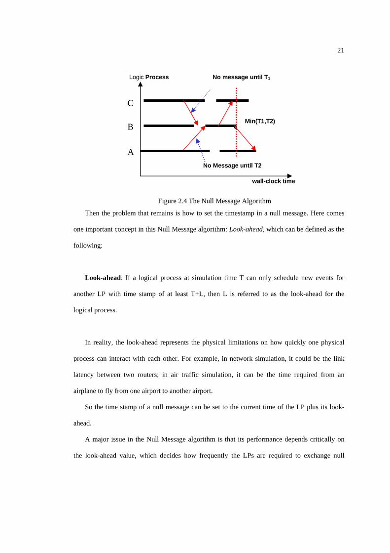
the simulated systems. As shown in Figure 2.4, a null message with timestamp T1 from LP C to
LP B promises that no events with timestamp smaller than T1 will be sent from LP C. After LP
B receives all null messages from all other LPs, LP B can figure out what the upper bound of
the timestamp is, and all events with smaller timestamps can be processed safely. In this case,
all events with timestamp less than Min(T1, T2) can be processed safely.
21
wall-clock time
Logic Process
A
B
C
No message until T1
Min(T1,T2)
No Message until T2
Figure 2.4 The Null Message Algorithm
Then the problem that remains is how to set the timestamp in a null message. Here comes
one important concept in this Null Message algorithm: Look-ahead, which can be defined as the
following:
Look-ahead: If a logical process at simulation time T can only schedule new events for
another LP with time stamp of at least T+L, then L is referred to as the look-ahead for the
logical process.
In reality, the look-ahead represents the physical limitations on how quickly one physical
process can interact with each other. For example, in network simulation, it could be the link
latency between two routers; in air traffic simulation, it can be the time required from an
airplane to fly from one airport to another airport.
So the time stamp of a null message can be set to the current time of the LP plus its look-
ahead.
A major issue in the Null Message algorithm is that its performance depends critically on
the look-ahead value, which decides how frequently the LPs are required to exchange null

22
messages. As we know, null messages do not represent any useful activity in the simulated
systems and are pure simulation overhead.
Global barrier
Wall-clock time
Logic Process
A
B
C
Figure 2.5 Synchronous using Barrier Synchronization Protocols
The Null Message algorithm can be implemented efficiently using a mechanism called
barrier synchronizations. A barrier is a general parallel programming construct that defines a
point in time when all the processors participating in the computation must stop. As shown in
Figure 2.5, before a LP process enters the barrier, it sends null messages to other LPs; then it
blocks and waits until it receives all null messages from the other LPs. The barrier operation is
completed when all LPs have received all null messages, and then the LP is allowed to resume
execution until the next barrier point, which is the current time plus look-ahead.
Up-goingNull message
Down-going Null message
Figure 2.6 Global Barrier using a Tree Structure

23
The benefit of using a barrier is that we do not have to send null messages between all pairs
of logical processes. Instead, we can organize the logical processes efficiently and reduce the
number of null messages greatly. If, the logical processes are on a shared-memory
multiprocessor, the barrier can be easily achieved by using a global synchronization variable. If
the logical processes are on a distributed system like a cluster, all LPs in a machine can
synchronize locally and then use a representative to synchronize with other machines. The
machines can be organized as a balanced tree with each node of the tree representing a different
machine (Figure 2.6). When a leaf machine reaches the barrier points, it sends a null message to
its parents. Each machine will wait until it gets all null messages from its children and then send
a null message to its own parent. After the root receives all outstanding null messages, it knows
every machine has entered the barrier. And this information can be propagated back to all
machines following the revert tree.
2.3 Graph Partitioning
Our work exploits graph partitioning algorithms as a key tool in solving critical load
balance problems, necessary to provide scalability for our network simulator
2.3.1 Single-Objective Single-Constraint Graph Partitioning
Problem
Typical graph partitioning algorithms generally solve single objective partition problems
such as:
Given an input graph G = (V, E) with weighted vertices and edges, we want to partition it
into k parts such that,
- each part has roughly the same number of vertex weight (constraint)
- the edge-cut (the number of edges) that straddles partitions is minimized (objective)

24
The task of minimizing the edge-cut is considered as the objective and the requirement that
the partitions will be of the same size is considered as the constraint. This single-objective
single-constraint graph partitioning problem is can be efficiently solved with multi-level k-way
graph partitioning algorithms[39], and it is widely used for static partitioning in scientific
simulation.
2.3.2 Multi-Constraint Graph Partitioning Problem
However, this single constraint graph partitioning problem is not sufficient to model many
of the underlying computational requirements, found in today’s large scale applications. For
example, in a large distributed application, we need to balance both the computation load, as
well as the memory consumption, across multiple physical nodes. Both memory and
computation are two distinguished constraints, and if the partitioner fails to balance both
requirements, it is hard to achieve good overall application performance. This problem can be
solved by modeling it as a graph in which every vertex has an associated weight vector w of
size m, every weight represent an balance requirement, every edge has a scalar weight, for
which we find a partitioning such that each partition has roughly equal vertex weight with
respect to each of m weights and the edge-cut is optimized. This problem is usually referred to
as the multi-constraint graph partitioning problem, and there are many efficient algorithms
available [40, 41].
2.3.3 Multi-Object Graph Partitioning Problem
Beside multiple balance requirements, a complex distributed application may have multiple
optimization requirements. For example, a multi-phase application can consist of multiple
phases; each phase has quite different communication patterns. If we want to minimize the
communication traffic across the network, we should put multiple phases together, and balance
the requirement of different phases. This problem can be solved by modeling it as a graph in

25
which every edge has an associated weight vector w of size m, each weight represents an
optimization requirement, every vertex has a scalar weight, and for which we find a partitioning
such each partition has a roughly equal amount of vertex weight and the edge-cut with respect
to each of m weight and the edge-cut is optimized. This problem is usually referred to as a
multi-objective problem, and there are some efficient algorithms to solve it [42].
There have been a large number of graph partitioning packages targeted at parallel
computing since the early 90’s, including METIS[42], Chaco[43], Jostle[44], PARTY[39], and
Zoltan[45]. As a well studied problem, we expect that any high quality graph partitioning
package (in this case METIS[42]) should produce results of comparable partition quality to
other graph packages. Our choice of METIS is mainly due to its performance and the flexibility
in supporting multiple constraints, as well as multiple objectives.

26
Chapter 3 Dissertation Statement
The focus of our research is to enable the study of dynamic interaction between applications,
middleware, resources, and networks in a controlled environment. We first describe the
hardware and software context for this dissertation in Section 3.1, and then we define the
simulation problem in this context in Section 3.2. Our dissertation statement is given in Section
3.3, while Section 3.4 discusses the way to evaluate our approach.
3.1 Context
First, we introduce applications which are the subjects of our performance study. And then
we describe the software and hardware resources to be used for the study.
3.1.1 Target Applications, Networks, and Resources
In the last few decades, the prospects of large-scale distributed applications deployed across
the Internet have grown phenomenally. Examples of those applications include distributed
supercomputing applications, peer-to-peer file sharing application, distributed interactive
simulation (DIS) for training and planning in the military, and real-time widely distributed
instrumentation systems[5]. These applications often involve thousands of geographically
distributed endpoints (including computers, storages, and instruments) connected through wide
area networks with latency ranging from a few milliseconds to a few hundreds milliseconds.
They are sufficiently coarse-grained that they can run on the Grid, but their performance greatly
depends on network conditions, such as traffic congestion and routing stability. When compared
to traditional parallel and distributed computation in a local area network, the conditions of

27
wide area network show much larger variability and therefore lead to much more unstable and
unpredictable performance. Moreover, resource hungry large applications can not only affect
the network performance with their multi-gigabit traffic streams, but may also be network aware
and respond to current network performance. Therefore, it is critical to study the application
behavior under different network conditions.
These applications often have complex logic, coupling large computation and storage
resources. They can also be built above grid middleware, such as Globus[5], Legion[6], and
Condor[7]. Furthermore, with help from emerging grid software tools, such as the Network
Weather Service (NWS)[23] and GrADS developing framework[9], more applications can
adapt to the available network and resource conditions for better performance. All these
components together make a complex system which may exhibit non-linear dynamic behavior,
and depend on some subtle interactions between multiple components.
It is very important to understand the performance and behaviors of these applications under
grid environments. It can be used to predict the application performance before deployment,
decide the resource requirement for predicted performance, diagnose the system abnormality
after deployment, and detect the system performance bottleneck for upgrading.
3.1.2 Execution Platform
In order to understand these applications, we need an execution platform for simulation
experiments. First of all, the platform hardware and available software should be scalable in
order to support large scale simulation. Second, the cost effective is also an important criterion,
since it decides whether or not the platform will be widely available. In our study, we choose
the cluster platform, based on the following considerations.
First, clusters have become a cost effective and popular way to build large-scale systems.
The low latency cluster communication hardware and software (like Myrinet and MPICH-GM)

28
have improved their performance greatly. These days, most supercomputers are built on cluster
technology, and small clusters are widely available in research communities. Large scale SMP
machines are too expensive for most researchers.
Second, also for cost reasons, cluster systems usually have more memory than SMP
machines. It is normal for a 64-node cluster to be equipped with 256GB memory, which is
comparable to the 288GB memory of the high end Sun Fire 12K Enterprise Server [46]. Since
most simulations require a great deal of memory, cluster systems present a big advantage over
SMP based parallel simulation.
Third, using flexible cluster technology is often easy to achieve large network throughput.
For online network simulation, the simulation engine needs to exchange network traffic with
applications running on other machines. An SMP machine usually has very high inter-processor
bandwidth, but the external network I/O is usually quite limited, since only a few I/O processors
can process external network traffic. This may quickly become a bottleneck for the whole
simulation system. Cluster systems, on the other hand, are quite different. With current network
switches, the application traffic can be easily handled by every simulation node and efficiently
distributed to different nodes for better load balance.
Our target cluster is one that can fit in a single room and is entirely connected by at least
one high performance network, such as switched Fast Ethernet or Myrinet. Bandwidths of the
network range from 100Mbps up to 10Gbps, and the network latency for small message should
be around a few microseconds. In addition, our target cluster should have TCP/IP protocols and
a high performance MPI implementation available, such as MPICH-GM. The MPI is primarily
used for the communication within the distributed network simulation.

29
3.2 Problem
To meet the challenge outlined above, integrated simulation tools are required for modeling
virtual grid systems. The questions are how to do it, how to do it accurately, and how to do it
efficiently with high scalability.
3.2.1 How to Provide a Virtual Gird Environment
A virtual grid environment should be fully virtualized, which means applications can be
executed on the virtual grid without any modification, they should use all virtual resources,
storage, and networks transparently. This is important to maximize the range of experiments
and their realism. Compared to traditional emulation systems, which also support directly
execution of real applications, a virtual grid environment is more complex because it must
support virtual resource identification, virtual resource discovery, and virtual resource
interaction. It is critical to use real applications and middleware transparently; it is also required
in order to enable the direct study of dynamic interactions between applications, middleware,
resources, and networks.
For example, in a typical Globus application, one may use the GIS system to discovery
suitable resources first, and then submit the job to multiple gatekeepers, which launch jobs on
local resources through job-managers. There are many open questions with regards to
supporting Globus application transparently, they include: How do we describe and discover
virtual resource in the GIS system; how do we associate virtual resources with gatekeepers; and
how are applications launched from job-managers on virtual resources.
3.2.2 How to Simulate Efficiently and Accurately
Although highly accurate simulations are always desirable, with limited physical resources
one must make tradeoffs between accuracy and efficiency. For example, there are accurate

30
simulators for processor, memory, and disks. But if those simulators were used for grid
modeling, they would take too much time to yield any results, despite their accuracy. On the
other hand, the resource simulation must be accurate enough in capturing the underlying details
for it to be useful. For example, in a peer-to-peer application, it requires hundreds of endpoints
to build a representative overlay network structure.
So the first question to ask is how much accuracy is required for a specific resource
simulation, or could we reduce the accuracy requirement without hurting the overall accuracy of
the whole simulated system. For example, do we need packet level detail for network simulation,
and do we need the instruction level simulation for computation resource modeling. After this,
we should determine how to simulate it efficiently. Our choices may include how to simplify
the routing protocol in simulation without affecting the final routing decisions, or how to
aggregate the simulation of a large number of idle virtual resources with a single physical
resource. This decision making is critical to achieve accurate modeling of a virtual grid, in a
timely manner, given the bounds of physical resource constraints.
3.2.3 How to Simulate with High Scalability
Another challenge in modeling grid dynamics is the scalability of the simulation tools.
Essentially this means, can the simulation tool use physical resources efficiently and also, can it
support simulation of larger networks or applications when more resources are available. This
challenge is decided by both the scale of the Internet itself, which includes millions of hosts and
routers, and the scale of grid applications, which usually consist of hundreds and thousands of
processes distributed across a wide area network. To make a meaningful grid simulation, it
should be able to support a network comparable to a significant part of the real Internet, with
reasonable background traffic; it should also be able to support real applications with thousands
of endpoints.

31
In Grid simulation, the scalability issue is particularly critical for the network simulation.
The other components, such as computing nodes and storage systems, can be simulated in
parallel given enough computing resource. However, these components need communication
and coordination to function correctly, which in a distributed simulation happens through the
network system. Due to small network delay and fast interaction among network routers and
endpoint hosts, the whole network systems must be simulated with enough concurrency and
tight synchronization.
Beside the implementation efficiency we mentioned above, there are two major factors
affecting the scalability of a distributed simulation system. First, scalability depends on
available parallelism, and thus, the problem is whether and how to find large parallelism for a
given network simulation. There is significant on-going research on parallel and distributed
network simulation. Some of these solutions exploit the parallelism in network simulation on
SMP machines, but they suffer from limited internal hardware scalability. Only a few recent
simulators support exploiting scalable message passing systems, such as a cluster system.
However, none of them have demonstrated good scalability when challenged with irregular
network simulation problems. This is due, mainly, to the fact that the communication overhead
on cluster systems is much larger than that of SMP machines, and thus, it requires more
parallelism in the simulation problem itself, in order to achieve good performance.
Second, scalability depends on the achieved load balance. Load balance is important
because it directly affects the simulation performance: the speed of the parallel/distributed
simulation is limited by the speed of the node with the most loads. How to achieve load balance
across simulation engine nodes is still an open research problem. Since the simulation engine
load depends predominately on the amount of simulated traffic, which may change dramatically
during the simulation, balancing the simulation load is a big challenge. Our choice of cluster

32
platform also makes load balance more difficult, since it basically rules out the possibility of
dynamic load balance, due to the high overhead of task migration across machines.
3.3 Dissertation Statement
My thesis is:
Accurate and comprehensive study of the dynamic interaction of applications, middleware,
resources, and networks is important and is possible with scaled real-time online network
simulator. Using sophisticated load balance algorithms by exploiting a range of static network
and dynamic application information, distributed network simulation based on discrete-event
simulation engine can be scalable and support high fidelity simulation of a large grid system.
Scaled real-time simulation is our approach to enable hybrid simulation of multiple
simulation modules. As we argued in the last section, it is essential to model multiple resources
and network together for modeling dynamic interaction of applications, middleware, resource,
and networks. Scaled real-time simulation is a special kind of simulation in which simulation
time advances with constant rate, usually slower than real-time. It is different from traditional
simulation and emulation approaches in the way the simulation time advances: in traditional
simulation, the simulation time advances as fast as possible, and in emulation approaches, the
simulation time advances just as real time. Our approach relaxes this real-time requirement of
emulation and allows more flexible resource speeds and ratio. Scaled real-time simulation is the
base of coordinating multiple hybrid simulation modules without complex synchronization
mechanism.
Online network simulation is our approach to improve the simulation accuracy. It is an
enhanced network simulation technology, which can pass live traffic from application through
the simulated network to its destination, and support direct application execution. Thus, online

33
network simulation allows the study of real, temporal and feedback behavior of network and
application protocols, as well as their interaction with other network traffics. The scaled real-
time online network simulation technique, plus other resource modeling and virtualization
methods, can provide accurate simulation of virtual gird environments.
To support large-scale simulation, the key speed limits are the simulation efficiency and the
load balance of distributed network simulation. The load balance problem is known to be hard,
since simulation workload is proportional to network traffic packet number, which changes
dramatically with bursts of traffic loads in large network. The characteristics of grid
environment with highly distributed applications and complex dynamic interactions between
applications, networks and resources make the problem even harder. Our sophisticated load
balance algorithms exploit a range of static network and dynamic application information to
improve the load balance. Good load balance is important for the performance of the network
simulation and therefore for the scalability of the entire virtual grid model.
3.4 Success Criteria
To demonstrate that our scaled real-time online simulation technique can successfully
enable hybrid simulation of multiples resources and application together, we need to present our
design and implementation. Success will be demonstrated by providing a simulation toolkit
which can provides modeling of virtual grid environment. Using this simulation toolkit, we will
construct a range of grid environments and execute a batch of real applications directly on the
simulated grids.
In addition to the support of direct application execution on virtual grids, fidelity is also an
important success criterion. For fidelity, the basic question is whether we have developed a
simulation mechanism that can provide detailed and accurate modeling of the virtual grid.
Success will be demonstrated by a range of validation experiments. We will first provide

34
validation on the accuracy of single resource modeling, including network and computation
resource. The validation experiments will show that the network simulator achieves correct
network latency and bandwidth under multiple network configurations and that the computation
resource simulation enforces the correct resource usage under multiple resources and
application configurations. Then we will validate that for a given real application, the modeling
is still accurate. The basic methodology is to use the MicroGrid to simulate a few real systems,
and then, compare the application performance on real systems directly to that on the simulated
systems. The application execution time between the real systems and the simulated systems
should match.
Using advanced load balance algorithms to achieve good scalability is also a critical claim
in our dissertation statement. Success will be demonstrated by designing and implementing
those load balancing algorithms, applying them on experiments with a range of network
topologies and application configurations, and improving the scalability of the whole simulation
systems in the term of load imbalance, application simulation time, and parallel efficiency (see
Section 7.1.3 for detailed metrics definition).
We will also show that the scalability we achieve is good enough for detailed grid modeling.
Success will be demonstrated by executing simulations of Grid applications over large network
systems, including a simulation of a large ISP network with 20,000 routers and hosts, a
simulation of the real Internet BGP simulation of more than 16000 Autonomous Systems, and a
simulation of a large scale Denial of Service attack on an 200-node overlay network with 200
users and 10Gbps of attacking traffic. We set these scale thresholds (network size, application
number, traffic volume, etc.) because we think they are large enough to keep the major feature
of a large grid environment and that the simulation results are applicable to real grid
environments.
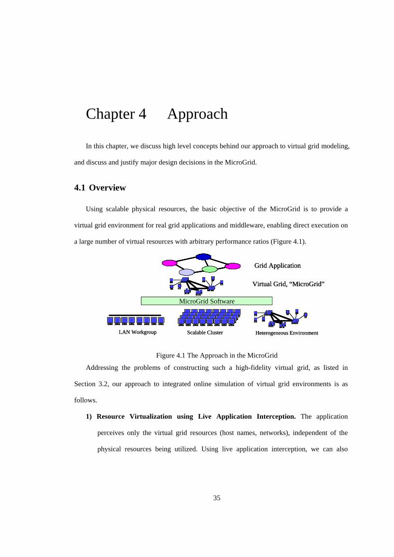
35
Chapter 4 Approach
In this chapter, we discuss high level concepts behind our approach to virtual grid modeling,
and discuss and justify major design decisions in the MicroGrid.
4.1 Overview
Using scalable physical resources, the basic objective of the MicroGrid is to provide a
virtual grid environment for real grid applications and middleware, enabling direct execution on
a large number of virtual resources with arbitrary performance ratios (Figure 4.1).
Figure 4.1 The Approach in the MicroGrid
Addressing the problems of constructing such a high-fidelity virtual grid, as listed in
Section 3.2, our approach to integrated online simulation of virtual grid environments is as
follows.
1) Resource Virtualization using Live Application Interception. The application
perceives only the virtual grid resources (host names, networks), independent of the
physical resources being utilized. Using live application interception, we can also
Grid Application
Virtual Grid, “MicroGrid”
MicroGrid Software
LAN Workgroup Scalable Cluster Heterogeneous Environment
Grid Application
Virtual Grid, “MicroGrid”
MicroGrid Software
LAN Workgroup Scalable Cluster Heterogeneous Environment

36
virtualize the grid information services and virtualize/simulate the appropriate operating
system resources.
2) Computation Resource Simulation using Soft Real-time Scheduling. The target is to
achieve accurate computation resource modeling with less overhead and less
prerequisites. Based on direct application execution and user level process scheduling,
the soft real-time scheduling approach can efficiently model a large number of virtual
resources on a single physical host.
3) Network Modeling using Scalable Online Simulation. To improve the scalability of
virtual grid modeling, the traffic-based load balance for distributed conservative
discrete-event network simulation is used. The distributed simulation can exploit
parallelism in the network simulation problem, and our sophisticated load balance
algorithms can use a range of network and application information to achieve good load
balance and performance of the entire simulation.
4) Coordination of Multiple Simulation Modules using Scaled Real-time Execution. To
provide a coherent global simulation of multiple virtual resources, we need to
coordinate the simulation speed of different virtual resources. This can be achieved
through scaled real-time execution of all simulation modules. Based on the desired
virtual resources and physical resources employed (CPU capacity and network
bandwidth/latency), the virtual time module determines the maximum feasible
simulation rate, under which all resource simulation can be run in a functionally correct
manner.
We will discuss these approaches in detail in the following sub-sections.

37
4.2 Resource Virtualization using Live Application Interception
To virtualize a grid environment, the MicroGrid intercepts all direct uses of resources or
information services made by the application. In particular, it is necessary to mediate over all
operations which identify resources by name, either to use or retrieve information about them.
We first consider general mediation, and then we consider the specific issue of information
service.
4.2.1 Virtualizing Resources
Hardware
Virtual Machine Monitor
OS OS
APP APP
OS
APP
Figure 4.2 Virtualization based on VMM
Virtualization, in a rather loose definition, is a framework that devides the resources of a
computer into multiple execution environments. More specifically, it is a layer of software that
provides the illusion of a real machine to multiple instances of virtual machines. In general,
there are two possible ways to virtualize resources. The first approach is the virtual machine
monitor (VMM) approach (Figure 4.2), including VMWare[47], Denali[48], Entropia[12], and
Xen[49]. VMMs usually provide full virtualization, while a guest operating system instance is
required to provide a virtual machine on which traditional applications can be directly executed.
However, the complexity and overhead of VMMs is so large that it is infeasible to create many
instances on a single physical machine. For example, the CPU performance loss of VMWare is

38
between 9-15%. Also, VMMs have little support for virtual network performance modeling,
which we will discuss in Section 4.3.
Hardware
Shared OS
App with Virtual ID
App with Virtual ID
App with Virtual ID
Figure 4.3 Virtualization based on Virtual Host ID
Another approach is to just virtualize the host identity (Figure 4.3). In general, we need to
virtualize processing, memory, networks, disks, and any other resources being used in the
system. However, since operating systems effectively virtualize each of these resources --
providing unique namespaces for each process and sharing of CPU, disk, etc-- the major
challenge is to virtualize host identity. The benefits of this approach are the simplicity and
efficiency; consequentially, it can be naturally used for virtual network performance modeling.
This approach is especially good if one wants to create a large number of virtual hosts, but
maybe only a small part of them are active at the same time. The idle virtual machines basically
introduce no overhead to the physical machine, a feature quite different from that of the VMM
approach. Of course, this requires added resource modeling to guarantee correct virtual resource
performance.
In the MicroGrid, we choose the virtual host identity approach, since we intend to simulate
a very large number of virtual hosts. Each virtual host is mapped to a physical machine using a
mapping table of virtual IP address to physical IP address. All relevant library calls are
intercepted and mapped from virtual to physical space using this table. These library calls
include:
gethostname()
39
bind, send, receive (e.g. socket libraries)
process creation
By intercepting these calls, a program can run transparently on a virtual host with the
appearance of the virtual hostname and IP address. The interception ensures that the program
can communicate with processes running on other virtual Grid hosts. Many program actions
which utilize resources (such as memory allocation) only name hosts implicitly, and thus, do not
need to be changed. Any socket-based application can be run on the virtual Grid as the
MicroGrid completely virtualizes the socket interface.
4.2.2 Virtualizing Information Services
Information services are critical for resource discovery and intelligent use of resources in
Computational Grids. To provide a fully virtualized Grid environment, we also need to provide
information services for virtual resources. For example, when it comes to supporting the Globus
middleware, this problem amounts to virtualization of the Globus Grid Information Service
(GIS)[50].
One key problem is how to get application to look at the virtual information service. One
straightforward solution is to run an information service in the virtual world, and store and
retrieve all virtual resource information directly. This is a simple solution in logic, but it
introduces a large overhead in experiments. For example, in Globus, this requires a GIS server
for every experiment, it takes significant time to initialize the GIS server, and makes it hard to
add simulation-related information.
Instead, our approach is to use a real information server --- no additional servers or
daemons are needed. In this approach, an application running in the simulation environment
needs to talk to a server in the real world, and it requires special support from the network
virtualization module. The network virtualization module should intercept all access to network,

40
identify all access to virtual information services, and forward them to the real information
server directly, instead of routing through the network simulator.
Beside this transparent access issue, desirable attributes of a virtualized information
services include:
1) Compatibility: virtualized information should be used as before by all programs
2) Identification and Grouping: easy identification and organization of virtual Grid entries
should be provided
3) Use of identical information servers: there should be no incompatible change in the
entries
Our approach achieves all of these attributes by extending the standard GIS LDAP records
with fields containing virtualization-specific information. Specifically, we extend records for
compute and network resources. Extension by addition ensures subtype compatibility of the
extended records (a la Pascal, Modula-3, or C++). The added fields are designed to support
easy identification and grouping of the virtual Grid entries (there may be information on many
virtual Grids in a single GIS server). Figure 4.4 and Figure 4.5 show examples of the
extensions to the basic host and network GIS records.
hn=vm.ucsd.edu, ou=CSAG, ...
Is_Virtual_Resource=Yes
Configuration_Name=Slow_CPU_Configuration
Mapped_Physical_Resource=csag-226-67.ucsd.edu
CpuSpeed=10
Figure 4.4 Virtual Host MDS Records

41
nn=1.11.11.0, nn=1.11.0.0, ou=CSAG
Is_Virtual_Resource=Yes
Configuration_Name=Slow_CPU_Configuration
nwType=LAN
speed=100Mbps 50ms
Figure 4.5 Virtual Network MDS Records
4.3 Computation Resource Simulation using Soft Real-time
Scheduling
To provide accurate virtual grid modeling, the MicroGrid need to simulate every
computation resource as a component of the overall simulation, providing real-time
performance feedback to the simulation and regulating the rate at which virtual time is allowed
to progress. The major challenge in computation resource simulation is that we need to simulate
a large number of resources efficiently, due to the fact that a typical grid environment usually
includes thousands or more resources which need to be simulated in a much smaller cluster
system.
One possible solution to the above challenge is using the VMMs in Section 4.2, which also
provide computation modeling for virtual machines. This approach is accurate but involves
more overhead. Another possible approach is to use real-time operating systems to schedule the
execution of virtual machines, which can be more accurate, but less flexible, since real-time
operating systems are not widely deployed.

42
CPU Controller
Virtual Machine
APP
APP
APP
Virtual Machine
APP
APP
Virtual Machine
APP
APP
APP
Physical Machine
Figure 4.6 Computation Resource Simulation using Soft Real-time Scheduling
Based on the direct execution of application and resource virtualization, computation
resource simulation is to provide appropriate performance for the processes running on a virtual
compute resources. As shown in Figure 4.6, the MicroGrid uses a CPU controller, a soft real-
time process scheduler, on each physical host to control resource utilization of the processes
resident with each virtual machine. Periodically, the controller checks the CPU usage of every
application process on the physical machine, and then calculates the latest CPU usage of each
virtual host. If the amount of effective cycles exceeds the speed of the virtual hosts, the
controller stops all processes of that virtual host; otherwise, the controller wakes up the
processes and lets them proceed.
In theory, this approach can accurately simulate an arbitrary number of virtual computation
resources by tuning the simulation speed. However, due to the limitation of non-real-time
operating systems and minimal OS scheduling unit, the CPU controller can neither accurately
monitor the real resource usage of every application process, nor stop and wakeup a special
process at the exact points it should. We will discuss in more detail how to address this issue in
Section 5.2.

43
To summarize, our computation resource simulation approach is to use direct execution on
original operating system, and control the overall CPU time allocated to a specific virtual
machine. This light-weight approach is efficient and can support a large number of virtual
machines on a physical machine. Moreover, it is flexible, and can be used on any target
operating system of the real application. One major short-coming to this approach is low
accuracy, since it does not guarantee resource usage from the bottom line. However, as you will
see from the validation experiments in Section 6.1, the accuracy is sufficient for most
application simulation.
4.4 Network Modeling using Scalable Online Simulation
There are critical challenging requirements for network simulation in the MicroGrid:
accuracy, scalability, and support for direct application execution, and they are addressed in
Section 4.4.1, Section 4.4.2, and Section 4.4.3, respectively.
4.4.1 Packet Level Detailed Simulation
While significant advances have been made in aggregate modeling of network behavior[20,
21], at present only detailed packet-level or close analogs can model protocol dynamics
accurately, particularly in extreme cases[23]. This is especially true when we target our study on
application performance. Extreme cases are important. Since while they rarely happen in normal
operation, their consequence may be critical. For examples, for a distributed application, what is
the performance with routers in link saturation as happens under malicious Denial-of-Service
attacks? How could the routing system respond if there is temporary network partition due to
attacks?
Remember that we want to understand the behavior of individual applications, we want to
understand and diagnose anomalies, and we also want to understand behavior of collections of
applications and resources in ordinary and extreme circumstances. For all these purposes, the

44
details matter. Since network and application behavior depends on detailed packet behavior, and
feedback effects on network protocols and resource management are critical, the simulation
must use closed-loop feedback.
To capture as many as possible network protocol details, packet level simulation is required
to provide accurate modeling. For example, it is known that most applications use the TCP
protocol for network communication and their performance directly depends on the behavior of
TCP. However, TCP performance is sensitive to individual packet behavior. For instance,
whenever a TCP sender detects packet loss, it will reduce the congestion window size by half,
thus reducing the TCP bandwidth dramatically. Congestion window increase, which is additive,
takes a longer time to recover. Another example is the Nagel Algorithm[51] in TCP, which is
used to delay the sending of small data until more data are available, because sending large
packets has less overhead. However, this optimization may raise major performance issue for
interactive or RPC-based applications.
4.4.2 Online Network Simulation
Simulation Engine Progress as fast as
poissible
Network Model
Simple Application
Model
Real Application
Traffic Reference
Real Traffic
User Interface
Simulation Engine with Constant Rate
Network Model
SimulationInterface
Traffic Reference
User Interface
Figure 4.7 Online Network Simulation vs. Network Simulation
Network simulators, such as the NS-2, have been widely used to study network protocol
and network performance for a long time. Usually these tools focus on the network itself, and

45
they cannot be used to study application directly. The user must write a simulation module to
abstract and mimic the behavior of the application. It requires deep understanding of the
application to write such a performance module effectively, and it invariably introduces
unknown inaccuracy through this approximation and abstraction. With the coming of complex
distributed and Grid application, it becomes less and less feasible to write accurate application
modules for simulation. Instead, people want to study applications directly using an online
network simulation, an enhanced network simulation technology which can support direct
application execution by passing and modeling the behavior of live traffic from application
through the simulated network to its destination.
The MicroGrid supports direct execution of real applications to exercise complex
applications and to capture the subtle interaction between applications, middleware, and
operating systems. Just like the virtualization of network identity, the MicroGrid intercepts all
network related function calls in a given application, and redirects the traffic into the network
simulator. The packet movement and timing are modeled by the network simulator and the data
are feed back to real application at the other endpoint at the correct time (Figure 4.7). Here the
MicroGrid provides a virtual Grid environment and the user can use it as a real Grid testbed
transparently. We call this approach online network simulation.
The benefit of online network simulation is that the user can study application performance
directly, rather than building another application module for the simulation. This reduces the
overhead of simulation greatly, and since it catches all the details of the application
implementation as well as interactions between the application and the real system, it provides
more accurate and direct results to the users.
There are two major challenges in online network simulation. First, we need to intercept the
network traffic transparently; second, the delay between the application and simulator must be

46
negligible when compared to the simulated network delay, since this delay is not modeled by
the simulator. We will discuss this in more detail in Section 5.3.
There is another technique that has an objective similar to online network simulation, but
uses a different approach, called network emulation. Like online network simulation, network
emulation also supports direct application execution and intercepts the live application traffic
transparently. However, instead of using a network simulator, it usually uses software or
simulated routers to approximate the network behavior. The benefit of this approach is the raw
speed it offers. This approach often allows for emulation that is fast enough for real-time
execution. However, accuracy and flexibility are usually limited when compared with online
simulation.
4.4.3 Distributed Conservative Discrete Event Network Simulation
Here we describe and justify some of our design choices in network simulation.
4.4.3.1. Parallel vs. Distributed Simulation
To provide scalable large-scale simulation, we can use parallel discrete-event simulation.
Over the last two decades, parallel discrete-event simulation, or PDES for short, has been
recognized as an important and challenging research area. PDES is used when executing a
single discrete-event simulation program on a parallel computer, which can be either a shared-
memory multi-processor or a distributed-memory cluster of computers. By exploiting the
parallelism inside a simulation problem, parallel simulation overcomes the limitation of
memory and execution speed of sequential simulation. We can find in-depth review of the state
of art of PDES in the Fujimoto book[52].
In general, parallel simulation on shared memory machine is a much mature approach and is
expected to provide good performance, which is due primarily to simple programming model
and small communication overhead. However, distributed simulation on clusters using message

47
passing communication could be a better choice for large scale network simulation, based on
the following consideration.
First, clusters have become a cost effective and popular way to build large-scale systems.
As we mentioned in Section 3.1.2, clusters are widely available for researchers. Second, clusters
are more scalable than SMP systems. Currently all the largest supercomputers are based on the
clustering technology and some of them are available for public accesses in national computer
center, such as NCSA and SDSC. This provides the opportunity for extreme large-scale network
simulation. Third, the coming of advanced distributed simulation technology, including DaSSF,
enables a chance to build large scale network simulators based on distributed simulation.
4.4.3.2. Conservative vs. Optimistic Simulation
Conservative algorithms try to avoid any possible causality errors. In practice, they are
usually overly pessimistic, and force sequential execution when it is not necessary. This reduces
the achievable parallelism in the simulation and requires good look-ahead (see Section 2.1) for
concurrent execution and scalability. Optimistic algorithms, on the other hand, allow violation
to occur but provide a mechanism to recover, which can achieve greater parallelism and has no
limit on the look-ahead. However, optimistic algorithms usually have more complex control and
need special mechanisms for state saving, roll back, and dynamic memory allocation.
The preference for different synchronization methods depend on the structure of simulation
events and interaction between simulation entities, which in turn depends on the systems being
modeled. For online network simulation, we prefer the conservative algorithm for the following
reasons.
1) Easier to implement. From our experiments, we can also tell that the look-ahead in
network simulation is sufficient (with good partition algorithms) to achieve good speedup, even

48
when the absolute look-ahead is not very large: the network delay of a physical link (1-10
milliseconds).
2) Smaller memory footprint. In a large network simulation, we need to simulate thousands
of hosts and routers, and an even larger number of network packets. The memory requirements
are critical to the scalability of the whole system. Due to the property of optimistic simulation,
the simulator must keep the un-commit events for possible roll-back. Because of the nature of
high speed network traffic, this memory consumption can easily go out of control and degrade
the benefit of optimistic simulation.
3) More stable progress for real-time execution, which is critical for online network
simulation. The rollback of optimistic simulation may halt the simulation and affect the real
time simulation accuracy.
4.4.3.3. Automatic Load Balance for Scalability
As we discussed in Section 3.2, scalability is an open research challenge for network
simulation. The detailed packet level simulation requirements in the MicroGrid present an even
greater scalability challenge. In a large network consisting of thousands of routers and hosts,
there are a large number of traffic flows. It is a serious challenge to simulate such a large
network, which requires such a huge number of computation and memory resources. There is
already a lot of research going on to improve the scalability of network simulation. But much
of this research uses approximation, for example, reducing the network size by removing non-
bottleneck routers and links[53], relaxing the synchronization requirement[35], or even using
fluid flow to represent traffic[54]. As we have shown in Section 4.3.2.1, details matter and none
of these approximations are suitable for our purpose.
With the constraints above, we want to exploit the parallelism in the original network
simulation problem to improve scalability. Based on the specification of the virtual and the
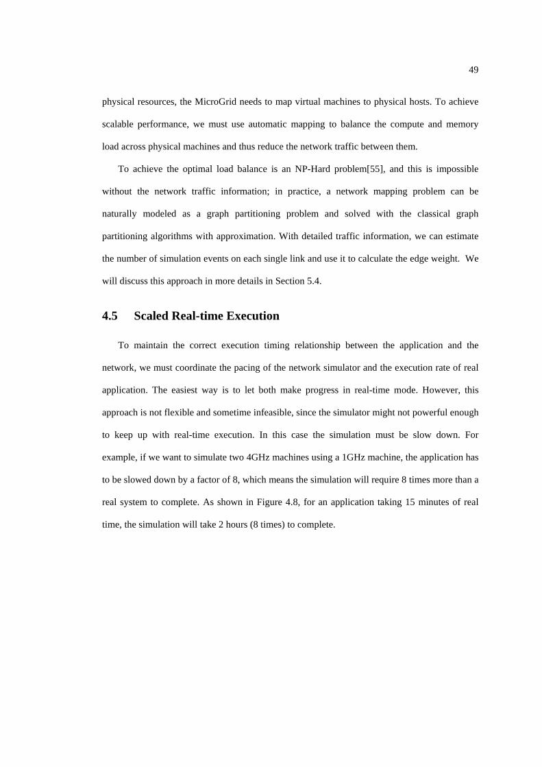
49
physical resources, the MicroGrid needs to map virtual machines to physical hosts. To achieve
scalable performance, we must use automatic mapping to balance the compute and memory
load across physical machines and thus reduce the network traffic between them.
To achieve the optimal load balance is an NP-Hard problem[55], and this is impossible
without the network traffic information; in practice, a network mapping problem can be
naturally modeled as a graph partitioning problem and solved with the classical graph
partitioning algorithms with approximation. With detailed traffic information, we can estimate
the number of simulation events on each single link and use it to calculate the edge weight. We
will discuss this approach in more details in Section 5.4.
4.5 Scaled Real-time Execution
To maintain the correct execution timing relationship between the application and the
network, we must coordinate the pacing of the network simulator and the execution rate of real
application. The easiest way is to let both make progress in real-time mode. However, this
approach is not flexible and sometime infeasible, since the simulator might not powerful enough
to keep up with real-time execution. In this case the simulation must be slow down. For
example, if we want to simulate two 4GHz machines using a 1GHz machine, the application has
to be slowed down by a factor of 8, which means the simulation will require 8 times more than a
real system to complete. As shown in Figure 4.8, for an application taking 15 minutes of real
time, the simulation will take 2 hours (8 times) to complete.
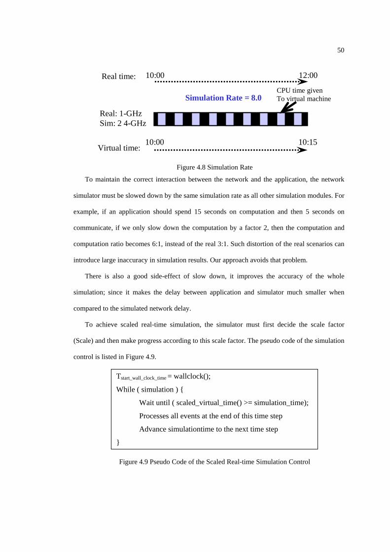
50
Real: 1-GHz Sim: 2 4-GHz
CPU time given To virtual machineSimulation Rate = 8.0
10:00 10:15 Virtual time:
10:00 12:00 Real time:
Figure 4.8 Simulation Rate
To maintain the correct interaction between the network and the application, the network
simulator must be slowed down by the same simulation rate as all other simulation modules. For
example, if an application should spend 15 seconds on computation and then 5 seconds on
communicate, if we only slow down the computation by a factor 2, then the computation and
computation ratio becomes 6:1, instead of the real 3:1. Such distortion of the real scenarios can
introduce large inaccuracy in simulation results. Our approach avoids that problem.
There is also a good side-effect of slow down, it improves the accuracy of the whole
simulation; since it makes the delay between application and simulator much smaller when
compared to the simulated network delay.
To achieve scaled real-time simulation, the simulator must first decide the scale factor
(Scale) and then make progress according to this scale factor. The pseudo code of the simulation
control is listed in Figure 4.9.
Tstart_wall_clock_time = wallclock();
While ( simulation ) {
Wait until ( scaled_virtual_time() >= simulation_time);
Processes all events at the end of this time step
Advance simulationtime to the next time step
}
Figure 4.9 Pseudo Code of the Scaled Real-time Simulation Control

51
This capability can be used to simulate future networks or processors which are much faster
connected to slow 100Mbit networks, future 100Gbit networks, and every speed in between.
For example, by slowing the simulated speed of computing resources, the effect of future high
speed transparent optical networks can be studied.
4.6 Summary
In this chapter, we introduced the MicroGrid approach to modeling the dynamic interaction
between applications, middleware, resources, and networks. To address the challenge of
modeling complex grid applications, Section 4.2 and Section 4.3 present possible solutions
based on live application interception and controlled direct execution. Section 4.4 focuses
mainly on how to achieve accurate and scalable online network simulation. Accuracy is
guaranteed through packet level detailed simulation. To address scalability issues, the basic
approach is to use a distributed conservative discrete event simulation engine to exploit the
parallelism available in the network simulation problem. Section 4.5 addresses the issue of
scaled real-time execution. This is the base of coordination between multiple simulation
modules. And the ability to control resource and network speeds in an online simulation (as
opposed to emulation) enables the MicroGrid to support arbitrary performance ratios between
elements in a simulation.

52
Chapter 5 System Design
The main capability of the MicroGrid is to allow grid experimenters to directly execute
their applications in a virtual grid environment. The MicroGrid can exploit either homogeneous
or heterogeneous physical resources. This chapter describes the MicroGrid 2.4.5
implementation, released in June 2004 and available from http://www-csag.ucsd.edu/. The
MicroGrid 2.4.5, the latest in a series of MicroGrid implementations which stretch back as far
as October 2000, supports Grid applications that use the Globus Toolkit 2 middleware
infrastructure.
This chapter is organized as follows. Section 5.1 provides an overview of the MicroGrid
system design. Implementation of the CPU controller for computation resource modeling is
introduced in Section 5.2. Following that, Section 5.3 presents the details of network modeling,
and Section 5.4 focuses on improving the scalability of network simulation using traffic based
load balance.
5.1 The MicroGrid Overview
We have designed and implemented a tool called the MicroGrid which enables accurate and
comprehensive study of the dynamic interaction of applications, middleware, resource, and
networks. The MicroGrid creates a virtual grid environment – accurately modeling networks,
resources, the information services (resource and network metadata). Thus, the MicroGrid
enables users, grid researchers, or grid operators to study arbitrary collections of resources and
networks. Further, the MicroGrid provides transparent virtualization, allowing the direct study
of complex applications or middleware whose internal dynamics are difficult to model

53
accurately. That is, real application software and middleware can be used unchanged and be
executed on arbitrary virtual grid structures. In short, the MicroGrid provides a virtual grid
infrastructure that enables scientific and systematic experimentation with dynamic resource
management techniques and adaptive applications by supporting controllable, repeatable,
observable experiments.
5.1.1 The MicroGrid System View
ApplicationWrapSocket
ApplicationWrapSocket
ApplicationWrapSocket
ApplicationWrapSocket
CPU Controller
ApplicationWrapSocket
ApplicationWrapSocket
VirtualMachine
CPU Controller
….
Physical Host
VirtualMachine
Online Network Simulator
Application WrapSocket Application WrapSocket
Application WrapSocket
Application WrapSocket
CPU Controller
Virtual Machine
Cluster
Figure 5.1 the MicroGrid System View
The MicroGrid provides an online simulation of virtual grid environments transparently,
allowing applications to be run unchanged. At launch, the MicroGrid reads a virtual grid
configuration, and then builds corresponding simulation objects so as to provide the experience
of running on a virtual grid. These simulation objects implement models of network elements,
compute resources, or grid information services. The MicroGrid can implement the virtual grid
simulation using essentially any physical resources, including homogeneous clusters,
heterogeneous grid resources, or even on a single computer. Usually the network simulator uses
a set of cluster nodes and each node is in charge of simulating a section of the virtual network.

54
The application processes run in different virtual machines which can be hosted by another set
of physical resources.
High speed resource simulation is achieved by direct execution of applications and
middleware on virtual machines. A physical machine can host a few virtual machines and uses a
CPU scheduler to control the speed and capacity of the virtual machine (Figure 5.1). Direct
execution allows experiments to proceed at near real-time. The MicroGrid uses a wrapper
library which automatically intercepts library functions in user applications, thereby creating
hooks for the virtual grid simulation system. Thus MicroGrid users can run any application on
the MicroGrid by simply re-linking the applications to the “wrapper” libraries; neither changes
to the application and middleware source codes, nor understanding of them are needed.
The network traffic from the applications is redirected to an online network simulator by the
wrapper libraries. Data movement is accurately simulated by the network simulator and
delivered back to the application at the appropriate time to reflect ‘actual’ network behavior.
5.1.2 The MicroGrid User View
Cluster
Application Virtual Grid
User
Mapping
Figure 5.2 The MicroGrid User View
To use the MicroGrid, a user must:
1) Specify a set of virtual resources, including network connectivity and protocols.
a. Network topology (Nodes, including routers and hosts and Network links, link
capacity and link latency)

55
b. Network protocol (Transport protocols -- TCP or UDP and Routing protocols –
OSPF, BGP)
c. Node properties related to communication protocols (e.g. TCP buffer, send window,
receive window, segment size, etc.)
d. Compute (relative CPU speed)
e. Compute Node Connections into the network
2) Specify a set of physical resources to be used for the compute and online network
simulation, which in turn are used to control the deployment of virtual resources to physical
resources.
3) Submit a Grid application as a job on the virtual grid, just like on a real Grid environment
4) Observe the execution of the application, and collect results and performance data
5.2 CPU Controller
CPU Controller
Grid Application
Wrap Socket
Process Table
/proc
Virtual Machine 1
Virtual Machine 2
Virtual Machine 3
Grid Application Wrap Socket
SigStop/SigCont
Figure 5.3 CPU Controller
As mentioned in Section 4.2 the MicroGrid uses one CPU controller on each physical host
to monitor the per process resource utilization of the processes on each virtual machine, and
preemptively schedules them using SIGSTOP and SIGCONT signals (Figure 5.3). Here we

56
provide more implementation details on how to guarantee accurate CPU quotas for every virtual
machine in the controller.
5.2.1 The Challenge
Although the idea of the CPU controller appears simple, there are two factors that make it
complex. First, the POSIX.5 thread scheduling mechanism used in Linux is not a real time
scheduler. Specifically, it has a 10 milliseconds scheduling unit; that is, when ever a process is
scheduled to run, it can use up 10 milliseconds. Second, an application can be a mix of
computation and communication; its running time depends on both the CPU speed and the
network speed. Ideally, the CPU controller and the network simulator can collaborate to make
for a more accurate simulation. However, this would make both the network simulator and the
controller more complex. For simplicity and scalability, it is desired that they operate
independently, while the CPU controller can make scheduling decisions based on the
observations of how much CPU time the application has used.
A naïve implementation, which was used in the first release of the MicroGrid toolkit,
demonstrates the effect of these two factors. The original scheduler starts/stops application
processes periodically. The period is calculated from the CPU speed of a virtual machine and
the number of processes loaded on the virtual machine. For example, if the scheduler is to
control a virtual machine which has allocated 25% of real CPU on which two processes are
running, it will assign each process 10 milliseconds every 80 milliseconds.
This mechanism works fine if the application is computation intensive, but has the
following weakness:
First, it is not suitable for communication intensive applications, which use little CPU
resource and spend most of their time waiting for network messages. If the simulation process is
stopped by the controller just before the arrival of network data, it is not able to respond until 70
57
milliseconds later. This 70 milliseconds latency is purely a simulation artifact and hurts the
simulation accuracy tremendously. Similarly, if a virtual machine has both communication-
intensive and computation-intensive processes, the computation process can easily use up all
allocated CPU slots and leave the communication process hungry. This will also introduce large
communication delay and, potentially, skew message inter-arrival time.
Second, it allocates CPU resource uniformly to every process on a virtual machine, which is
unlikely to happen in the real world. If some processes are waiting for disk I/O or network data,
they will not use much CPU time, while other computation-intensive processes should be able
to take their quotas.
5.2.2 CPU Controller with Sliding Window
From the example above, we can see two key issues for good CPU scheduling. First, to
prevent unwanted communication delay, an application process should always be ready to run if
it has not used up its available CPU slots. Second, a computation-intensive process should be
able to use all of the CPU quota allocated to its virtual machine; other given processes on the
same virtual machine do not take their own slices.

58
decides the sliding window size for every virtual machine
while (simulation is running) {
polls the CPU usage information from the /proc
for (every virtual machine) {
calculates the CPU usage percentage during recent sliding window
if exceeds the CPU quota, then
stops all processes on it
}//end of for
sleeps until next scheduling point
} //end of while
Figure 5.4 Slide Window CPU Controller
To address these two issues, we design the sliding window scheduling mechanism. Instead
of proactively starting/stopping processes periodically, the controller lets the OS schedule all
processes on a given virtual machine freely, and simply monitors their CPU usage in the
background. The scheduler will only stop processes on a virtual machine when they have used
up all the CPU time allocated to them. If the virtual machine has been idle for a while, it can
accumulate some “credits” that allow for quick response following network data arrival or I/O
event completion. To prevent a machine from accumulating too many credits, the controller
uses a sliding window algorithm to track its recent CPU usage. The pseudo code of the CPU
controller is presented in Figure 5.4.
Because Linux schedules processes in 10ms units, called “jiffy”s, the controller uses a
window size measured in the units of jiffies. In order to minimize simulation error, we try to
keep the sliding window as small as possible. Since communication latency may be masked by
scheduling granularity, we determine the minimal sliding window size as follows:

59
Suppose E is the design accuracy error and p is the scaled virtual machine speed (fraction of
physical CPU), the sliding window size (w jiffies), and the available jiffies in a sliding window
n should satisfy:
w = round(n/p) and | 1 – n/(p*w) | < E
For every virtual machine with a given E and p, we can first find the smallest n that satisfies
the
| 1 – (n/p)/round(n/p) | < E
Then we can calculate the sliding window size w, which is the smallest sliding window to
satisfy the accuracy error E (set to 5% in our implementation). For example, if we have a 1GHz
machine, and we want to simulate a 600MHz machine with simulation rate 2, then this virtual
machine should take p=(600/1000)/2 = 30% CPU of this physical machine. So we need to find
the smallest n that satisfies:
| 1 – (10n/3) / round(10n/3) | < 0.05
In practice, since n is usually a small integer, we can just try 1,2,3 ,… in sequence, and stop
at the first number that satisfy the inequation above. Here we can get n equal to 2, and then set
the sliding window size w to round(n/p) = 7.
5.2.3 Discussion
The sliding window mechanism allows simulation of large numbers of machines (100’s to
thousands) on a small number of machines. Further, since each virtual machine has its own
window size, grids with extremes of heterogeneous performance from slow to fast machines can
be modeled accurately on the same physical machine.

60
Stopped by OS
Stopped by Network I/O
Wakeup from Network I/O
Wakeup by OS
Slide Window Size
Process A λ=1/2
Process B λ=1/2
: Process In Execution : Process Stopped
Figure 5.5 Possible Inaccuracy from Large Sliding Window Size
However, reducing E often leads to larger sliding window size, which may lead to
simulation error for applications which have mixed computation and communication. The major
reason for this is that the CPU controller has no idea whether a waiting process is waiting for
network delay, or is just scheduled out by the operating system. For example, Process A and
Process B are supposed to use half of the real CPU on two physical machines. Both of them
stop after using ¼ of the sliding window size time, one due to the network I/O and the other due
to the host OS scheduling. At the ¾ sliding window point, process B is re-scheduled to run by
the OS, and the CPU controller should let it use up the rest of the sliding window. Process A is
also woken-up by the completion of network I/O at the same time, and it should be stopped by
the CPU controller, since it should only use ¼ of the real CPU time due. Currently the CPU
controller cannot distinguish these two cases, and it will always grant another ¼ sliding window
time to Process A.
So under some conditions, we may still have large inaccuracies: such is the case when an
application has mixed computation and communication with some special structures, and the
sliding window size is large in comparison to communication latency. As we will show in our
validation experiments, with reasonable design accuracy error E, this situation rarely happens
and has little effect on overall application performance.

61
5.3 Scaled Real-time Online Network Simulation
Network modeling is achieved by MaSSF. MaSSF (pronounced “massive”) is a scalable
packet-level network simulator that supports direct execution of unmodified applications.
MaSSF consists of four parts.
Simulation Engine
Network Modeling
Virtual Grid
I/O Thread Pool
Input Queue
Output Queue
Agent Nodes
Grid Application Wrap Socket
Virtual/Real IP Mapping Server
Live Traffic
SSF API
Figure 5.6 The MaSSF Scalable Network Simulation System
1) Simulation Engine: MaSSF uses a distributed simulation engine based on DaSSF [56].
It utilizes an MPI-connected cluster system to achieve scalable performance. The original
simulation engine, executable only in pure simulation mode, has been modified to operate in a
scaled real-time mode (as discussed in Section 2.3). This simulator can run in a scaled-down
mode when the simulated system is too large to be executed in real time on the available
hardware. With the global coordination of the MicroGrid, this feature provides extreme
flexibility to accurately simulate a wide range of networks accurately.
2) Network Modeling: MaSSF provides necessary protocol modules for detailed network
modeling, such as IP, TCP/UDP, OSPF, and BGP4. We have built simplified implementations
of these protocols which maintain their behavior characteristics. We also use a network
configuration interface similar to a popular Java network simulator implementation, SSFNet[57],
for user convenience.
62
3) Online Simulation Capability: To support simulation of traffic from live applications,
we employ an Agent module which accepts and dispatches live traffic from the application
wrapper to the online network simulation. Traffic is also delivered to application through the
Agent module.
4) Live Traffic Interception: Application processes use a wrapper library called
WrapSocket to intercept live network streams at the socket level. The WrapSocket then talks to
the Agent module to redirect traffic into the network simulator and vice versa. WrapSocket can
be either statically or dynamically linked to application processes and requires no application
modification.
These components and their relationship are illustrated in Figure 5.6. In the following
sections we will present a more detailed description and rationale for our design choices.
5.3.1 Network Modeling
MaSSF’s goal is to enable detailed modeling and simulation of Internet protocols and
networks. It uses object-oriented simulation components to construct a network, setup network
protocols running on various hosts and routers, and create/accept traffic to be simulated. Traffic
can be created using traffic generation modules or can be imported from live applications.
Network traffic is simulated at the IP packet level and every network packet movement is
represented by a simulation event. MaSSF models the hop by hop movement of IP packets
through the network, including link transfer delay, queuing delay in router queues, and packet
drop. The simulation engine has a scaled real-time scheduler that delivers events at the exact
time specified by the event timestamp. In this way, we can capture link congestion and network
dynamics in the real world.

63
5.3.1.1. Network Protocol Stack
Like the Click Modular Router[58] and SSFNet[57], MaSSF provides a batch of protocols,
such as IP, TCP, UDP, OSPF, and BGP, and some network elements, like hosts, routers, links,
and switches, that can be used to construct a network. For example, a host can be configured
with IP, TCP, and Socket protocols, plus an httpClient traffic generation module or a live traffic
Agent module. A router can be configured with IP, TCP, OSPF modules as an internal
Autonomous System (AS) router and it can also be configured with IP, TCP, BGP modules to
be used as a BGP router. With these basic components provided by MaSSF, users can construct
a network entity using any reasonable module combination. Moreover, users can also write
their own protocol modules for new applications or network protocols.
httpServer Agent
socketMaster
tcpSessionMaster
udpSessionMaster
IP
NIC
Connection to other host or router
Figure 5.7 Protocol Stack for a Host with httpServer and Agent
All protocols running on a host or router are constructed as a protocol stack with well-
defined interfaces to facilitate the data movement along the stack. Figure 5.7 illustrates the
major network elements and protocol sessions that are used in a host model. This host is
equipped with one network interface card (NIC), which is connected to another host or router.

64
The host has an httpServer application running, which uses a socket interface, just like in a real
operating system, to communicate with the TCP protocol session masters at the transport layer.
A TCP or UDP session is created when a request arrives from the application, and is torn down
when the session is finished. An IP layer is required to manage packet sending, receiving, and
forwarding by the NIC. This host also has an Agent protocol module, which means it can accept
real traffic from live applications. Figure 5.8 is a router equipped with two NICs, with both
BGP and OSPF routing protocols.
OSPF BGP4
socketMaster
tcpSessionMaster
IP
NIC
Connection to other host or router
NIC
Figure 5.8 Protocol Stack for a Router Running BGP and OSPF
5.3.1.2. Network Topology and Configuration
The first step in network simulation is to provide the topology and configuration of the
network to be simulated. In MaSSF, the input network is described by the Domain Modeling
Language (DML). MaSSF models are self-configuring - that is, each MaSSF class instance can
autonomously configure itself from a configuration file in DML format [59].

65
DML has a simple syntax: it is a list of attributes. The key of the attribute is an identity and
the value of the attribute can be a number, a string, or another attribute list enclosed in brackets.
DML is a recursively defined list of key-values. Logically, a DML file can be viewed as a tree.
The root and all internal nodes represent a list of attributes and all leaf nodes represent attributes
with simple values. All nodes can be identified by a key path starting from the root, like the
hierarchical Java module name.
An input DML file specifies the network topologies, including network entities (host/router)
and links between entities. The link latency and bandwidth are also specified in the DML file.
For each entity, the user can also decide the protocol stack. Figure 5.9 and Figure 5.10 are
example DMLs corresponding to the entities in Figure 5.7 and Figure 5.8 respectively. Figure
5.11 is a simple network with 2 hosts and 1 router. The Net, host, router, link, attach, interface,
and graph are reserved attribute keys for network specification. The graph attribute represents
the protocol stack installed on an entity, and the link attribute is used to represent a network
connection. The attach attributes are the NICs connected to a link.
host [ id 0 route [ dest default interface 0 ] interface [ id 0 bitrate 100000000 latency 0.0001 ] graph [
ProtocolSession [ name agent use Agent] ProtocolSession [ name httpserver use httpServer ] ProtocolSession [ name socket use socketMaster ] ProtocolSession [ name tcp use tcpSessionMaster ] ProtocolSession [ name ip use IP ]
] ]
Figure 5.9 A Host with Agent and httpServer
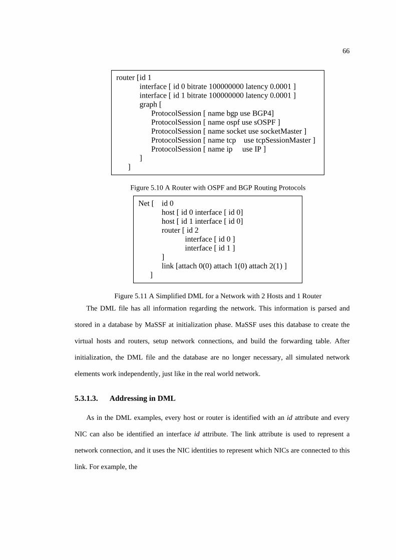
66
router [ id 1 interface [ id 0 bitrate 100000000 latency 0.0001 ] interface [ id 1 bitrate 100000000 latency 0.0001 ] graph [
ProtocolSession [ name bgp use BGP4] ProtocolSession [ name ospf use sOSPF ] ProtocolSession [ name socket use socketMaster ] ProtocolSession [ name tcp use tcpSessionMaster ] ProtocolSession [ name ip use IP ]
] ]
Figure 5.10 A Router with OSPF and BGP Routing Protocols
Net [ id 0 host [ id 0 interface [ id 0] host [ id 1 interface [ id 0]
router [ id 2 interface [ id 0 ] interface [ id 1 ] ] link [attach 0(0) attach 1(0) attach 2(1) ]
]
Figure 5.11 A Simplified DML for a Network with 2 Hosts and 1 Router
The DML file has all information regarding the network. This information is parsed and
stored in a database by MaSSF at initialization phase. MaSSF uses this database to create the
virtual hosts and routers, setup network connections, and build the forwarding table. After
initialization, the DML file and the database are no longer necessary, all simulated network
elements work independently, just like in the real world network.
5.3.1.3. Addressing in DML
As in the DML examples, every host or router is identified with an id attribute and every
NIC can also be identified an interface id attribute. The link attribute is used to represent a
network connection, and it uses the NIC identities to represent which NICs are connected to this
link. For example, the

67
link [ attach 0(0) attach 1(0) attach 2(1) ]
represents that there is a switch connecting host 0, host 1, and router 2, using interface 0, 0,
and 1 respectively.
The Net is also identified by the id. MaSSF supports hierarchical networks with nested Net
attributes. And each Net attribute can have multiple sub Net attributes, identified with different
id attributes. The Net, router, host, and interfaces defined in such a manner can be uniquely
addressed using the NHI scheme, where NHI represents the Network-Host-Interface. The
network address of Net attributes is formed by concatenating the id of the network definition at
each level starting from the DML root, separated by colons. Similarly, the NHI address of a host
or router is the encompassing Net addressing concatenated with the id of the host, separated by
colons. The NHI address of a NIC is the concatenation of Net and host address, followed by the
NIC id, enclosed in parentheses. For example, an NHI of 4:2:12(3) represents the third NIC of
host 12 in the network 4:2.
The NHI scheme can be used to globally address any host, router, or interface, uniquely.
However, when used in a DML file, the network address essentially starts from the root of the
DML Net; typically a local address is sufficient. For example, when we define a link in Net 4,
only the local address is used
Link [ attach 2:12(3) …]
In this way, a sub-network can be defined without knowing the upper-level network, and a
single definition can be used multiple times by different networks. This makes the DML quite
flexible when defining a hierarchical network.
NHI addressing is only used inside the DML file, and external users require IP addresses.
The user can specify an IP address for every NIC of the hosts and routers in the DML file or
MaSSF can automatically assign IP addresses according to CIDR address mechanism [60].

68
After assigning an IP address, the forwarding table will be setup automatically, according to the
configured routing protocols.
5.3.1.4. Routing in MaSSF
As in a real world router, packet forwarding in the MaSSF router is decided by a local
forwarding table, which is calculated by the routing protocols. We have implemented the OSPF
protocol for intra-domain routing and BGP4 protocol for inter-domain routing. As we already
see in the examples, these protocols can be installed in the router protocol stack.
Two versions of OSPF are implemented in MaSSF. The first is the static OSPF, which only
calculates the shortest-path routing of an AS at the beginning of simulation and it will not
respond to network changes during the simulation. However, it can still accept dynamic routing
information from BGP protocols. The second fully implements the specification of OSPFv2 [61]
and recalculates the routing table dynamically when experiencing router failure, link failure, or
heavy traffic congestion. Compared to the dynamic version, static OSPF is much simpler, and
requires less memory. Since all routers in an AS has the same view of the network, we can just
keep a single network database in an AS, and calculate forwarding tables for every router
together. The network topology database can be released after initialization. Dynamic OSPF, on
the other hand, has to keep the AS network topology information and calculate the forwarding
table by itself. In practice, we only use the static OSPF for large scale simulation, and use the
dynamic OSPF only when we really care about the routing dynamic inside an AS.
The BGP protocol in MaSSF is based on the SSF.OS.BGP4 model from SSFNet. The focus
of porting the BGP4 model from SSFNet to MaSSF, is not on to develop novel BGP simulation
technology, instead, the focus is to exploit the scalability offered by the MaSSF simulation
framework So, functionally the MaSSF implementation is fully compliant with the BGP-4
specification in the RFC1771[62], just like the original SSFNet BGP model. And it is also fully

69
validated with the test suits in SSFNet, covering functionality such as basic peering session
maintenance, route advertisement and withdrawal, route selection, route reflection, and internal
BGP.
One major consideration in our BGP implementation is the reduction of memory
consumption for better scalability. For a large network simulation, one big memory consumer is
the BGP routing table, since it grows exponentially with the number of ASes. To alleviate this
memory problem, we fully reuse routing entries among the three parts of BGP Routing
Information Base (RIB) [63]: Adj-RIBs-In, Loc-RIB, and Adj-RIBs-Out . Unlike the Java
automatic memory management of SSFNet, MaSSF manages all objects using reference
counters which reduce the memory consumption by 60%. The other big memory consumer is
the local forwarding table. In MaSSF, the BGP routers can work with OSPF routers insider an
AS and only broadcast default routing to external networks, instead of the whole routing table in
the BGP router. This is can greatly reduce the memory consumption and computation overhead
for a large AS with hundreds of internal routers. Of course the user can disable this feature if
they want to manually control the routing policy inside the AS.
5.3.2 Online Network Simulation
Online network simulation is to enhance traditional network simulation with supports for
direct execution of applications. Two major issues are discussed here, one is how to intercept
live application traffic and the other is how to inject the traffic to the traditional network
simulation.
5.3.2.1. Socket Level Interception
In order is to support direct execution of real applications in MaSSF, we need to intercept
live traffic from applications and present it to the network simulator. It can be achieved either at
the socket level by intercepting the send(), recv() network related system calls or at the IP

70
packet level by manipulating the IP packet directly. The difference between these two
approaches is whether or not the operating system’s TCP stack (see Figure 5.12) is used in the
data movement path. The advantage of the second approach is that it does not model the TCP
stack, leading to a much simpler implementation. However, using the original TCP stack
requires running the simulation in real time, since the OS TCP stack observes the real packet
RTT (round trip time) and adjusts its send rate according the RTT it observed. This is a big
constraint, since in many situations the physical resources are not fast enough to achieve real
time simulation. So MaSSF takes the first approach, intercepting the live traffic at socket level
for scaled-real time simulation.
Application2
send() recv()
Simulated Network
TCP Stack
TCP Stack
Application1
IP Packet IP Packet
Figure 5.12 Traffic Flow in a Real Operating System
As shown in Figure 5.13, MaSSF intercepts all network related system calls using a library
called WrapSocket, which can be either statically or dynamically linked to application programs.
Every virtual host has a corresponding Agent inside the simulator, and WrapSocket sends the
Agent a logical reference for each intercepted network operation. A detailed TCP stack is
implemented inside MaSSF and packet movement and timing are accurately simulated. Only
packet references are routed in the simulated network, while the real data stays in WrapSocket
and is delivered directly to the destination processes’ WrapSocket. There are no extra data
copies, and minimal real network traffic is incurred. When all required data arrive at the
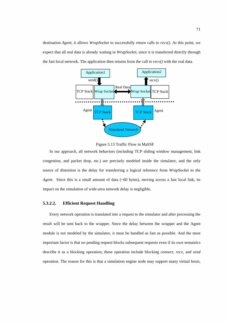
71
destination Agent, it allows WrapSocket to successfully return calls to recv(). At this point, we
expect that all real data is already waiting in WrapSocket, since it is transferred directly through
the fast local network. The application then returns from the call to recv() with the real data.
Application2 send() recv()
Real Data Wrap Socket
Wrap Socket
Agent Agent TCP Stack
TCP Stack
Simulated Network
TCP Stack
TCP Stack
Application1
Figure 5.13 Traffic Flow in MaSSF
In our approach, all network behaviors (including TCP sliding window management, link
congestion, and packet drop, etc.) are precisely modeled inside the simulator, and the only
source of distortion is the delay for transferring a logical reference from WrapSocket to the
Agent. Since this is a small amount of data (~60 bytes), moving across a fast local link, its
impact on the simulation of wide-area network delay is negligible.
5.3.2.2. Efficient Request Handling
Every network operation is translated into a request to the simulator and after processing the
result will be sent back to the wrapper. Since the delay between the wrapper and the Agent
module is not modeled by the simulator, it must be handled as fast as possible. And the most
important factor is that no pending request blocks subsequent requests even if its own semantics
describe it as a blocking operation; these operation include blocking connect, recv, and send
operation. The reason for this is that a simulation engine node may support many virtual hosts,

72
with many application processes connected to it. If the request handler blocks on one request, it
cannot handle requests from other processes or from other virtual machines.
Based on these considerations, the simulation module is implemented with the following
features.
1) Non-blocking Request Handling: All event handling must be non-blocking. For those
blocking operations, the block happens only in the wrapper; all operation within the simulator is
non-blocking. To achieve this, we exploit callback mechanisms in the simulator, implemented
through the Continuation construct.
Continuation {
int success();
int failure(int err_no);
};
For every blocking request, a continuation object is created and registered in the simulator.
For example, a blocking read operation can create and register a continuation on the
corresponding TCP session. When new data arrives, the simulator will check whether any
pending read continuation is registered and whether it is satisfied, if so, the success() function
will be called and the read result is sent back to the wrapper.
2) Event-based Request Dispatch: Every simulation node has a thread pool to accept
requests. Requests form the wrapper are first put into an event queue, and then handled by a
thread pool in FIFO model. The event handling is non-blocking, so only a small number of
threads are needed to handle a large number of clients (application processes).
3) Optimization for Select and Poll: All function calls are handled in a RPC-like approach,
except the select and poll calls. These calls are different. They have timeout mechanism with
the timeout values can be quite small and called very frequently. If they are implemented in a
straight forward fashion, that is, one request for per call and timeout in the simulator, the

73
overhead for some applications could be so large that it would affect the accuracy of the
simulation. Hence, these calls are handled separately. We do not send out a request for every
call, instead, we only send out a request when it is different from the last request, such as when
selecting on different socket sets. Timeouts only happen in the wrapper, and the simulator is not
involved. An old selection request will register a continuation, and it will either result in success
or be overwritten by a new selection on that socket. An invalid selection result must be sent
back to the wrapper when that selection has timeout. The wrapper can use sequence numbers to
distinguish invalid results.
Request Throughput
0
10000
20000
30000
40000
50000
60000
70000
1 2 4 6 8 10 20 40 60 80 100
120
140
160
180
200
Concurrent Clients
Thro
ughp
ut (r
eq/s
econ
d)
Figure 5.14 Request Throughput for a Single Simulation Engine
Figure 5.14 shows the request throughput of a single simulation engine node, versus
concurrent number of clients. For a single client, the throughput is about 2200 requests per
second, and the total throughput can reach 65K requests per second. This throughput seems
small, but it can support quite a fast network, since every request can correspond to a send
operation, which can be much larger than a network packet. Also, all simulation engine nodes
provide fully parallelized on requests handling, we can increase simulation engine nodes
numbers if necessary.
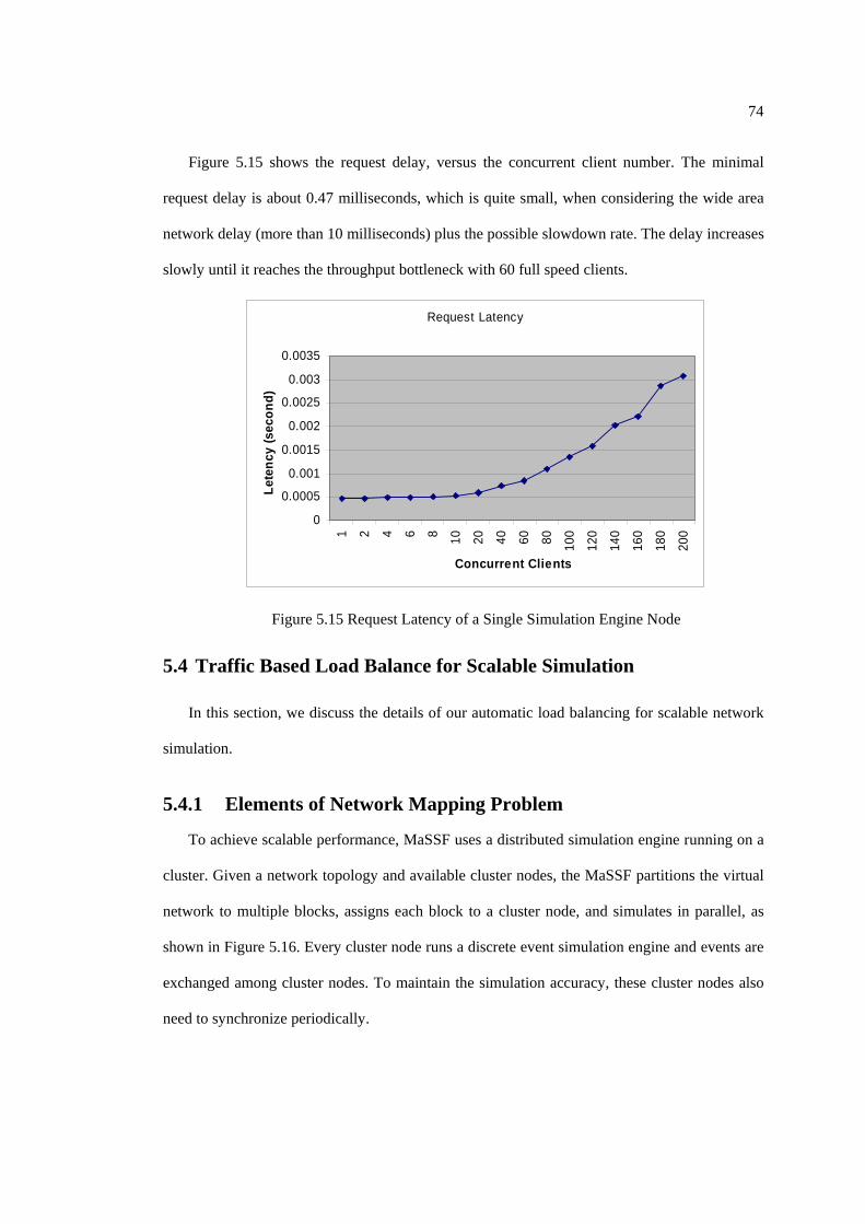
74
Figure 5.15 shows the request delay, versus the concurrent client number. The minimal
request delay is about 0.47 milliseconds, which is quite small, when considering the wide area
network delay (more than 10 milliseconds) plus the possible slowdown rate. The delay increases
slowly until it reaches the throughput bottleneck with 60 full speed clients.
Request Latency
0
0.0005
0.001
0.0015
0.002
0.0025
0.003
0.00351 2 4 6 8 10 20 40 60 80 100
120
140
160
180
200
Concurrent Clients
Lete
ncy
(sec
ond)
Figure 5.15 Request Latency of a Single Simulation Engine Node
5.4 Traffic Based Load Balance for Scalable Simulation
In this section, we discuss the details of our automatic load balancing for scalable network
simulation.
5.4.1 Elements of Network Mapping Problem
To achieve scalable performance, MaSSF uses a distributed simulation engine running on a
cluster. Given a network topology and available cluster nodes, the MaSSF partitions the virtual
network to multiple blocks, assigns each block to a cluster node, and simulates in parallel, as
shown in Figure 5.16. Every cluster node runs a discrete event simulation engine and events are
exchanged among cluster nodes. To maintain the simulation accuracy, these cluster nodes also
need to synchronize periodically.

75
Scalable Cluster System
Router
Host
Router
Router
Traffic Load
Figure 5.16 Mapping Routers to Physical Resources
For large simulations, the network mapping cannot be done manually or casually. Instead,
the mapping is a critical and demanding challenge, since we need to achieve load balance across
all cluster nodes. This is difficult because the workload on each physical node varies greatly,
depending both on the virtual mapping and network traffic in that subset of virtual network
(Figure 5.17). Furthermore, two more optimization goals should be considered. One is to
maximize link latency across partitions to reduce the frequency of synchronization among
simulation engines and maximize concurrency, a critical element of scalability for large scale
simulation. This feature is an attribute of our MaSSF system and all other network simulators
based on conservative discrete event simulation engines. The other optimization goal is to
minimize the communication of simulation events between simulation engine nodes. It is
expensive to transfer a simulation event across physical nodes both in terms of computation
overhead and communication latency. Also, the physical network of the simulation engine
nodes is often a performance bottleneck for the whole simulation. Hence, it is important to
minimize this communication.
The problem above is called the network mapping problem. To achieve the optimal load
balance even with known traffic is a NP-Hard problem[55]. However, in practice, a network
mapping problem can be naturally modeled as a graph partitioning problem and solved with the
classical graph partitioning algorithms.
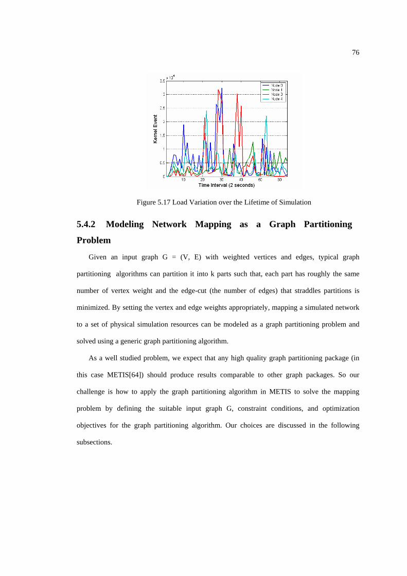
76
Figure 5.17 Load Variation over the Lifetime of Simulation
5.4.2 Modeling Network Mapping as a Graph Partitioning
Problem
Given an input graph G = (V, E) with weighted vertices and edges, typical graph
partitioning algorithms can partition it into k parts such that, each part has roughly the same
number of vertex weight and the edge-cut (the number of edges) that straddles partitions is
minimized. By setting the vertex and edge weights appropriately, mapping a simulated network
to a set of physical simulation resources can be modeled as a graph partitioning problem and
solved using a generic graph partitioning algorithm.
As a well studied problem, we expect that any high quality graph partitioning package (in
this case METIS[64]) should produce results comparable to other graph packages. So our
challenge is how to apply the graph partitioning algorithm in METIS to solve the mapping
problem by defining the suitable input graph G, constraint conditions, and optimization
objectives for the graph partitioning algorithm. Our choices are discussed in the following
subsections.

77
5.4.2.1. Input Graph
The input graph G is defined by two categories of parameters: network structure and traffic
information. The network structure includes detailed network topology, link latency, and link
bandwidth. In MaSSF, this information is stored in the network description file and can be
easily translated to a vertex and adjacent edge graph. Network traffic information is used to
define edge weights in the graph, and it may also affect vertex weights. In general, network
traffic information includes background traffic and foreground applications traffic, derived from
trace, model, or even live applications. How we approximate and model the expected traffic for
the simulation is the distinguishing key characteristic of our three different load balance
approaches. We will further focus on how to get that information in Section 5.4.3.
5.4.2.2. Constraints
In a graph partitioning problem, the constraint is the vertex weight to be balanced among
multiple vertices. In the network mapping problem, the vertex weight can be defined as
weighted sum of computation and memory requirement on each simulation engine node. In the
MaSSF implementation, the computation requirement mainly comes from the logic for packet
processing, which depends on network connection, routes, and traffic intensity. It is calculated
based on the maximal bipartition flow of all traffic flowing through a network node. The
memory requirement is mainly based on the routing table size. The routing table size is in the
order of O(n2), where n is the number of routers in an AS (Autonomous System). We also use
multiple constraints to balance different kinds of vertex weights together.
5.4.2.3. Objectives
In a graph partitioning problem, the objective is the edge-cut to be minimized. In the
network mapping problem, the optimization can use two objectives, which means two different

78
ways to weight the edges. The first one is to maximize link latency across partitions. This can
reduce the frequency of synchronization among simulation engines and maximize concurrency
in the simulation, which is very important for scalability for large scale simulation. This feature
is an attribute of our MaSSF system and all other network simulators based on conservative
discrete event simulation engines.
The second objective is to minimize the communication of simulation events across
simulation engine nodes, since it is expensive to transfer a simulation event across physical
nodes both in terms of computation overhead and communication latency. Also, the physical
network of the simulation engine nodes is often a performance bottleneck for the whole
simulation; hence, it is important to minimize this communication. With detailed traffic
information, we can estimate the number of simulation events on each single link and use it to
calculate the edge weight. How to get such traffic information is the major topic of Section
5.4.3.
5.4.2.4. Multi-Objective Graph Partitioning
In last subsection, two objectives are described. Both of them are important and sometimes
in opposition.
1) Apply the single objective algorithm for maximal link latency across partitions,
get the optimization edge-cut Clatency.
2) Apply the single objective algorithm for minimal network traffic across
partitions, get the optimization edge-cut Cbandwidth.
3) Assign each edge weight to
bandwidth
bandwidth
latency
latency
Cw
Cw
conbined ppw )1( −+=
where p is the user controllable weight of the latency objective.
4) Apply the single objective algorithm with the new normalized edge weights.
Figure 5.18 The Multi-Objective Graph Partitioning Algorithm

79
The challenge is to figure out how to set edge weights to represent the requirement of both
objectives, and still provide the user predictable control on tradeoff. A simple combination-
based approach (e.g. simply add two weights to a single weight) does not make sense.
Applying the algorithm presented in [42], we can combine two dissimilar weights in a
predictable way and use the available single objective METIS partitioning package. This
algorithm is based on the intuitive notion of what constitutes a good multi-objective partition.
That is, a good solution should be close to the optimization solution for each single objective.
Applying this approach on our network mapping problem, we get the algorithm in Figure 5.18:
Network Structure
Partitioned Network
Traffic Information
Graph Preparation
G Constraints Objectives
Graph Partitioning Algorithms
Figure 5.19 Process of Network Mapping
In summary, the mapping process can be modeled as shown in Figure 5.19. First, it takes
the network structure and traffic information as input, creates a graph G, and builds objectives
and constraints of graph partitioning algorithms. Then it applies partitioning algorithms to get
the partitioned network. The partitioned network incapacitates the mapping of emulated
network nodes to physical resources. We may have different abstraction of network mapping
problems and use different constraints and objectives in the graph partitioning algorithm;
however, we believe what we present above is straightforward and should have reasonable

80
results with small overhead. The problem left is how to collect and use the traffic information,
which will be discussed in the following section.
5.4.3 Traffic Based Network Mapping
Three different approaches are explored for network mapping. These approaches vary in
how network topology, background traffic, and application traffic are represented and used in
the partition. The ability to predict the simulation workload (i.e. network traffic) accurately
enables better partitioning and therefore better load balance. However, there are tradeoffs
between the specificity of the information used and the generality of the partition produced.
5.4.3.1. Network Topology-Based Mapping (TOP)
Our first approach only considers the simulated network topology, link bandwidth, and
latency, in which each virtual node is weighted with the total bandwidth in and out of it. The
optimization objective is to maximize the link latency between simulation engine nodes, as
discussed in Section 5.4.1. This maximizes decoupling, supporting efficient parallel simulation.
This basic approach is simple and fast, and represented the state of art as we began.
Therefore, it forms a performance baseline for our experiments. It should work well for well-
engineered networks with evenly distributed traffic. In such networks, the link bandwidth
usually determines the routes that are placed over the links, and since networks are typically
engineered to match the demand, link bandwidth is closely related to real traffic. For example,
this model is expected to be effective when we want to study the web traffic on Internet, which
is composed of lots of small web browsing flows.
5.4.3.2. Application Placement-Based Mapping (PLACE)
With precise traffic information, we can do a better mapping. The second approach is based
on the observation that simulated network traffic typically consists of a background and a

81
foreground load. Foreground traffic is created by the target application that the user wants to
study, and background traffic is used to provide realistic network conditions. Both traffic loads
are estimated separately, and then combined to predicate the aggregated traffic data for better
network mapping. We call this approach PLACE.
The background traffic is generated using simple traffic models based on the network
topology, and can be explicitly controlled by the user of the network simulator. In this case, it
is reasonable that all traffic generators can provide some prediction of their generated traffic
load, for example, specifying the average traffic bandwidth between two endpoints. Because the
background traffic represents an aggregate of traffic, such a gross characterization can be
reasonably accurate.
Due to the nature of configuring application, the foreground load is typically the live traffic
from a small set of application programs. Unlike background traffic prediction, it is difficult for
users to predict the traffic of the real application. First, the live traffic has complex dynamic
behavior that is hard to model (that is why we need a network emulator to study it). Second,
users may not have the required knowledge to describe this information (lacking either
application knowledge or the computer systems knowledge). As an approximation, we
determine the traffic injection points of the application, where its processes attach to the
simulated network, assuming that the application fully utilizes the network link at each injection
point and every node talks to all other nodes with evenly distributed bandwidth. While this
approximation may seem coarse at first glance, it is acceptable when considering that most
target applications in simulation are complex and network intensive.
With the source/destination pairs of all traffic flows, the aggregated traffic on each link can
be computed by summing the contribution from each flow. To identify the routes used in the
simulated network, we instantiate the simulated network and detect the actual routes used
(based on dynamically generated routing tables and routing protocols). To get the routing

82
information, we implement the ICMP protocol inside MaSSF, and use the real Linux traceroute
tool to discovery the routing paths between each source-destination pair. To reduce the number
of traceroute execution required, we could use one representative endpoint for each sub-
network and only discover the route paths between those sub-network representatives.
With this predicted traffic information, the approach in Section 5.4.3.1 can be improved by
recalculating vertex/edge weights. This extra information also enables another objective, which
is to minimize the traffic across partitions. In the approach, the multi-objective graph
partitioning algorithm described in Section 5.4.2.4 is used.
5.4.3.3. Profile-Based Mapping (PROFILE)
The third approach uses profiling techniques to obtain traffic information automatically
from simulation experiments. The profiles are then used to estimate future network use, and to
improve the network mapping. Typically this involves an initial simulation experiment using an
initial partition and traffic monitoring. The simulation yields detailed traffic information and the
network can be repartitioned based on this information.
The critical challenge for this approach is the efficient collection and representation of
traffic information during profiling, and the use of this information to repartition the network. In
MaSSF, we implement the Cisco NetFlow-like [65] function on each simulated router. This
functionality is used to record every traffic flow on each router to a local file. The dump files
record the average bandwidth and duration of every flow on every router. Parsing the dump files
allows computation of the aggregated traffic on every router and link in the network. By tuning
the granularity of the NetFlow, we can get detailed network traffic information with small
overhead.
In our implementation, the real network traffic data does not actually travel through the
simulator; only packet references are processed by it. Instead of using the real network

83
bandwidth (MB/s) as the bandwidth measurement, the number of packets in a flow is used,
since the real load in the simulator depends on the number of packets it processes. The live
traffic injection overhead is also measured by the number of requests coming from the
application.
With much more accurate traffic information about the virtual network from the profile data,
the same multi-objective graph partitioning algorithm described in Section 5.3.2.4 is applied to
get better load balance.
5.4.3.4. Preliminary Results
We implemented these three partition algorithms in the MaSSF and applied them to the
network simulations, with different network topologies and different applications. The network
topologies are in range of 60-300 hosts and routers, simulated with less than 10 physical nodes
(Table 5.1). These studies show that exploiting static topology and application placement
information can achieve reasonable load balance, but a profile-based approach further improves
load balance for even large scale network simulation. In our experiments, PROFILE improves
load balance by 50% to 66% and simulation time is reduced up to 50% compared to purely
static topology-based approaches. More details are reported in [66].
Table 5.1 Network Topology Setup in Premier Study
Network
Topology Router Host
Simulation
Engine Node
Campus 20 40 3
TeraGrid 27 150 5
Brite 160 132 8

84
5.4.4 Hierarchical Load Balance Approach
5.4.4.1. The Small Achieved MLL Problem
When we apply the TOP and PROF approaches to larger networks (e.g. 10,000 routers
running on 100 nodes), neither of them gets satisfactory results. Checking the partition output
manually reveals that the common reason for poor performance is that the achieved Minimal
Link Latency (MLL) across partitions is insignificant when compared to the synchronization
cost. This produces an overall simulation efficiency that is quite low. For example, for one
network of 10,000 routers, the achieved MLL was only 0.1ms; far less than the synchronization
cost of ~0.58ms for 100 simulation engine nodes (see Figure 5.20). Synchronization cost is the
time used by the simulation engine nodes for global synchronization, which need to be executed
every MLL time. In such a situation, the majority of the time will be spent in synchronization –
even perfect load balance would only moderate efficiency. This situation is quite different from
the 1ms MLL for a 160 router network and 0.9ms synchronization cost for 8 simulation engine
nodes in our previous experiments[66].
Synchronization Cost of TeraGrid Cluster
0100200300400500600700800900
2 6 16 48 80 112
Node Number
Del
ay(m
icro
seco
nd)
Figure 5.20 Synchronization Cost of the TeraGrid NCSA Cluster

85
5.4.4.2. Understanding Achieved MLL
The example above exposes a major problem with the existing load balance approaches. In
TOP and PROF mappings, the link latency is converted to edge weight of the graph G, and
smaller link latency leads to a larger edge weight. When the graph partitioner archives minimal
edge-cut across partitions, it is less likely to partition across the link with small link latency,
since it corresponds to a large edge weight. However, the optimization goal is the not the MLL,
but the minimum edge-cut (the sum of all edge weights that cross partitions). When we have a
large graph, the partitioner becomes less sensitive to the MLL, since even the large edge weight
from a link with MLL may only be a small part of the final edge-cut.
We may tune the converting algorithm to make the edge weights of small link latencies
large enough that it is unlikely they will across partitions, but this depends highly on the
network topology, number of the simulation engine nodes, and the physical synchronization
cost.
5.4.4.3. Optimizing MLL
To address the issue of small achieved MLL, a new hierarchical partition algorithm is
designed. To avoid partitioning across edges with small link latencies, edges with latencies
smaller than a threshold, LL, are removed from the input graph (by merging nodes) to the
partitioner and are added back to the partitioned output later. In this way, we can guarantee the
worst-case of MLL. However, this produces a new problem —how do we choose the latency
threshold, LL. If the threshold is too large, it will damage load balance, while if it is too small it
will achieve a smaller MLL than possible. Instead of guessing the threshold, our approach is to
simply try all reasonable thresholds, create a partition for each, evaluate these partitions, and
then pick up the best partition. This is feasible because the partition can be done fast, even for

86
large networks, and different partition outputs can be evaluated without running the simulation.
The pseudo code for hierarchical partitioning is present in Figure 5.21.
Input: graph G, partition N, and synchronization cost C
Output: the best partition P of graph G
Hierarchical Partition:
Set the initial Threshold of MLL (Tmll)
Loop through all reasonable Tmll:
Get the dumped graph Gd(Tmll)
Partition the Gd(Tmll) using an existing partitioner, and get P(Tmll)
Evaluate the partition result Pd(Tmll)
Pickup the best partition Pd(Tmll)
Get the best partition P of original G
Figure 5.21 Hierarchical Graph Partitioning Algorithm
This algorithm requires the graph, G, the partition number, N, and the synchronization cost
of the simulation engine nodes, C. Figure 5.20 shows the synchronization cost of the TeraGrid
SDSC cluster, which is used for all simulations in this paper. We use the synchronization cost
to set the initial threshold of MLL (Tmll) based on knowledge of the desired number of
simulation engines. A Tmll is required to be larger than the synchronization cost; otherwise all
time will be spent on synchronization, giving poor efficiency. Given the Tmll, the original graph
G is reduced to a dumped graph Gd by collapsing nodes with link latency less then Tmll into a
single node. Then any existing partition can be applied to the dumped graph Gd and get the
partitioner output. By increasing the Tmll step by step (0.1ms in our experiments), we can get a
sequence of partitions, and the remaining question is how to select amongst them.
To evaluate the candidate partitions, we use an efficiency metric Efficiency (E), which
consists of two factors, Es and Ec. The first factor (Es) represents the efficiency decided by the
achieved MLL and is calculated:
Es = (MLL – CN)/MLL,

87
where CN is the synchronization cost of N simulation engine nodes. The latter (Ec)
represents the result of computational load balance and is calculated by:
Ec = Caverage/Cmax,
where Caverage is the estimated average load (simulation event rate) on all nodes, and Cmax is
the max load of all nodes. The final efficiency E is Es * Ec, where larger values of E correspond
to better partitions. Maximizing Es and Ec separately does not work because they represent the
tradeoff between simulation efficiency and available parallelism. Larger Es means better
simulation efficiency, but it also means less parallelism available, since smaller MLL leads to a
more coarse-grained partition graph.
In summary, our hierarchical partitioning approach balances the parallelism and decoupling
concerns in generating a good network partition. To do so, it generates and evaluates many
possible partitions. Because we can create graph partitions and evaluate graph partitions quickly,
the METIS graph partitioner[64] used in MaSSF can partition a graph with 10,000 vertexes in
about 10 seconds, we can consider thousands of possible Tmll.
5.5 Summary
In this chapter, we presented the system design and implementation of the MicroGrid
toolkit. We first introduced the soft real-time process scheduler for computation resource
simulation, and then the scaled real-time online network simulator MaSSF. These two
components together can provide accurate and efficient virtual grid modeling. After that, we
introduced the traffic based load balance algorithms to improve the scalability of the network
simulator, which is critical to support large scale virtual grid simulation.

88
Chapter 6 Validation
So far, we have presented our approaches and system design for accurate large-scale virtual
grid modeling. However, a design with these approaches and techniques alone is insufficient to
enable the systematic study of dynamic behavior. As any simulation tools, before it can be used
in any real research studies, it must be validated that the simulation results are accurate
comparing the real system behaviors; otherwise, it is useless. In this chapter, we provide
validation of the constituent models and the entire MicroGrid system on applications.
6.1 Methodology and Experimental Environment
To validate the MicroGrid system design and implementation, we first provide validation of
constituent models, including validation of the CPU resource model on one and several virtual
resources per physical resource and validation of the online network simulation models
exercised by real transport protocol stacks. Based on validation of different simulation models,
we provide validation of the whole MicroGrid system on a range of grid application programs
ranging from kernels to full-blown applications on two grid resource configurations.
The basic methodology for validation is to run applications, either real applications or
benchmarks written by ourselves, on physical resources and collect the performance data, such
as the execution time. Then we use the MicroGrid to simulate the physical resources and
execute the same applications on simulated environments. Thanks to the capability of direct
application execution on MicroGrid, the simulated application performance results are directly
comparable to what we get from the execution on physical resources.
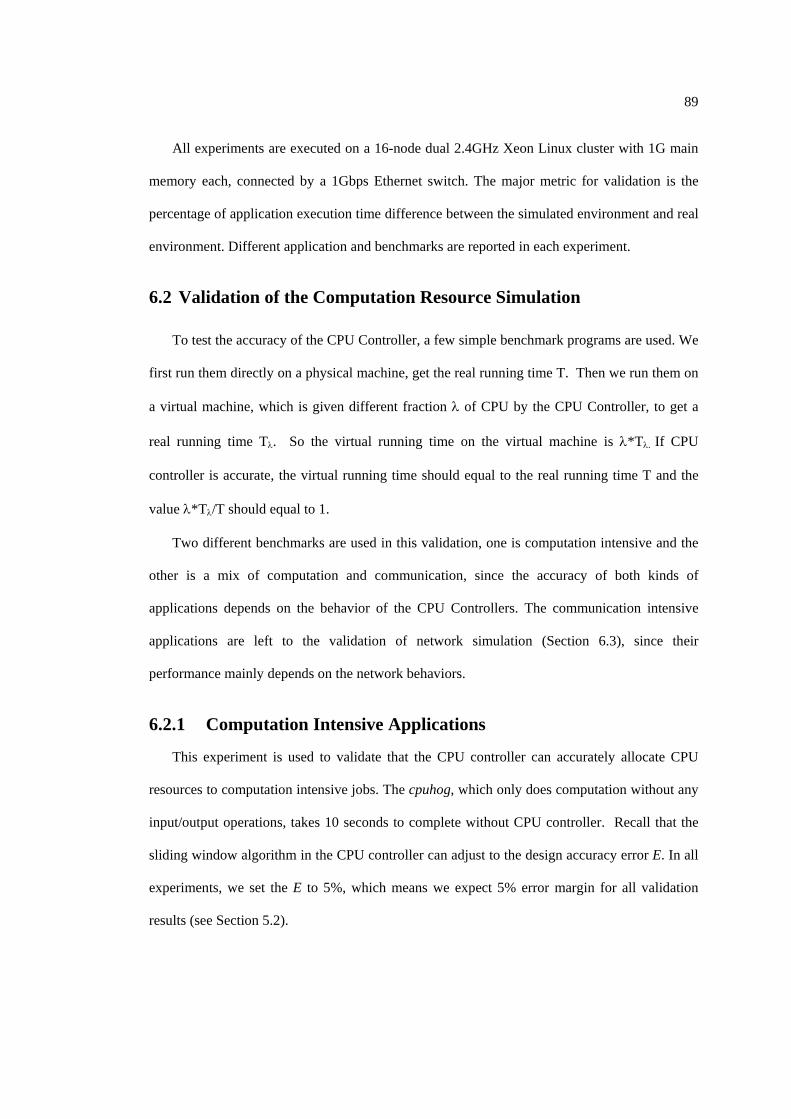
89
All experiments are executed on a 16-node dual 2.4GHz Xeon Linux cluster with 1G main
memory each, connected by a 1Gbps Ethernet switch. The major metric for validation is the
percentage of application execution time difference between the simulated environment and real
environment. Different application and benchmarks are reported in each experiment.
6.2 Validation of the Computation Resource Simulation
To test the accuracy of the CPU Controller, a few simple benchmark programs are used. We
first run them directly on a physical machine, get the real running time T. Then we run them on
a virtual machine, which is given different fraction λ of CPU by the CPU Controller, to get a
real running time Tλ. So the virtual running time on the virtual machine is λ*Tλ. If CPU
controller is accurate, the virtual running time should equal to the real running time T and the
value λ*Tλ/T should equal to 1.
Two different benchmarks are used in this validation, one is computation intensive and the
other is a mix of computation and communication, since the accuracy of both kinds of
applications depends on the behavior of the CPU Controllers. The communication intensive
applications are left to the validation of network simulation (Section 6.3), since their
performance mainly depends on the network behaviors.
6.2.1 Computation Intensive Applications
This experiment is used to validate that the CPU controller can accurately allocate CPU
resources to computation intensive jobs. The cpuhog, which only does computation without any
input/output operations, takes 10 seconds to complete without CPU controller. Recall that the
sliding window algorithm in the CPU controller can adjust to the design accuracy error E. In all
experiments, we set the E to 5%, which means we expect 5% error margin for all validation
results (see Section 5.2).

90
Figure 6.1 The cpuhog for Single Virtual Resource
Figure 6.1 are the results for single virtual resource, which show that when there is only
one process, the error is almost always in 2%, except when it is near full utilization of the
underlying physical resource. At 90% CPU, we observe a 6.7% error. When there are multiple
processes, the running time becomes about 6-8% longer.
To understand the performance of CPU controller with multiple virtual resources on a
single physical machine, two groups of experiments are executed with three virtual resources
and five virtual resources on a physical machine respectively. Each time, the virtual resources
are created, and one cpuhog is launched on each virtual resource. Then the average completion
time is used as the virtual running time to calculate the efficiency rate λ*Tλ/T. The results are
shown in Figure 6.2. The “aggregated CPU speed” is the sum of speeds of all the virtual
machines. Most of the tests have an error of less than 4%, with the one exception of a 9% error
when total CPU is 78%.

91
Figure 6.2 The cpuhog for Multiple Virtual Resources
The inaccuracy for 90% CPU in Figure 6.1 and for 78% CPU in Figure 6.2 comes mainly
from the 5% design accuracy error in the sliding window algorithm: Since we allow 5% error
and we always choose the window size as small as possible, when the virtual machine speed is
90%, we would schedule the application for six of seven jiffies rather than nine of ten, which
causes a equivalent speed of 85.7% CPU with 4.8% error from 90% CPU; in the multiple-
virtual resource experiments, each virtual machines has 26% CPU and is scheduled for one jiffy
every four jiffies, which leads to 25% actually speed with about 4% error for 26% CPU.
These experiments show that the CPU controllers can efficiently simulate multiple virtual
resources on a single physical resource and still provide accurate computation resource
modeling for computation intensive applications.
6.2.2 Applications with Mixed Computation and Communication
This experiment is designed to demonstrate that the CPU controller can achieve accurate
performance for application with mixed computation and communication. As discussed in
Section 5.2, these applications represent much larger challenge than computation intensive
applications, because the CPU controller has no idea whether a waiting process is waiting for

92
network delay or is just scheduled out by the operating system. The mixhog executes
computation and communication combination in loop. We can control the length and ratio of
computation and communication to check how the CPU controller behaves for different
application patterns. The CPU controller design still uses a 5% design accuracy error (see
Section 5.2).
Figure 6.3 shows the accuracy of the CPU controller under different communication
granularity. The communication and computation ratio in the mixhog is fixed (1:1, 1:2, and 1:3)
and the communication time (network delay) changes from 10ms to 100ms in these experiments.
The errors are always within 10%, except when the communication delay is so small that it is
comparable to the OS scheduling granularity (10ms).
CPU Control of different Granuarity
0
0.2
0.4
0.6
0.8
1
1.2
10 9 8 7 6 5 4 3 2 1
network delay (10ms)
effic
ienc
y ra
te
1:011:021:03
Figure 6.3 The mixhog with Different Communication Granularity
Figure 6.4 and Figure 6.5 are the results of CPU controller accuracy against different virtual
CPU speed. We can see that the accuracy changes according to the virtual CPU speed, due to
the fact that the sliding window size. As we have discussed in Section 5.2, larger sliding
window size can lead to larger error. When most time the error is less than 10%, the error can
reach 20% when the virtual CPU speed is at 30%, 40% and 60%.

93
CPU control with 20ms network delay
0
0.2
0.4
0.6
0.8
1
1.2
10%
20%
30%
40%
50%
60%
70%
80%
90%
100%
expected cpu speed
effic
ienc
y ra
te
ratio(1/2)ratio(1/3)
Figure 6.4 The mixhog with 20ms Network Delay
CPU control with 30ms network delay
0
0.2
0.4
0.6
0.8
1
1.2
10%
20%
30%
40%
50%
60%
70%
80%
90%
100%
expected cpu speed
effic
ienc
y ra
te
ratio(1/2)ratio(1/3)
Figure 6.5 The mixhog with 30ms Network Delay
In summary, our experiments show that the CPU controller can model CPU speed
accurately. The multiple virtual resources experiments also demonstrate its capability to model
multiple virtual CPUs on one physical machine accurately.
6.3 Validation of Network Simulation
To test the accuracy of the network simulation, the main focus is on checking the
correctness of simple TCP application, since this simple test involves the most important and
complex part of the network simulation, the TCP protocol implementation. A majority of

94
network application performance depends on the TCP protocol behaviors. This simple test can
also validate if the CPU controller can guarantee quick response time (Section 5.2), and if the
traffic interception and requests handling is quick enough with negligible overhead (Section
5.3).
We use a client/server program tcpSender/tcpRecver which sends and receives packets
using TCP/IP between two nodes. In each iteration, the sender sends a message to the receiver
then wait for a one-byte reply from the receiver. The tcpSender can report the latency for each
message and the achieved network throughput, under different message sizes. We want to
compare results from simulated networks to those from real networks. If no real data available,
we use the theoretical values as metrics.
When message size is small, the latency for each iteration is close to the half of network
round trip time (RTT); when message size is large enough, the throughput approximates the
maximum bandwidth between the two nodes. The TCP throughput is affected by network
latency (L), TCP window size (W), network capacity (C), and packet loss[67]. If there is no
packet loss, the maximum throughput should be close to:
Throughput = min(C, W/(2*L))
6.3.1 Validation of Local Area Network
Our experiments first test the real network performance between two nodes on a cluster.
The nodes are dual Xeon 2.4GHz machines connected by GigE, configured with 128KB TCP
window. Experiments show that real network has latency 0.222ms and bandwidth 782.87Mbps.
On the MicroGrid, we simulate the two nodes with 128K TCP window and 0.2ms wire latency.
The simulated results of different virtual CPU speeds are shown in Figure 6.6 and Figure 6.7.

95
Figure 6.6 Network Throughput on GigE LAN
Figure 6.7 Network Latency on GigE LAN
The figures show that the virtual bandwidth (simulated) is close to the target bandwidth
when virtual CPU speed is faster than 25% of 2.4GHz Xeon. When virtual CPU speed is not
fast enough to support the memory and I/O operations, the bandwidth falls off.
The network latency is about 0.15ms longer than the configured wire latency. This is
presumed to be due to Agent overhead, overhead through TCP/IP stacks, and the overhead of
the MaSSF simulator.

96
6.3.2 Validation of Metro Area Network
The next set of tests use a network topology with a 1ms latency between the two nodes, and
varies the TCP window size from 32KB to 128KB. The results of different CPU speeds are
shown in Figure 6.8 and Figure 6.9.
Figure 6.8 Network Throughput on MAN
Figure 6.9 Network Latency on MAN

97
In this case, the network capacity is not the bottleneck any more, so the TCP throughput is
mainly decided by latency and TCP window size. We calculate the throughput upper bound in
theory, as shown in Table 6.1.
From Figure 6.8 and Table 6.1 we see that our simulator achieves 82-90% of the theoretical
maximum bandwidth. Considering the overheads on TCP stacks and application’s memory
operations, these are excellent results.
As for latency, the simulated value, as shown in Figure 6.9, is about 0.25ms higher than the
configured wire latency. Still, this is due to overheads on TCP stacks, application memory
operations, and MaSSF overhead.
Table 6.1 Theoretical Maximum Throughput on a Network Channel
32KB 48KB 64KB 128KB
1 ms 128Mbps 192Mbps 256Mbps 512Mbps
5ms 25.6Mbps 38.4Mbps 51.2Mbps 102.4Mbps
10ms 12.8Mbps 19.2Mbps 25.6Mbps 51.2Mbps
6.3.3 Validation of Wide Area Network
The following figures in Figure 6.10 show the bandwidth on network channel with latency 5
ms and 10ms respectively. The results are consistent with the theoretical bounds in Table 6.1.
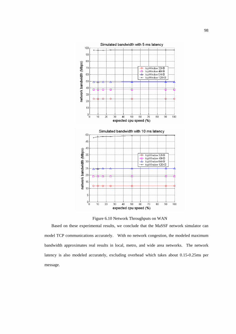
98
Figure 6.10 Network Throughputs on WAN
Based on these experimental results, we conclude that the MaSSF network simulator can
model TCP communications accurately. With no network congestion, the modeled maximum
bandwidth approximates real results in local, metro, and wide area networks. The network
latency is also modeled accurately, excluding overhead which takes about 0.15-0.25ms per
message.

99
We did not evaluate the simulator with network congestion, although our simulator supports
the capability to model competitive traffic (background traffic). Performance with congestion is
not easy to evaluate since it depends on the competitive traffic model. Here we also provide no
validation on routing protocols such as OSPF and BGP4, instead, there are validation test suites
coming with the software package.
6.4 Validation of the MicroGrid on Applications
We have provided validation on each individual simulation module. But this is not enough,
since what we really care is if these simulation modules together can provide accurate modeling
of a virtual grid environment. More specifically, does the scaled real-time mechanism
effectively coordinate multiple resources simulation modules and create correct simulation
results? Can the CPU controller handle mix computation and communication well for real
applications? To answer these questions, the best approach is to validate the MicroGrid on real
applications which can exercise most components together with large traffic and computation
loads.
6.4.1 Applications
In this section, we run five classic applications on both real environment and virtual
environment simulated using the MicroGrid. Before the results, we first introduce the five
applications briefly. These applications are used in the GrADS project[9].
All five applications are SPMD MPI applications and have been previously tested on the
GrADS testbed in various real-world experiments. These applications were integrated into the
GrADS framework and tested in various experiments as part of the following efforts:
ScaLAPACK [68], Jacobi [69], Game of Life [69], Fish [70], and FASTA [71].
ScaLAPACK is a popular software package for parallel linear algebra, including the
solution of linear systems based on LU and QR factorizations. We use the ScaLAPACK right-

100
looking LU factorization code based on 1-D block cyclic data distribution. The application is
implemented in Fortran with a C wrapper. The data-dependent and iteration-dependent
computation and communication requirements of ScaLAPACK provide an important test for the
MicroGrid simulation. In our experiments we used a matrix size of 6000x6000.
FASTA The search for similarity between protein or nucleic acid sequences is an important
and common operation in bio-informatics. Sequence databases have grown immensely and
continue to grow at a very fast rate; due to the magnitude of the problems, sequence comparison
approaches must be optimized. FASTA is a sequence alignment technique that uses heuristics to
provide faster search times than more exact approaches, which are based on dynamic
programming techniques. Given the size of the databases, it is often undesirable to transport and
replicate all databases at all compute sites in a distributed grid. We use an implementation of
FASTA that uses remote, distributed databases that are partially replicated on some of the grid
nodes. FASTA is structured as a master-worker and is implemented in C. For MicroGrid
validation purposes, an important aspect of FASTA is that each processor is assigned a different
database (or portion of a database) so the MicroGrid must properly handle input files and
provide proper ordering of data assignments onto processors. In our experiments the sizes of the
databases are 8.5MB, 1.7MB and 0.8MB respectively. The query sequence is 44KB.
The Jacobi method is a simple linear system solver. A portion of the unknown vector x is
assigned to each processor. During each iteration, every processor computes new results for its
portion of x and then broadcasts its updated portion of x to every other processor. Jacobi is a
memory-intensive application with a communication phase involving lots of small messages. In
our experiments we used a matrix size of 9600x9600.
The Fish application models the behavior and interactions of fish and is indicative of many
particle physics applications. The application calculates Van der Waals forces between particles
in a two-dimensional field. Each computing process is responsible for a number of particles that

101
move about the field. The amount of computation depends on the location and proximity of
particles, so Fish exhibits a dynamic amount of work per processor. In our experiments we used
6,000 particles.
Conway’s Game of Life is a well-known binary cellular automaton. A two-dimensional
mesh of pixels is used to represent an environment of cells. In each iteration every cell is
updated with a 9-point stencil and then processors send data from their edges (ghost cells) to
their neighbors in the mesh. Game of Life has significant memory requirements compared to its
computation and communication needs. In our experiments we used a matrix size of 9600x9600.
6.4.2 Experiment Environment
We use a subset of the multi-site testbed for the GrADS project as our testbed. The 11
machines used are as following:
UCSD cluster: four 2100+ XP Athlon AMD (1.73 GHz) with 512 MB RAM each. These
systems run Debian Linux 3.0 and are connected by Fast Ethernet.
UIUC cluster: three 450 MHz PII machines with 256MB memory connected via TCP/IP
over 1Gbps Myrinet LAN. These systems run RedHat Linux 7.2.
UTK cluster: four PIII 550 MHz machines with 512MB memory, running RedHat Linux
7.2, and connected with Fast Ethernet.
The three sites are connected by the Internet2 network with 2.4Gbps backbone links. During
our experiments, we observed NWS latency and bandwidth values over a period of 12 hours and
obtained ranges as shown in Table 6.2.
In our simulation, we configure all the machines to have 64KB TCP window. The wide
area latency is as shown in Table 6.2; the LAN latency is 0.2 ms. We have to remind the
audience that, the simulated LAN latency might higher than real latency due to simulation

102
overhead as shown in Section 6.3; while the simulated WAN bandwidth will higher than real
bandwidth due to lack of contention.
Table 6.2 Network performance of the testbed, reported by NWS
UCSD machine UIUC machine UTK machine
UCSD machine 60-80Mbps,
0.2 ms
3-7Mbps
31 ms
4-6Mbps
30 ms
UIUC machine 3-7Mbps
31 ms
115-220Mbps
0.2 ms
7-17Mbps
11 ms
UTK machine 7-8Mbps
30 ms
12-18Mbps
11 ms
82-87Mbps
0.2ms
6.4.3 Simulation Results
Two groups of experiments are conducted on those sites: “Cluster” group uses four UTK
machines to do clustering computation; “Grid” group uses three machines from each of the
three sites. Both groups use a separate UCSD machine to run Globus gatekeeper. The results
are shown in Figure 6.11.
103
Figure 6.11 Running Time of Applications
For the cluster, all applications run slower on the MicroGrid than on real testbed; most of
them have error in 6%-27%, except 66% for ScaLAPACK. The extra overhead comes from
two major sources: 1) The MaSSF has some overhead which increases network latency. 2)
WrapSocket wraps many system functions for simulation, which will cause some overhead.
For the grid environment, the simulated time has about 5% - 35% errors. We can see
several interesting differences from the cluster results. ScaLAPACK still runs slower on the
MicroGrid than on real testbed, but much closer than on cluster, because ScaLAPACK uses a
lot of small communications and the simulation overhead will have more impact on simulated
LAN latency than on simulated WAN latency (as shown in Section 6.3). Fish and GameOfLife
run faster on the MicroGrid than on real grid. A possible reason is that they both use many
large communications, and the simulated network bandwidth is higher than real system due to
lack of contention.
6.5 Summary
In this chapter we provide the validation on the MicroGrid system and therefore on our
approaches for virtual grid modeling. Specifically, we provide:

104
1)Validation of computation resource simulation. Experiments with the MicroGrid on
simulating multiple virtual resources per physical resource match closely within 2%-9%, even
for applications with mix of computation and communication.
2)Validation of the online network simulation. Latency results reported by the TCP
client/server benchmark vary only 0.15-0.22ms for different networks, and the throughput
results vary from 5% to 18%.
3)Validation of the whole MicroGrid system on a range of grid application programs on
two grid resource configurations. Most application execution times match within 65% to 95%.
With a solid validation of the MicroGrid toolkit, a range of interesting experiments for grid
applications and middleware is virtually unbounded.

105
Chapter 7 Scalability Studies
In this chapter two large network simulations, one single AS network of 20,000 routers and
one multi-AS network of 100 ASes with 200 routers each, are used to demonstrate the
scalability of the MicroGrid system. This scale of network is quite large, even comparing to the
largest real grid project testbeds. For example, the Grid2003 [3] has 27 sites across US and
Korea which collectively provides more than 2000 CPUs. At the same time, hierarchical traffic-
based partitioning and mapping approaches in Section 5.4 are used in these experiments to show
the scalability improvement. Practically, now it is possible to do realistic full grid simulation
with the MicroGrid in a cluster.
7.1 Experimental Setup
7.1.1 Improve Scalability through Load Balance
The MicroGrid must be scalable to support the study of large networks, resources,
middleware, and applications. While most resources can be naturally simulated in parallel with
enough physical resources, all the coordination, synchronization and dynamic interaction
amongst resources must go through network communication. This means the network must be
simulated as a single system with global coordination, and thus the scalability of network
simulation is a critical challenge for the entire MicroGrid system. In particular, the challenge is
scalable detailed packet-level simulation combined with online simulation. We require packet-
level simulation to ensure fidelity in simulation of network, protocol, and application behavior.
Higher level simulation approaches, such as flow level simulation and approximation through

106
network aggregation provide insufficient fidelity for our problems if interest in dynamic
distributed systems.
As mentioned in Section 5.4, our network simulator MaSSF uses distributed discrete-event
simulation engine to achieve scalable performance. But only this is not enough to provide a
scalable simulation. Like all other distributed or parallel applications, MaSSF must have good
load balance for good speedup, and such load balance is challenging for network simulation.
We have presented three traffic-based mapping approaches and hierarchical load balance
enhancement for large scale network in Section 5.4. In this chapter, we want to study the
performance of hierarchical load balance technique on traffic-based mapping approaches.
Two traffic-based mapping approaches are chosen as the baseline, topology-based mapping
(TOP) and profile-based mapping (PROF). And then the hierarchical load balance technique are
applied on them and got topology-based mapping (HTOP) and hierarchical profile-based
mapping (HPROF), respectively. Here the PLACE mapping approach is skipped since it is
expected to get the performance in the middle of HTOP and HPROF, based on the fact that the
traffic information accuracy in PLACE is in the middle of TOP and PROF.
In our experiments, the TOP and PROF partitioners achieve such small MLL that their
performance is extremely poor and the simulations cannot be completed in a reasonable time
limit. So we adjusted the link latency to edge weight converting algorithm for the large scale
network simulation, so partitions are less likely to across edges with small link latency. This
tuning is not a general solution and has to be done according different topologies manually.
Their results are labeled as TOP2 and PROF2.
7.1.2 Evaluation Methodology
The ultimate goal for scalability is to enable simulation of larger networks with limited
physical resources and to enable faster simulation of a specific network with given traffic load.

107
So our basic evaluation methodology is to simulate a large network with representative traffic
load as fast as possible. The network must be large enough to represent a realistic grid
environment, and the traffic load should also be intensive enough with dynamic characteristics
similar to what are shown on the real Internet.
In this study, we chose two large networks topologies, one single AS network of 20,000
routers and one multi-AS network of 100 ASes with 200 routers each. We will give more details
about these networks and justify our choices in the following sections.
Two kinds of traffic loads are used in our experiments; the background traffic and the traffic
from real applications. The background traffic are used to provide the realistic Internet network
conditions and dynamics, and the real applications are used to represent the simulation targets
that we want to simulate it as fast as possible.
For background traffic, there are 8,000 clients continuously sending HTTP file requests to
2,000 servers. The average time gap between two successive requests of a client is 5 seconds
and average file size is 50KB. Foreground traffic is created live from Grid applications,
including ScaLapack[68] and GridNPB3.0[72]. ScaLapack is introduced in Section 6.4.1.
GridNPB3.0 is a set of grid benchmarks in a workflow style composition in data flow graphs
encapsulating an instance of a slightly modified NPB task in each graph node, which
communicates with other nodes by sending/receiving initialization data. GridNPB includes a
range of computation types and problem sizes, and in our experiments we use the combination
of Helical Chain (HC), Visualization Pipeline (VP), Mixed Bag (MB) applications, all run at
class S size. These programs run for about 30 minutes on our platform.
The experiments use the TeraGrid Itanium-2 cluster for simulation engine nodes. The
cluster nodes are dual 1.3GHz Itanium-2 processors with 2Gigabytes of memory, linked with
Myrinet 2000 using MPICH-GM. We use 90 nodes as the simulation engines, and 7 nodes for
application execution.

108
7.1.3 Evaluation Metrics
The first metric is the application simulation time T, which is the time taken to simulate an
application in a specific network simulation. As faster simulation is the ultimate goal of our
scalability studies, it is the most important metric.
To get deeper insight into the efficacy of our partition and load balance techniques, we also
use three other metrics: achieved MLL, load imbalance, and parallel efficiency.
The second metric achieved MLL shows the effect of the hierarchical load balance
approaches in increasing parallelism and is reported directly by the partitioner.
For the third metric load imbalance, we define the load of a simulation engine node as the
event rate of the simulation kernel (essentially one per network packet). Using these counters,
we calculate the overall load imbalance across all the physical nodes in the actual simulation.
Assuming the simulation kernel event rates are k1, k2, …, kn, for n nodes used by the simulation
engine, the load imbalance is normalized by the standard deviation of {k}.
The last metric is the parallel efficiency, PE(N, L) for a problem of size L on N nodes is
defined in the usual way[73] by ),(*
)(),(NLTN
LTseqLNPE = ,
where T(L, N) is the runtime of the parallel algorithm, and Tseq(L) is the runtime of the
best sequential algorithm. Tseq(L) cannot be measured directly since the network is too large to
be simulated on a single machine, thus, we approximate the Tseq(L) by
chNodentRateOnEaMaximalEveNumberTotalEventLTseq =)( .

109
7.2 Flat Network Simulation
7.2.1 Single-AS Network Topology
We generate network topologies for our experiments with an adapted BRITE tool [74], a
degree-based Internet topology generator following the Power-Law[75]. The flat network
topology includes 20,000 routers and 10,000 hosts, which are spread over a geographic area of
5000miles by 5000miles (roughly the size of North American continent, with maximal network
latency about 50ms). The routing is decided by the OSPF shortest-path routing protocol.
We chose this network single-AS topology for mainly two reasons. First, with the simple
shortest-path routing, simulation of this network demonstrates the capability baseline of our
network simulator, including the scale of network entities it can simulate and the number of
traffic it can handle. Second, this network has a router count comparable to the size of a large
Tier-1 ISP, such as the AT&T network [76]. So the simulation result is valid for many
applications that exist in a single ISP network.
7.2.2 Flat Network Simulation Results
In this study, application workloads are executed on the single-AS network with moderate
background traffic, and we study the performance of four mapping approaches: TOP2, PROF2,
HTOP, and HPROF. As we discussed above, both TOP2 and PROF2 mappings are tuned for
the large scale network simulation.
Simulation results are reported following four metrics introduced in Section 7.1.3.
7.2.2.1. Application Simulation Time
The application simulation time of both applications is shown in Figure 7.1. For ScaLapack,
the use of PROF2 mapping reduces overall simulation time of TOP mapping by 14%, and the
use of the hierarchical mapping (HPROF) further reduces the simulation time up to 40%.

110
Simulation Time on Single-AS
0
50
100
150
200
ScaLapack GridNPBSim
ulat
ion
Tim
e (s
ec)
HPROF PROF2 HTOP TOP2
Figure 7.1 Simulation Time on the Single-AS Network
7.2.2.2. Achieved MLL
The achieved MLL is shown in Figure 7.2, and we can see both TOP2 and PROF2 still have
much smaller MLL (about 0.6ms) comparing to HTOP and HPROF. It is clear that the
hierarchical approaches can significantly increase the MLL, producing enough parallelism for
large-scale simulation. These MLL values show that there is enough parallelism achievable for
networks of ~20,000 routers in 5000miles by 5000miles area using 90 simulation nodes. These
simulations will provide good efficiency with slowdown of 8 times.
Achieved MLL on Single-AS
00.5
11.5
22.5
33.5
ScaLapack GridNPB
MLL
(ms)
HPROF PROF2 HTOPTOP2 PROF TOP
Figure 7.2 Achieved MLL on the Single-AS Network

111
Despite the fact that it produces the largest MLL (3ms), HTOP does not work very well
compared to HPROF. The inaccurate load prediction in HTOP produces a much larger load
imbalance which hurts performance.
7.2.2.3. Load Imbalance
The measured load imbalance for both applications is shown in Figure 7.3. The figure
reports the normalized load imbalance across the physical simulation engine nodes for each
combination of mapping approach and network topology. Each mapping approach produces
significantly different results. Compared to TOP2, PROF2 improves load imbalance by about
7%. The HPROF mapping also improves the load imbalance by 11% over HTOP. It is clear that
the use of detailed traffic information from a previous simulation execution provides a critical
advantage in achieving effective network partitions.
It is also shown that the HPROF mapping produces better load balance than TOP2 and
PROF2. This improvement is surprising because the hierarchical approaches use a simpler
graph with coarse-grained node weights. So they should have less chance to achieve better load
balance. We believe the explanation is that the underlying graph partitioner METIS does a
better job for smaller graphs, since reduced graphs have many fewer vertexes.
Load Imbalance on Single-AS
0
0.2
0.4
0.6
0.8
ScaLapack GridNPB
Load
Imba
lanc
e
HPROF PROF2 HTOP TOP2
Figure 7.3 Load Imbalance on the Single-AS Network

112
7.2.2.4. Parallel Efficiency
The parallel efficiency of both applications is shown in Figure 7.4. While the overall
efficiency of network simulation at this scale does not reach 100%, these values are excellent
for parallel discrete event simulations on irregular loads. The HPROF for ScaLapack achieves
about 40% parallel efficiency, a dramatic 64% improvement over TOP2. These levels of
parallel efficiency enable effective large-scale network simulations.
Parallel Efficiency on Single-AS
00.10.20.30.40.5
ScaLapack GridNPB
Para
llel E
ffici
ency
HPROF PROF2 HTOP TOP2
Figure 7.4 Parallel Efficiency on Single-AS Network
7.3 Multi-AS Network Simulation
The Internet is not a flat network with shortest-path routing. Instead, it is organized as a
collection of ASes with traffic shaped by BGP policy routing. In such networks, connectivity
does not mean reachability and the real dynamics are quite different from a single-AS network.
Such networks present greater challenges to achieving load balance because the traffic load is
less coupled to network topologies. Despite its importance, to our knowledge multi-AS
networks have never been simulated in large-scale because of the complexity involved.
Although there is much research on Internet-like topology generation [74, 77, 78], these
studies focus on physical connectivity and pay little attention to routing configuration
(particularly BGP). There are two major reasons for this situation. First of all, prior to our

113
MaSSF simulator, no existing network simulator supported large scale simulation with detailed
BGP routing. Simulators either have no support for BGP routing (DaSSFNet[79],
ModelNet[35]), or they are limited by scalability to such a degree that BGP policy routing is
less relevant (NS2[30], SSFNet[22]). Second, real Internet BGP routing configurations are not
publicly available, since routing policy are closely tied to commercial contract terms that are
considered highly confidential by ISPs. Fortunately, recent research has explored inferring AS
relationships and BGP routing policy from publicly available information, such as BGP routing
tables. Several of these efforts have made significant progress [80], making it possible for us to
automatically generate realistic BGP routing policies into our network generator.
7.3.1 Multi-AS Network Topology
The network topology is created by our maBrite topology generator with BGP routing
configuration as described above. It includes 100 ASes, each containing 200 routers. In addition,
10,000 hosts are randomly attached to Stub ASes for background traffic generation and live
traffic agent. All these routers and hosts are spread to a geographic area of 5000miles x
5000miles.
The routing inside each AS is decided by the OSPF routing protocol and inter-AS routing is
decided by BGP4 routing protocols. The BGP routing policy configuration is set up by our
automatic BGP routing configuration procedure, listed in the Appendix A.
7.3.2 Multi-AS Network Simulation Results
Application workloads are executed on the multi-AS network with moderate background
traffic, and we evaluate the performance of four mapping approaches: TOP2, PROF2, HTOP,
and HPROF. Again, both TOP2 and PROF2 mappings are tuned for the large scale network
simulation.
Simulation results are reported following four metrics introduced in Section 7.1.3.

114
7.3.2.1. Application Simulation Time
The simulation time of both applications is shown in Figure 7.5. For ScaLapack, the use of
PROF2 mapping reduces overall simulation time of TOP2 mapping by 21%, and the use of the
hierarchical mapping (HPROF) further reduces the simulation time up to 41%. The GridNPB
has less improvement, since it has less communication compared to ScaLapack.
Simulation Time on Multi-AS
020406080
100120140160
ScaLapack GridNPBSim
ulat
ion
Tim
e (s
ec)
HPROF PROF2 HTOP TOP2
Figure 7.5 Simulation Time on the Multi-AS Network
7.3.2.2. Achieved Minimal Link Latency
The achieved MLL is shown in Figure 7.6. Like on the Single-AS network, the original
TOP and PROF produce small MLL’s and our data reflects the resulting poor simulation
efficiency. The hierarchical approaches achieve much larger MLL’s, in some cases ten times
larger. MLL’s of this size support good simulation efficiency.

115
Achieved MLL on Multi-AS
0
0.5
1
1.5
ScaLapack GridNPBM
LL(m
s)HPROF PROF2 HTOPTOP2 PROF TOP
Figure 7.6 Achieved MLL on the Multi-AS Network
7.3.2.3. Load Imbalance
The measured load imbalance for ScaLapack and GridNPB is shown in Figure 7.7. The
figure reports the normalized load imbalance across the physical simulation engine nodes for
each combination of mapping approach and network topology. Each mapping approach
produces significantly different results. Compared to the TOP2 mapping, the PROF2 mapping
improves the load imbalance by about 15%. The HPROF mapping improves the load imbalance
over HTOP by 31%.
As we anticipated, the load imbalance for this multi-AS network is much larger than the
single-AS network due to the use of BGP routing, and it makes the improvement from profile-
based techniques significant compared to that of the single-AS network in Section 7.2.

116
Load Imbalance on Multi-AS
00.2
0.40.6
0.81
ScaLapack GridNPBLo
ad Im
bala
nce
HPROF PROF2 HTOP TOP2
Figure 7.7 Load Imbalance on the Multi-AS Network
7.3.2.4. Parallel Efficiency
The parallel efficiency of the simulation of both applications is shown in Figure 7.8. While
the overall efficiency of network simulation does not approach 100%, HPROF for ScaLapack
can achieve about 40% parallel efficiency, about a 64% improvement from TOP2. This level of
parallel efficiency enables simulation of large-scale Multi-AS networks.
Parallel Efficiency on Multi-AS
00.10.2
0.30.40.5
ScaLapack GridNPB
Par
alle
l Effi
cien
cy
HPROF PROF2 HTOP TOP2
Figure 7.8 Parallel Efficiency on Multi-AS
In summary, these experiments show that our hierarchical load balance approaches still
work well for large multi-AS networks with realistic BGP routing configuration.
117
7.4 Summary
Large-scale and realism are two critical requirements for network simulation for Grid
application studies. In this paper, we first study a large flat network with 20,000 routers. Then,
at this scale, we study realistic network structures (100 AS’s, BGP4 and OSPF routing) versus
flat OSPF routing. Multiple load balance approaches are evaluated against these networks. The
best of them, hierarchical profile-based load balance (HPROF), can improve the load imbalance
by 40% and reduces the simulation time by about 50%. Combining with our packet-level hop-
by-hop network simulator and detailed BGP4 protocol support, we demonstrate that we can
provide realistic large-scale network simulation for networks including about 20,000 routers.
Based on the generality of these topologies and traffic loads, we can expect similar
scalability results for simulation with comparable network size. We believe that it is fair to say
the MicroGrid, therefore our integrated online simulation approach, has achieved the scalability
enough for accurately modeling a virtual grid environment. Its capability is larger than the
simulation requirements of most existing grids and it is large enough to model future grids.

118
Chapter 8 Case Studies
Two case studies are used to demonstrate the capability of the MicroGrid for network and
grid related research. The first is a study of BGP simulation configuration, the second is the
study of tolerating Denial-of-Service attacks with a proxy network. As we will show in the
experiments details, neither of them is possible without the MicroGrid toolkit, due to the large
network size, detailed simulation, and/or online simulation.
8.1 A Study of BGP Simulation Configuration
Border Gateway Protocol (BGP) is used to exchange routing information between different
computer networks. It is commonly agreed that we lack clear understanding of this key element
of Internet infrastructure. To address this problem, simulation is one of the tools used most by
researchers. However, current BGP simulation tools are limited on scalability and BGP routing
policy support, and thus, it is hard to evaluate the realistic of current BGP simulation practice.
The unique capability of the MicroGrid toolkit provides new opportunity on this. Given the
capability to simulate large topology, given the full support for BGP routing policy and inferred
AS relationship form real BGP routing table, and given the capability to compare the simulation
results and real data, how close will the simulation data be compared to the real data? In this
study, a real Internet AS-level topology is constructed with the most realistic routing
configuration ever achieved; then the MicroGrid is used to simulate this network topology, and
simulation data are compared directly to real data to check how closely the simulation matches
the reality.

119
Results show 1/4 match. Actually, it is not so bad, as we will show through analysis
presented later. It means the simulator does catch something real. We could trust BGP
simulation for some studies, such as convergence time, dampening effects, etc. Of course, ideal
simulation generates 100% match, but this is hard to achieve. So the next question is how to
improve simulation to reality as much as possible.
8.1.1 Problem Definition and Approach
The Internet is composed of a large number of different networks, each of which is
administrated by a different organization – Theses are called Autonomous Systems (AS). To
route data packets from one network to the other, the Internet uses an Inter-domain routing
infrastructure. Border Gateway Protocol (BGP) [62] is the current de-facto inter-domain routing
protocol, which is widely deployed with the global Internet since 1996. As a protocol, ideally,
we should have a clear understanding about BGP, such as its performance, behavior,
vulnerabilities, reaction to stressful events, scalability issue, and so on. However, due to its
large-scale and distributed nature, it is commonly agreed that such understanding remains a
major research challenge.
Simulation technique is one tool widely used by BGP research community to help
improving our understanding [81, 82] of the complexity of this large-scale routing system. It is
important to revisit the issue of how BGP simulations are configured since different
configurations yield different simulation results. Since BGP is more regarded as a policy-based
routing protocol, policy configuration in simulation plays a critical role on the simulation results.
In reality, the BGP configuration and routing policy vary on network topologies and business
decisions. So one key problem of the BGP simulation is not clear; that is, how closely does the
current BGP simulation practice, especially the policy configuration, match to the reality?

120
One straightforward way to evaluate the reality of BGP simulation is to run simulations
with the real Internet topology, then compare the simulation results with real routing data.
However, the use of this approach faces two major challenges.
First, such approach requires a network simulator to support large-scale simulation with
detailed BGP routing. Current simulators either have no support for BGP routing
(DaSSFNet[79], ModelNet[35]), or are limited by scalability to such a degree that BGP policy
routing is less relevant (NS-2[30], SSFNet[22]). The scalability coming with the MaSSF
provides the opportunity to solve this problem. It can simulate a large network with about
~20,000 ASes on a 100-node cluster, which is large enough for real Internet study.
Second, real Internet BGP routing configurations are not publicly available, since the
routing policy is closely tied to commercial contract terms that are considered highly
confidential by ISPs. Fortunately, recent research has explored inferring AS relationships and
BGP routing policy from publicly available information, such as BGP routing tables. In [83],
researchers examined the routing policies in the Internet and classified them into several
categories. Such result is well accepted and used in simulations. The maBrite topology
generator coming with MaSSF can import real network topology and convert AS relationship to
BGP routing configuration.
In our experiment, the MicroGrid toolkit is used to simulate real Internet AS-level topology.
First, a real Internet AS-level topology is obtained from BGP routing tables, which are publicly
available at various observation points [84, 85]. After that, BGP routers are configured with
routing policies based on AS relationships inferred from [83] and some extra information
available from the routing table data (see more details in Section 8.1.2). Without shrinking the
Internet topology, it is now possible for us to compare the simulation results with real routing
data for the purpose of checking if such configuration matches the reality. With the real Internet
topology and the routing policy inferred from exiting BGP routing table, we claim that our BGP
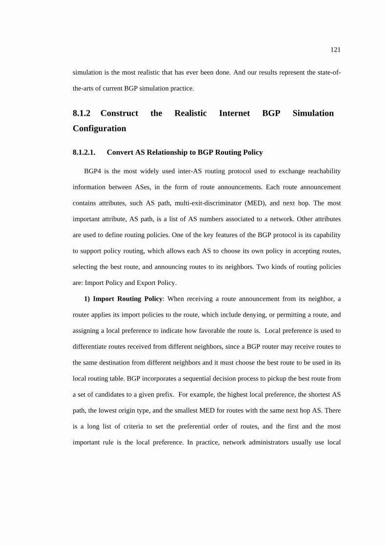
121
simulation is the most realistic that has ever been done. And our results represent the state-of-
the-arts of current BGP simulation practice.
8.1.2 Construct the Realistic Internet BGP Simulation
Configuration
8.1.2.1. Convert AS Relationship to BGP Routing Policy
BGP4 is the most widely used inter-AS routing protocol used to exchange reachability
information between ASes, in the form of route announcements. Each route announcement
contains attributes, such AS path, multi-exit-discriminator (MED), and next hop. The most
important attribute, AS path, is a list of AS numbers associated to a network. Other attributes
are used to define routing policies. One of the key features of the BGP protocol is its capability
to support policy routing, which allows each AS to choose its own policy in accepting routes,
selecting the best route, and announcing routes to its neighbors. Two kinds of routing policies
are: Import Policy and Export Policy.
1) Import Routing Policy: When receiving a route announcement from its neighbor, a
router applies its import policies to the route, which include denying, or permitting a route, and
assigning a local preference to indicate how favorable the route is. Local preference is used to
differentiate routes received from different neighbors, since a BGP router may receive routes to
the same destination from different neighbors and it must choose the best route to be used in its
local routing table. BGP incorporates a sequential decision process to pickup the best route from
a set of candidates to a given prefix. For example, the highest local preference, the shortest AS
path, the lowest origin type, and the smallest MED for routes with the same next hop AS. There
is a long list of criteria to set the preferential order of routes, and the first and the most
important rule is the local preference. In practice, network administrators usually use local

122
preference to enforce their import routing policies. According to [80], there are two general
rules:
Route Preference between Provider, Customers, and Peers: Network operators usually
assign different local preferences to routes learned from providers, customers, and peers.
Customer routes have the highest local preference, and peer routes have higher local preference
than providers.
Consistency of Local Preference with Next Hop ASes: Operators may set local
preference configuration based on prefix level or next hop AS level. Since it is easier to
maintain provider, customer, and peer preferences based on next hop AS level, most ISPs use
this approach in practice.
2) Export Routing Policy: BGP routers use export policies to decide which routes are to be
propagated to their neighbors. The policies are usually transformed directly from AS
relationships.
Exporting to a Provider: An AS can export its local routes and routes of its customers, but
can not export routes learned from its peers or providers
Exporting to a Peer: An AS can export its local routes and routes of its customers, but can
not export routes learned from its peers or other providers
Exporting to a Customer: An AS should export all routes it knows to its customers
These basic export policy rules are the direct requirement of commercial agreements. For
example, the first rule guarantees that a provider will not use its customer network to transit
traffic, and the last rule guarantees that the customer can get full Internet access through its
provider.

123
1) Generate AS level topology based on the BGP routing table
2) Decide AS relationships from the inferring
3) Setup Import Routing Policy
a. Accept all incoming routes
b. Set Local Preference according to Next Hop AS, which prefer
routes from Customer, over routes from Peer, and over routes
from Provider
4) Setup Export Routing Policy
a. To Provider: Export local and Customer routes
b. To Peer: Export local and Customer routes
c. To Customer: Export all routes
5) Pickup default/backup routers for multi-homed Ases
Figure 8.1 Procedure for Internet AS-level Topology Generation
With these heuristic rules, we can convert the inferred AS relationship to routing policies in
maBrite topology generator (Figure 8.1).
8.1.2.2. Improve the Routing Configuration with Real Routing Tables
So far, we capture the major routing policy based on AS relationship. However, AS
relationship is not the only factor for routing decisions. There are a few others details may affect
the final routing decisions, such as the multi-homed stubs AS [63] and selective Announcement
[80]. With the help of real routing tables, we can polish our topology to incorporate this
information.
Multi-home is a popular practice to provide routing redundancy and higher network
bandwidth. A multi-homed AS can have 2 or more providers, but it may prefer to use one
provide for most of the traffic, and use the other provider as a backup, in case the routing to the
first provider fails or is congested. This decision is not derivable from AS relationships;
however, it can be estimated from the real routing table data. We can get its preference by
checking all routing entries to that stub AS at observation points. We compare total number of
124
routing entries to AS S that uses the provider M and that using the provider N, and then set the
export preference of AS S.
B
A
D
C
E
p1 p2
Provider-to-Customer
Peer-to-Peer
Figure 8.2 Selective Announcement
Selective Announcement is used when the AS wants to treat parts of its network differently.
For example, as shown in Figure 8.2, the Stub AS A has two sub-networks with prefixes p1 and
p2. The AS A wants to use the provider AS B for incoming traffic of sub-network p1, and use
provider C for incoming traffic of sub-network p2. In order to achieve this effect, AS A
announces two prefixes separately; it announces only the prefix p1 to provider B, and
announces only the prefix p2 to provider C. This routing configuration is not used in our
Internet simulation, since currently the maBrite cannot create the AS configuration to generate
multiple prefixes automatically. Instead, we just pick the largest prefix and calculate its
preference as the multi-homed case above. This is the major source of error in our network
topology setup.
8.1.2.3. Scalable Routing Policy Enforcement
From the BGP routing table dumped at May 11, 2004, current Internet has about 17,000
ASes. It is still a big challenge to simulate a network of this scale, in the term of both memory
requirement and computation overhead of BGP protocols. The major memory requirement is
used to store BGP routing tables on each BGP router, and the computation overhead mainly
comes from the enforcement of routing policy.

125
7
34
6
8
13
5238
Figure 8.3 An Example of AS relationships
The routing policy is enforced through filter operation using regular expression match,
similar to the real commercial router interface. However, this approach is not very efficient and
hard to optimize for performance. For example, one AS has a routing policy that only exports
routing information of its customers to its peer. Originally this is implemented by putting a list
of all customers in the filter definition, and the filter will check the customer list one by one
when exporting a routing entry. As shown in Figure 8.3, AS 7 has a provider AS 6 and 2 direct
customers AS 13 and AS 34. However, it must list all of its customers, direct or indirect, in its
export filters (Figure 8.4). The overhead is large, for a backbone ISP with thousands of
customers, in the term of both memory consumption and computation.
Export Filter of AS 7: clause [ precedence 1 predicate [ atom [ attribute nhi_path matcher (.*)(8|13|34|38|52)$] ] action [ primary permit ]
Figure 8.4 The Export Filter using the AS list
In practice, the routing policy is enforced through the community attribute. A provider AS
assigns a special community value to all of its customers, which will be associated with all
routing entries created by the customers. Then the provider can check the community valued in

126
export filters and may assign. To mimic this approach, MaSSF implements the community
attributed and add the automatic community check/setup in the maBrite generator.
Export Filter for AS 7: clause [ precedence 1
predicate [ atom [ attribute community matcher 7] ] action [ primary permit atom [ attribute community type set value 6] ]
Figure 8.5 Export Filter using Community Attribute
The Figure 8.5 is the new export filter configuration of AS 7. The predicate matches all
routing entries with community value 7, which means they are created by its customer ASes.
All matched routing entries can be exported to AS 7’s neighbors, and the community value is
re-set to 6, which is the provider of AS 7. Similarly, AS 6 will use this community value to
enforce its own exporting policies.
Summarizing our Internet BGP simulation, we first exploit the scalability of MaSSF to
directly simulate the real Internet AS-level topology. This enables the direct comparison of
simulation results to real Internet, which is never conducted before. Then we convert the
inferred AS relationship to BGP routing configuration and enhance it with real BGP routing
table.
8.1.3 Simulation Results
From the BGP routing table dumped at May 11, 2004, current Internet has about 17,000
ASes and this generated network is simulated on a cluster with 60 Itinum-2 nodes.
There are many metrics can be used to evaluate how close is the simulated network to the
real Internet. For examples:
1) Routing paths of single-prefix-origination AS:
127
For a given studied prefix, we compare the routing paths generated by simulation and paths
observed at various BGP routers. Routing paths are influenced largely by routing decision
algorithm and policy. So by comparing paths, we can do reality check on the simulation code
and policy configuration. We will first study prefixes which are originated by single-prefix-
origination ASes. In real Internet, we can get the routing paths to these prefixes from multiple
BGP observe pointers. These paths are directly comparable to simulation results. By calculating
the percentage of simulated routing paths which are exactly the same, one hop difference, and
two hops difference, we can evaluate the reality of our routing configuration and simulation.
2) Routing paths of multiple-prefix-origination AS:
ASes which are originating multiple prefixes are not considered in the previous case.
Because for those prefixes, there may be different policies applied to them. Those policies are
purely a local decision which is not available to us. Thus it is much harder to compare
simulation results and observed behavior of those prefixes.
3) Routing Dynamics:
In real world, researchers have set Beacon prefixes, which are brought up and down
periodically. For each routing change of Beacon prefixes, we can observe and collect a set of
triggered updates. We also simulate Beacon prefixes then compare the simulated routing
updates with observed routing updates. More precisely, we compare a) # of updates; b) path
changes; c) convergence time; d) inter-arrival time distribution.
We check the routing paths to all single-prefix-origination ASes at the BGP observation
points. We use totally 44 observation points. The Cumulative Dense Function (CDF) of the
match percentage is shown in Figure 8.6, with the average of 24%. This result is much lower
than our expectation, and now it is meaningless to continue the second and third checks until we
can improve this match percentage.

128
0 10 20 30 40 50 60 700
0.1
0.2
0.3
0.4
0.5
0.6
0.7
0.8
0.9
1
Match Percentage (%)
CD
F of
Mat
ch P
erce
ntag
e
Figure 8.6 CDF of BGP Routing Table Match Percentage
Checking the simulation result, we find two major reasons for the large gap between the
simulation output and the real Internet routing table.
First, the routing error in BGP is accumulative. Due to the distributed nature of the BGP
protocol, routing decisions are made locally and then propagated to other ASes. Since every
BGP routers only export the best routing chosen by themselves, BGP routers have no global
view of the network. Any decision different to real Internet will be propagated and introduce a
large number of different routes for the other routers.
Second, the selective announcement is the major source of the error, especially in the
medium size ISP networks. Those ISP usually have a few customers AS and multiple providers,
they usually use selective announcement for traffic engineering. As we mentioned above, we
only calculate the preference of the largest prefix and use it to represent the whole AS. This can
lead to a large number of routing decision errors and then propagated to the whole Internet. To
really improve the simulation result, we must figure out how to create multiple prefixes in a
single AS and how to do selective announce automatically in maBrite.
129
8.1.4 Summary
In this study, we exploit the power of scalable network simulation in MaSSF to simulate
real AS-level Internet topology. We also construct the most realistic BGP configuration that has
ever been achieved using inferred AS relationship. This network is simulated by the MaSSF on
a 60-node cluster. We report our experimental results by comparing the simulation results
directly to real routing data. Results show there is a significant gap between simulation results
and real data, which warrants further investigation. Results show 1/4 match. As we show above,
this is mainly due the accumulative error of BGP and selective announcement. While we cannot
do much on the first issue, the later can be mitigate by supporting multiple prefixes in an AS
and advanced routing configuration support in maBrite.
8.2 Empirical Study of Tolerating DOS Attacks with a Proxy
Network
Denial-of-Service (DoS) attacks are a continuing key threat to Internet applications. In such
attacks, especially distributed DoS attacks, a set of attackers generates a huge amount of traffic,
saturating the victim’s network and causing significant damage. Proxy networks have been
proposed to protect applications from Denial-of-Service (DoS) attacks. However because large-
scale study in real networks is infeasible and most previous simulations have failed to capture
detailed network behavior, the DoS resilience and performance implications of such use are not
well understood in large networks. While post-mortems of actual large-scale attacks are useful,
only limited dynamic behavior can be understood from these single instances.
Our work exploits the unique capability of the MicroGrid, a detailed large-scale online
network simulator, to study proxy networks with real applications and real DoS attacks.
MicroGrid supports detailed packet-level simulation of large networks and use of unmodified
applications. With MicroGrid, we are able to make detailed performance studies in large
130
networks environment with complex, typical application packages and real attack software. Our
studies include networks with up to 10,000 routers and 40 Autonomous Systems (ASes) with a
physical extent comparable to the North American continent. We believe this is the first
empirical study of proxy networks for DoS resilience at large-scale, using real attacks, and in a
realistic environment.
8.2.1 Background
8.2.1.1. Distributed Denial-of-Service Attacks
Denial-of-Service (DoS) attacks have been a major security threat to typical Internet
applications[86-88], in which a central server provide services to a large number of users widely
distributed in the Internet. In a DoS attack, attackers consume scarce resource which
applications depend on, making the applications unavailable to their users.
There are two classes of DoS attacks: infrastructure-level and application-level attacks.
Infrastructure-level attacks directly attack the service infrastructure, such as the network and the
hosts of the application services, for example, by sending floods of network traffic to saturate
the network of the application services. On the other hand, application-level attacks denial-of-
service applications by exploiting weakness in application-level protocols, for example, by
overloading application services with abusive workload or by sending malicious requests
causing application services to crash.
Infrastructure-level attacks only require the knowledge of applications’ network address, i.e.
IP address. Meanwhile, application-level attacks are tightly-coupled with application-level
protocols and do not require applications’ IP addresses.
Distributed Denial-of-Service (DDoS) attacks are large scale DoS attacks, which typically
involves a large number of “zombies”. There are two stages in such attacks. First, attackers
build zombie networks by compromising Internet hosts and installing zombie programs.

131
Second, attackers control the zombies to DoS the victim. Both infrastructure and application-
level DoS attacks can be used in the second stage. Automated DDoS toolkits, such as
Trinoo[89], TFN2k and mstream [90], and worms, such as CodeRed [91, 92], have been used
for automation, enabling large scale attacks.
Our study focuses on distributed infrastructure-level DoS attacks.
8.2.1.2. Proxy Network Approach
Internet
Application
Attackers
Proxy Network
Users
edge proxy proxy
Figure 8.7 DoS-Tolerant Proxy Network
Overlay networks have been used to protect applications from DoS attacks [93-97]. Figure
8.7 shows a generic proxy network encompassing most of the proposed approaches. It shows a
conceptual view of the proxy network from two perspectives. Proxies run on a resource pool
with a large number of interconnected hosts, e.g. Internet hosts; proxies and applications form
an overlay network by having logical connections tunneling application-level traffic among
proxy nodes. The essence of the proxy network approach is to allow communication between
users and applications without revealing the applications’ low-level network address, e.g. IP
address. Applications do not publish their own IP addresses. Instead the addresses of a number

132
of edge proxies are published, and these proxies are used to communicate (via other proxies)
with the application.
Since only application level traffic is delivered inside the proxy network, once an
application’s low-level network address is hidden from attackers, direct infrastructure DoS
attacks on the application are avoided. Furthermore, the proxy network is widely distributed in
the network and highly redundant, so that it is DoS-resilient and it can shield the applications
from DoS attacks.
8.2.2 Problem Definition and Approach
8.2.2.1. Problem
We have little understanding of the performance or effectiveness of proxy networks to
provide DoS resilience in large-scale realistic networks. To date, studies of these problems have
been limited to theoretical analysis and small-scale experiments. They cannot capture real
complex network structures, real temporal and feedback behavior of network and application
protocols, and detailed network dynamics, such as router queuing and individual packet drops.
All these have important impact on system performance.
Thus, we still do not have answers to many key questions about the viability and properties
of these proxy approaches.
1) With real complex network structures and protocol behavior, can proxy networks tolerate
DoS attacks? In particular, in large realistic networks, under various attack scenarios, how
much can proxy networks mitigate the impact of DoS attacks on users’ experienced
performance? What are the key parameters to achieve effective and efficient resilience? How
does this capability scale up when proxy networks grow in size?
2) What are the basic performance implications of proxy networks? How do they affect
users’ experienced performance for real applications in large-scale realistic networks?

133
8.2.2.2. Challenges
To answer these questions, network simulation is necessary, since you cannot do large-scale
DOS experiments on real Internet and or a small testbed. However, simulation for DOS attacks
presents large challenges on the capability of network simulator.
First, the network simulator must be scalable to support simulation of large network with
huge DOS traffic. To make the study results applicable to real Internet environment, the proxy
network should be large enough. Also, this proxy network should be widely distributed in the
network, and it presents a requirement on number of routers in the simulated network. Besides
the large network size, we also expect the large DOS traffic from the attacking module. Since
the basic approach for DOS attack is to saturate the network link, we expect the traffic of a few
Gbps attacking traffic in the simulated network.
Second, it requires low level details to understand the attacking effect on applications
performance. For example, the slow-start effect of TCP congestion window control, the AIMD
policy on packet drop, and even the jitter due to the router queuing delays will greatly affect the
proxy network and application’s performance. Without this packet level detailed network
simulation, it is impossible to study these behaviors. Because DoS attacks exercise extreme
points of network behavior, correct modeling of such detail is important for realistic studies. In
this context, we study the performance and DoS resilience of the generic proxy network
approach.
Third, it is important to model real temporal and feedback behavior of network and
application protocols and their interaction with other network traffic. This is difficult without
online network simulation capability. Online network simulation can also help to capture the
subtle details in the proxy network implementation, which is quite important to the final
performance of the application.

134
Due to these challenges, there are no solid answers to the questions above. Existing network
simulator are either limited in scalability or in the simulation details.
8.2.2.3. Approach
MicroGrid enables us to study these problems in a straightforward way, which cannot be
easily achieved before. MicroGrid creates an Internet-like large-scale virtual network
environment, and allows unmodified applications running on it. We built a proxy network
prototype and deployed it along with a real application and real user programs into the
MicroGrid virtual environment. We build a large zombie network in the virtual environment
running a real DDoS toolkit to generate attack traffic. This allows us to do controlled
experiments with different proxy network configurations and different attack scenarios, and
study the questions above.
Details of our approach include:
1) Use of a large-scale, high-fidelity packet-level online network simulator –
MicroGrid – to simulate large-scale realistic network environment, which include
up to 10,000 routers and 40 ASes comparable to the size of large ISPs.
2) A real proxy network implementation and real applications deployed together in
the MicroGrid virtual environment.
3) A large zombie network of 100 zombies and a real distributed DoS toolkit to
generate attack traffic. It supports controlled experiments with various attack
scenarios.
4) A tree proxy network topology, rooted at the application with edge proxies at the
leaves providing user access. The number of edge proxies is the width of the tree,
and the number of hops from root to leaves is the height. For a localized

135
application implementation, the tree corresponds to subset of links that would be
exercised in all proxy networks.
5) Systematic study of a range of attacks, proxy network configurations, application,
and resilience strategies.
We systematically study users’ experienced performance using a range of proxy network
topologies to understand the basic performance impacts of proxy networks; then we generate a
range of attack scenarios with different attack magnitude and distribution, and systematically
study their impact on users’ experienced performance with proxy networks of different sizes to
understand proxy networks’ DoS-resilience capabilities and scalability.
8.2.3 Experimental Environment
8.2.3.1. Software Environment
There are four software components used in the experiments: a proxy network prototype
implementation, apache web server as the application, a web testing tool “siege” to simulate
user access, and a DDoS attack tool “Trinoo”.
1) Proxy Network Prototype Implementation
The proxy network is a generic overlay network composed of proxy nodes. It can be
configured to support any topology and extended to support any routing algorithm. Proxy
nodes have unique identifiers, and act as routers. Each pair of neighboring proxies maintains a
TCP connection. When a proxy starts, it connects to its neighboring proxies according to the
specified topology information and some bootstrap location information of their neighbors.
Messages can be routed inside the proxy network following any given routing algorithm.

136
Proxy Network
Application
User
Edge Proxy Internal Proxy
App Proxy
Topology Spec Routing Algorithm
Figure 8.8 Generic Proxy Network Prototype
The proxy network supports all TCP applications transparently. We use the DNS scheme
used by content delivery networks [98] to direct user access to proxies.
As shown in Figure 8.8, edge proxies listen to user connection requests, and encode
application traffic into messages which are routed via the proxy network to the application. At
the exit of the proxy network, application proxies (proxies that directly connect to the
application) decode the messages, establish new connections to the application if necessary, and
send the data to the application. The TCP connections among proxies are persistent and shared
among users.
2) Application Service
We use Apache web server as a representative application front-end. Since we focus on the
network impact of DoS attacks, specific details of the application logic at the back-end are not
critical. Here we use Apache server to serve files of different sizes as a representative scenario.
3) User Simulator
We use siege – a web test toolkit – to generate user requests. Siege can generate web
requests based on a list of URLs and measure the response time for each of the requests. This
allows us to simulate user access and collect statistics which characterize user experienced
performance.
4) DDoS Attack Toolkit

137
The attack tool used in experiments is the simTrinoo, which is a simulation module in
MaSSF to mimic the behavior of the Trinoo attack tool. Based on two concerns, we do not use
the real Trinoo program directly. First, due to the huge traffic created by attackers, the overhead
of using Trinoo is quite large, especially in the Agent module of the simulator, which accepts
and dispatches requests inside the simulator. It will affect the scalability of the whole system.
Second, the logic of the Trinoo is so simple that we can easily reproduce the same traffic pattern
inside the simulator using a traffic generator. Comparing to the simTrinoo, it will not bring any
benefits to the accuracy of our simulation results.
Just like the Trinoo program, each simTrinoo attacker maintains a list of victims.
Periodically, it randomly picks up one victim and sends out UDP attacking packets to it. By
controlling the sleep between every two attacks and setting the victim list on every attacker, we
can control the attacking traffic enforced on each proxy node.
8.2.3.2. Simulation Setup
The proxy network, apache server, siege programs and simTrinoo attackers are deployed in
the MicroGrid simulated network environment. The maBrite topology generator is used to
generate Internet-like Power-Law network topologies. We use two virtual networks in our
experiments. One includes 1000 routers and 20 ASes, and the other includes 10,000 routers and
40 ASes, which is comparable to the size of a large ISP network. Both networks span a
geographic area of 5000 miles by 5000 miles, which is roughly the size of the North American
continent. This physical extent determines link latencies. OSPF routing is used inside ASes,
and BGP4 is used for inter-AS routing.
Our network simulator is running on an 8-node dual 2.4GHz Xeon Linux cluster with 1G
main memory each, connected by a 1Gbps Ethernet switch. The proxy and siege processes are

138
running on another 24-node dual 450MHz PII Linux cluster with 1G main memory each,
connected by a 100Mbps Ethernet switch. These 2 clusters are connected with a 1Gbps link.
8.2.4 Experiments and Results
To answer the questions stated in Section 8.2.2, we conducted three sets of experiments:
proxy network performance evaluation, proxy network resilience against DDoS attacks using
simple redundancy schemes and proxy network resilience using fail over schemes.
8.2.4.1. Proxy Network Performance
To understand the performance implication of the proxy network approach, we compare the
user-observed service performance between the case where users directly access the application
and the case where a proxy network is used. We use a sample of 100 users randomly chosen
from the simulated network described in Section 8.2.3. Users choose edge proxies based on
proximity.
We use a simple heuristic to deploy a proxy network. Edge proxies are uniformly
distributed in the simulated network. Application proxies are placed on hosts physically close
to where the application service is. All the other proxies are evenly distributed between edge
proxies and application proxies. This heuristic tries to align a proxy network to the underlying
network to avoid long detours in overlay routes. It is straightforward to implement this heuristic
for proxy networks whose topology is a tree, which is the case used in our experiments.
Figure 8.10 shows the results for a tree-topology proxy network with about 200 proxies, 64
of which are edge proxies. The X-axis is the response time for a user to download a given size
file (1.5KB or 100KB) either directly from the application service or via the proxy network.
The Y-axis is the Cumulative Density Function (CDF) of user-observed response time over the
user population.

139
Proxy Network
Application
User
Figure 8.9 Direct Access vs. Proxy Network
Surprisingly the proxy network greatly improves performance. For small requests (e.g.
1.5K), the 50-percentile response time is reduced by half, and for medium size requests (e.g.
100K), the improvement is even more significant. However, the performance gap between the
two cases becomes smaller for large files (e.g. >1MB). There are two main reasons for this:
First, proxy network improves connection set up time. As shown in Figure 8.9, there are
established TCP connections among proxies. For each virtual connection between a user and
the application, instead of establishing a long TCP connection between the user and the
application, two shorter TCP connections are established: a connection from the user to the edge
proxy it uses and a connection from the corresponding application proxy to the application.
Both of these are short connections, because application proxies are close to the application
service, and users choose edge proxies based on proximity. Second, the TCP connections
among proxies are persistent, and in most cases the TCP congestion windows for those
connections have already been fully opened. It no longer needs TCP slow start phase to grow
the congestion window over multiple round trips to complete a data transfer. For medium size
requests (e.g. 100KB shown in Figure 8.10), this effect is most prominent.
0 0.1 0.2 0.3 0.4 0.5 0.6 0.7 0.8 0.90
0.1
0.2
0.3
0.4
0.5
0.6
0.7
0.8
0.9
1
Response Time (seconds)
CD
F O
ver U
ser P
opul
atio
n
Performance Implication of ProxyNetwork (1.5KB file, mean)
W/O Proxy NetworkW/ Proxy Network

140
0 0.5 1 1.5 2 2.50
0.1
0.2
0.3
0.4
0.5
0.6
0.7
0.8
0.9
1
Response Time (seconds)C
DF
Ove
r Use
r Pop
ulat
ion
Performance Implication of ProxyNetwork (100KB file, mean)
W/O Proxy NetworkW/ Proxy Network
0 2 4 6 8 10 12 140
0.1
0.2
0.3
0.4
0.5
0.6
0.7
0.8
0.9
1
Response Time (seconds)
CD
F O
ver U
ser P
opul
atio
n
Performance Implication of Proxy Network (1MB file)
Direct Application AccessAccess via Proxy Network
Figure 8.10 Proxy Network Performance Implication
For these reasons, having a proxy network can potentially improve the user-observed
application performance, and the following principles should be considered in the deployment
of proxy networks. Each overlay hop (i.e. RTT between neighboring proxies) should be kept as
short as possible. Edge proxies should be widely distributed to be close to users, and
application proxies should be put close to the application.
In this experiment, the online simulation capability of the MicroGrid enable use to study the
application performance directly in large networks. The packet level detailed simulation in the
MicroGrid is also critical to capture the application performance, which depends the accurate
modeling of TCP hand-shaking and slow-start.

141
8.2.4.2. DoS-Resilience of Proxy Networks
To explore the DoS-resilience capability of proxy networks, we study user-experienced
performance under a range of attack scenarios with or without proxy networks. We use the
same proxy network, which contains 192 proxies (64 edge proxies), in the simulated network
with 20 ASes and 1000 routers. In addition, we constructed a DDoS network, which contains
100 Trinoo daemons randomly distributed in the network.
Our first experiment explores whether a proxy network can really protect an application
from DoS attacks. Our second experiment studies the DoS-resilience capability of the proxy
network under two large-scale attack scenarios: spreading DoS attacks where attack load is
distributed evenly on all the edge proxies and concentrated DoS attacks where attack load is
concentrated on a subset of edge proxies to saturate their incoming links. Our final experiment
studies the scalability of proxy networks with respect to DoS-resilience, by varying the size and
width of proxy networks.
1) Can a proxy network protect applications?
0 1 2 3 4 5 6 7 8 9 100
0.1
0.2
0.3
0.4
0.5
0.6
0.7
0.8
0.9
1
Response Time (seconds)
CDF
Ove
r Use
r Pop
ulat
ion
Effectiveness of Proxy Networks
no attack (with proxies)no attack (direct application access)250Mbps attack (with proxies)250Mbps attack (direct application access)
Direct App Access, No Attack
Figure 8.11 DOS-Resilience of Proxy Network
We compare the impact of a DoS attack cast on the application and the proxy network. In
our experimental setting, the application service is connected by a 250Mbps link, and each edge
proxy is connected by a 100 Mbps link. Figure 8.11 shows the CDF for user-observed service
response time of 100KB request size in scenarios with or without a proxy network. The results

142
show that a 250Mbps attack on the application significantly increases service response time
(about 10x) and the application becomes unusable. However, when a proxy network is used,
the attack has no observable impact on the user experienced performance. The reason is
straightforward. By having a collection of edge proxies to dilute the impact of attack, a proxy
network has a greater capacity than the application, thereby not as easily being saturated.
2) How large an attack can a proxy network resist?
To investigate how well a proxy network can tolerate DoS attacks, we launch both
spreading and concentrate DoS attacks on the proxy network described in Section 8.2.3, which
has 64 edge proxies and 192 proxies in total. Each of the edge proxy has a 100Mbps uplink. In
both cases, we vary the aggregated attack magnitude from 3.2Gbps to 6.4Gbps. In this
experiment, users do not switch proxies during attacks.
In the case of spreading DoS attacks, Figure 8.12 shows that when attack magnitude is no
more than 6.0Gbps (recall that the aggregated uplink capacity for all the edge proxies is
6.4Gbps), more than 95% of the users observe no significant performance degradation --the
DoS attack has been successfully tolerated. The reason for this is that the edge proxies
successfully dilute attack, and even under heavy attack loads, most of the edge proxies still have
sufficient capacity left to serve user requests. Figure 8.12 also shows that when attack load
reaches 6.4Gbps, all the edge proxies are saturated, significant performance degradation occurs
for all users.

143
0 1 2 3 4 5 6 7 80
0.1
0.2
0.3
0.4
0.5
0.6
0.7
0.8
0.9
1
Response Time (seconds)
CD
F O
ver U
ser P
opul
atio
n
Spreading Attack, 64-Edge Proxy Network (100KB Request)
proxy network, no attack3.2 Gbps Attack6.0 Gbps Attack6.4 Gbps Attack
Figure 8.12 Redundancy to Spreading DoS Attack
Internet
Edge proxy A
OC3 uplink
Edge proxy B
User
Attack Traffic
Attack Traffic
Figure 8.13 Correlation among Proxies and Users
More interesting, we can see large performance degradation for a small fraction of users
(<5%) when the attack magnitude is 6.0Gbps. It is due to the correlation among proxies and
users (see Figure 8.13). Two edge proxies A and B share an uplink of OC3 (155Mbps). Before
attack traffic saturates both proxies’ local links (100Mbps), the shared OC3 link gets congested
first. Therefore, users who use these two proxies and users who are in the same network as
these proxies will be affected. This effect limits the effectiveness of proxy network. Thanks to
the accurate simulation of the MicroGrid even under heavy traffic, we can capture this
phenomenon in the simulation.
Figure 8.14 shows the case of concentrate attacks, where attack load is concentrated on a
subset of proxies. In this case, attack traffic saturates part of the proxy network and a

144
significant percentage of users are affected due to congestion and packet loss. This effect is
more prominent when attack load is higher than the proxies’ capacity (e.g. 4.0Gbps attack on 32
proxies).
0 1 2 3 4 5 6 70
0.1
0.2
0.3
0.4
0.5
0.6
0.7
0.8
0.9
1
Response Time (seconds)
CDF
Ove
r Use
r Pop
ulat
ion
Concentrate Attack (100KB Request Size)
no attack3.2 Gbps Attack on 32 Proxies4.0 Gbps Attack on 32 Proxies6.0 Gbps Attack on 48 Proxies6.0 Gbps Attack on 60 Proxies
Figure 8.14 Resilience to Concentrate DoS Attack
We observe that parts of the proxy network are not under direct DoS attacks; therefore if
users can switch to edge proxies not being attacked, the performance can be potentially
improved. We repeat the concentrate DoS attack experiment, and let users switch to the closest
proxy not being saturated. Figure 8.15 shows the CDF of user-observed performance.
Compared with Figure 8.14, the performance has been significantly improved. For comparison,
Figure 8.15 also plots the baseline case where users directly access the application without
attack traffic. It shows that even under high attack load (e.g. 6.0Gbps) the proxy network can
still maintain slightly better performance than direct application access without attacks for most
users. Therefore proxy networks can effectively resist DoS attacks.
0 1 2 3 4 5 6 70
0.1
0.2
0.3
0.4
0.5
0.6
0.7
0.8
0.9
1
Response Time (seconds)
CDF
Ove
r Use
r Pop
ulat
ion
Performance Implication of Proxy Network (100KB file)
no attack with proxy network3.2 Gbps Attack on 32 Proxies4.0 Gbps Attack on 32 Proxies6.0 Gbps Attack on 48 Proxies6.0 Gbps Attack on 60 ProxiesDirect Application Access
No Attack, direct application access
Figure 8.15 Resilience to Concentrate DoS Attacks with Proxy Switching

145
This experiment demonstrate the capability of the MicroGrid to simulate large network
accurately even under heavy traffic. With 6.4Gbps attacking traffic and average 15 hops per
stream, we are simulating a 1000 routers network with about 100Gbps traffic flowing in the
network.
3) How does proxy network size affect DoS-resilience?
Finally, we explore how varying the size (width) of the proxy network affects DoS
resilience. This is an important scaling property of the proxy network, showing how effective
we can resist larger scale DoS attacks by building larger proxy networks. The goal of our
experiment is to evaluate the amount of attack load proxy networks can withstand for a range of
proxy network widths. It is hard to directly measure the maximum attack load a proxy network
can tolerate. Instead, we set the attack magnitude to be 95% of the proxy network’s capacity,
and measure the user-observed performance. We define the capacity of a proxy network to be
the sum of the link capacity of its edge proxies. For example, if the proxy network has 16 edge
proxies and each edge proxy has a 100 Mbps uplink, then its capacity is 1.6Gbps and the
aggregated attack magnitude is 1.52Gbps.
Proxy network scaling results are shown in Figure 8.16. The X-axis is the number of edge
proxies in the proxy network (they all have height 3), and the Y-axis is the user-experienced
service response time for a certain percentile of users. We can see that for up to 95 percent
users, the curves stay horizontal and less than 2 seconds (recall from Section 8.2.4.1 that the 95
percentile performance for direct application access without attacks is 2 seconds). If we define
95% users not being affected by DoS attacks as successful DoS resilience, then the amount of
attack traffic can be tolerated grows linearly with the size of the proxy network.

146
0 10 20 30 40 50 60 700
0.5
1
1.5
2
2.5
3
3.5
4
4.5
Number of Edge Proxies
Use
r Exp
erienc
ed R
espo
nse
Tim
e (S
econ
ds)
90 Percentile92 Percentile95 Percentile97 Percentile
Figure 8.16 Resilience and Proxy Network Size
This experiment is a good demonstration of the flexibility of the MicroGrid resource
configuration. It can easily construct proxy networks and deploy them to the virtual network.
With the MicroGrid, it is possible to study various network configuration and application
scenario under controlled environment.
8.2.5 Conclusion
Our work provides the first detailed and broad study of DoS resilience with proxy network
in large-scale realistic networks. The key is that we exploit the unique capability of the
MicroGrid to simulate a realistic large-scale network (comparable to several large ISPs). We
use a generic proxy network and deploy it in a large simulated network using typical real
applications and DoS tools directly. We study detailed system dynamics under various attack
scenarios and proxy network configurations. The major conclusion is that, in realistic large
network environments, proxy networks can have great performance potential and scalable DoS-
resilience capability. It is a promising approach to DoS defense. These experiments and the
conclusion are not possible without the scalable, accurate online simulation provided by the
MicroGrid.

147
8.3 Summary
In this chapter, the MicroGrid toolkit is successfully used on two real network related
studies, none of them is possible without the MicroGrid. These experiments demonstrate the
unique capabilities of the MicroGrid which are critical to the success, including:
1) Scalability. This is required by the simulation of the whole Internet AS-level topology
and large attack traffics.
2) Accurate and detailed simulation. The DoS study of proxy network requires very detailed
network modeling, including TCP slow start, TCP AIMD congestion control, and router
queuing and dropping.
3) Online simulation capability. The proxy network evaluation is not possible without the
online simulation capability. Furthermore, our online simulation helps us to detect and fix a
batch bugs in the proxy network implementation.
4) Flexible on virtual grid configuration. The DOS study experiments require flexible
deployment of a large number of proxy and user hosts.

148
Chapter 9 Related Work
In this chapter, we discuss the most related work, current research on network emulation for
application performance studies. Those are all interesting because they are quite similar to our
approach in supporting direct execution of applications. However, there is still a major
difference between them and the approach used in the MicroGrid, and we want to point them
out clearly. In Section 2.1 we have discussed other related work in application performance
modeling.
We will briefly describe their approaches in Section 9.1 and compare them to the MicroGrid
in Section 9.2. Then we will summarize the difference at Section 9.3.
9.1 Network Emulation Projects
Several recent research efforts are most similar to the MicroGrid, including ModelNet [35],
Netbed [36], Maya[99], and Albatross [100].
9.1.1 ModelNet
The ModelNet [35] project at Duke University (and now at UCSD) is a software emulation
environment on a cluster. The ModelNet simplifies network topology as a network of pipes,
calculates the shortest-path routing, and then maps the resulting network of queues onto a set of
emulation cores. Network IP packets from real applications running on end hosts will be routed
through one or more cores. The core will subject each packet to delay, bandwidth, and loss
characteristics, according to the target topology. ModelNet moves packet hop-by-hop in the
topology and each hop is represented by a pipe with a packet queue. Whenever a packet enters a

149
pipe queue, the emulator will calculate the queuing and link delay and forward the packet to the
next hop, after desirable delay, if it is not dropped due to a queue overflow, randomized loss, or
a RED policy. Thus ModelNet can track the effects of congestion and competition among
competing packets.
Key differences to the MicroGrid include:
1) The MicroGrid models real network entities and their behaviors, while the ModelNet
simplifies them to pipes and queues. In the MicroGrid, every router has fully
functional Network Interface Cards (NIC), packet buffer queue, and protocol stack of
IP, TCP, OSPF or BGP. Thus it is easy for the MicroGrid to incorporate detailed
routing configuration and make dynamic routing selection as in the real Internet. The
ModelNet, however, has to load a pre-calculated routing path at the emulation startup
time, lookup the static routing path for every packet entering the emulators, and then
move it through all hops in that path. While this approach reduces the simulation
overhead greatly, it is not easy to implement dynamic routing without major
modification.
2) The MicroGrid supports scaling of all resources and performance ratio precisely, while
the ModelNet must follow the real-time emulation requirement and has no modeling of
computation resources. This difference gives the MicroGrid more flexibility in
simulating various, and even future, network and resources speed and ratio.
3) The MicroGrid uses advanced load balance and scaled real-time execution for
scalability, while the ModelNet mainly counts on approximation and some load
balance improvement. The Distill phase in ModelNet transfers an original network
topology into a network of pipes, and it can simplify the network, if the emulator is not
fast enough to keep up the real-time execution, trading accuracy for reduced emulation
cost. In contrast, the MicroGrid uses full-scale detailed packet-level simulation based

150
on a distributed discrete-event simulation engine. As for the load balance problem,
ModelNet[101] uses the greedy k-cluster algorithm: for k nodes in the core set,
randomly selects k nodes in the virtual topology and greedily selects links from the
current, connected component in a round-robin fashion. They also use an approach
similar to the MicroGrid PLACE mapping, but it is focused on minimizing Network
traffic between cores. While there are continued improvement on scaling and
possibility of emulating a 10,000 nodes network[102], the largest emulation on
ModelNet we know has 4000 virtual nodes running on 9 cores [101].
4) The MicroGrid has higher cost on simulating every packet movement, but it can be
used on publicly shared general Linux cluster systems, while the ModelNet required
dedicated customized FreeBSD clusters. This may seem to be a trivial user interface
issue, but it has a big impact in practice; since users of the MicroGrid can do much
larger scale simulation on publicly shared large cluster systems (such as TeraGrid[2]).
9.1.2 Netbed/Emulab
The Netbed/Emulab [36] project, developed at Utah University, uses a set of real routers,
switches and configurable software routers to emulate wide area network. Netbed can also
integrate simulation, wide-area network testbeds, and emulation into a common framework.
This framework provides abstractions, services, and namespaces common to all, such as
allocation and naming of nodes and links. By mapping the abstractions into domain-specific
mechanisms and internal names, Netbed masks much of the heterogeneity of the three
approaches. The Netbed users can benefit from choosing appropriate modeling approaches for
their special requirements, even in a single simulation experiment.
Key differences to the MicroGrid include:

151
1) Netbed requires real-time emulation, which has the benefit of quick simulation. At the
same time, the real-time execution requirement is also a limit on scalability. The
MicroGrid uses scaled real-time execution and can achieve better scalability with the
cost of slower simulation.
2) Netbed also provides little to the experiment designer in the way of detailed control of
resource speed and modeling. Regardless how many resources are dedicated in the
Netbed resource pool, the resource type and number are still limited, when compared to
possible virtual network configurations. The user has to select and configure whatever
available physical resources to approximate the target virtual network, which will lead
to possible inaccuracy. In practice, Netbed's assign [103] automatically maps virtual
topologies which include endpoint resources, as well as network structures, onto a
heterogeneous combination of routers, switches, and computers. In contrast, the
MicroGrid provides accurate resource modeling, and has no inaccuracy introduced by
this kind of approximation.
3) Netbed provides no load balance solution. While the assign automatically chooses
specific endpoint and network resources to optimize their quantity subject to the
constraints, load balance is not its direct focus. Instead, the MicroGrid provides
advanced load balance mechanism for better scalability.
4) The scalability is also limited by the available physical resources in the Netbed resource
pool. The largest automatically-configured Netbed experiment [104] of which we are
aware has 520 virtual nodes (routers) mapped to 44 PCs. The MicroGrid can use any
publicly available Linux cluster systems and conduct much larger scale simulation.
152
9.1.3 Maya
The Maya [99] Project at UCLA also provides a network modeling framework for
emulating distributed applications. Like ModelNet and Emulab, Maya supports direct execution
of applications, and also has the real-time execution requirement.
Key differences to the MicroGrid include:
1) The unique feature of Maya is that it can integrate two disparate modeling approaches
into a unique framework; that is, the discrete-event model and the analytic model. The
analytic model uses the fluid flow based TCP model [21] for network simulation. As
its name suggested, the fluid model treats TCP traffics as fluids, and it derives a set of
ordinary differential equations (ODE) to model the rate of traffic changes and
queuing process at routers. Unlike the discrete-event model, there is no packet or
event in a fluid model; and it only needs to solve the ODE periodically. Thus it can
dramatically reduce the overhead of network simulation. The MicroGrid only uses the
discrete-event model.
2) With cost of fidelity, Maya has the potential to support a very large network
simulation. It is suitable for simulating backbone network with high volume of traffic
for traffic engineering and real-time monitor and control, but it cannot capture the
detailed packet movement, which is critical to application performance. The
MicroGrid, however, does not trade fidelity for scalability. It uses packet-level
detailed simulation to capture all the details of network protocols and router behaviors.
3) While it is shown that speed of fluid flow simulation can support real-time execution
in long term, the periodical invocations of the computation intensive ODE solver
causes the packets to miss their real time deadline repeatedly. This hurts the accuracy
of real-time application emulation and limits its scalability. The largest simulation
they have reported so far is just 60 nodes [99].

153
4) Maya has no support for resources modeling either, which leads to little control on
application execution. The MicroGrid is an integrated simulation framework that
provides simulation for all resource and network components.
9.1.4 Panda in Albatross
The Albatross [100] Project provides programming environments for high-performance
Grid computing. To facilitate investigating the application performance in wide-area networks,
they developed a Panda WAN emulator as part of their communication library. This Panda
WAN emulator works in a way similar to that of the dummynet emulator [33].
Key differences to the MicroGrid include:
1) However, thanks to the tightly couple with the communication library, one unique
feature of the Panda emulator is that it can run parallel applications on a single parallel
machine with only the wide-area links being emulated. The actual emulation of WAN
behavior only models the network delay and bandwidth and cannot catch the network
queuing and congestion status. Like all other emulation projects, it is also limited to
real-time execution, and has no control on computation resources. The MicroGrid,
instead, uses binary interception to redirect all network related functions call to the
simulator. We do not distinguish between local area network and wide area network.
While it is not clear if the accuracy of whole simulation will be affected by not
modeling the local area network, it can definitely reduce the simulation overhead.
2) More accurately, the Panda is not a general network emulator like the MicroGrid, due
to the fact that it does not provide multiplex of multiple virtual machines on a single
physical resource. This makes it quite limited on the resources configuration that it
can emulate. The largest simulation reported is using a 64 nodes cluster to simulate a
154
distributed application with 64 nodes [100]. This is far beyond the scalability of the
MicroGrid system.
9.2 Novelties of the MicroGrid Approach and Capability
While we have mentioned the important differences between these emulation systems and
the MicroGrid above, it is clearer to list all novelties of the MicroGrid approach and capability
together.
First, all of these systems require real-time execution, and the MicroGrid is unique in
providing support for scaled real-time simulation and computation resource modeling. As we
have discussed in Section 5.3, this feature is the base of coordination between multiple
simulation modules, and it can also improve simulation accuracy and scalability. This capability
does not come as an accidence; instead, it requires an implementation of TCP protocol stack in
the network simulator, which is quite labor-intensive and slows down the simulation speed.
With the support of the computation resource simulation discussed in Section 5.2, the
MicroGrid can simulate grid environments with a wide range of heterogeneous resources and
various compute and network speeds ratio. For example, the MicroGrid can accurately simulate
fast network and resources which are still not currently available. Moreover, it can also
accurately simulate various network and resource ratio without the limitation of available
physical resources. None of those features are possible with any of the emulation systems listed
above.
Second, the network modeling in these emulation systems either use approximation models
or have limited scalability. These approximations reduce the cost (compared to the MicroGrid’s
global synchronized simulation) to achieve faster execution. The MicroGrid is unique in that it
uses realistic network topologies, realistic routing protocol, detailed packet level simulation, and
background traffic from aggregated large numbers of traffic flows. The MicroGrid does not

155
make tradeoffs between accuracy and scalability in network simulation, and it tries to provide
the most accurate simulation result possible. With scalable hardware like modern clusters, we
demonstrate that this approach is feasible, even to simulate a large ISP network.
Third, the MicroGrid has the most advanced support for network routing. It uses OSPF for
intra-domain routing and BGP for inter-domain routing. This can help the MicroGrid to provide
realistic network routing selection and dynamic routing reaction under network congestion or
link failure. This is important when studying the application performance under extreme and
unusual conditions. All other projects just use pre-calculated static routing information. For
example, the ModelNet uses pre-calculated shortest routing path based on static network
topology. Static routing has much less overhead in simulation execution, and the routing table
size (not the real emulation yet) can scale to hold a network with about 10,000 nodes[102].
However, it is difficult for those projects to introduce dynamic routing into the simulation.
Fourth, advanced load balance is also a critical feature of the MicroGrid. Load balance is
known to be an important and hard problem for the scalability of distributed network
simulations or emulations; However, there are only a few efforts in network
simulation/emulation community to solve this problem. Many projects, including the Maya and
Albatross, use either manual partitioning or simple graph partitioning based on network
topology. ModelNet[101] uses the greedy k-cluster algorithm: for k nodes in the core set,
randomly selects k nodes in the virtual topology, and greedily selects links from the current
connected component in a round-robin fashion. They also use an approach similar to our
PLACE mapping, but this is focused on minimizing Network traffic between cores. Netbed's
assign [103] maps virtual topologies which include endpoint resources, as well as network
structures, onto a heterogeneous combination of routers, switches, and computers. Critical
issues are time to compute mapping, physical resources used, and sufficient link capacity. Thus,
assign chooses specific endpoint and network resources to optimize their quantity subject to the

156
constraints. Load balance is not a direct focus. During the time of this dissertation writing, we
noticed that the BGP++[105] is also using graph portioning approaches for load balance in its
distributed network simulation.
9.3 Summary
Even with similarity in supporting real application execution, the MicroGrid is
distinguished from other emulation project for goal, accuracy and scalability.
The key difference between MicroGrid and these emulation approaches is the scaled real-
time execution and the more flexible application control. The scaled real-time execution
relieves us from the real-time limitation of emulation, and provides much larger scalability and
accuracy. Since the MicroGrid is an integrated simulation of network and grid resources, it
provides resource modeling and flexible control on application execution. Combined with the
scaled real-time execution, the MicroGrid can study various, even future, hardware speeds and
ratios.
Beside our novel approach for virtual grid modeling, our automatic load balance
mechanisms also provide major scalability advantage over other systems. The realistic packet-
level network simulation with O(104) routers enables accurate grid dynamic study at
unprecedented scale and great opportunities for new insights.

157
Chapter 10 Summary and Future Work
Having presented and evaluated the scaled real-time online simulation and the load balance
algorithms for better scalability, we now summarize our work and list the impact of our work on
simulation research. After that, we enumerate some limitations on our system and possible
directions of future work.
10.1 Summary
The increasing acceptance of grid computing in both scientific and commercial
communities presents significant challenges for understanding the performance of applications
and resources together. The associations between applications and resources are no longer static,
and dynamic resource sharing and application adaptation further complicate the situation.
To meet the emerging modeling needs and to enable growth in understanding the dynamic
properties of grids, we have developed the scaled real-time online simulation mechanism and
implemented it in a toolkit called the MicroGrid. The MicroGrid enables accurate and
comprehensive study of the dynamic interaction of applications, middleware, resource, and
networks. The MicroGrid creates a virtual grid environment – accurately modeling networks,
resources, the information services (resource and network metadata) transparently. Thus, the
MicroGrid enables users, grid researchers, or grid operators to study arbitrary collections of
resources and networks.
Accuracy and scalability are the two major challenges in virtual grid simulation. In
computation resource modeling, we use the soft real-time process scheduling, which can
provide accurate computation resource simulation efficiently. This technique has few

158
requirements; it can be used on any OS that supports POSIX.5 thread system. For network
modeling, we use packet-level online network simulation based on discrete-event simulation
engine, enhanced with OSPF and BGP routing protocols. With the support of transparent live
application traffic interception and the coordination through scaled real-time execution, real
application can be executed directly on a virtual grid environment; both computation and
network behaviors can be modeled accurately. To validate our approach and the MicroGrid
implementation, we present experimental results with applications, showing that the MicroGrid
not only runs real grid applications and middleware, but it accurately models both the
underlying resource and network behavior.
We also study a range of techniques for scaling a critical part of the online network
simulator to the simulation of large networks. These techniques employ a sophisticated graph
partitioner, and a range of edge and node weighting schemes exploiting a range of static
network and dynamic application information. By carefully mapping the virtual network to
physical resources using multi-objective graph partitioning algorithms, we achieve good load
balance and better scalability in network simulation. Our studies show that the static network
topology and application placement information can be exploited to achieve good balance for
some application. These load balance approaches are evaluated against large-scale networks,
including both single-AS network and multi-AS network. The best of these, called hierarchical
profile-based load balance (HPROF), can increase efficiency and scalability by over 100 times,
achieving a parallel efficiency of over 40% on a 90-node cluster for a range of experiments.
This provides a great chance for scalable network simulation. Combining with our packet-level
hop-by-hop network simulator and detailed BGP4 protocol support, we demonstrate that we can
provide realistic large-scale network simulation for networks, including about 20,000 routers,
which is comparable to a large ISP network.

159
To demonstrate the capability of the MicroGrid toolkit, it is used in two network related
research. The first one is the BGP Simulation reality check study, where we use the MicroGrid
to simulate the real Internet AS level topology with detailed BGP routing policy configuration.
The result shows that there is still a big gap between the simulated result and real Internet
routing choices, which warrants further investigation. The second study is on resilience DOS
attacks, using overlay networks. On the virtual grid testbeds provided by the MicroGrid,
experiments show that overlay networks can be used to alleviate the resource level attack
efficiently.
In summary, the MicroGrid toolkit, then our approach for integrated online simulation, has
achieved good scalability and fidelity to study real world large-scale Grid research problems. Its
capability is larger than the simulation requirements of most existing grids, and it is large
enough to model future grids.
10.2 Impact
The coming MicroGrid toolkit represents a big progress in the practice of simulation on
application performance modeling. The large-network simulations at detailed packet-level
provide new capability and chances for deeper insight. The MicroGrid toolkit could be useful
for network and grid researchers, grid administrators, grid designers, and application designers.
For example, beside the BGP reality check and Denial-of-Service attacks in Chapter 8, it can
also be used in the study of:
1) Large-scale behavior of peer-to-peer applications (e.g. Kazaa [106], BitTorrent[107],
Gnutella[108]) in mixed backbone, access, and local area networks.
2) Adaptive applications and rescheduling in controlled Grid resource environment
3) Resource selection, and the impact of competitive resource sharing in large-scale
Grids

160
4) Grid systems performance bottleneck detection and system abnormal diagnose in a
controlled repeatable environments.
This is just short list of direct applications of the MicroGrid. Wide acceptance of the
MicroGrid toolkit will fundamentally change the current practice in network and grid related
research. People will no longer accept any results or conclusions obtained from experiments on
small testbeds or small simulation, with simple dumbbell networks. Instead, they should be
exercised and examined in large-scale detailed virtual grid environment, which is a direct
simulation, comparable to the final target deploy environments. Since the MicroGrid can
provide such virtual grid environment easily, and can be used with direct execution support, this
requirement is reasonable and will not raise large overhead for the researchers. The entire
community will benefit from this practice that will result in more creditable results and more
productive research.
10.3 Limitations
While the MicroGrid represents a big progress in network simulation and grid modeling, it
can be further improved if we can address the following limitations.
First, better understanding of the network itself will further improve the realism of network
simulation. This includes characteristics of Internet network topologies, link latency and
bandwidth distribution, routing configuration, and background traffic. i) Current network
topology generation research mainly focuses on the graph connectivity level, and there are few
research studies on realistic link bandwidth distribution. As we show in our DoS studies in
Section 8.2, realistic link bandwidth is very important to experiments involving large volume of
data transfer, which is quite common for grid applications. ii) Realistic routing and its dynamic
response to network congestion and failure are also critical to grid application performance.
While the MicroGrid provides the dynamic routing capability of OSPF and BGP4, how to get

161
realistic routing configuration is still a pending challenge. Our automatic BGP configuration in
maBrite is just a first step in this direction. iii) There are no realistic background traffic
generation and modeling tools available. Currently in MicroGrid we create a large number of
traffic flows (WWW, TCP, and UDP traffic) randomly distributed in the network, and expect
that the aggregated effect will create reasonable network dynamic similar to real network. While
we believe it partially solves the background traffic issue, the result is not validated; it also
introduces a large volume of traffic and load on simulation. Usually, this load is not of interest
to the user. So a realistic background traffic generation and modeling can greatly improve the
realism of the MicroGrid simulation result; it can also improve the capability for simulating
larger resources and applications.
Second, better application performance model can further improve the capability of the
simulation. The MicroGrid uses direct execution to capture the subtle application details and
temporal interaction between application, middleware, resources and network. This is a good
choice, given the fact that no good application performance model is available. But this
approach also means that we have to run the application directly, consuming the same amount
of memory, storage, and computation power. Even the MicroGrid is scalable in nature and it is
possible to trade the simulation speed for larger experiment; the overall capability is limited by
the available physical resources. The MicroGrid can benefit by better application performance
models which abstract and reduce the real memory and computation requirement without
hurting the accuracy.
Third, better understanding of methodology for extrapolation can improve the capability on
understanding grid dynamics. While we can use the MicroGrid to study a large number of
network topologies, different resource configurations, and multiple application setups, the total
number of possible experiments is still limited when compared to all possible scenarios. We

162
need better understanding on how to extrapolate from a small set of Grid simulations to a much
broader space of network environment and application behavior.
10.4 Future Work
The three limitations listed above are the long term research directions that can
fundamentally improve the overall simulation capability. In the meantime, there are a few
efforts are possible to improve the MicroGrid fidelity and scalability directly.
Due to physical resource limitation, we only use a 128-node cluster in our experiments.
However, it is clear that there is still more parallelism in the large-scale network simulation. In
future work, we will use MicroGrid to study larger networks and application, specifically using
a 256-node Itanium-2 Linux cluster to simulate a network with 100,000 network entities, which
can be taken as a significant fraction of the real Internet with hundreds of ASes. Under this scale
of a network, we expect to experience much larger load balance challenge, and therefore, we
have to develop a traffic-based load balance solution for better scalability. While we selected
the GridNPB benchmarks for our experiments, our evaluation could be improved by studies
with better benchmarks suites or larger real grid applications. In the future, we will also use
MicroGrid to study larger scale real Grid applications, including resources scheduling and
overlay network behaviors.
The soft real-time process scheduler can be further improved, especially for multiple
applications, with computation and communication mixed together. Currently we only
guarantee the CPU quota of a virtual machine, and do not emphasize how the quota is allocated
to all processes on that virtual machine. Fairness is not guaranteed, and there are may be some
processes in starvation that affect the application dramatically. If accuracy is really important,
we may have to investigate other more sophisticated scheduling machinist, such as using hard
real-time scheduler on real-time operating system, or virtual machine monitors.

163
Automatic network mapping and the load balance of distributed network simulation still
remains one of the hardest problems. Load imbalance happens due to burst/variation of traffic
injected from the application. Static partitions are fundamentally limited for large simulation, if
traffic varies widely. Even the hierarchical profile-based partitioning algorithm discussed in
Section 5.4 will not solve the basic problem, especially when the simulation runs for a long time
and the traffic pattern changes dramatically during the simulation. Dynamic remapping of the
virtual network, during the simulation, is the only solution. Such dynamic remapping is a major
challenge for distributed simulators like MaSSF, since it also has a scaled real-time requirement.

164
Appendix A Automatic BGP Configuration
Following the heuristic rules listed in Section 2.3, we automatically configure Internet-like
network topologies with realistic routing configuration, and expect to get a routing pattern
similar to that of the real Internet. The procedure for network topology generation and
automatic routing configuration is shown in the following:
1) Generate AS level topology following the Power Law
2) Classify ASes according connection degrees.
i) Core: ASes with connection degrees of top 2
ii) Stub: ASes with connection degree of 1 or 2
iii) Regional ISP: all the other Ases
3) Decide AS relationships
i) Provider-and-Customer:
a. Core -- Stub,
b. Regional ISP – Stub,
c. Core – Regional ISP
ii) Peer-and-Peer: between all ASes in the same level
4) Setup Import Routing Policy
i) Accept all incoming routes
ii) Set Local Preference according to Next Hop AS, which prefer routes from Customer,
over routes from Peer, and over routes from Provider
5) Setup Export Routing Policy

165
i) To Provider: Export local and Customer routes
ii) To Peer: Export local and Customer routes
iii) To Customer: Export all routes
6) Create topology for every Stub AS
i) Follow the Power Law
ii) Use OSPF routing inside the AS
iii) Use default routing to hosts outside local AS
iv) Pickup default/backup routers for multi-homed Ases
This is just a high level abstract of our implementation in the maBrite topology generator,
which is based on BRITE tool. To create a real functional topology, there are more details that
need to be addressed. For example, in Step 3, we must guarantee that every non-Core AS has a
path including Provider-and-Customer links to a Core AS so that this AS has full connectivity
to the whole network. Furthermore, we should also guarantee that the Core ASes form a clique
as observed for the Dense Cores, and additional links between Core ASes are added when
necessary.
After the AS relationships are defined, the routing policy setup is straightforward. The only
problem is how these policies are expressed in the simulator input Domain Model Language
(DML) file. For a detailed discussion of this, the interested reader is referred to the MicroGrid
user manual.
The last thing we want to emphasize is the default routing embodied in Step 6. It is very
important to use default routing in Stub ASes so the huge external BGP routes need not be
injected into the OSPF routing tables. This approach can reduce the overhead of Stub AS
routers greatly and is widely used in real world practice.
166
Reference 1. EUROGRID: Application Testbed for European GRID
computing.http://www.eurogrid.org/.
2. The TeraGrid Project, http://www.teragrid.org/.http://www.teragrid.org/.
3. Foster, I. and e. al. The Grid2003 Production Grid: Principles and Practice. in Proc.
13th IEEE Intl. Symposium on High Performance Distributed Computing. 2004.
4. Peterson, L., et al. A Blueprint for Introducing Disruptive Technology into the Internet.
in Proceedings of the First ACM Workshop on Hot Topics in Networking (HotNets).
2002.
5. Foster, I. and C. Kesselman, The Grid: Blueprint for a New Computing Infrastructure.
1999: Morgan Kaufmann.
6. Grimshaw, A.S., W. A.Wulf, and t.L. Team., The Legion Vision of a Worldwide Virtual
Computer. Communications of the ACM, 1997. 40(1).
7. Thain, D., T. Tannenbaum, and M. Livny, Condor and the Grid, in Grid Computing:
Making The Global Infrastructure a Reality, A.J.G.H. Fran Berman, Geoffrey Fox,
Editor. 2003, John Wiley.
8. Agrawal, S., et al., NetSolve: Past, Present, and Future - A Look at a Grid Enabled
Server, in Grid Computing: Making The Global Infrastructure a Reality, A.a.B. Hey, F.
and Fox, G., editors, Editor. 2003, John Wiley.
9. Berman, F., et al., The GrADS Project: Software Support for High-Level Grid
Application Development. International Journal of High Performance Computing
Applications, 2001. 15(4): p. 327-344.
10. SETI@home: The Search for Extraterrestrial
Intelligence.http://setiathome.ssl.berkeley.edu/.
11. The Great Internet Mersenne Prime Search.http://www.mersenne.org/.
12. Calder, B., et al., The Entropia Virtual Machine for Desktop Grids. 2003, UCSD CSE
13. Larson, S.M., et al., Folding@Home and Genome@Home: Using distributed computing
to tackle previously intractable problems in computational biology, in Computational
Genomics. 2002, Horizon Press.
14. The Era of Grid Computing: Enabling new possibilities for your business. January 2004,
IBM Grid Computing

167
15. Graupner, S., J. Pruyne, and S. Singhal, Making the Utility Data Center a Power
Station for the Enterprise Grid. 2003, HP Labs
16. Sun Powers the Grid: An Overview of Grid Computing from Sun. 2004, Sun Grid
Technology
17. Oracle and The Grid. November 2002
18. IBM Grid Offering for Engineering Design: Clash Analysis in Automotive and
Aerospace. 2004, IBM Grid Computing
19. Final Report on the August 14, 2003, Blackout in the United States and Canada:
Causes and Recommendations, W. U.S. Department of Energy, D.C., Editor. April
2004, U.S.-Canada Power System Outage Task Force
20. Paxson, V. and S. Floyd, Wide-Area Traffic: The Failure of Poisson Modeling.
IEEE/ACM Transactions on Networking, 1995. 3(3): p. 226-244.
21. Misra, V., W. Gong, and D. Towsley. A Fluid-based Analysis of a Network of AQM
Routers Supporting TCP Flows with an Application to RED. in Proceedings of ACM
SIGCOMM'00. 2000. Stockholm, Sweden.
22. Cowie, J., et al. Towards Realistic Million-Node Internet Simulations. in Proceedings of
the 1999 International Conference on Parallel and Distributed Processing Techniques
and Applications (PDPTA'99). 1999. Las Vegas, Nevada.
23. Wolski, R., N. Spring, and J. Hayes, The Network Weather Service: A Distributed
Resource Performance Forecasting Service for Metacomputing. Journal of Future
Generation Computing Systems, 1999. 15(5-6): p. 757-768.
24. Sulistio, A., C.S. Yeo, and R. Buyya, A Taxonomy of Computer-based Simulations and
its Mapping to Parallel and Distributed Systems Simulation Tools. International Journal
of Software: Practice and Experience, 2004. 34(7): p. 653-673.
25. Takefusa, A. Bricks: A performance evaluation system for scheduling algorithms on the
grids. in JSPS Workshop on Applied Information Technology for Science. 2001.
26. Dobre, C.M. and C. Stratan. Monarc Simulation Framework. in Proceedings of the
RoEduNet International Conference. 2004. Timisoara, Romania.
27. Buyya, R. and M. Murshed, GridSim: A Toolkit for the Modeling and Simulation of
Distributed Resource Management and Scheduling for Grid Computing. The Journal of
Concurrency and Computation: Practice and Experience (CCPE), 2002. 14(13-15).
28. Schwetman, H. CSIM: A C-based, process oriented simulation language. in
Proceedings of the 1986 Winter Simulation Conference. 1986.
168
29. Legrand, A., L. Marchal, and H. Casanova. Scheduling Distributed Applications: The
SimGrid Simulation Framework. in Proceedings of the third IEEE International
Symposium on Cluster Computing and the Grid (CCGrid'03). 2003. Tokyo, Japan.
30. Breslau, L., et al., Advances in Network Simulation. IEEE Computer, 2000. 33(5): p.
59-67.
31. Bajaj, L., et al., GloMoSim: A Scalable Network Simulation Environment. May 1999,
UCLA Computer Science Department Technical Report 990027
32. Riley, G.F., R.M. Fujimoto, and M.A. Ammar. A Generic Framework for
Parallelization of Network Simulations. in Proceedings of Seventh International
Symposium on Modeling, Analysis and Simulation of of Computer and
Telecommunication Systems. 1999.
33. Rizzo, L. Dummynet and Forward Error Correction. in Proc. of the 1998 USENIX
Anuual Technical Conf. June 1998. New Orleans, LA: USENIX Association.
34. The ns Manual (formerly ns Notes and Documentation), K. Fall and K. Varadhan,
Editors, UC Berkeley, LBL, USC/ISI, and Xerox PARC
35. Vahdat, A., et al. Scalability and Accuracy in a Large-Scale Network Emulator. in
Proceedings of 5th Symposium on Operating Systems Design and Implementation
(OSDI). December 2002.
36. White, B., et al. An Integrated Experimental Environment for Distributed Systems and
Networks. in Proceedings of 5th Symposium on Operating Systems Design and
Implementation (OSDI). 2002.
37. PlanetLab Website, http://www.planet-lab.org/,
38. Law, A.M. and D. Kelton, Simulation Modelling and Analysis. 1991, New York:
McGraw Hill.
39. Preis, R. and R. Diekmann, PARTY - A Software Library for Graph Partitioning.
Advances in Computational Mechanics with Parallel and Distributed Processing, 1997:
p. 63-71.
40. Pellegrini, F. and J. Roman. SCOTCH: a software package for static mapping by dual
recursive bipartitioning of process and architecture graphs. in High-performance
Computing and Networking, Proc. HPCN'96. 1996. Springer, Berlin.
41. Aiello, W., F. Chung, and L. Lu. A random graph model for massive graphs. in ACM
Symposium on Theory of Computing. 2000.

169
42. Schloegel, K., G. Karypis, and V. Kumar. A New Algorithm for Multi-Objective Graph
Partitioning. in Euro-Par'99 Parallel Processing. 1999. Springer Verlag, Heidelberg.
43. Hendrickson, B. and R. Leland, The Chaco User's Guide: Version 2.0. 1994, Sandia
Tech
44. Walshaw, C., et al. JOSTLE: Partitioning of Unstructured Meshes for Massively
Parallel Machines. in Parallel CFD'94. 1994. Tyoto, Japan.
45. Devine, K., et al. Design of Dynamic Load-Balancing Tools for Parallel Applications.
in 2000. in Proceedings of the International Conference on Supercomputing. 2000.
Santa Fe.
46. Sun Fire Enterprise Servers and the UltraSPARC IV Processor. 2004, Sun
Microsystems.http://www.sun.com/servers.
47. VMWare website.http://www.vmware.com/.
48. Whitaker, A., M. Shaw, and S.D. Gribble. Scale and Performance in the Denali
Isolation Kernel. in Fifth Symposium on Operating System Design and Implementation
(OSDI 2002). 2002. Boston, MA.
49. Barham, P., et al. Xen and the Art of Virtualization. in Nineteenth ACM Symposium on
Operating Systems Principles. 2003. Bolton Landing, NY.
50. Czajkowskiy, K., et al. Grid Information Services for Distributed Resource Sharing. in
Proc. 10th IEEE International Symposium on High Performance Distributed
Computing (HPDC-10). 2001. San Francisco, CA.
51. Comer, D.E., Internetworking With TCP/IP. Third ed. Vol. I. 1995: Prentice Hall.
52. Fujimoto, R.M., Parallel and Distributed Simulation Systems. 2000: Wiley-Interscience.
53. Huang, P., D. Estrin, and J. Heidemann. Enabling Large-scale Simulations: Selective
Abstraction Approach to The Study of Multicast Protocols. in In Proceedings of the
International Symposium on Modeling, Analysis and Simulation of Computer and
Telecommunication Systems. 1998. Montreal, Canada: IEEE.
54. Gu, Y., Y. Liu, and D. Towsley. On Integrating Fluid Models with Packet Simulation.
in Infocom 04. 2004. Hong Kong.
55. Garey, M. and D. Johnson., Computers and Intractability: A Guide to the Theory of NP-
Completeness. 1989, W.H. Freeman.
56. Liu, J. and D. Nicol, DaSSF 3.1 User's Manual. 2001.
57. SSFNet Webpage.http://www.ssfnet.org.

170
58. Morris, R., et al. The Click modular router. in Proceedings of SOSP '99. 1999. Kiawah
Island, South Carolina.
59. SSFNet, How to write DML network
models.http://www.ssfnet.org/InternetDocs/ssfnetTutorial-1.html.
60. Fuller, V., RFC 1519 - Classless Inter-Domain Routing (CIDR): an Address
Assignment and Aggregation Strategy. 1993, Network Working Group
61. Moy, J., RFC 2328 - OSPF Version 2. 1998, Ascend Communications, Inc.
62. Rekhter, Y. and T. Li, Border Gateway Protocol 4 (BGP-4), RFC1771, T.J. Watson
Research Center, IBM Corp., Cisco Systems. March 1995.
63. Halabi, S., Internet Routing Architectures. Second Edition ed. 2001: Cisco Press.
64. Karypis, G. and V. Kumar. Multilevel k-way Hypergraph Partitioning. in 36th Design
Automation Conference. 1998.
65. Cisco Systems, NetFlow.
2001.http://www.cisco.com/warp/public/732/netflow/index.html.
66. Liu, X. and A. Chien. Traffic-based Load Balance for Scalable Network Emulation. in
SuperComputing 2003. Noverber 2003. Phoenix, Arizona: the Proceedings of the ACM
Conference on High Performance Computing and Networking.
67. Lakshman, T.V. and U. Madhow, The Performance of TCP/IP for Networks with High
Bandwidth-Delay Products and Random Loss. IFIP Transactions C-26, High
Performance Networking, 1994: p. 135--150.
68. Petitet, A., et al. Numerical Libraries and the Grid: The GrADS Experiment with
ScaLAPACK. in International Journal of High Performance Computing Applications.
2001.
69. Dail, H., F. Berman, and H. Casanova, A Decoupled Scheduling Approach for Grid
Application Development Environments. Journal of Parallel and Distributed Computing,
2003.
70. Sievert, O. and H. Casanova, A Simple MPI Process Swapping Architecture for
Iterative Applications. International Journal of High Performance Computing
Applications (IJHPCA), 2004.
71. FASTA package of sequence comparison programs.ftp://ftp.virginia.edu/pub/fasta.
72. Wijngaart, R.F.V.D. and M. Frumkin, NAS Grid Benchmarks Version 1.0. 2002, NASA
Ames Research

171
Center.http://www.nas.nasa.gov/Research/Reports/Techreports/2002/nas-02-005-
abstract.html.
73. Kumar, V., et al., Introduction to Parallel Computing - Design and Analysis of
Algorithms. 1994: The Benjamin/Cummings Publishing Company.
74. Medina, A., et al. BRITE: An Approach to Universal Topology Generation. in In
Proceedings of the International Workshop on Modeling, Analysis and Simulation of
Computer and Telecommunications Systems- MASCOTS '01. 2001. Cincinnati, Ohio.
75. Faloutsos, M., P. Faloutsos, and C. Faloutsos. On Power-Law Relationships of the
Internet Topology. in SIGCOMM. 1999.
76. Spring, N., R. Mahajan, and D. Wetherall. Measuring ISP Topologies with Rocketfuel.
in ACM SIGCOMM. 2002.
77. Winick, J. and S. Jamin, Inet-3.0: Internet topology generator. 2002, University of
Michigan Ann Arbor
78. Calvert, K.L., M.B. Doar, and E.W. Zegura, Modeling Internet Topology. IEEE
Communications Magazine, June 1997. 36(6): p. 160-168.
79. DaSSFNet Homepage.http://www.cs.dartmouth.edu/~ghyan/dassfnet/overview.htm.
80. Wang, F. and L. Gao. Inferring and Characterizing Internet Routing Policies. in ACM
SIGCOMM Internet Measurement Conference. 2003.
81. Pei, D., et al. Improving BGP Convergence Through Consistency Assertions. in Infocom.
2002. New York: IEEE.
82. Mao, Z.M., et al. Route Flap Damping Exacerbates Internet Routing Convergence. in
SIGCOMM?2. 2002. Pittsburgh, Pennsylvania.
83. Gao, L., On Inferring Automonous System Relationships in the Internet. IEEE/ACM
Transactions on Networking, 2000.
84. Oregon RouteView server.http://www.antc.uoregon.edu/route-views/.
85. Looking Glass servers.http://www.traceroute.org.
86. Fonseca, B., Yahoo outage raises Web concerns.
2000.http://www.nwfusion.com/news/2000/0209yahoo2.html.
87. Williams, M., EBay, Amazon, Buy.com hit by attacks.
2000.http://www.nwfusion.com/news/2000/0209attack.html.
88. Frank, D., Cybersecurity called key to homeland defense. 2001,
FCW.COM.http://www.fcw.com/fcw/articles/2001/1001/news-cyber-10-01-01.asp.

172
89. Dittrich, D., The DoS Project's "trinoo" distributed denial of service attack tool. 1999,
University of Washington.http://staff.washington.edu/dittrich/misc/trinoo.analysis.
90. Dittrich, D., et al., The "mstream" distributed denial of service attack tool.
2000.http://staff.washington.edu/dittrich/misc/mstream.analysis.txt.
91. CERT, "Code Red II:" Another Worm Exploiting Buffer Overflow In IIS Indexing
Service DLL. 2001.http://www.cert.org/incident_notes/IN-2001-09.html.
92. CERT, "Code Red" Worm Exploiting Buffer Overflow In IIS Indexing Service DLL.
2001.http://www.cert.org/incident_notes/IN-2001-08.html.
93. Keromytis, A.D., V. Misra, and D. Rubenstein. SOS: Secure Overlay Services. in ACM
SIGCOMM'02. 2002. Pittsburgh, PA: ACM.
94. Stoica, I., et al. Internet Indirection Infrastructure. in SIGCOMM. 2002. Pittsburge,
Pennsylvania USA.
95. Adkins, D., et al., Towards a More Functional and Secure Network Infrastructure. 2003,
Computer Science Division, UC Berkeley: Berkeley
96. Adkins, D., et al. Taming IP Packet Flooding Attacks. in HotNets-II. 2003.
97. Wang, J., L. Lu, and A.A. Chien. Tolerating Denial-of-Service Attacks Using Overlay
Networks – Impact of Topology. in 2003 ACM Workshop on Survivable and Self-
Regenerative Systems. 2003. Washington DC: ACM.
98. Akamai, Akamai Technology
Overview.http://www.akamai.com/en/html/technology/overview.html.
99. Zhou, J., et al., MAYA: Integrating Hybrid Network Modeling to the Physical World.
ACM Transactions on Modeling and Computer Simulation, 2004. 12(2): p. 149-169.
100. Kielmann, T., et al., Programming Environments for High-Performance Grid
Computing: the Albatross Project. Future Generation Computer Systems, 2002. 18(8).
101. Yocum, K., et al. Toward Scaling Network Emulation using Topology Partitioning. in
Proceedings of the International Symposium on Modeling, Analysis, and Simulation of
Computer and Telecommunication Systems (MASCOTS). 2003.
102. Chen, J., et al. Routing in an Internet-Scale Network Emulator. in IEEE/ACM
International Symposium on Modeling, Analysis, and Simulation of Computer and
Telecommunication Systems (MASCOTS). 2004.
103. Ricci, R., C. Alfeld, and J. Lepreau, A Solver for the Network Testbed Mapping
Problem. 2002, University of Utah Flux Group

173
104. Guruprasad, S., et al. Scaling Network Emulation with Multiplexed Virtual Resources.
in SIGCOMM 2003 Poster Abstract. 2003.
105. Dimitropoulos, X.A. and G.F. Riley. Large-Scale Simulation Models of BGP. in
MASCOTS'04. 2004. Volendam, The Netherlands.
106. Kazaa.http://www.kazaa.com/.
107. Cohen, B., Incentives Build Robustness in BitTorrent. May 22, 2003
108. Adar, E. and B.A. Huberman, Free riding on gnutella. 2000, Xerox PARC