1

Scalable Application Layer MulticastSuman Banerjee, Bobby Bhattacharjee, Christopher Kommareddy

Department of Computer Science,University of Maryland, College Park, MD 20742, USAEmail: fsuman,bobby,kcrg@cs.umd.edu

UMIACS-TR 2002-53 and CS-TR 4373May 2002

Abstract— We describe a new scalable application-layermulticast protocol, specifically designed for low-bandwidthdata streaming applications with large receiver sets. Ourscheme is based upon a hierarchical clustering of theapplication-layer multicast peers and can support a numberof different data delivery trees with desirable properties.

We present extensive simulations of both our protocoland the Narada application-layer multicast protocol overInternet-like topologies. Our results show that for groups ofsize 32 or more, our protocol has lower link stress (by about25%), improved or similar end-to-end latencies and simi-lar failure recovery properties. More importantly, it is ableto achieve these results by using orders of magnitude lowercontrol traffic.

Finally, we present results from our wide-area testbed inwhich we experimented with 32-100 member groups dis-tributed over 8 different sites. In our experiments, aver-age group members established and maintained low-latencypaths and incurred a maximum packet loss rate of less than1% as members randomly joined and left the multicastgroup. The average control overhead during our experi-ments was less than 1 Kbps for groups of size 100.

I. INTRODUCTION

Multicasting is an efficient mechanism for packet deliv-ery in one-many data transfer applications. It eliminatesredundant packet replication in the network. It also decou-ples the size of the receiver set from the amount of statekept at any single node and therefore, is an useful primitiveto scale multi-party applications. However, deployment ofnetwork-layer multicast [10] has not been widely adoptedby most commercial ISPs, and thus large parts of the In-ternet are still incapable of native multicast more than adecade after the protocols were developed. Application-Layer Multicast protocols [9], [11], [6], [13], [14], [23],[17] do not change the network infrastructure, instead theyimplement multicast forwarding functionality exclusivelyat end-hosts. Such application-layer multicast protocols

are increasingly being used to implement efficient com-mercial content-distribution networks.

In this paper, we present a new application-layer multi-cast protocol which has been developed in the context ofthe NICE project at the University of Maryland 1. NICEis a recursive acronym which stands for NICE is the In-ternet Cooperative Environment. In this paper, we referto the NICE application-layer multicast protocol as sim-ply the NICE protocol. This protocol is designed to sup-port applications with large receiver sets. Such applica-tions include news and sports ticker services such as In-fogate (http://www.infogate.com) and ESPN Bottomline(http://www.espn.com); real-time stock quotes and up-dates, e.g. the Yahoo! Market tracker, and popular Inter-net Radio sites. All of these applications are characterizedby very large (potentially tens of thousands) receiver setsand relatively low bandwidth soft real-time data streamsthat can withstand some loss. We refer to this class oflarge receiver set, low bandwidth real-time data applica-tions as data stream applications. Data stream applica-tions present a unique challenge for application-layer mul-ticast protocols: the large receiver sets usually increase thecontrol overhead while the relatively low-bandwidth datamakes amortizing this control overhead difficult. NICEcan be used to implement very large data stream appli-cations since it has a provably small (constant) controloverhead and produces low latency distribution trees. Itis possible to implement high-bandwidth applications us-ing NICE as well; however, in this paper, we concentrateexclusively on low bandwidth data streams with large re-ceiver sets.

A. Application-Layer Multicast

The basic idea of application-layer multicast is shownin Figure 1. Unlike native multicast where data packetsare replicated at routers inside the network, in application-layer multicast data packets are replicated at end hosts.1See http://www.cs.umd.edu/projects/nice

2

2 4

31

BA

1 2

3 4

A B

Network Layer Multicast Application Layer Multicast

Fig. 1. Network-layer and application layer multicast. Square nodesare routers, and circular nodes are end-hosts. The dotted lines representpeers on the overlay.

Logically, the end-hosts form an overlay network, andthe goal of application-layer multicast is to construct andmaintain an efficient overlay for data transmission. Sinceapplication-layer multicast protocols must send the identi-cal packets over the same link, they are less efficient thannative multicast. Two intuitive measures of “goodness”for application layer multicast overlays, namely stress andstretch, were defined in [9]). The stress metric is definedper-link and counts the number of identical packets sentby a protocol over each underlying link in the network.The stretch metric is defined per-member and is the ra-tio of path-length from the source to the member alongthe overlay to the length of the direct unicast path. Con-sider an application-layer multicast protocol in which thedata source unicasts the data to each receiver. Clearly, this“multi-unicast” protocol minimizes stretch, but does so ata cost of O(N) stress at links near the source (N is thenumber of group members). It also requires O(N)controloverhead at some single point. However, this protocol isrobust in the sense that any number of group member fail-ures do not affect the other members in the group.

In general, application-layer multicast protocols can beevaluated along three dimensions:� Quality of the data delivery path: The quality of the

tree is measured using metrics such as stress, stretch,and node degrees.� Robustness of the overlay: Since end-hosts are po-tentially less stable than routers, it is importantfor application-layer multicast protocols to mitigatethe effect of receiver failures. The robustness ofapplication-layer multicast protocols is measured byquantifying the extent of the disruption in data deliv-ery when different members fail, and the time it takesfor the protocol to restore delivery to the other mem-bers. We present the first comparison of this aspect ofapplication-layer multicast protocols.� Control overhead: For efficient use of network re-sources, the control overhead at the members shouldbe low. This is an important cost metric to study thescalability of the scheme to large member groups.

B. NICE Trees

Our goals for NICE were to develop an efficient, scal-able, and distributed tree-building protocol which did notrequire any underlying topology information. Specif-ically, the NICE protocol reduces the worst-case stateand control overhead at any member to O(logN), main-tains a constant degree bound for the group membersand approach the O(logN) stretch bound possible witha topology-aware centralized algorithm. Additionally, wealso show that an average member maintains state for aconstant number of other members, and incurs constantcontrol overhead for topology creation and maintenance.

In the NICE application-layermulticast scheme, we cre-ate a hierarchically-connected control topology. The datadelivery path is implicitly defined in the way the hierarchyis structured and no additional route computations are re-quired.

Along with the analysis of the various bounds, wealso present a simulation-based performance evaluation ofNICE. In our simulations,we compare NICE to the Naradaapplication-layer multicast protocol [9]. Narada was firstproposed as an efficient application-layer multicast pro-tocol for small group sizes. Extensions to it have subse-quently been proposed [8] to tailor its applicability to high-bandwidth media-streaming applications for these groups,and have been studied using both simulations and imple-mentation. Lastly, we present results from a wide-areaimplementation in which we quantify the NICE run-timeoverheads and convergence properties for various groupsizes.C. Roadmap

The rest of the paper is structured as follows: In Sec-tion II, we describe our general approach, explain how dif-ferent delivery trees are built over NICE and present the-oretical bounds about the NICE protocol. In Section III,we present the operational details of the protocol. Wepresent our performance evaluation methodology in Sec-tion IV, and present detailed analysis of the NICE protocolthrough simulations in Section V and a wide-area imple-mentation in Section VI. We elaborate on related work inSection VII, and conclude in Section VIII.

II. SOLUTION OVERVIEW

The NICE protocol arranges the set of end hosts into ahierarchy; the basic operation of the protocol is to createand maintain the hierarchy. The hierarchy implicitly de-fines the multicast overlay data paths, as described later inthis section. The member hierarchy is crucial for scalabil-ity, since most members are in the bottom of the hierarchyand only maintain state about a constant number of other

3

A

B

C F

Cluster−leaders of

Layer 0

Layer 1

C

L

Cluster−leaders oflayer 1 form layer 2

layer 0 form layer 1

Topological clustersLayer 2 F

joined to layer 0All hosts are

E F

GH

J

K

M

M

D

Fig. 2. Hierarchical arrangement of hosts in NICE. The layers are log-ical entities overlaid on the same underlying physical network.

members. The members at the very top of the hierarchymaintain (soft) state aboutO(logN) other members. Log-ically, each member keeps detailed state about other mem-bers that are near in the hierarchy, and only has limitedknowledge about other members in the group. The hierar-chical structure is also important for localizing the effectof member failures.

The NICE hierarchy described in this paper is similarto the member hierarchy used in [3] for scalable multicastgroup re-keying. However, the hierarchy in [3], is layeredover a multicast-capable network and is constructed usingnetwork multicast services (e.g. scoped expanding ringsearches). We build the necessary hierarchy on a unicastinfrastructure to provide a multicast-capable network.

In this paper, we use end-to-end latency as the distancemetric between hosts. While constructing the NICE hier-archy, members that are “close” with respect to the dis-tance metric are mapped to the same part of the hierarchy:this allows us to produce trees with low stretch.

In the rest of this section, we describe how the NICE hi-erarchy is defined, what invariants it must maintain, anddescribe how it is used to establish scalable control anddata paths.

A. Hierarchical Arrangement of Members

The NICE hierarchy is created by assigning members todifferent levels (or layers) as illustrated in Figure 2. Lay-ers are numbered sequentially with the lowest layer of thehierarchy being layer zero (denoted by L0). Hosts in eachlayer are partitioned into a set of clusters. Each cluster isof size between k and 3k � 1, where k is a constant, andconsists of a set of hosts that are close to each other. Weexplain our choice of the cluster size bounds later in thispaper (Section III-B.1). Further, each cluster has a clus-ter leader. The protocol distributedly chooses the (graph-theoretic) center of the cluster to be its leader, i.e. the clus-ter leader has the minimum maximum distance to all otherhosts in the cluster. This choice of the cluster leader isimportant in guaranteeing that a new joining member isquickly able to find its appropriate position in the hierarchyusing a very small number of queries to other members.

Hosts are mapped to layers using the following scheme:All hosts are part of the lowest layer, L0. The clusteringprotocol at L0 partitions these hosts into a set of clusters.The cluster leaders of all the clusters in layer Li join layerLi+1. This is shown with an example in Figure 2, usingk = 3. The layer L0 clusters are [ABCD], [EFGH] and[JKLM]2. In this example, we assume thatC,F andM arethe centers of their respective clusters of their L0 clusters,and are chosen to be the leaders. They form layer L1 andare clustered to create the single cluster, [CFM], in layerL1. F is the center of this cluster, and hence its leader.Therefore F belongs to layer L2 as well.

The NICE clusters and layers are created using a dis-tributed algorithm described in the next section. The fol-lowing properties hold for the distribution of hosts in thedifferent layers:� A host belongs to only a single cluster at any layer.� If a host is present in some cluster in layer Li,

it must occur in one cluster in each of the layers,L0; : : : ; Li�1. In fact, it is the cluster-leader in eachof these lower layers.� If a host is not present in layer,Li, it cannot be presentin any layer Lj , where j > i.� Each cluster has its size bounded between k and 3k�1. The leader is the graph-theoretic center of the clus-ter.� There are at most logkN layers, and the highest layerhas only a single member.

We also define the term super-cluster for any host, X .Assume that host, X , belongs to layers L0; : : : ; Li�1 andno other layer, and let [..XYZ..] be the cluster it belongs itin its highest layer (i.e. layerLi�1) withY its leader in thatcluster. Then, the super-cluster ofX is defined as the clus-ter, in the next higher layer (i.e. Li), to which its leader Ybelongs. It follows that there is only one super-cluster de-fined for every host (except the host that belongs to the top-most layer, which does not have a super-cluster), and thesuper-cluster is in the layer immediately above the highestlayer that H belongs to. For example, in Figure 2, cluster[CFM] in Layer 1 is the super-cluster for hosts B, A, andD. In NICE each host maintains state about all the clus-ters it belongs to (one in each layer to which it belongs)and about its super-cluster.

B. Control and Data Paths

The host hierarchy can be used to define different over-lay structures for control messages and data delivery paths.The neighbors on the control topology exchange periodicsoft state refreshes and do not generate high volumes of2We denote a cluster comprising of hostsX;Y; Z; : : : by [XY Z : : :].

4

B2

0

B0

B1

A0B2

C0

A1

A2

C0

B11

A0

A1

A2B0 B2

2

A0

A1

A2

B1

B0 B2

B13

A0

A1

A2B0

C0C0

A7 A7A7A7

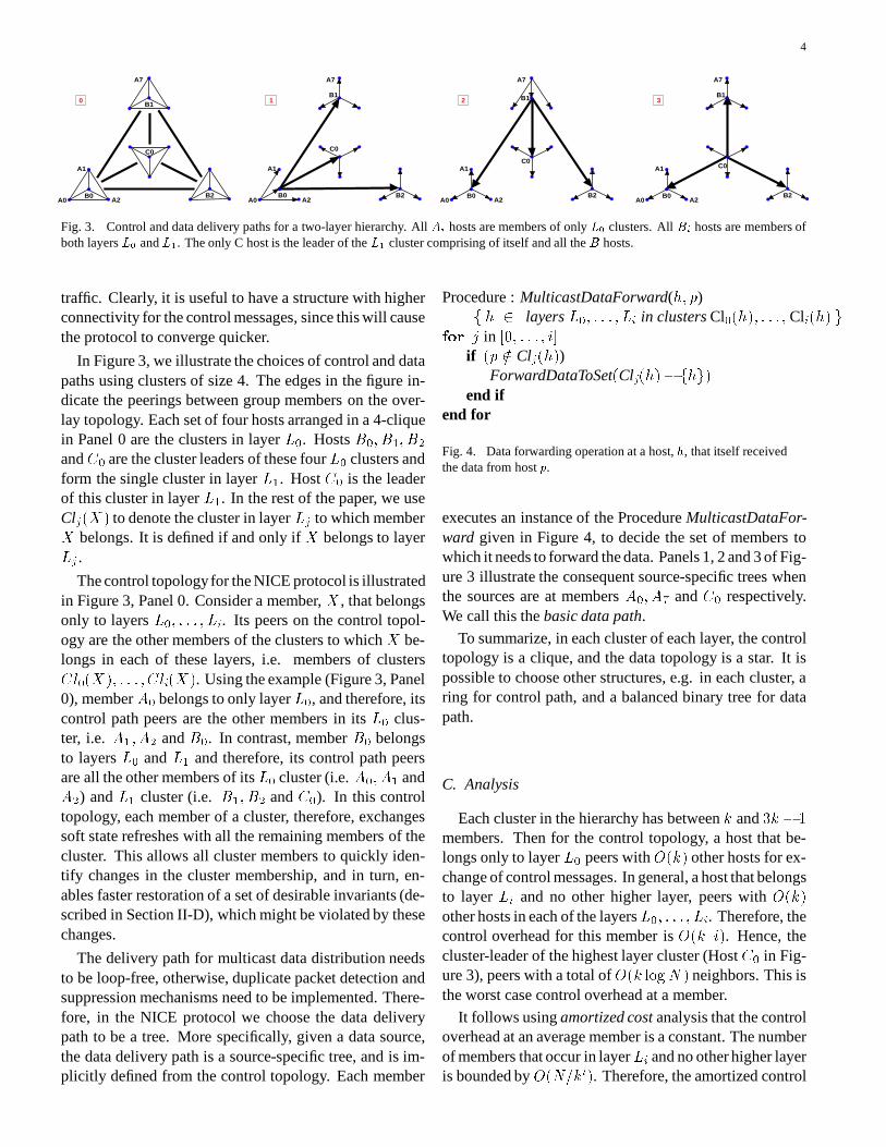
Fig. 3. Control and data delivery paths for a two-layer hierarchy. All Ai hosts are members of only L0 clusters. All Bi hosts are members ofboth layers L0 and L1. The only C host is the leader of the L1 cluster comprising of itself and all the B hosts.

traffic. Clearly, it is useful to have a structure with higherconnectivity for the control messages, since this will causethe protocol to converge quicker.

In Figure 3, we illustrate the choices of control and datapaths using clusters of size 4. The edges in the figure in-dicate the peerings between group members on the over-lay topology. Each set of four hosts arranged in a 4-cliquein Panel 0 are the clusters in layer L0. Hosts B0; B1; B2and C0 are the cluster leaders of these fourL0 clusters andform the single cluster in layer L1. Host C0 is the leaderof this cluster in layer L1. In the rest of the paper, we useClj(X) to denote the cluster in layer Lj to which memberX belongs. It is defined if and only if X belongs to layerLj .

The control topologyfor the NICE protocol is illustratedin Figure 3, Panel 0. Consider a member, X , that belongsonly to layers L0; : : : ; Li. Its peers on the control topol-ogy are the other members of the clusters to which X be-longs in each of these layers, i.e. members of clustersCl0(X); : : : ; Cli(X). Using the example (Figure 3, Panel0), member A0 belongs to only layerL0, and therefore, itscontrol path peers are the other members in its L0 clus-ter, i.e. A1; A2 and B0. In contrast, member B0 belongsto layers L0 and L1 and therefore, its control path peersare all the other members of itsL0 cluster (i.e. A0; A1 andA2) and L1 cluster (i.e. B1; B2 and C0). In this controltopology, each member of a cluster, therefore, exchangessoft state refreshes with all the remaining members of thecluster. This allows all cluster members to quickly iden-tify changes in the cluster membership, and in turn, en-ables faster restoration of a set of desirable invariants (de-scribed in Section II-D), which might be violated by thesechanges.

The delivery path for multicast data distribution needsto be loop-free, otherwise, duplicate packet detection andsuppression mechanisms need to be implemented. There-fore, in the NICE protocol we choose the data deliverypath to be a tree. More specifically, given a data source,the data delivery path is a source-specific tree, and is im-plicitly defined from the control topology. Each member

Procedure : MulticastDataForward(h; p)f h 2 layers L0; : : : ; Li in clusters Cl0(h); : : : ; Cli(h) gfor j in [0; : : : ; i]if (p =2 Clj(h))

ForwardDataToSet(Clj(h)� fhg)end if

end for

Fig. 4. Data forwarding operation at a host, h, that itself receivedthe data from host p.

executes an instance of the Procedure MulticastDataFor-ward given in Figure 4, to decide the set of members towhich it needs to forward the data. Panels 1, 2 and 3 of Fig-ure 3 illustrate the consequent source-specific trees whenthe sources are at members A0; A7 and C0 respectively.We call this the basic data path.

To summarize, in each cluster of each layer, the controltopology is a clique, and the data topology is a star. It ispossible to choose other structures, e.g. in each cluster, aring for control path, and a balanced binary tree for datapath.

C. Analysis

Each cluster in the hierarchy has between k and 3k� 1members. Then for the control topology, a host that be-longs only to layer L0 peers with O(k) other hosts for ex-change of control messages. In general, a host that belongsto layer Li and no other higher layer, peers with O(k)other hosts in each of the layersL0; : : : ; Li. Therefore, thecontrol overhead for this member is O(k i). Hence, thecluster-leader of the highest layer cluster (Host C0 in Fig-ure 3), peers with a total ofO(k logN) neighbors. This isthe worst case control overhead at a member.

It follows using amortized cost analysis that the controloverhead at an average member is a constant. The numberof members that occur in layerLi and no other higher layeris bounded by O(N=ki). Therefore, the amortized control

5

overhead at an average member is� 1N logNXi=0 Nki k:i = O(k) +O( logNN ) +O( 1N )! O(k)with asymptotically increasingN . Thus, the control over-head is O(k) for the average member, and O(k logN) inthe worst case. The same holds analogously for stress atmembers on the basic data path 3. Also, the number ofapplication-level hops on the basic data path between anypair of members is O(logN).

While anO(k logN) peers on the data path is an accept-able upper-bound, we have defined enhancements that fur-ther reduce the upper-bound of the number of peers of amember to a constant. The stress at each member on thisenhanced data path (created using local transformations ofthe basic data path) is thus reduced to a constant, whilethe number of application-level hops between any pair ofmembers still remain bounded by O(logN). We outlinethis enhancement to the basic data path in the Appendix.

D. Invariants

All the properties described in the analysis hold as longas the hierarchy is maintained. Thus, the objective ofNICE protocol is to scalably maintain the host hierarchy asnew members join and existing members depart. Specifi-cally the protocol described in the next section maintainsthe following set of invariants:� At every layer, hosts are partitioned into clusters of

size between k and 3k � 1.� All hosts belong to an L0 cluster, and each host be-longs to only a single cluster at any layer� The cluster leaders are the centers of their respectiveclusters and form the immediate higher layer.

III. PROTOCOL DESCRIPTION

In this section we describe the operations of the NICEprotocol. We assume the existence of a special host thatall members know of a-priori. Using nomenclature devel-oped in [9], we call this host the Rendezvous Point (RP).Each host that intends to join the application-layer multi-cast group contacts the RP to initiate the join process. Forease of exposition, we assume that the RP is always theleader of the single cluster in the highest layer of the hierar-chy. It interacts with other cluster members in this layer onthe control path, and is bypassed on the data path. (Clearly,it is possible for the RP to not be part of the hierarchy, and3Note that the stress metric at members is equivalent to the degree ofthe members on the data delivery tree.

for the leader of the highest layer cluster to maintain a con-nection to the RP, but we do not belabor that complexityfurther). For an application such as streaming media de-livery, the RP could be a distinguished host in the domainof the data source.

The NICE protocol itself has three main components:initial cluster assignment as a new host joins, periodiccluster maintenance and refinement, and recovery fromleader failures. We discuss these in turn.

A. New Host Joins

When a new host joins the multicast group, it must bemapped to some cluster in layer L0. We illustrate the joinprocedure in Figure 5. Assume that hostA12 wants to jointhe multicast group. First, it contacts the RP with its joinquery (Panel 0). The RP responds with the hosts that arepresent in the highest layer of the hierarchy. The joininghost then contacts all members in the highest layer (Panel1) to identify the member closest to itself. In the exam-ple, the highest layer L2 has just one member, C0, whichby default is the closest member to A12 amongst layer L2members. Host C0 informs A12 of the three other mem-bers (B0; B1 and B2) in its L1 cluster. A12 then contactseach of these members with the join query to identify theclosest member among them (Panel 2), and iteratively usesthis procedure to find its L0 cluster.

It is important to note that any host, H , which belongsto any layer Li is the center of its Li�1 cluster, and recur-sively, is an approximation of the center among all mem-bers in allL0 clusters that are below this part of the layeredhierarchy. Hence, querying each layer in succession fromthe top of the hierarchy to layerL0 results in a progressiverefinement by the joining host to find the most appropriatelayer L0 cluster to join that is close to the joining member.The outline of this operation are presented in pseudocodeas Procedure BasicJoinLayer in Figure 6.

We assume that all hosts are aware of only a singlewell-known host, the RP, from which they initiate the joinprocess. Therefore, overheads due to join query-responsemessages is highest at the RP and descreases down thelayers of the hierarchy. Under a very rapid sequence ofjoins, the RP will need to handle a large number of suchjoin query-response messages. Alternate and more scal-able join schemes are possible if we assume that the join-ing host is aware of some other “nearby” host that is al-ready joined to the overlay. In fact, both Pastry [18] andTapestry [22] alleviate a potential bottleneck at the RP fora rapid sequence of joins, based on such an assumption.

1) Join Latency: The joining process involves a mes-sage overhead of O(k logN) query-response pairs. The

6

C0

B0

C0

B0

C0

B0

A12

B1

B2

RP

A12

2B1

B2

RP

0B1

B2

RP

1

A12

Join L0

L2:{ C0 }Join L0

L1: { B0,B1,B2 }

Attach

Fig. 5. Host A12 joins the multicast group.

Procedure : BasicJoinLayer(h; i)Clj Query(RP;�)while (j > i)

Find y s.t. dist(h; y) � dist(h; x); x; y 2 CljClj�1(y) Query(y; j � 1)Decrement j, Clj Clj�1(y)endwhile

JoinCluster(h,Ldr(Clj); Li)Fig. 6. Basic join operation for member h, to join layer Li.i = 0 for a new member. If i > 0, then h is already part oflayer Li�1. Query(y; j � 1) seeks the membership informationof Clj�1(y) from member y. Query(RP;�) seeks the member-ship information of the topmost layer of the hierarchy, from theRP . JoinCluster(x;y; Lj) operation sends an appropriate messageto add new member x to a cluster in layerLj . The message is sentto y, the leader of the cluster.

join-latency depends on the delays incurred in this ex-changes, which is typically about O(logN) round-triptimes. In our protocol, we aggressively locate possible“good” peers for a joining member, and the overhead forlocating the appropriate attachments for any joining mem-ber is relatively large.

To reduce the delay between a member joining the mul-ticast group, and its receipt of the first data packet on theoverlay, we allow joining members to temporarily peer, onthe data path, with the leader of the cluster of the currentlayer it is querying. For example, in Figure 5, when A12is querying the hosts B0; B1 and B2 for the closest pointof attachment, it temporarily peers with C0 (leader of thelayer L1 cluster) on the data path. This allows the joininghost to start receiving multicast data on the group within asingle round-trip latency of its join.

2) Joining Higher Layers: An important invariant inthe hierarchical arrangement of hosts is that the leader ofa cluster be the center of the cluster. Therefore, as mem-bers join and leave clusters, the cluster-leader may occa-sionally change. Consider a change in leadership of a clus-ter, C, in layer Lj . The current leader of C removes itselffrom all layers Lj+1 and higher to which it is attached. A

new leader is chosen for each of these affected clusters.For example, a new leader, h, of C in layer Lj is chosenwhich is now required to join its nearestLj+1 cluster. Thisis its current super-cluster (which by definition is the clus-ter in layer Lj+1 to which the outgoing leader of C wasjoined to), i.e. the new leader replaces the outgoing leaderin the super-cluster. However, if the super-cluster infor-mation is stale and currently invalid, then the new leader,h, invokes the join procedure to join the nearestLj+1 clus-ter. It calls BasicJoinLayer(h; j + 1) and the routine ter-minates when the appropriate layer Lj+1 cluster is found.Also note that the BasicJoinLayer requires interaction ofthe member h with the RP. The RP, therefore, aids in re-pairing the hierarchy from occasional overlay partitions,i.e. if the entire super-cluster information becomes stalein between the periodic HeartBeat messages that are ex-changed between cluster members. If the RP fails, for cor-rect operation of our protocol, we require that it be capableof recovery within a reasonable amount of time.

B. Cluster Maintenance and Refinement

Each member x of a cluster C, sends a HeartBeat mes-sage every � seconds to each of its cluster peers (neighborson the control topology). The message contains the dis-tance estimate of x to each other member ofC. It is possi-ble for x to have inaccurate or no estimate of the distanceto some other members, e.g. immediately after it joins thecluster.

The cluster-leader includes the complete updated clus-ter membership in its HeartBeat messages to all othermembers. This allows existing members to set up appro-priate peer relationships with new cluster members on thecontrol path. For each cluster in levelLi, the cluster-leaderalso periodically sends the its immediate higher layer clus-ter membership (which is the super-cluster for all the othermembers of the cluster) to that Li cluster.

All of the cluster member state is sent via unreliablemessages and is kept by each cluster member as soft-state,refreshed by the periodic HeartBeat messages. A mem-ber x is declared no longer part of a cluster independently

7

Procedure : ClusterSplit(C)f jCj � 3k g� fQjQ � C ^ jQj; jC �Qj � b3k=2cgLet R(Q) � max(radius(Q),radius(C�Q))Find Q� s.t. R(Q�) � R(Q) where Q;Q� 2 �LeaderTransfer(Ldr(C),Q�, Ldr(Q�))LeaderTransfer(Ldr(C),C �Q�, Ldr(C � Q�))Fig. 7. Cluster split operation for cluster, C , which exceedsthe size bound. The operation is invoked by the leader of clus-ter, C . The appropriate partitions (Q� and C � Q�) can benaively implemented in with a running time ofO(jCj3). radius(Q)defines the graph-theoretic radius of the set of members, Q.LeaderTransfer(x;C; y) sends appropriate messages to transfer theleadership of the cluster C from current leader, x, to new leader,y. The LeaderTransfermessage can be sent as a regular HeartBeatmessage with appropriate flags set to indicate the transfer.

Procedure : ClusterMerge(C)f jCj < k and Li is the layer to which C belongs gl Ldr(C)Find y s.t. dist(l; y) < dist(h; x); x; y 2 Cli+1(l)ClusterMergeRequest(l; y; Li)LeaderTransfer(l; C; y)

Fig. 8. Cluster merge operation is invoked by l, the leader of thecluster C . The size of C is < k. l finds y, the leader of anothercluster in layer Li and sends the ClusterMergeRequest message.

by all other members in the cluster if they do not receivea message from x for a configurable number of HeartBeatmessage intervals.

1) Cluster Split and Merge: A cluster-leader periodi-cally checks the size of its cluster, and appropriately splitsor merges the cluster when it detects a size bound viola-tion. A cluster that exceeds the cluster size upper bound,3k � 1 is split into two clusters each of which has at leastb3k=2cmembers. This is described in pseudo-code in Fig-ure 7.

For correct operation of the protocol, we could havechosen the cluster size upper bound to be any value �2k�1. However, if 2k�1was chosen as the upper bound,then the cluster would require to split when it exceeds thisupper bound (i.e. reaches the size 2k). Subsequently, anequal-sized split would create two clusters of size k each.However, a single departure from any of these new clusterswould violate the size lower bound and require a clustermerge operation to be performed. Choosing a larger up-per bound (e.g. 3k-1) avoids this problem. When the clus-ter exceeds this upper bound, it is split into two clusters ofsize at least b3k=2c, and therefore, requires at least dk=2emember departures before a merge operation needs to beinvoked.

Procedure : ClusterRefine(z)f Li is highest layer to which z belongs gl Ldr(Cli(z)); C Cli+1(l)Find y s.t. dist(z; y) < dist(z; x); x; y 2 Cif (y 6= l)

LeaveCluster(z; l; Li)JoinCluster(z; y;Li)endif

Fig. 9. Cluster refine operation by member z which belongs tolayers L0; : : : ; Li and no other higher layer. If it finds another ap-propriate cluster in the same layer, it leaves its current cluster andjoins the other cluster. LeaveCluster(x;y; Lj) sends an appropriatemessage from a departing member x to its cluster leader y in layerLj .

The cluster leader initiates this cluster split operation.Given a set of hosts and the pairwise distances betweenthem, the cluster split operation partitions them into sub-sets that meet the size bounds, such that the maximum ra-dius (in a graph-theoretic sense) of the new set of clus-ters is minimized. This is similar to theK-center problem(known to be NP-Hard) but with an additional size con-straint. We use an approximation strategy — the leadersplits the current cluster into two clusters, each of size atleast b3k=2c, such that the maximum of the radii amongthe two clusters is minimized. It also chooses the centersof the two partitions to be the leaders of the new clustersand transfers leadership to the new leaders through Lead-erTransfer messages. If these new clusters still violate thesize upper bound, they are split by the new leaders usingidentical operations.

If the size of a cluster,C,(in layerLi) with leader l, fallsbelow k, l initiates a cluster merge operation (shown inpseudo-code in Figure 8). Note, l itself belongs to a layerLi+1 cluster, Cli+1(l). l chooses its closest cluster-peer, y,in Cli+1(l). y is also the leader of a layerLi cluster, Cli(y).l initiates the merge operation ofC with Cli(y) by sendinga ClusterMergeRequest message to y. l updates the mem-bers ofC with this merge information. y similarly updatesthe members of Cli(y). Following the merge, l removes it-self from layer Li+1 (i.e. from cluster Cli+1(l).

When a member is joining a layer, it may not always beable to locate the closest cluster in that layer (e.g. due tolost join query or join response, etc.) and instead attachesto some other cluster in that layer. Therefore, each mem-ber, z, in any layer (say Li) periodically probes all mem-bers in its super-cluster (they are the leaders of layer Liclusters), to identify the closest member (say y) to itselfin the super-cluster. If y is not the leader of the Li clus-ter to which z belongs then such an inaccurate attachmentis detected. In this case, z leaves its current layer Li clus-

8

ter and joins the layer Li cluster of which y is the leader.This cluster refinement process is shown in pseudo-codein Figure 9.

C. Host Departure and Leader Selection

When a host x leaves the multicast group, it sends a Re-move message to all clusters to which it is joined. This isa graceful-leave. However, if x fails without being ableto send out this message all cluster peers of x detects thisdeparture through non-receipt of the periodic HeartBeatmessage from x. If x was a leader of a cluster, this trig-gers a new leader selection in the cluster. Each remain-ing member, y, of the cluster independently select a newleader of the cluster, depending on who y estimates to bethe center among these members. Multiple leaders arere-conciled into a single leader of the cluster through ex-change of LeaderTransfer message between the two can-didate leaders, when the multiplicity is detected.

It is possible for members to have an inconsistent viewof the cluster membership, and for transient cycles to de-velop on the data path. These cycles are eliminated oncethe protocol restores the hierarchy invariants and recon-ciles the cluster view for all members.

IV. EXPERIMENTAL METHODOLOGY

We have analyzed the performance of the NICE pro-tocol using detailed simulations and a wide-area imple-mentation. In the simulation environment, we comparethe performance of NICE to three other schemes: multi-unicast, native IP-multicast using the Core Based Tree pro-tocol [2], and the Narada application-layer multicast pro-tocol (as given in [9]). In the Internet experiments, webenchmark the performance metrics against direct unicastpaths to the member hosts.

Clearly, native IP multicast trees will have the least(unit) stress, since each link forwards only a single copyof each data packet. Unicast paths have the lowest la-tency and so we consider them to be of unit stretch 4.They provide us a reference against which to compare theapplication-layer multicast protocols.

A. Data Model

In all these experiments, we model the scenario of a datastream source multicasting to the group. We chose a sin-gle end-host, uniformly at random, to be the data source4There are some recent studies [19], [1] to show that this may notalways be the case; however, we use the native unicast latency as thereference to compare the performance of the other schemes.

generating a constant bit rate data. Each packet in the datasequence, effectively, samples the data path on the over-lay topology at that time instant, and the entire data packetsequence captures the evolution of the data path over time.

B. Performance Metrics

We compare the performance of the different schemesalong the following dimensions:� Quality of data path: This is measured by three dif-

ferent metrics — tree degree distribution, stress onlinks and routers and stretch of data paths to the groupmembers.� Recovery from host failure: As hosts join and leavethe multicast group, the underlying data delivery pathadapts accordingly to reflect these changes. In our ex-periments, we modeled member departures from thegroup as ungraceful departures, i.e. members fail in-stantly and are unable to send appropriate leave mes-sages to their existing peers on the topology. There-fore, in transience, particularly after host failures,path to some hosts may be unavailable. It is also pos-sible for multiple paths to exist to a single host andfor cycles to develop temporarily.To study these effects, we measured the fraction ofhosts that correctly receive the data packets sent fromthe source as the group membership changed. Wealso recorded the number of duplicates at each host.In all of our simulations, for both the application-layer multicast protocols, the number of duplicateswas insignificant and zero in most cases.� Control traffic overhead: We report the mean, vari-ance and the distribution of the control bandwidthoverheads at both routers and end hosts.

V. SIMULATION EXPERIMENTS

We have implemented a packet-level simulator for thefour different protocols. Our network topologies weregenerated using the Transit-Stub graph model, using theGT-ITM topology generator [4]. All topologies in thesesimulations had 10; 000 routers with an average node de-gree between 3 and 4. End-hosts were attached to a setof routers, chosen uniformly at random, from among thestub-domain nodes. The number of such hosts in the mul-ticast group were varied between 8 and 2048 for differentexperiments. In our simulations, we only modeled loss-less links; thus, there is no data loss due to congestion, andno notion of background traffic or jitter. However, datais lost whenever the application-layer multicast protocol

9

fails to provide a path from the source to a receiver, andduplicates are received whenever there is more than onepath. Thus, our simulationsstudy the dynamics of the mul-ticast protocol and its effects on data distribution; in ourimplementation, the performance is also affected by otherfactors such as additional link latencies due to congestionand drops due to cross-traffic congestion.

A. Our implementation of Narada

We have implemented the entire Narada protocol fromthe description given in [9]. We did not implement theNarada high bandwidth extensions described in [8].As de-scribed before, Narada is a mesh-first application-layermulticast approach, designed primarily for small multicastgroups. In Narada, the initial set of peer assignments tocreate the overlay topology is done randomly. While thisinitial data delivery path may be of “poor” quality, overtime Narada adds “good” links and discards “bad” linksfrom the overlay. Narada has O(N2) aggregate controloverhead because of its mesh-first nature: it requires eachhost to periodically exchange updates and refreshes withall other hosts.

The protocol, as defined in [9], has a number of user-defined parameters that we needed to set. These includethe link add/drop thresholds, link add/drop probe fre-quency, the periodic refresh rates, the mesh degree, etc.We experimented with a wide-range of values for theseparameters to understand the behavior of Narada and ob-served some interesting trade-offs in choosing these pa-rameters. Specifically, we found that:� The mesh degree bound for hosts should not be

strictly enforced to ensure connectivity. Instead ad-ditional mechanisms that limit the degree of the datapath on the mesh should be used.� There is a clear tradeoff between choosing a high ver-sus low frequency for periodic probes to add or droplinks on the mesh. A high frequency allows mem-bers to aggressively add and drop good and bad over-lay links respectively. However, this leads to frequentchanges to the data paths on the mesh, which can leadto a temporary loss of data path to other members.(This effect is different than when a route changes andstate for the old route can be temporarily maintainedto mitigate the effect of the route change). We ob-served this effect in our experiments where we use ahigh periodic probe frequency, especially if this pa-rameter is set higher than the route packet exchangefrequency. In contrast, using a low probe frequencyleads to more stable paths; however, this implies thatthe mesh topology takes a long time to stabilize.

B. Simulation Results

We have simulated a wide-range of topologies, groupsizes, member join-leave patterns, and protocol parame-ters. For NICE, we set the cluster size parameter, k, to 3in all of the experiments presented here. Broadly, our find-ings can be summarized as follows:� NICE trees have data paths that have stretch compa-

rable to Narada.� The stress on links and routers are lower in NICE, es-pecially as the multicast group size increases.� The failure recovery of both the schemes are compa-rable.� NICE protocol demonstrates that it is possible toprovide these performance with orders of magnitudelower control overhead for groups of size > 32.

We begin with results from a representative experimentthat captures all the of different aspects comparing the var-ious protocols.

1) Simulation Representative Scenario: This experi-ment has two different phases: a join phase and a leavephase. In the join phase a set of 128 members5 join themulticast group uniformly at random between the simu-lated time 0 and 200 seconds. These hosts are allowed tostabilize into an appropriate overlay topology until simu-lation time 1000 seconds. The leave phase starts at time1000 seconds: 16 hosts leave the multicast group over ashort duration of 10 seconds. This is repeated four moretimes, at 100 second intervals. The remaining 48 mem-bers continue to be part of the multicast group until theend of simulation. All member departures are modeled ashost failures since they have the most damaging effect ondata paths. We experimented with different numbers ofmember departures, from a single member to 16 membersleaving over the ten second window. Sixteen departuresfrom a group of size 128 within a short time window isa drastic scenario, but it helps illustrate the failure recov-ery modes of the different protocols better. Member de-partures in smaller sizes cause correspondingly lower dis-ruption on the data paths.

We experimented with different periodic refresh ratesfor Narada. For a higher refresh rate the recovery fromhost failures is quicker, but at a cost of higher controltraffic overhead. For Narada, we used different valuesfor route update frequencies and periods for probing othermesh members to add or drop links on the overlay. In our5We show results for the 128 member case because that is the groupsize used in the experiments reported in [9]; NICE performs increas-ingly better with larger group sizes.

10

1.3

1.4

1.5

1.6

1.7

1.8

1.9

2

2.1

2.2

2.3

100 200 300 400 500 600 700 800 900

Ave

rage

link

str

ess

Time (in secs)

128 end-hosts join

128Join Narada-5

NICE

Fig. 10. Average link stress (simulation)

10

15

20

25

30

100 200 300 400 500 600 700 800 900

Ave

rage

rec

eive

r pa

th le

ngth

(ho

ps)

Time (in secs)

128 end-hosts join

128Join

Narada-5NICEIP MulticastUnicast

Fig. 11. Average path length (simulation)

results, we report results from using route update frequen-cies of once every 5 seconds (labeled Narada-5), and onceevery 30 seconds (labeled Narada-30). The 30 second up-date period corresponds to the what was used in [9]; we ranwith the 5 second update period since the heartbeat periodin NICE was set to 5 seconds. Note that we could run witha much smaller heartbeat period in NICE without signifi-cantly increasing control overhead since the control mes-sages are limited within clusters and do not traverse the en-tire group. We also varied the mesh probe period in Naradaand observed data path instability effect discussed above.In these results, we set the Narada mesh probe period to 20seconds.

Data Path Quality: In Figures 10 and 11, we show theaverage link stress and the average path lengths for the dif-ferent protocols as the data tree evolves during the mem-ber join phase. Note that the figure shows the actual pathlengths to the end-hosts; the stretch is the ratio of averagepath length of the members of a protocol to the averagepath length of the members in the multi-unicast protocol.

As explained earlier, the join procedure in NICE aggres-sively finds good points of attachment for the members inthe overlay topology, and the NICE tree converges quickerto a stable value (within 350 seconds of simulated time).In contrast, the Narada protocols gradually improve themesh quality, and consequently so does the data path overa longer duration. Its average data path length convergesto a stable value of about 23 hops between 500 and 600seconds of the simulated time. The corresponding stretchis about 2.18. In Narada path lengths improve over timedue to addition of “good” links on the mesh. At the sametime, the stress on the tree gradually increases since theNarada decides to add or drop overlay links based purelyon the stretch metric.

The cluster-based data dissemination in NICE reduces

average link stress, and in general, for large groups NICEconverges to trees with about 25% lower average stress.In this experiment, the NICE tree had lower stretch thanthe Narada tree; however, in other experiments the Naradatree had a slightly lower stretch value. In general, com-paring the results from multiple experiments over differ-ent group sizes, (See Section V-B.2), we concluded thatthe data path lengths to receivers were similar for both pro-tocols.

In Figures 12 and 13, we plot a cumulative distributionof the stress and path length metrics for the entire mem-ber set (128 members) at a time after the data paths haveconverged to a stable operating point.

The distribution of stress on links for the multi-unicastscheme has a significantly large tail (e.g. links close tothe source has a stress of 127). This should be contrastedwith better stress distribution for both NICE and Narada.Narada uses fewer number of links on the topology thanNICE, since it is comparably more aggressive in addingoverlay links with shorter lengths to the mesh topology.However, due to this emphasis on shorter path lengths, thestress distributionof the links has a heavier-tail than NICE.More than 25% of the links have a stress of four and higherin Narada, compared to< 5% in NICE. The distribution ofthe path lengths for the two protocols are comparable.

Failure Recovery and Control Overheads: To investi-gate the effect of host failures, we present results fromthe second part of our scenario: starting at simulated time1000 seconds, a set of 16 members leave the group overa 10 second period. We repeat this procedure four moretimes and no members leave after simulated time 1400 sec-onds when the group is reduced to 48 members. Whenmembers leave, both protocols “heal” the data distribu-tion tree and continue to send data on the partially con-nected topology. In Figure 14, we show the fraction of

11

0

100

200

300

400

500

600

0 5 10 15 20 25 30 35

Num

ber

of li

nks

Link stress

Cumulative distribution of link stress after overlay stabilizes

(Unicast truncatedExtends to stress = 127)

NICENarada-5

Unicast

Fig. 12. Stress distribution (simulation)

0

20

40

60

80

100

120

5 10 15 20 25 30 35 40

Num

ber

of h

osts

Overlay path length (hops)

Cumulative distribution of data path lengths after overlay stabilizes

UnicastIP Multicast

NICENarada-5

Fig. 13. Path length distribution (simulation)

members that correctly receive the data packets over thisduration. Both Narada-5 and NICE have similar perfor-mance, and on average, both protocols restore the datapath to all (remaining) receivers within 30 seconds. Wealso ran the same experiment with the 30 second refreshperiod for Narada. The lower refresh period caused signif-icant disruptions on the tree with periods of over 100 sec-onds when more than 60% of the tree did not receive anydata. Lastly, we note that the data distribution tree used forNICE is the least connected topology possible; we expectfailure recovery results to be much better if structures withalternate paths are built atop NICE.

In Figure 15, we show the byte-overheads for controltraffic at the access links of the end-hosts. Each dot in theplot represents the sum of the control traffic (in Kbps) sentor received by each member in the group, averaged over 10second intervals. Thus for each 10 second time slot, thereare two dots in the plot for each (remaining) host in themulticast group corresponding to the control overheads forNarada and NICE. The curves in the plot are the averagecontrol overhead for each protocol. As can be expected,for groups of size 128, NICE has an order of magnitudelower average overhead, e.g. at simulation time 1000 sec-onds, the average control overhead for NICE is 0.97 Kbpsversus 62.05 Kbps for Narada. At the same time instant,Narada-30 (not shown in the figure) had an average con-trol overhead of 13.43 Kbps. Note that the NICE controltraffic includes all protocol messages, including messagesfor cluster formation, cluster splits, merges, layer promo-tions, and leader elections.

2) Aggregate Results: We present a set of aggregateresults as the group size is varied. The purpose of thisexperiment is to understand the scalability of the differ-ent application-layer multicast protocols. The entire setof members join in the first 200 seconds, and then we run

the simulation for 1800 seconds to allow the topologies tostabilize. In Table I, we compare the stress on networkrouters and links, the overlay path lengths to group mem-bers and the average control traffic overheads at the net-work routers. For each metric, we present the both meanand the standard deviation. Note, that the Narada protocolinvolves an aggregate control overhead of O(N2), whereN is the size of the group. Therefore, in our simulationsetup, we were unable to simulate Narada with groups ofsize 1024 or larger since the completion time for these sim-ulations were on the order of a day for a single run of oneexperiment on a 550 MHz Pentium III machine with 4 GBof RAM.

Narada and NICE tend to converge to trees with similarpath lengths. The stress metric for both network links androuters, however, is consistently lower for NICE when thegroup size is large (64 and greater). It is interesting to ob-serve the standard deviation of stress as it changes with in-creasing group size for the two protocols. The standard de-viation for stress increased for Narada for increasing groupsizes. In contrast, the standard deviation of stress for NICEremains relatively constant; the topology-based clusteringin NICE distributes the data path more evenly among thedifferent links on the underlying links regardless of groupsize.

The control overhead numbers in the table are differ-ent than the ones in Figure 15; the column in the table isthe average control traffic per network router as opposedto control traffic at an end-host. Since the control trafficgets aggregated inside the network, the overhead at routersis significantly higher than the overhead at an end-host.For these router overheads, we report the values of theNarada-30 version in which the route update frequency setto 30 seconds. Recall that the Narada-30 version has poorfailure recovery performance, but is much more efficient

12

0.5

0.6

0.7

0.8

0.9

1

1000 1100 1200 1300 1400 1500 1600

Fra

ctio

n of

hos

ts th

at c

orre

ctly

rec

eive

d da

ta

Time (in secs)

128 end-hosts join followed by periodic leaves in sets of 16

16 X 5Leave

NICENarada-5

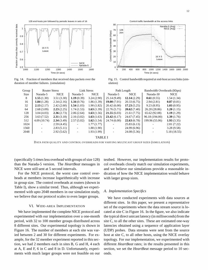
Fig. 14. Fraction of members that received data packets over theduration of member failures. (simulation)

0

10

20

30

40

50

60

70

80

0 200 400 600 800 1000 1200 1400 1600 1800 2000

Con

trol

traf

fic b

andw

idth

(K

bps)

Time (in secs)

Control traffic bandwidth at the access links

128Join

16 X 5Leave

Narada-5 (Avg)NICE (Avg)

Fig. 15. Control bandwidth required at end-host access links (sim-ulation)

Group Router Stress Link Stress Path Length Bandwidth Overheads (Kbps)Size Narada-5 NICE Narada-5 NICE Narada-5 NICE Narada-30 NICE

8 1.55 (1.30) 3.51 (3.30) 1.19 (0.39) 3.24 (2.90) 25.14 (9.49) 12.14 (2.29) 0.61 (0.55) 1.54 (1.34)16 1.84 (1.28) 2.34 (2.16) 1.34 (0.76) 1.86 (1.39) 19.00 (7.01) 20.33 (6.75) 2.94 (2.81) 0.87 (0.81)32 2.13 (2.17) 2.42 (2.60) 1.54 (1.03) 1.90 (1.82) 20.42 (6.00) 17.23 (5.25) 9.23 (8.95) 1.03 (0.95)64 2.68 (3.09) 2.23 (2.25) 1.74 (1.53) 1.63 (1.39) 22.76 (5.71) 20.62 (7.40) 26.20 (28.86) 1.20 (1.15)128 3.04 (4.03) 2.36 (2.73) 2.06 (2.64) 1.63 (1.56) 21.55 (6.03) 21.61 (7.75) 65.62 (92.08) 1.19 (1.29)256 3.63 (7.52) 2.31 (3.18) 2.16 (3.02) 1.63 (1.63) 23.42 (6.17) 24.67 (7.45) 96.18 (194.00) 1.39 (1.76)512 4.09 (10.74) 2.34 (3.49) 2.57 (5.02) 1.62 (1.54) 24.74 (6.00) 22.63 (6.78) 199.96 (55.06) 1.93 (3.35)1024 - 2.59 (4.45) - 1.77 (1.77) - 25.83 (6.13) - 2.81 (7.22)1560 - 2.83 (5.11) - 1.88 (1.90) - 24.99 (6.96) - 3.28 (9.58)2048 - 2.92 (5.62) - 1.93 (1.99) - 24.08 (5.36) - 5.18 (18.55)

TABLE IDATA PATH QUALITY AND CONTROL OVERHEADS FOR VARYING MULTICAST GROUP SIZES (SIMULATION)

(specifically 5 times less overhead with groups of size 128)than the Narada-5 version. The HeartBeat messages inNICE were still sent at 5 second intervals.

For the NICE protocol, the worst case control over-heads at members increase logarithmically with increasein group size. The control overheads at routers (shown inTable I), show a similar trend. Thus, although we experi-mented with upto 2048 members in our simulation study,we believe that our protocol scales to even larger groups.

VI. WIDE-AREA IMPLEMENTATION

We have implemented the complete NICE protocol andexperimented with our implementation over a one-monthperiod, with 32 to 100 member groups distributed across8 different sites. Our experimental topology is shown inFigure 16. The number of members at each site was var-ied between 2 and 30 for different experiments. For ex-ample, for the 32 member experiment reported in this sec-tion, we had 2 members each in sites B, G and H, 4 eachat A, E and F, 6 in C and 8 in D. Unfortunately, experi-ments with much larger groups were not feasible on our

testbed. However, our implementation results for proto-col overheads closely match our simulation experiments,and we believe our simulations provide a reasonable in-dication of how the NICE implementation would behavewith larger group sizes.

A. Implementation Specifics

We have conducted experiments with data sources atdifferent sites. In this paper, we present a representativeset of the experiments where the data stream source is lo-cated at site C in Figure 16. In the figure, we also indicatethe typical direct unicast latency (in milliseconds) from thesite C, to all the other sites. These are estimated one-waylatencies obtained using a sequence of application layer(UDP) probes. Data streams were sent from the sourcehost at site C, to all other hosts, using the NICE overlaytopology. For our implementation, we experimented withdifferent HeartBeat rates; in the results presented in thissection, we set the HeartBeat message period to 10 sec-onds.

13

G

H

F

E

DC

B

A

39.4

35.5

4.6

0.6

0.5

1.7

33.3

Source

A: cs.ucsb.edu

B: asu.edu

C: cs.umd.edu

D: glue.umd.edu

E: wam.umd.edu

F: umbc.edu

G: poly.edu

H: ecs.umass.edu

Fig. 16. Internet experiment sites and direct unicast latencies from C

In our implementation, we had to estimate the end-to-end latency between hosts for various protocol operations,including member joins, leadership changes, etc. We es-timated the latency between two end-hosts using a low-overhead estimator that sent a sequence of application-layer (UDP) probes. We controlled the number of probesadaptively using observed variance in the latency esti-mates. Further, instead of using the raw latency estimatesas the distance metric, we used a simple binning scheme tomap the raw latencies to a small set of equivalence classes.Specifically, two latency estimates were considered equiv-alent if they mapped to the same equivalence class, andthis resulted in faster convergence of the overlay topology.The specific latency ranges for each class were 0-1 ms, 1-5ms, 5-10 ms, 10-20 ms, 20-40 ms, 40-100 ms, 100-200 msand greater than 200 ms.

To compute the stretch for end-hosts in the Internet ex-periments, we used the ratio of the latency from betweenthe source and a host along the overlay to the direct uni-cast latency to that host. In the wide-area implementa-tion, when a host A receives a data packet forwarded bymember B along the overlay tree, A immediately sendsback a overlay-hop acknowledgment back to B. B logsthe round-trip latency between its initial transmission ofthe data packet toA and the receipt of the acknowledgmentfromA. After the entire experiment is done, we calculatedthe overlay round-trip latencies for each data packet byadding up the individual overlay-hop latencies availablefrom the logs at each host. We estimated the one-way over-lay latency as half of this round trip latency. We obtainedthe unicast latencies using our low-overhead estimator im-mediately after the overlay experiment terminated. Thisguaranteed that the measurements of the overlay latenciesand the unicast latencies did not interfere with each other.

0.7

0.75

0.8

0.85

0.9

0.95

1

1 2 3 4 5 6 7 8 9

Fra

ctio

n of

mem

bers

Stress

Cumulative distribution of stress

32 members64 members96 members

Fig. 17. Stress distribution (testbed)

B. Implementation Scenarios

The Internet experiment scenarios have two phases: ajoin phase and a rapid membership change phase. In thejoin phase, a set of member hosts randomly join the groupfrom the different sites. The hosts are then allowed to sta-bilize into an appropriate overlay delivery tree. After thisperiod, the rapid membership change phase starts, wherehost members randomly join and leave the group. The av-erage member lifetime in the group, in this phase was setto 30 seconds. Like in the simulation studies, all memberdepartures are ungraceful and allow us to study the worstcase protocol behavior. Finally, we let the remaining set ofmembers to organize into a stable data delivery tree. Wepresent results for three different groups of size of 32, 64,and 96 members.

Data Path Quality

In Figure 17, we show the cumulative distributionof thestress metric at the group members after the overlay stabi-lizes at the end of the join phase. For all group sizes, typ-ical members have unit stress (74% to 83% of the mem-bers in these experiments). The stress for the remainingmembers vary between 3 and 9. These members are pre-cisely the cluster leaders in the different layers (recall thatthe cluster size lower and upper bounds for these experi-ments is 3 and 9, respectively). The stress for these mem-bers can be reduced further by using the high-bandwidthdata path enhancements, described in the Appendix. Forlarger groups, the number of members with higher stress(i.e. between 3 and 9 in these experiments) is more, sincethe number of clusters (and hence, the number of clusterleaders) is more. However, as expected, this increase isonly logarithmic in the group size.

In Figure 18, we plot the cumulative distribution of thestretch metric. Instead of plotting the stretch value for each

14

1

2

3

4

5

6

7

8

9

A B C D E F G H

Str

etch

Sites

Distribution of stretch (64 members)

Fig. 18. Stretch distribution (testbed)

0

5

10

15

20

25

30

35

40

45

A B C D E F G H

Ove

rlay

end-

to-e

nd la

tenc

y (in

ms)

Sites

Distribution of latency (64 members)

Fig. 19. Latency distribution (testbed)

single host, we group them by the sites at which there arelocated. For all the member hosts at a given site, we plotthe mean and the 95% confidence intervals. Apart fromthe sites C, D, and E, all the sites have near unit stretch.However, note that the source of the data streams in theseexperiments were located in site C and hosts in the sites C,D, and E had very low latency paths from the source host.The actual end-to-end latencies along the overlay paths toall the sites are shown in Figure 19. For the sites C, D andE these latencies were 3.5 ms, 3.5 ms and 3.0 ms respec-tively. Therefore, the primary contribution to these laten-cies are packet processing and overlay forwarding on theend-hosts themselves.

In Table II, we present the mean and the maximumstretch for the different members, that had direct unicastlatency of at least 2 ms from the source (i.e. sites A, B, Gand H), for all the different sizes. The mean stretch for allthese sites are low. However, in some cases we do see rela-tively large worst case stretches (e.g. in the 96-member ex-periment there was one member that for which the stretchof the overlay path was 4.63).

0.4

0.5

0.6

0.7

0.8

0.9

1

0 100 200 300 400 500 600 700 800 900

Fra

ctio

n of

hos

ts th

at c

orre

ctly

rec

eive

dat

a

Time (in secs)

Distribution of losses for packets in random membership change phase

64 membersAverage member lifetime = 30 secs

Fig. 20. Fraction of members that received data packets as groupmembership continuously changed (testbed)

0

0.1

0.2

0.3

0.4

0.5

0.6

0.7

0.8

0.9

1

0 0.01 0.02 0.03 0.04 0.05

Fra

ctio

n of

mem

bers

Fraction of packets lost

Cumulative distribution of losses at members in random membership change phase

Fig. 21. Cumulative distribution of fraction of packets lost for dif-ferent members out of the entire sequenceof 900 packets during therapid membership change phase (testbed)

Failure Recovery

In this section, we describe the effects of group mem-bership changes on the data delivery tree. To do this, weobserve how successful the overlay is in delivering dataduring changes to the overlay topology. We measured thenumber of correctly received packets by different (remain-ing) members during the rapid membership change phaseof the experiment, which begins after the initial memberset has stabilized into the appropriate overlay topology.This phase lasts for 15 minutes. Members join and leavethe grou at random such that the average lifetime of amember in the group is 30 seconds.

In Figure 20 we plot over time the fraction of mem-bers that successfully received the different data packets.A total of 30 group membership changes happened overthe duration. In Figure 21 we plot the cumulative dis-tribution of packet losses seen by the different membersover the entire 15 minute duration. The maximum num-ber of packet losses seen by a member was 50 out of 900(i.e. about 5.6%), and 30% of the members did not en-

15

Group Stress Stretch Control overheads (Kbps)Size Mean Max. Mean Max. Mean Max.32 1.85 8.0 1.08 1.61 0.84 2.3464 1.73 8.0 1.14 1.67 0.77 2.7096 1.86 9.0 1.04 4.63 0.73 2.65

TABLE IIAVERAGE AND MAXIMUM VALUES OF OF THE DIFFERENT

METRICS FOR DIFFERENT GROUP SIZES(TESTBED)

counter any packet losses. Even under this rapid changesto the group membership, the largest continuous durationof packet losses for any single host was 34 seconds, whiletypical members experienced a maximum continuous dataloss for only two seconds — this was true for all but 4 ofthe members. These failure recovery statistics are goodenough for use in most data stream applications deployedover the Internet. Note that in this experiment, only threeindividual packets (out of 900) suffered heavy losses: datapackets at times 76 s, 620 s, and 819 s were not receivedby 51, 36 and 31 members respectively.

Control Overheads

Finally, we present the control traffic overheads (inKbps) in Table II for the different group sizes. The over-heads include control packets that were sent as well as re-ceived. We show the average and maximum control over-head at any member. We observed that the control trafficat most members lies between 0.2 Kbps to 2.0 Kbps forthe different group sizes. In fact, about 80% of the mem-bers require less than 0.9 Kbps of control traffic for topol-ogy management. More interestingly, the average controloverheads and the distributionsdo not change significantlyas the group size is varied. The worst case control over-head is also fairly low (less than 3 Kbps).

VII. RELATED WORK

A number of other projects have explored implementingmulticast at the application layer. They can be classifiedinto two broad categories: mesh-first (Narada [9], Gos-samer [6]) and tree-first protocols (Yoid [11], ALMI [14],Host-Multicast [21]). Yoid and Host-Multicast defines adistributed tree building protocol between the end-hosts,while ALMI uses a centralized algorithm to create a mini-mum spanning tree rooted at a designated single source ofmulticast data distribution. The Overcast protocol [13] or-ganizes a set of proxies (called Overcast nodes) into a dis-tribution tree rooted at a central source for single sourcemulticast. A distributed tree-building protocol is used tocreate this source specific tree, in a manner similar to Yoid.

RMX [7] provides support for reliable multicast data de-livery to end-hosts using a set of similar proxies, called Re-liable Multicast proXies. Application end-hosts are con-figured to affiliate themselves with the nearest RMX. Thearchitecture assumes the existence of an overlay construc-tion protocol, using which these proxies organize them-selves into an appropriate data delivery path. TCP is usedto provide reliable communication between each pair ofpeer proxies on the overlay.

Some other recent projects (Chord [20], Content Ad-dressable Networks (CAN) [16], Tapestry [22] and Pas-try [18]) have also addressed the scalability issue in cre-ating application layer overlays, and are therefore, closelyrelated to our work. CAN defines a virtual d-dimensionalCartesian coordinate space, and each overlay host “owns”a part of this space. In [17], the authors have leveragedthe scalable structure of CAN to define an applicationlayer multicast scheme, in which hosts maintainO(d) stateand the path lengths are O(dN1=d) application level hops,whereN is the number of hosts in the network. Pastry [18]is a self-organizing overlay network of nodes, where log-ical peer relationships on the overlay are based on match-ing prefixes of the node identifiers. Scribe [5] is a large-scale event notification infrastructure that leverages thePastry system to create groups and build efficient applica-tion layer multicast paths to the group members for dis-semination of events. Being based on Pastry, it has sim-ilar overlay properties, namely (2b � 1) log2b N state atmembers, andO(log2b N) application level hops betweenmembers 6. Bayeux [23] in another architecture for ap-plication layer multicast, where the end-hosts are orga-nized into a hierarchy as defined by the Tapestry over-lay location and routing system [22]. A level of the hi-erarchy is defined by a set of hosts that share a commonsuffix in their host IDs. Such a technique was proposedby Plaxton et.al. [15] for locating and routing to namedobjects in a network. Therefore, hosts in Bayeux main-tain O(b logbN) state and end-to-end overlay paths haveO(logbN) application level hops. As discussed in Sec-tion II-C, our proposed NICE protocol incurs an amor-tized O(k) state at members and the end-to-end paths be-tween members have O(logkN) application level hops.Like Pastry and Tapestry, NICE also chooses overlay peersbased on network locality which leads to low stretch end-to-end paths.

We summarize the above as follows: For both NICE andCAN-multicast, members maintain constant state for othermembers, and consequently exchange a constant amountof periodic refreshes messages. This overhead is loga-rithmic for Scribe and Bayeux. The overlay paths for6b is a small constant.

16

NICE, Scribe, and Bayeux have a logarithmic number ofapplication level hops, and path lengths in CAN-multicastasymptotically have a larger number of application levelhops. Both NICE and CAN-multicast use a single well-known host (the RP, in our nomenclature) to bootstrap thejoin procedure of members. The join procedure, there-fore, incurs a higher overhead at the RP and the higherlayers of the hierarchy than the lower layers. Scribe andBayeux assume members are able find different “nearby”members on the overlay through out-of-band mechanisms,from which to bootstrap the join procedure. Using this as-sumption, the join overheads for a large number of join-ing members can be amortized over the different such“nearby” bootstrap members in these schemes.

VIII. CONCLUSIONS

In this paper, we have presented a new protocol forapplication-layer multicast. Our main contribution is anextremely low overhead hierarchical control structure overwhich different data distribution paths can be built. Ourresults show that it is possible to build and maintainapplication-layer multicast trees with very little overhead.While the focus of this paper has been low-bandwidth datastream applications, our scheme is generalizable to differ-ent applications by appropriately choosing data paths andmetrics used to construct the overlays. We believe that theresults of this paper are a significant first step towards con-structing large wide-area applications over application-layer multicast.

IX. ACKNOWLEDGMENTS

Srinivas Parthasarathy implemented a part of theNarada protocol used in our simulation experiments.We thank Kevin Almeroth, Lixin Gao, Jorg Liebeherr,Steven Low, Martin Reisslein and Malathi Veeraraghavanfor providing us with user accounts at the different sitesfor our wide-area experiments and Peter Druschel forproviding many useful comments on a previous versionof this paper.

REFERENCES

[1] D. Andersen, H. Balakrishnan, M. Frans Kaashoek, and R. Mor-ris. Resilient overlay networks. In Proceedingsof 18th ACM Sym-posium on Operating Systems Principles, Oct. 2001.

[2] T. Ballardie, P. Francis, and J. Crowcroft. Core Based Trees(CBT): An Architecture for Scalable Multicast Routing. In Pro-ceedings of ACM Sigcomm, 1995.

[3] S. Banerjee and B. Bhattacharjee. Scalable Secure Group Com-munication over IP Mulitcast. In Proceedingsof Internation Con-ference on Network Protocols, Nov. 2001.

[4] K. Calvert, E. Zegura, and S. Bhattacharjee. How to Model anInternetwork. In Proceedings of IEEE Infocom, 1996.

[5] M. Castro, P. Druschel, A.-M. Kermarrec, and A. Rowstron.SCRIBE: A large-scale and decentralized application-level mul-ticast infrastructure. IEEE Journal on Selected Areas in commu-nications (JSAC), 2002. To appear.

[6] Y. Chawathe. Scattercast: An Architecture for Internet BroadcastDistribution as an Infrastructure Service. Ph.D. Thesis, Univer-sity of California, Berkeley, Dec. 2000.

[7] Y. Chawathe, S. McCanne, and E. A. Brewer. RMX: ReliableMulticast for Heterogeneous Networks. In Proceedings of IEEEInfocom, 2000.

[8] Y.-H. Chu, S. G. Rao, S. Seshan, and H. Zhang. Enabling Con-ferencing Applications on the Internet using an Overlay MulticastArchitecture. In Proceedings of ACM SIGCOMM, Aug. 2001.

[9] Y.-H. Chu, S. G. Rao, and H. Zhang. A Case for End SystemMulticast. In Proceedings of ACM SIGMETRICS, June 2000.

[10] S. Deering and D. Cheriton. Multicast Routing in Datagram In-ternetworks and Extended LANs. In ACM Transactions on Com-puter Systems, May 1990.

[11] P. Francis. Yoid: Extending the Multicast Internet Architecture,1999. White paper http://www.aciri.org/yoid/.

[12] A. Gupta. Steiner points in tree metrics don’t (really) help. InSymposium of Discrete Algorithms, Jan. 2001.

[13] J. Jannotti, D. Gifford, K. Johnson, M. Kaashoek, and J. O’Toole.Overcast: Reliable Multicasting with an Overlay Network. InProceedings of the 4th Symposium on Operating Systems Designand Implementation, Oct. 2000.

[14] D. Pendarakis, S. Shi, D. Verma, and M. Waldvogel. ALMI: AnApplication Level Multicast Infrastructure. In Proceedingsof 3rdUsenix Symposium on Internet Technologies & Systems, March2001.

[15] C. G. Plaxton, R. Rajaraman, and A. W. Richa. Accessing nearbycopies of replicated objects in a distributed environment. In ACMSymposium on Parallel Algorithms and Architectures, June 1997.

[16] S. Ratnasamy, P. Francis, M. Handley, R. Karp, and S. Shenker.A scalable content-addressable network. In Proceedings of ACMSigcomm, Aug. 2001.

[17] S. Ratnasamy,M. Handley, R. Karp, and S. Shenker. Application-level multicast using content-addressable networks. In Proceed-ings of 3rd InternationalWorkshopon NetworkedGroup Commu-nication, Nov. 2001.

[18] A. Rowstron and P. Druschel. Pastry: Scalable, distributed ob-ject location and routing for large-scale peer-to-peer systems.In IFIP/ACM International Conference on Distributed SystemsPlatforms (Middleware), Nov. 2001.

[19] S. Savage, T. Anderson, A. Aggarwal, D. Becker, N. Cardwell,A. Collins, E. Hoffman, J. Snell, A. Vahdat, G. Voelker, and J. Za-horjan. Detour: A Case for Informed Internet Routing and Trans-port. IEEE Micro, 19(1), Jan. 1999.

[20] I. Stoica, R. Morris, D. Karger, M. F. Kaashoek, andH.Balakrishnan. Chord: A scalable peer-to-peer lookupservice for Internet applications. In Proceedings of ACMSigcomm, Aug. 2001.

[21] B. Zhang, S. Jamin, and L. Zhang. Host multicast: A frameworkfor delivering multicast to end users. In Proceedings of IEEE In-focom, June 2002.

[22] B. Y. Zhao, J. Kubiatowicz, and A. Joseph. Tapestry: An In-frastructure for Fault-tolerant Wide-area Location and Routing.Technical report, UCB/CSD-01-1141, University of California,Berkeley, CA, USA, Apr. 2001.

[23] S. Q. Zhuang,B. Y. Zhao, A. D. Joseph,R. Katz, and J. Kubiatow-icz. Bayeux: An architecture for scalable and fault-tolerant wide-area data dissemination. In Eleventh International Workshop on

17

B0 B2

B1

C0

B0 B2

B13

A2

C0

A4

A6

A2

A6

A4 A5

A3

A5

A3A10

4

A10

Fig. 22. Data path enhancements using delegation.

Network and Operating Systems Support for Digital Audio andVideo (NOSSDAV 2001), 2001.

APPENDIX

DATA PATH ENHANCEMENTS FOR HIGH BANDWIDTH

APPLICATIONS

The basic data path in NICE imposes more data for-warding responsibility onto the cluster leaders. As a con-sequence, members that are joined to higher layers arecluster leaders in all the lower layers that they are joined to.Therefore, they are required to forward higher volume ofdata than those members that are joined to only the lowerlayers. This data forwarding path, is therefore, not suitedfor high bandwidth applications (e.g. video distribution).We define an enhancement to this basic data path by al-lowing the cluster leaders to delegate data forwarding re-sponsibility to some of its cluster members in a determin-istic manner. In this paper, we only explain data path del-egation, assuming that data is originating from the leaderof the highest cluster in the topology. However, the samedelegation mechanism is equally applicable for data orig-inating from any member (with minor modifications).

Consider a host h that belongs to layers, L0; : : : ; Li andno other higher layer. The corresponding clusters in theselayers are: Cl0(h); : : : ; Cli(h). In the basic data path(described in Section II-B), h receives the data from theleader, p, of cluster Cli(h), i.e. its topmost layer. It is alsoresponsible for forwarding data to all the members in theclusters Cl0(h); : : : ; Cli�1(h), i.e. the clusters in the re-maining layers.

In the enhanced data path, h forwards data to only theother members of Cl0(h), i.e. its cluster in the lowestlayer (L0). Additionally, it delegates the responsibilityof forwarding data to members in Clj(h) to members inClj�1(h), for all 1 � j � i�1. Since the cluster sizes arebounded between k and 3k�1, each member of Clj�1(h)gets a delegated forwarding responsibility to at most threemembers in Clj(h). Only the cluster leader can delegateforwarding responsibility to another member of its cluster.A member that belongs to multiple layers belongs to only

a single cluster in each layer and is the leader of the re-spective clusters in all but one layer. It is not a leader inits topmost cluster. Therefore, each member can be dele-gated forwarding responsibilities for at most 3 new peers.The member, h receives data from a member, q to whichp (the leader of its topmost cluster, Cli(h)) has delegatedthe forwarding responsibility.

This data path transformation is illustrated with an ex-ample in Figure 22. Consider the basic data path with hostC0 as the source (Panel 3). Host C0 is the leader of bothits L0 and L1 clusters. Therefore, in the basic data path, itis required to forward data to the other members both itsclusters (A3; A4 and A5 in layer L0, and B0; B1 and B2in layer L1). In the enhanced data path (Panel 4), it dele-gates the other members of its L0 cluster to forward datato the other members of itsL1 cluster. In particular, it setsup the new data path peers as: hA3 ! B0i, hA4 ! B1i,and hA5 ! B2i. Members which are not leaders of theirL1 clusters, i.e. B0; B1 and B2 now receive data not fromthe cluster leader (i.e. C0), and instead receive data fromthe members delegated by C0 as described.

Any member, in the enhanced data path, forwards datato all members of only one of its clusters (i.e. its L0 clus-ter), and additionally may be delegated to forward datato two other members. This the total number of datapath peers for any member in this enhanced data path isbounded by 3k, a constant that depends on the cluster size.However, the number of application-level hops betweenany pair of members on the overlay is still bounded byO(logN).